Line-Driven Winds Revisited in the Context of Be Stars:
$\Omega$-slow Solutions with High $k$ Values

Abstract

The standard, or fast, solutions of m-CAK line-driven wind theory cannot account for slowly outflowing disks like the ones that surround Be stars. It has been previously shown that there exists another family of solutions — the $\Omega$-slow solutions — that is characterized by much slower terminal velocities and higher mass-loss rates. We have solved the one-dimensional m-CAK hydrodynamical equation of rotating radiation-driven winds for this latter solution, starting from standard values of the line force parameters ($\alpha$, $k$, and $\delta$), and then systematically varying the values of $\alpha$ and $k$. Terminal velocities and mass-loss rates that are in good agreement with those found in Be stars are obtained from the solutions with lower $\alpha$ and higher $k$ values. Furthermore, the equatorial densities of such solutions are comparable to those that are typically assumed in ad hoc models. For very high values of $k$, we find that the wind solutions exhibit a new kind of behavior.

1 Introduction

Current line-driven wind theory is a modification of CAK-theory — the theory describing the mass loss due to radiation force in hot stars as originally developed by Castor et al. (1975) — and is therefore known as m-CAK theory. While the original theory characterized the line force with just two parameters — $k$, a constant related to the effective number of lines contributing to the driving force, and $\alpha$, an index defining the mix of optically thick and optically thin lines — several important additions and alterations were later made that significantly improved the model. Abbott (1982) refined the theory by considering a greatly expanded line list, and introduced a third parameter, $\delta$, which describes the change in ionization throughout the wind. Friend & Abbott (1986) and Pauldrach et al. (1986) introduced the finite disk correction factor, representing the star as a uniform bright disk instead of as a point source. With these improvements, the model has been very successful at predicting the mass-loss rates ($\dot{M}$) and wind terminal velocities ($v_{\infty}$) from very massive (i.e., O-type) stars. Additionally, it has been used to describe other phenomena such as planetary nebulae and quasars. Attempts to apply the theory of line-driven winds to Be stars to explain the formation of their circumstellar disks, however, have only met with limited success. In fact, a full understanding of the exact mechanism(s) responsible for removing material from the central star has not yet been attained. Instead, a common approach to modeling Be star disks has been to assume an ad hoc density structure that can reproduce the observables. One scenario that has been developed extensively is the case in which the density distribution in the equatorial plane falls as an $R^{-n}$ power law, following the models of Waters (1986), Cote & Waters (1987), and Waters et al. (1987), who found $n\approx 2.0-3.5$ by comparing to observations of the infrared excesses of Be stars.

1.1 Classical Be Stars

Be stars, sometimes referred to as Classical Be stars to distinguish them from other B-type stars with emission such as the Herbig Ae/Be stars and B[e] stars, are near-main-sequence (i.e., luminosity class III-V) B-type stars that appear essentially normal in terms of their gravity, temperature, and composition, but possess a geometrically thin, gaseous, circumstellar decretion disk about their equator. The presence of the disk produces emission lines in the optical to the near IR region of the spectrum, including one or more members of the Balmer series, He i lines, and, typically, various metal lines as well. The H${\alpha}~{}$emission line tends to be the strongest of the emission features, and it is often modeled to obtain the average disk properties since it is formed over a large region in the disk.

Be stars also possess a polar wind — this is inferred from their UV lines, which are absorbed in a low hydrogen density medium with expansion velocities of the order of $\sim$2000 km s^-1. The winds of normal B-type stars attain similar velocities, but while the mass-loss rates of the earliest B-type stars are of the order of 10^-8 to 10^-9 $M_{\sun}$ yr^-1, Be stars have mass-loss rates of the order of 10^-7 to 10^-9 $M_{\sun}$ yr^-1 (Underhill et al., 1982).

A fundamental aspect of Be stars is their very rapid rotation, though they do not appear to be rotating at their critical rotation rates. Porter (1996) found the distribution of rotation rates to peak at values around 70%–80% of the critical rate. Townsend et al. (2004) argued that the effects of equatorial gravity darkening could mean that the $v\sin i~{}$of Be stars was systematically underestimated, and that they may actually be rotating much closer to their critical velocities than this, but still found their rotation to be subcritical. The rapid rotation appears to be of fundamental importance in the formation of the disk, but its exact role is, as yet, not entirely clear.

Be stars are variable objects, displaying both short-term and long-term variations in the appearance of their spectral lines. Significant line profile variability, such as dips or bumps travelling through the profiles, on timescales from hours to several days, can be explained by nonradial pulsation (NRP, Baade 1982). Long-term variations, such as phase changes from the Be phase to a normal B-star phase (and back again) are usually on timescales of several years to several decades, and can be readily interpreted as the formation and destruction of disks. Other long-term variations can occur within the Be phase, such as transitions between singly and doubly peaked H$\alpha$ line profiles, or even a transformation between a Be and Be-shell phase. Changes of this nature are most commonly understood as structural changes in the disk. Finally, approximately one-third of Be stars exhibit $V/R$ variations, which present as a cyclic asymmetry with changing peak heights in the violet and red components of the emission lines. The one-armed disk oscillation model of Okazaki (1991, 1996) has proven successful in replicating these variations, and is generally accepted as the current best model to describe this aspect of Be stars. To date, however, there exists no physical model that fully describes all aspects of the dynamic nature of Be star disks simultaneously.

1.2 Overview of Previous Work

Many attempts at employing line-driven wind theory to describe the Be star phenomenon have been made. Some early examples include Marlborough & Zamir (1984), who considered the effects of rotation in a radiation-driven stellar wind and applied the results to Be stars, Poe & Friend (1986) who employed a rotating, magnetic, radiation-driven wind model to Be stars, and de Araujo & de Freitas Pacheco (1989), who included rotation effects and the simulation of viscous forces in the equations of motion and applied the resulting model to Be stars. The wind-compressed disk (WCD) model of Be stars by Bjorkman & Cassinelli (1993) — a two-dimensional hydrodynamic model that proposed a meridional current compressing and confining the equatorial material into a very thin disk — was initially very promising, but later calculations by Owocki et al. (1996) that included the nonradial line force components and the effects of gravity darkening showed that these two factors can inhibit the formation of a WCD structure.

While m-CAK theory properly describes the polar wind of Be stars, a recurring problem that pervades the models described above is that they exhibit large equatorial expansions that result in terminal velocities that are too large, typically of the order of $\sim$1000 km s^-1. A hydrodynamical model by Stee & de Araujo (1994) found a peak separation of 2000 km s^-1 between the $V$ and $R$ peaks of their model H$\alpha$ profile, representative of the excessive width of H$\alpha$ profiles computed from radiative wind models. According to Poeckert & Marlborough (1978), the fitting of H$\alpha$ profiles requires terminal velocities of the order of $\sim$200 km s^-1.

Curé (2004) found a new physical solution to the one-dimensional nonlinear m-CAK hydrodynamic equation — the $\Omega$-slow solution — that possesses a higher mass-loss rate and much lower terminal velocity (roughly one-third of the standard solution’s terminal velocity). Furthermore, this solution only emerges when the star’s rotational velocity is larger than $\sim$75% of the critical velocity. This offers a natural explanation of Be stars: the poles correspond to a nonrotational case, and therefore exhibit a fast outflowing, low-density wind, while the fast rotation across the equator causes the emergence of a wind characterized by a greater mass outflow and lower terminal velocity.

In this work, we solve the one-dimensional (1D) hydrodynamic equation for the $\Omega$-slow solution, and compare the resultant mass-loss rates and terminal velocities with those typically assumed for Be stars. In Section 2, we provide a brief recapitulation of the momentum equation of the wind, as well as an overview of a typical ad hoc model used to describe Be stars. In Section 3, we numerically solve the hydrodynamic equations for the $\Omega$-slow solutions. We start from the line-force parameters of Abbott (1982), and then consider $\alpha$ and $k$ as free parameters in a systematic fashion, by first varying $\alpha$ while holding the other line-force parameters constant, and then repeating the exercise for various values of $k$. We show the emergence of a new behavior for wind solutions with high $k$ values. Additionally, we compare the equatorial density structure obtained from the line-driven wind solution with the ad hoc power-law distribution that is the standard assumption for Be star disks, and we show the resultant H$\alpha$ profiles (computed by using the two different equatorial density structures as input for the code Bedisk, and allowing the vertical structure to be computed by the code under the assumption of approximate hydrostatic equilibrium). In Section 4, we provide a summary, and discuss our conclusions and future work.

2 Theory

The m-CAK model for line-driven winds requires that we solve both the radial momentum equation,

$$v\frac{dv}{dr}=-\frac{1}{\rho}\frac{dp}{dr}-\frac{GM(1-\Gamma)}{r^{2}}+\frac{v^{2}_{\phi}(r)}{r}+g^{\rm{line}}(\rho,\frac{dv}{dr},n_{E})$$ (1)

and the equation of mass conservation,

$$\dot{M}=4\,\pi\,r^{2}\,\rho\,v.$$ (2)

In these expressions, $v$ is the fluid velocity, $\rho$ is the mass density, $p$ is the fluid pressure, $\Gamma$ is Eddington parameter, $v_{\phi}=v_{\rm{rot}}R_{*}/r$, where $v_{\rm{rot}}$ is the star’s rotational speed at the equator, and $g^{\rm{line}}(\rho,dv/dr,n_{E})$ is the acceleration due to the lines. The line-force term given by Abbott (1982), Friend & Abbott (1986), and Pauldrach et al. (1986) is:

$$g^{\rm{line}}=\frac{C}{r^{2}}f_{D}\left(r,v,\frac{dv}{dr}\right)\left(r^{2}v\frac{dv}{dr}\right)^{\alpha}\left(\frac{n_{E}}{W(r)}\right)^{\delta}.$$ (3)

The coefficient $C$ depends on $\dot{M}$, $W(r)$ is the dilution factor, and $f_{D}$ is the finite-disk correction factor. The reader is referred to Curé (2004) for a detailed derivation and the full definitions of all variables, constants and functions. A key result of Curé’s work was that by introducing the coordinate change $u=-R_{*}/r,w=v/a$, and $w^{\prime}=dw/du$, with $a_{\rm{rot}}=v_{\rm{rot}}/a$ where $a$ is the isothermal sound speed, the momentum equation becomes

$$F(u,w,w^{\prime})\equiv\left(1-\frac{1}{w^{2}}\right)w\frac{dw}{du}+A+\frac{2}{u}+a^{2}_{\rm{rot}}u-C^{\prime}\,f_{D}\,g(u)(w)^{\delta}\left(w\frac{dw}{du}\right)^{\alpha}=0.$$ (4)

The standard method of solving this nonlinear differential equation (Equation 4) and obtaining $C^{\prime}(M)$ (the eigenvalue) is to require the solution to pass through a critical point, defined as the roots of the singularity condition,

$$\frac{\partial}{\partial w^{\prime}}F(u,w,w^{\prime})=0,$$ (5)

together with a constraint at the stellar surface (i.e., a lower boundary condition) whereby the density is set to a specific value,

$$\rho(R_{*})=\rho_{*}.$$ (6)

A regularity condition, namely,

$$\frac{d}{du}F(u,w,w^{\prime})=\frac{\partial F}{\partial u}+\frac{\partial F}{\partial w}w^{\prime}=0,$$ (7)

is also imposed at the critical point in order to find a physical wind solution. As shown in Curé (2004), the analysis of these equations revealed the existence of a new family of singular points, and proved that the standard m-CAK solution vanishes at high rotational velocities.

In this work, we use a high rotational velocity ($v_{\rm{rot}}/v_{\rm{crit}}=0.90$) for our central star, and find the solutions to the above equations (solutions that necessarily come from the new family of solutions) with the Hydwind code to obtain the equatorial density structure of the wind as a function of radial distance from the central star. This density structure is compared with the ad hoc scenario whereby the equatorial density is assumed to follow a simple power-law distribution,

$$\rho(r,0)=\rho_{0}\left(\frac{r}{R_{*}}\right)^{-n},$$ (8)

where $\rho_{0}$ is the initial density of the disk at the stellar surface and $n$ is the index of the (radial) power law. Typical values for these parameters are $\sim 1\times 10^{-12}$ g cm^-3 to $1\times 10^{-10}$ g cm^-3 for $\rho_{0}$, and $\sim 2.0-4.0$ for $n$ (see, e.g., Jones et al. 2008). Silaj et al. (2010), who modeled 56 H$\alpha$ spectra with the above described model, showed $\rho_{0}$ values of $5\times 10^{-11}$ g cm^-3 and $1\times 10^{-10}$ g cm^-3, and an $n$ value = 3.5, were strongly preferred by the fits performed in that study. Because a $\rho_{0}$ value of $1\times 10^{-10}$ g cm^-3 is considered to be quite dense, we therefore set $\rho_{0}$ in Equation (8) equal to a more mid-range value of $5\times~{}10^{-11}$ g cm^-3. We also set $\rho_{*}$ in Equation (6) equal to that same value to maintain as much consistency as possible between the two models. For completeness, we have investigated the effects of increasing $\rho_{*}$ to $1\times 10^{-10}$ g cm^-3, as well as decreasing it to $1\times 10^{-11}$ g cm^-3, and we find that there is no impact on the resulting mass-loss rates or terminal velocities of the solutions in either case.

The equatorial density structure computed from each of the approaches described above was supplied to the radiative transfer code Bedisk. For a given equatorial density, Bedisk computes the vertical disk density under the assumption of isothermal hydrostatic equilibrium. It then solves the equation of radiative transfer to obtain the disk temperature and level populations, iterating at each grid point to produce a self-consistent model of the physical conditions in the disk. Bedisk assumes that the disk is in pure Keplerian rotation; thus, our resultant models exhibit this velocity structure regardless of how the equatorial density was computed. The aim of this work is to test if the material delivered to equatorial regions from our new wind solutions is sufficient to produce line emission. An additional mechanism would be required to supply sufficient torque to allow the disk material to attain Keplerian velocities.

Once Bedisk has computed the full disk structure, line profiles are simulated by solving the transfer equation along lines of sight parallel to the star’s rotation axis (i.e., essentially determining the amount of flux that would be received from the star if it were viewed pole-on), and then projecting that flux at different angles to simulate changing the observer’s line of sight to the star. The interested reader is referred to Sigut & Jones (2007) for a full description of Bedisk.

3 Results

We adopt the same parameters for a B1V star as in Curé (2004): $T_{\rm{eff}}=25\,000$ K, log $g$ = 4.03, and $R=5.3\,R_{\sun}$. Similarly to the aforementioned work, we begin our analysis from the line-force parameters of Abbott (1982): $k=0.3,\alpha=0.5$, and $\delta=0.07$. The rotational speed ($\Omega=v_{\rm{rot}}/v_{\rm{crit}}$) of the central star is set to 0.90.

Table 1 shows the mass-loss rates and terminal velocities for various $\alpha$ values when the other line-force parameters are held constant. The first line of the table corresponds to the line-force parameters given in Abbott (1982). Starting from this solution, we systematically lower the value of $\alpha$, which represents physically a greater contribution of optically thin lines. The table clearly shows that small changes in $\alpha$ have a large impact on the mass-loss rate and terminal velocity, with smaller $\alpha$ equating directly to smaller mass-loss rates and lower terminal velocities. Interestingly, we could find no solutions for $\alpha<0.30$.

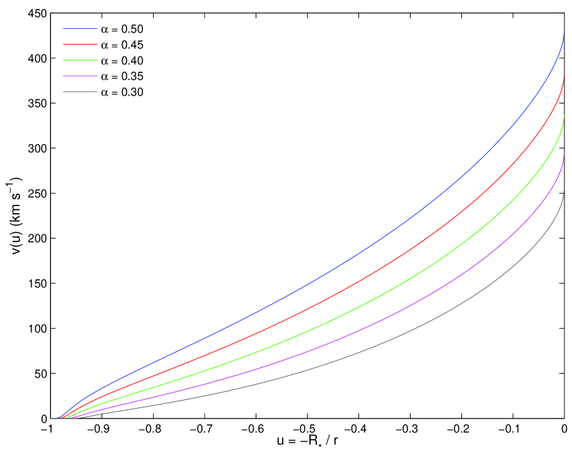
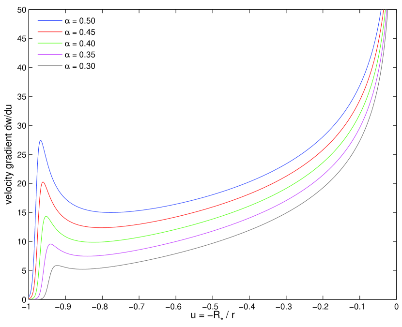
Figure 1: Left panel: velocity profiles as a function of the inverse radial coordinate $u$, for fixed $k$ = 0.3 and $\delta$ = 0.07 values, and various $\alpha$ values as indicated in the legend. Right panel: velocity gradients ($dw$/$du$) as a function of $u$ for the same solutions presented in the left panel.

Figure 1 illustrates the effect of lowering $\alpha$ from its starting value of 0.5 to 0.3, in steps of 0.05, on both the velocity structure (left panel) and its gradient (right panel) as a function of the inverse radial coordinate $u$. Clearly, lowering $\alpha$ corresponds to lower terminal velocities, but the overall, characteristic shape of the velocity profile is preserved for all values of $\alpha$ that we employed. Similarly, the velocity gradient shows less change in velocity (a smaller “hump”) occurring close to the stellar surface ($u=-1$) for lower $\alpha$ values, but retains its basic shape overall.

Table 2 is similar to Table 1, but with $\alpha$ and $\delta$ now held constant while $k$ is varied. Again, the first line in the table corresponds to the line-force parameters of Abbott (1982), and thus it is identical to the first line in Table 1. From these results, it is immediately clear that varying $k$ has only a marginal impact on the terminal velocity. Indeed, the only wind characteristic that $k$ significantly affects is the mass-loss rate, with greater $k$ values corresponding to greater mass-loss rates. Physically, a larger $k$ value represents a greater number of lines effectively contributing to the driving of the wind. When $k$ values greater than 9.0 were employed, no solutions could be found.

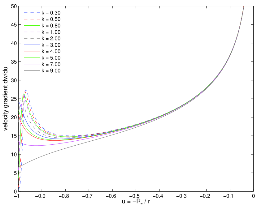
Figure 2: Left panel: velocity profiles as a function of the inverse radial coordinate $u$, for fixed $\alpha$ = 0.5 and $\delta$ = 0.07 values, and various $k$ values as indicated in the legend. Right panel: velocity gradients ($dw$/$du$) as a function of $u$ for the same solutions presented in the left panel. Note the change in the characteristic shape of the profile that occurs for $k$ values between 2.0 and 3.0.

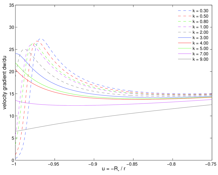
Figure 3: Magnified view of the behavior near the stellar surface of the velocity gradients shown in the right panel of Figure 2.

Figure 2 is similar to Figure 1, depicting the velocity structure and its gradient as a function of $u$ for the $k$ values listed in Table 2. As shown in the left panel of Figure 2, increasing the $k$ value results primarily in higher initial velocities at the stellar surface, but does not affect the terminal velocity or the characteristic behavior of the velocity profile overall. (However, we note that for $k\gtrsim 5.0$, the initial velocity is probably too high to be physical.) In contrast, the velocity gradient (shown in the right panel of Figure 2) completely loses its characteristic hump near the stellar surface somewhere between $2<k<3$. Figure 3 shows a magnified view of the velocity gradient near the stellar surface so that the transition to the new kind of behavior may be more clearly seen. The solutions corresponding to high $k$ values (i.e., $>2$ for this choice of $\alpha$ and $\delta$) and different velocity gradient structures (i.e., that do not display the characteristic hump) were previously unknown. To distinguish these high $k$, high $\Omega$ solutions from the other solutions, we refer to them as the $k\Omega$ solutions.

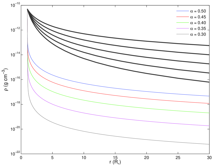
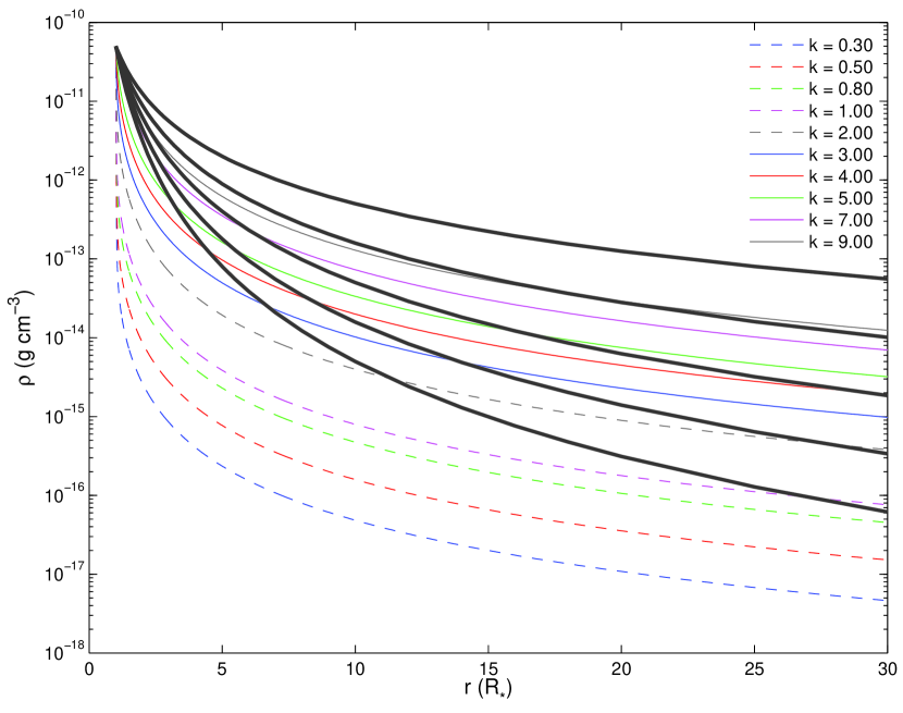
Figure 4: Comparison of equatorial density as a function of stellar radius for various Bedisk and Hydwind models. Left panel: $k=0.3$ and $\delta=0.07$ are held fixed while $\alpha$ varies from 0.5 to 0.3, in increments of 0.05, from top to bottom, shown in thin lines. Above this, ad hoc density distributions that follow a simple power-law drop-off, from $n=2.0$ to 4.0 from top to bottom, in increments of 0.5, are shown in thick lines. In both cases, the density at the stellar surface ($\rho_{*}=\rho_{0}$) is set to $5\times 10^{-11}$ g cm^-3. Right panel: $\alpha=0.5$ and $\delta=0.07$ are held fixed while $k$ takes the values 0.3, 0.5, 0.8, 1.0, 2.0, 3.0, 4.0, 5.0, 7.0, and 9.0, from bottom to top, shown in thin lines. Again, the same power-law governed equatorial densities shown in the left panel are shown in thick lines.

Tables 1 and  2 give some indication (when starting from the line force parameters of Abbott 1982) of which combinations of parameters yield mass-loss rates and terminal velocities similar to those predicted for Be stars. This information can be combined to generate the expected equatorial density structure that would result from the wind, which is something that can be directly compared to the ad hoc density structures typically assumed for Be stars. In Figure 4, the equatorial densities computed from the line-driven wind models are compared with ad hoc models of Be star disks. In both panels, typical ad hoc equatorial density profiles, governed by $n=2.0,2.5,3.0,3.5,$ and $4.0$ (from top to bottom) are shown in thick lines, while the equatorial density profiles computed from the hydrodynamic equations (with different values of the line force parameters) are shown in thin lines.

The left panel of Figure 4 depicts the solutions of constant $k=0.3$ and $\delta=0.07$, with $\alpha$ varying from 0.5 to 0.3 (in increments of 0.05) from top to bottom. Clearly, even the solution for the highest value of $\alpha$ has density values that are significantly lower than the density values that are typically assumed, and that have been shown to reproduce the observed H$\alpha$ emission signature. While lowering the value of $\alpha$ results in terminal velocities that better match those of Be stars, it obviously increases the discrepancy between the two density structures. Synthetic line profiles computed for these solutions only produce the stellar absorption profile, because, as expected, these densities are too low to produce any significant amount of emission.

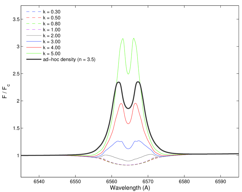
Figure 5: Synthetic H$\alpha$ profiles computed from the equatorial density structures obtained from the solution of the hydrodynamic equations and used as input into the radiative transfer code Bedisk, shown in thin lines, for $k$ values of 0.3, 0.5, 0.8, 1.0, 2.0, 3.0, 4.0, and 5.0. For comparison, an emission profile computed from the ad hoc density structure $\rho=5\times 10^{-11}$ g cm${}^{-3}(r/R_{*})^{-3.5}$ is also shown. An inclination of $i=35\arcdeg$ was assumed for all profiles. Clearly, $k\leq 1$ produces only an absorption profile, but emission begins for $k>1.0$ and becomes progressively stronger for higher $k$ values.

The right panel of Figure 4 depicts the solutions of constant $\alpha=0.5$ and $\delta=0.07$, with $k$ increasing from 0.3, to 0.5, 0.8, 1.0, 2.0, 3.0, 4.0, 5.0, 7.0, and 9.0, from bottom to top. What is seen in this plot is that for $k$ values $\sim 2$ and greater, the equatorial densities computed by the two different methods become comparable. Using these equatorial densities as input into Bedisk, significant emission was found for $k\geq 2$. This is depicted in Figure 5, which shows the emission profiles for $k$ = 0.3, 0.5, 0.8, 1.0, 2.0, 3.0, 4.0, and 5.0 in thin lines. The lowest $k$ values ($k\leq 1$) produce only the stellar absorption profile, with the emission first becoming appreciable at $k=2$ and increasing in strength with increasing $k$. For comparison, a synthetic line profile created from an ad hoc equatorial density structure with $\rho_{0}=5\times 10^{-11}$ g cm^-3 and $n=3.5$ (the value of $n$ most commonly found for Be stars) is shown in the thick line.

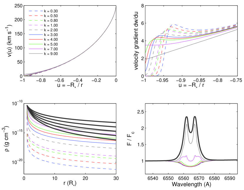
Figure 6: Results for simulations performed using a fixed $\alpha$ value of 0.3, $\delta$ = 0.07, and various $k$ values as given in the legend in the top left panel. The legend applies to all plots in the figure. In the lower left panel, the thick, dark gray lines correspond to the same ad hoc density structures shown in Figure 4, and in the lower right panel, the thick, dark line corresponds to the same emission profile from an ad hoc density structure that is shown in Figure 5.

From the above investigation, we deduce that the lowest value of $\alpha$ used in this study ($\alpha=0.3$) may better describe Be star disks because of its low outflow velocity; thus, we have further explored this parameter space. In Table 3, we show the mass-loss rates and terminal velocities for solutions with $\alpha=0.3$ and $\delta=0.07$ held fixed while $k$ is again allowed to vary. In Figure 6, we show the characteristics of these solutions. The velocities (shown in the top left panel of Figure 6) of these low-$\alpha$ solutions are remarkably constant over the whole range of $k$ values that we employed. We note that, even at high $k$ values, the solutions do not obtain high velocities at the stellar surface (i.e., they do not become unphysical), which represents a marked contrast to the solutions obtained with $\alpha$ fixed at 0.5. In the top right panel of this same figure, we show the velocity gradients of the $\alpha$ = 0.3 solutions in the region close to the stellar surface. Solutions of the new $k\Omega$-type are found for $k=7.0$ and $k=9.0$. In the bottom left panel, the densities of the $\alpha=0.3$ solutions are compared with typical ad hoc equatorial densities corresponding to $n=2.0$ (topmost dark gray line) to $n=4.0$ (bottom-most dark gray line) and changing by increments of 0.5 (similarly to Figure 4.) Finally, in the bottom right panel, the emission expected from these equatorial densities is shown. In the $\alpha=0.3$ case, we see significant emission only occurring from $k=7.0$ and higher. This corresponds to the same value of $k$ that marks the emergence of the $k\Omega$ solutions.

4 Summary and Discussion

Previous attempts to model Be stars in the context of radiatively driven winds added a centrifugal force term to the momentum equation, to account for the effect of rapid rotation, but still drew solutions from the family of solutions originally obtained by Castor et al. (1975) in their pioneering work. Indeed, Castor et al. (1975), who had neglected rotation entirely in their model, had shown the existence of only one family of physical solutions. Curé & Rial (2007) confirmed that the standard m-CAK singular point is the only one that satisfies the boundary condition at the stellar surface when rotation is neglected. All such solutions, however, have terminal velocities that are too high to be compatible with those found in Be star disks.

When Curé (2004) performed a reanalysis of the hydrodynamic equations with a momentum equation that included the centrifugal force term, he found a new family of solutions (the $\Omega$-slow solutions) with much lower terminal velocities and higher mass-loss rates. He showed that while these new solutions are in fact present for all rotation rates, the traditional CAK solutions actually cease to exist for $v_{\rm{rot}}/v_{\rm{crit}}\approx 0.75$, and therefore these new solutions are the only ones that can exist for very high rotation rates. The existence of a slowly outflowing, dense wind for $v_{\rm{rot}}\geq 0.75v_{\rm{crit}}$ seemed immediately appropriate for a Be star, and we therefore felt it merited further investigation.

We started our investigation from the line-force parameters for a B1V star ($T_{\rm{eff}}=25\,000$ K) as given by Abbott (1982): $k$ = 0.3, $\alpha$ = 0.5, and $\delta$ = 0.07. These parameters yield a terminal velocity that is slightly too high for Be stars (by about a factor of two), and a mass-loss rate that is insufficient to build up an equatorial density structure that produces significant emission. We recall, however, that the parameters derived by Abbott are done so under the assumptions of the original CAK theory, and may no longer be appropriate for the new family of $\Omega$-slow solutions. Thus, we systemically varied $\alpha$ and $k$ to see what values of these two parameters produce terminal velocities and mass-loss rates that agree with the values found for Be stars. We have shown that if $k$ and $\delta$ are fixed at 0.3 and 0.07, respectively, then $\alpha$ = 0.3 produces $v_{\infty}=256$ km s^-1. This is in good agreement with Poeckert & Marlborough (1978), who suggested that the outflow velocity of a Be star disk was of the order of $\sim$200 km s^-1. Alternately, if $\alpha$ and $\delta$ are held fixed at 0.5 and 0.07, respectively, $k$ values of 2.0 and greater produce equatorial densities comparable to the ones assumed in the ad hoc scenario, and also produce appreciable emission if those equatorial density structures are used as input in Bedisk.

Finally, because solutions with $\alpha=0.3$ had the best agreement with the terminal velocity predicted for Be stars, we further explored this parameter space. By allowing $k$ to vary over the same range as in our previous experiment, we found that all solutions with $\alpha=0.3$ retained low velocities near the stellar surface (meaning that high $k$ values did not lead to unphysical solutions in this case). By examining the velocity gradient of these solutions, it was found that the $k\Omega$ solutions emerged around $k\gtrsim 7.0$, which is considerably higher than when $\alpha=0.5$ ($k\Omega$ solutions emerge at $k\gtrsim 2$). Furthermore, only solutions with $k=7.0$ or higher produced significant emission in our simulations. However, as outlined in the Future Work section (see below), we feel there are additional alterations and refinements that we could apply to our model that may allow us to achieve larger equatorial densities from smaller $k$ values.

One aspect of our calculation that merits additional discussion is that, because Bedisk considers the disk to be in Keplerian rotation, and considers this to be the only source of profile broadening, outflow in the disk is neglected. However, the bulk of the H$\alpha$ emission has been shown to arise from the region $\sim 5-15R_{*}$ from the stellar surface, and as shown in Table 3 of Poeckert & Marlborough (1978), the outflow velocities at $r/R_{*}$ = 6.0 and $r/R_{*}$ = 18.0 are predicted to be 25 km s^-1 and 125 km s^-1, respectively. Therefore, especially for the innermost region of H$\alpha$ emission, where densities are highest (and thus the majority of the emission is produced), the outflow velocity is negligible compared with the rotational velocity.

In performing the systematic investigation of the line-force parameters, we discovered a new behavior in the velocity gradient for solutions with high $k$ values, which we call the $k\Omega$ solutions. This new behavior was observed to emerge between $2\leq k\leq 3$, when $\alpha$ and $\delta$ are 0.5 and 0.07, respectively. While $k$ has traditionally been found to have a value of $\sim 0.5$ for a star with the effective temperature we have adopted in our model, we recall that all of the previous analyses have been performed in the regime of the fast winds that pass through the original m-CAK critical point. In a private communication with Joachim Puls (2014), he stated that, generally, $k\sim 1/\alpha$; since we employ values of $\alpha=0.5$ to $0.3$, $k=2$ or $k\gtrsim 3$ are predicted from this relation. When $\alpha$ = 0.5 and $k\geq 5$, however, we find that the solutions become unphysical due to the high initial velocities that they exhibit.

5 Future Work

We have begun our investigation into the possible role of the $\Omega$-slow solutions in the formation of Be star disks by first examining the equatorial density structure that arises from such winds, i.e., we have examined the 1D solutions. We have compared these equatorial density structures to the ad hoc scenario in which a given initial density is assumed to fall off according to a single power law with increasing radial distance from the star. In order to estimate the magnitude of the H${\alpha}~{}$emission that might arise from $\Omega$-slow solutions, various equatorial density structures computed from these solutions were used as input into the code Bedisk. We have shown that significant H$\alpha$ emission can be produced by some combinations of the line-force parameters.

In a future paper, we plan to do a comparison of the full 2D structure computed from the hydrodynamic equations versus the 2D structure computed by Bedisk. If the vertical structure computed by Hydwind has more material in the regions close to the equatorial plane (i.e., slightly above and below it), then it may be possible to produce significant emission in models with lower $k$ values than the ones used here.

An additional important consideration may be the inclusion of the oblate finite disk correction factor. For simplicity, we have started from the usual finite disk correction factor, which approximates the star as a uniformly bright sphere. Realistically, however, when a star is rotating close to its critical velocity (such as in the case of Be stars), the star becomes an oblate spheroid, with a cooler equatorial region and hotter poles. As shown in Araya et al. (2011), the use of an oblate finite disk correction factor results in higher mass loss rates in the equatorial plane. Thus, this may represent yet another way to reproduce emission profiles with smaller $k$ values than we have employed in this work.

Table 1: B1V Wind Models with $k=0.3$, $\delta=0.07$, and Varying $\alpha$ Values.

$\alpha$	$\dot{M}$	$v_{\infty}$
	(10${}^{-6}M_{\sun}\,yr^{-1}$)	(km s-1)
0.50	4.273$\times 10^{-3}$	430
0.45	9.632$\times 10^{-4}$	381
0.40	1.428$\times 10^{-4}$	337
0.35	1.116$\times 10^{-5}$	295
0.30	3.038$\times 10^{-7}$	256

Note. — All models assume an initial density $\rho_{*}=5\times 10^{-11}$ g cm^-3.

Table 2: B1V Wind Models with $\alpha=0.5$, $\delta=0.07$, and Varying $k$ Values.

$k$	$\dot{M}$	$v_{\infty}$
	(10${}^{-6}M_{\sun}\,yr^{-1}$)	(km s-1)
0.30	4.273$\times 10^{-3}$	430
0.50	1.402$\times 10^{-2}$	430
0.80	4.182$\times 10^{-2}$	430
1.00	7.026$\times 10^{-2}$	430
2.00	3.522$\times 10^{-1}$	430
3.00	9.042$\times 10^{-1}$	430
4.00	1.765$\times 10^{0}$	430
5.00	2.966$\times 10^{0}$	430
7.00	6.482$\times 10^{0}$	432
9.00	1.161$\times 10^{1}$	435

Note. — All models assume an initial density $\rho_{*}=5\times 10^{-11}$ g cm^-3.

Table 3: B1V Wind Models with $\alpha=0.3$, $\delta=0.07$, and Varying $k$ Values.

$k$	$\dot{M}$	$v_{\infty}$
	(10${}^{-6}M_{\sun}\,yr^{-1}$)	(km s-1)
0.30	3.038$\times 10^{-7}$	256
0.50	2.800$\times 10^{-6}$	256
0.80	2.160$\times 10^{-5}$	256
1.00	5.700$\times 10^{-5}$	256
2.00	1.161$\times 10^{-3}$	256
3.00	6.765$\times 10^{-3}$	256
4.00	2.363$\times 10^{-2}$	256
5.00	6.235$\times 10^{-2}$	256
7.00	2.692$\times 10^{-1}$	256
9.00	8.028$\times 10^{-1}$	256

Note. — All models assume an initial density $\rho_{*}=5\times 10^{-11}$ g cm^-3.

References

- Abbott (1982) Abbott, D. C. 1982, ApJ, 259, 282
- Araya et al. (2011) Araya, I., Curé, M., Granada, A., & Cidale, L. S. 2011, in IAU Symp. 272, ed. C. Neiner, G. Wade, G. Meynet, & G. Peters, (Cambridge: Cambridge Univ. Press), 83
- Baade (1982) Baade, D. 1982, A&A, 105, 65
- Bjorkman & Cassinelli (1993) Bjorkman, J. E., & Cassinelli, J. P. 1993, ApJ, 409, 429
- Castor et al. (1975) Castor, J. I., Abbott, D. C., & Klein, R. I. 1975, ApJ, 195, 157
- Cote & Waters (1987) Cote, J., & Waters, L. B. F. M. 1987, A&A, 176, 93
- Curé (2004) Curé, M. 2004, ApJ, 614, 929
- Curé & Rial (2007) Curé, M., & Rial, D. F. 2007, Astronomische Nachrichten, 328, 513
- de Araujo & de Freitas Pacheco (1989) de Araujo, F. X., & de Freitas Pacheco, J. A. 1989, MNRAS, 241, 543
- Friend & Abbott (1986) Friend, D. B., & Abbott, D. C. 1986, ApJ, 311, 701
- Jones et al. (2008) Jones, C. E., Tycner, C., Sigut, T. A. A., Benson, J. A., & Hutter, D. J. 2008, ApJ, 687, 598
- Marlborough & Zamir (1984) Marlborough, J. M., & Zamir, M. 1984, ApJ, 276, 706
- Okazaki (1991) Okazaki, A. T. 1991, PASJ, 43, 75
- Okazaki (1996) —. 1996, PASJ, 48, 305
- Owocki et al. (1996) Owocki, S. P., Cranmer, S. R., & Gayley, K. G. 1996, ApJ, 472, L115
- Pauldrach et al. (1986) Pauldrach, A., Puls, J., & Kudritzki, R. P. 1986, A&A, 164, 86
- Poe & Friend (1986) Poe, C. H., & Friend, D. B. 1986, ApJ, 311, 317
- Poeckert & Marlborough (1978) Poeckert, R., & Marlborough, J. M. 1978, ApJ, 220, 940
- Porter (1996) Porter, J. M. 1996, MNRAS, 280, L31
- Sigut & Jones (2007) Sigut, T. A. A., & Jones, C. E. 2007, ApJ, 668, 481
- Silaj et al. (2010) Silaj, J., Jones, C. E., Tycner, C., Sigut, T. A. A., & Smith, A. D. 2010, ApJS, 187, 228
- Stee & de Araujo (1994) Stee, P., & de Araujo, F. X. 1994, A&A, 292, 221
- Townsend et al. (2004) Townsend, R. H. D., Owocki, S. P., & Howarth, I. D. 2004, MNRAS, 350, 189
- Underhill et al. (1982) Underhill, A. B., Doazan, V., Lesh, J. R., Aizenman, M. L., & Thomas, R. N. 1982, in B Stars With and Without Emission Lines, (NASA SP-456), 140
- Waters (1986) Waters, L. B. F. M. 1986, A&A, 162, 121
- Waters et al. (1987) Waters, L. B. F. M., Cote, J., & Lamers, H. J. G. L. M. 1987, A&A, 185, 206