One-dependent coloring by finitary factors

Abstract.

Holroyd and Liggett recently proved the existence of a stationary $1$-dependent $4$-coloring of the integers, the first stationary $k$-dependent $q$-coloring for any $k$ and $q$. That proof specifies a consistent family of finite-dimensional distributions, but does not yield a probabilistic construction on the whole integer line. Here we prove that the process can be expressed as a finitary factor of an i.i.d. process. The factor is described explicitly, and its coding radius obeys power-law tail bounds.

1. Introduction

Let $X=(X_{i})_{i\in\mathbb{Z}}$ be a stochastic process, i.e. a random element of $\mathbb{R}^{\mathbb{Z}}$. We call $X$ a (proper) $q$-coloring if each $X_{i}$ takes values in $[q]:=\{1,\ldots,q\}$, and almost surely we have $X_{i}\neq X_{i+1}$ for all $i\in\mathbb{Z}$. A process $X$ is called $k$-dependent if the random vectors $(X_{i})_{i\in A}$ and $(X_{i})_{i\in B}$ are independent of each other whenever $A$ and $B$ are two subsets of $\mathbb{Z}$ satisfying $|a-b|>k$ for all $a\in A$ and $b\in B$. A process is finitely dependent if it is $k$-dependent for some integer $k$. A process $X$ is stationary if $(X_{i})_{i\in\mathbb{Z}}$ and $(X_{i+1})_{i\in\mathbb{Z}}$ are equal in law. Holroyd and Liggett [4] proved the existence of a stationary $1$-dependent $4$-coloring, and a stationary $2$-dependent $3$-coloring. These were the first known stationary finitely dependent colorings. The descriptions of the processes given in [4] are mysterious, and involve specifying a consistent family of finite-dimensional distributions rather than an explicit construction on $\mathbb{Z}$.

A process $X$ is a factor of a process $Y=(Y_{i})_{i\in\mathbb{Z}}$ if it is equal in law to $F(Y)$, where the function $F$ is translation-equivariant, i.e. it commutes with the action of translations of $\mathbb{Z}$. A factor of a stationary process is necessarily stationary. The factor is finitary if for almost every $y$ (with respect to the law of $Y$) there exists $t<\infty$ such that whenever $y^{\prime}$ agrees with $y$ on the interval $\{-t,\ldots,t\}$, the resulting values assigned to $0$ agree, i.e. $F(y^{\prime})_{0}=F(y)_{0}$. In that case we write $T(y)$ for the minimum such $t$, and we call the random variable $T=T(Y)$ the coding radius of the factor. In other words, in a finitary factor, the symbol $X_{0}$ at the origin can be determined by examining only those variables $Y_{i}$ within a random, finite, but perhaps unbounded distance $T$ from the origin.

Our main result is that finitely dependent coloring can be done by a finitary factor.

Theorem 1.

There exists a $1$-dependent $4$-coloring of $\mathbb{Z}$ that is a finitary factor of an i.i.d. process. The coding radius $T$ satisfies

$$\mathbb{P}(T>t)<c\,t^{-\alpha},\qquad t\geq 1,$$

for some absolute constants $c,\alpha>0$.

Our proof of Theorem 1 gives an explicit description of the finitary factor $F$, and our $4$-coloring $X$ is actually the same as the one in [4] (but constructed in a different way). The power $\alpha$ that we obtain is strictly less than $1$ (in fact, it is rather close to $0$), and $T$ has infinite mean. We do not know whether there exists a finitely dependent coloring that is a finitary factor of an i.i.d. process with finite mean coding radius.

The result of [4] that stationary finitely dependent colorings exist is surprising for several reasons. A block factor is a finitary factor with bounded coding radius (so that $X_{i}$ is a fixed function of $Y_{j-t},\ldots,Y_{j+t}$). Block factors of i.i.d. processes provide a natural means to construct finitely dependent processes: if the coding radius is at most $k$ then the process is $2k$-dependent. Indeed, for some time it was an open problem whether every finitely dependent process was a block factor of an i.i.d. process (see e.g. [7]). The first published counterexample appears in [1]. Prior to [4], there was a (very reasonable) belief that most “natural” finitely dependent processes are block factors (see e.g. [2]). However, it turns out that no block-factor coloring exists (see e.g. [9, 6, 4]). Hence, the result of [4] shows that on the contrary, the very natural task of coloring serves to distinguish between block factors and finitely dependent processes. See [4] for more on the history of this problem.

Extensions and applications

We next discuss other $k$ and $q$. One can attempt to apply our method to the $2$-dependent $3$-coloring of [4], but we will see that it encounters a fundamental obstacle in this case. By a result of Schramm (see [6] or [4]), no stationary $1$-dependent $3$-coloring exists. The stationary $1$-dependent $4$-coloring is conjectured in [4] to be unique. (And $(k,q)=(1,4)$ is shown to be a critical point in a certain sense). It is plausible that the $2$-dependent $3$-coloring is unique also, although the evidence is less strong in this case. It is natural to expect that there is far more flexibility in $k$-dependent $q$-colorings for larger $k$ and $q$, although constructing examples seems difficult, and currently very few are known. In [5], a $1$-dependent $q$-coloring that is symmetric in the colors is constructed for each $q\geq 4$. Besides these colorings and the two in [4], and straightforward embellishments thereof, no other examples are known. One such embellishment, described in [4], is a $3$-dependent $3$-coloring that arises as a simple block factor of the $1$-dependent $4$-coloring. Since a composition of finitary factors is finitary, Theorem 1 implies that this $3$-dependent $3$-coloring is a finitary factor of an i.i.d. process also.

In light of the above observations, a natural conjecture is that there exists a $k$-dependent $q$-coloring that is a finitary factor of an i.i.d. process with finite mean coding radius if and only if $k\geq 1$, $q\geq 3$, and $(k,q)\not\in\{(1,3),(2,3),(1,4)\}$.

Coloring on $\mathbb{Z}$ is a key case within a more general framework. It is proved in [4] that for every shift of finite type $S$ on $\mathbb{Z}$ that satisfies a certain non-degeneracy condition, there is a stationary finitely dependent process that lies a.s. in $S$. Additionally, in the $d$-dimensional lattice $\mathbb{Z}^{d}$, there exist a $1$-dependent $q$-coloring and a $k$-dependent $4$-coloring (where $q$ and $k$ depend on $d$). These facts are proved by starting from the $1$-dependent $4$-coloring of $\mathbb{Z}$ and applying block-factors (in some cases using methods developed in [6]). Consequently, using our Theorem 1, each of these processes is a finitary factor of an i.i.d. process.

The question of $q$-coloring as a finitary factor of a i.i.d. process (without the finite dependence requirement) is addressed in [6], including on $\mathbb{Z}^{d}$. Depending on $q$ and $d$, the best coding radius tail that can be achieved is either a power law (when $q=3$ and $d\geq 2$) or a tower function (when $q\geq 4$ and $d\geq 2$, or $q\geq 3$ and $d=1$).

Coloring has applications in computer science. For instance, colors may represent time schedules or communication frequencies for machines in a network, and adjacent machines are not permitted to conflict with each other. Finite dependence implies a security benefit — an adversary who gains knowledge of some colors learns nothing about the others, except within a fixed finite distance. A finitary factor of an i.i.d. process is also desirable. It has the interpretation that the colors can be computed by the machines in distributed fashion, based on randomness generated locally, combined with communication with machines within a finite distance. All machines follow the same protocol, and no central authority is needed. See e.g. [8, 9] for more information. Unfortunately, the finitary factor of Theorem 1 is of limited practical use because of the heavy tail of $T$ — the communication distance to determine the color at the origin is almost surely finite, but typically huge.

Outline of Proof

As mentioned earlier, the construction in [4] involves specifying the law of the coloring restricted to a finite interval, and proving that these laws form a consistent family. The law on an interval has a probabilistic interpretation, involving inserting colors in a random order. However, this order is not uniform, but weighted to favor insertions at the endpoints. The random orders themselves are therefore not consistent between different intervals. Using uniformly random orders instead gives consistent orders but inconsistent colorings. However, we show that, in the limit of a long interval, the choice of weight does not affect the law near the center. The key observation is that endpoint insertions are typically few (in fact $\Theta(\log n)$ in an interval of length $n$), even under the weighting, so their effect can be neglected.

To obtain a factor of an i.i.d. process we introduce a “graphical representation” of the insertion process that extends naturally to $\mathbb{Z}$. Each inserted color must itself be randomly chosen, and must differ from its neighbors. With $4$ (or more) colors, this means that there is a choice, and we use this to define special locations at which the random color can be decoupled from its surroundings, leading to a finite coding radius.

2. The construction

Fix a number of colors $q\geq 3$. Let $(U_{i})_{i\in\mathbb{Z}}$ be i.i.d. random variables, with each $U_{i}$ uniformly distributed on the interval $[0,1]$. We interpret $U_{i}$ as the arrival time of the integer $i$. The idea is that when an integer arrives, it chooses a color uniformly at random from the colors that are not present among its two current neighbors (i.e. the nearest integers to the left and to the right that arrived before it). Thus, for $i\in\mathbb{Z}$, define:

$$L(i) :=\max\{j<i:U_{j}<U_{i}\};$$

$$R(i) :=\min\{j>i:U_{j}<U_{i}\}.$$

Let $(\phi_{i})_{i\in\mathbb{Z}}$ be i.i.d. permutations, with each $\phi_{i}$ uniformly distributed on the symmetric group $S_{q}$ of permutations of $[q]$, and with $(\phi_{i})_{i\in\mathbb{Z}}$ independent of $(U_{i})_{i\in\mathbb{Z}}$. The idea is that $\phi_{i}$ denotes the preference order of integer $i$ over the $q$ colors, with $\phi_{i}(j)$ being $i$’s $j$th favorite color, for $j=1,\ldots,q$.

Given $(U_{i})_{i\in\mathbb{Z}}$ and $(\phi_{i})_{i\in\mathbb{Z}}$, we seek a sequence $(X_{i})_{i\in\mathbb{Z}}\in[q]^{\mathbb{Z}}$ that satisfies the system of equations

(1) $$\begin{split}X_{i}&=\phi_{i}(K),\qquad i\in\mathbb{Z},\\ \text{where}\quad K&=K(i)=\min\Bigl{\{}k\in[q]:X_{L(i)}\neq\phi_{i}(k)\neq X_{R(i)}\Bigr{\}}.\end{split}$$

Thus, the integer $i$ is assigned its favorite color $X_{i}$ among those that have not been taken by its current neighbors at its arrival time.

It is clear that any solution $(X_{i})_{i\in\mathbb{Z}}$ to (1) is a $q$-coloring: we have $X_{L(i)}\neq X_{i}\neq X_{R(i)}$, but if $U_{i+1}<U_{i}$ then $R(i)=i+1$, and otherwise $L(i+1)=i$. However, it is not immediately clear whether there is a solution: $X_{i}$ is expressed in terms of $X_{L(i)}$ and $X_{R(i)}$, so the computation apparently involves an infinite regress.

The outcome depends crucially on the number of colors. By a similar argument to the above, any solution must have $X_{L(i)}\neq X_{R(i)}$ for all $i$, so precisely two colors are ruled out for $X_{i}$ by the requirement $X_{L(i)}\neq X_{i}\neq X_{R(i)}$. Therefore, if $q=3$ then only one color remains, so the preference order $\phi_{i}$ is irrelevant. On the other hand, if $q\geq 4$ then $i$ has a choice, therefore it will never need its $4$th favorite color $\phi_{i}(4)$ or worse. This will allow us to end the regress: if the favorite of $i$ is the $4$th favorite of $L(i)$ and $R(i)$, then we know that $i$ will receive its favorite color. Using this idea, we will prove the following in the next section.

Proposition 2.

Fix $q\geq 4$. Let $(U_{i})_{i\in\mathbb{Z}}$ be i.i.d. uniform on $[0,1]$, and $(\phi_{i})_{i\in\mathbb{Z}}$ i.i.d. uniform on $S_{q}$, independent of each other. Almost surely, the system of equations (1) has a unique solution $(X_{i})_{i\in\mathbb{Z}}$. Moreover, $(X_{i})_{i\in\mathbb{Z}}$ is a finitary factor of the i.i.d. process $((U_{i},\phi_{i}))_{i\in\mathbb{Z}}$, with coding radius $T$ satisfying

$$\mathbb{P}(T>t)<c\,t^{-\alpha},\qquad t>0,$$

for some $c,\alpha>0$ depending only on $q$.

In the later sections we will prove that when $q=4$, the process $(X_{i})_{i\in\mathbb{Z}}$ coincides with the $1$-dependent $4$-coloring constructed in [4].

When $q=3$ it is not difficult to check that a.s. the system of equations (1) has exactly $3!=6$ solutions. There is a.s. a uniquely defined partition of $\mathbb{Z}$ into $3$ sets, which depends on $(U_{i})_{i\in Z}$ but not on $(\phi_{i})_{i\in\mathbb{Z}}$, and each solution corresponds to an assignment of colors to the $3$ sets. If this assignment chosen to be a uniformly random permutation in $S_{3}$, independent of $(U_{i})_{i\in Z}$, then the resulting process is the $2$-dependent $3$-coloring of [4]. However, this “global assignment” step means that the construction is not a finitary factor.

3. Coding radius bound

In this section we prove Proposition 2. Motivated by the discussion of the previous section, given $(U_{i},\phi_{i})_{i\in\mathbb{Z}}$, we say that the integer $i$ is lucky if

$$\phi_{L(i)}(4)=\phi_{i}(1)=\phi_{R(i)}(4).$$

(We could allow $\phi_{L(i)}(k),\phi_{R(i)}(k^{\prime})$ for any $k,k^{\prime}\geq 4$ here, but the above definition suffices, and in any case our main focus is $q=4$). Here is the key step.

Lemma 3.

Let $q\geq 4$ and let $(U_{i},\phi_{i})_{i\in\mathbb{Z}}$ be as in Proposition 2. For any $m\geq 0$, a.s. there exist lucky integers $A$ and $B$ with $[-m,m]\subseteq[A,B]$ such that

(2) $$\max\{U_{A},U_{B}\}<\min\{U_{i}:i\in(A,B)\}.$$

Moreover, $A$ and $B$ can be chosen so that

(3) $$\mathbb{P}\Bigl{(}\max\bigl{\{}|L(A)|,|R(A)|,|L(B)|,|R(B)|\bigr{\}}>t\Bigr{)}<c\,t^{-\alpha},\quad t\geq 1,$$

for some positive constants $c=c(q,m)$ and $\alpha=\alpha(q)>0$.

Proof of Proposition 2.

Using Lemma 3 with $m=0$, let $T\geq 1$ be the smallest integer for which there exist lucky $A\leq 0\leq B$ satisfying (2) for which the maximum appearing in (3) is at most $T$. This $T$ can be determined from the variables $(U_{i},\phi_{i})$ for $|i|\leq T$ (by examining the integers $i$ in order of absolute value), and Lemma 3 states that it satisfies the sought tail bound.

Since $A$ and $B$ are lucky, in any solution to (1) we have that $X_{A}=\phi_{A}(1)$ and $X_{B}=\phi_{B}(1)$. Condition (2) implies that for all $i\in(A,B)$ we have $L(i),R(i)\in[A,B]$. Therefore, the remaining colors $(X_{i})_{i\in(A,B)}$ in the interval can be determined via (1) from $((U_{i},\phi_{i}))_{i\in[A,B]}$, by considering them in increasing order of $U_{i}$. In particular, we can determine $X_{0}$.

By stationarity, we can similarly find an interval $[A_{i},B_{i}]\ni i$ corresponding to any $i\in\mathbb{Z}$. By applying Lemma 3 with larger $m$, it is easy to see that the colors $(X_{j})_{j\in[A_{i},B_{i}]}$ computed from different intervals are consistent with each other and with (1). We conclude that the resulting $(X_{i})_{i\in\mathbb{Z}}$ is the unique solution to (1), and is a finitary factor of $(U_{i},\phi_{i})_{i\in\mathbb{Z}}$ with coding radius $T$. ∎

Before proving Lemma 3, we briefly discuss where the power law tail bound comes from. First note that even $R(0)$ has mean $\infty$, since it is the location of the second record minimum of the i.i.d. sequence $(U_{i})_{i\geq 0}$ (the first record being at $i=0$). However, the integer $B$ of Lemma 3 is much larger than this. In addition to being a record, it must be lucky. Consider the simplified situation in which $(G_{i})_{i\in\mathbb{Z}}$ are independent events of probability $p$, independent of $(U_{i})_{i\in\mathbb{Z}}$. Let $J$ be the smallest positive integer for which $G_{J}$ occurs and $(U_{i})_{i\geq 0}$ has a record minimum at $J$. Then, by the standard fact (see e.g. [3, Example 2.3.2]) that there is a record at $i$ with probability $1/i$, independently for different $i$, we have

$$\mathbb{P}(J>t)=\prod_{i=1}^{t}\Bigl{(}1-\frac{p}{i}\Bigr{)}=\Theta(t^{-p})\quad\text{as }t\to\infty.$$

For $q=4$, the probability that an integer is lucky is $1/16$, therefore at best we can expect a power $\alpha=1/16$ in our tail bound on the coding radius. We have not attempted to optimize $\alpha$, so the bound we prove is in fact much smaller than this. At the expense of additional complexity, our method below could be adapted to prove a power closer to $1/16$. By refining the definition of lucky integers to encompass more complicated local patterns of preferences, the bound could likely be increased beyond $1/16$. However, any such improvement would still result in a power $\alpha$ strictly less than $1$, and infinite mean coding radius.

Proof of Lemma 3.

To find suitable $A$ and $B$ we examine the integers in order of absolute value. Call $i\in\mathbb{Z}$ an absolute record if $U_{i}$ is smaller than all the terms that precede it in the sequence $U_{i_{1}},U_{i_{2}},U_{i_{3}},\ldots,$ where $(i_{1},i_{2},i_{3},\ldots)=(0,1,-1,2,-2,\ldots)$ Since the reordered sequence is of course still i.i.d., $i_{j}$ is an absolute record with probability $1/j$, and the events that different integers are absolute records are independent.

Now, for $n\geq 1$, we compute the probability

$$\begin{split}\begin{aligned} \mathbb{P}\Bigl{[}&[2^{n},2^{n+1})\text{ contains exactly one absolute record, and}\\ &(-2^{n+1},-2^{n}]\text{ contains no absolute records}\Bigr{]}\end{aligned}\\ \begin{aligned} &=\prod_{j=2^{n}}^{2^{n+1}-1}\Bigl{(}1-\frac{1}{2j}\Bigr{)}\Bigl{(}1-\frac{1}{2j+1}\Bigr{)}\cdot\sum_{i=2^{n}}^{2^{n+1}-1}\frac{\tfrac{1}{2i}}{1-\tfrac{1}{2i}}\\ &\geq\frac{1}{8}\end{aligned}\end{split}$$

(The product telescopes, and the sum can be bounded via its smallest term). Similarly, the probability that $(-2^{n+1},-2^{n}]$ contains exactly one absolute record while $[2^{n},2^{n+1})$ contains none is also at least $1/8$.

For $n\geq 1$, let $E_{n}$ be the event that there exist integers $a,b,c,d,e$ satisfying all of:

• $2^{5n}{\leq a<}2^{5n+1}{\leq b<}2^{5n+2}{\leq-c<}2^{5n+3}{\leq-d<}2^{5n+4}{\leq e<}2^{5n+5}$;

• $a,b,c,d,e$ are the only absolute records in

  $(-2^{5n+5},-2^{5n}]\cup[2^{5n},2^{5n+5})$;

• $\phi_{c}(4)=\phi_{a}(1)=\phi_{b}(4)$, and $\phi_{d}(4)=\phi_{c}(1)=\phi_{e}(4)$.

On $E_{n}$, we have $L(a)=c$, $R(a)=b$, $L(c)=d$, and $R(c)=e$; therefore, $a$ and $c$ are lucky; we take $A=c$ and $B=a$. We have $[-2^{5n},2^{5n}]\subseteq[A,B]$, and (2) holds. Moreover, the maximum in (3) is at most $2^{5n+5}$.

On the other hand, the events $(E_{n})_{n\geq 1}$ are independent. Using the previous computation, we have $\mathbb{P}(E_{n})\geq(1/8)^{5}(1/q)^{4}$. We conclude that the claimed bound holds with $\alpha=-\log(1-8^{-5}q^{-4})/(5\log 2)$. (When $q=4$, this is approximately $3\times 10^{-8}$). ∎

4. Weighted insertion processes

We introduce a family of random proper colorings of finite intervals, which we call weighted insertion (WI) colorings. Throughout this section, an interval $[a,b]$ is understood to denote the set of integers $[a,b]\cap\mathbb{Z}$, where $a,b\in\mathbb{Z}$. A finite sequence $x=(x_{i})_{i\in[a,b]}$ is a coloring of $[a,b]$ if $x_{i}\neq x_{i+1}$ for all $a\leq i<b$.

Fix a number of colors $q\geq 3$ and a real weight $w>0$. For $n\geq 1$, we define the WI coloring $X=X^{[n]}\in[q]^{n}$ of the interval $[n]=[1,n]$ (with parameters $(w,q)$), via an iterative constriction. When $n=1$, $X^{[1]}$ is a sequence of length $1$ consisting of a uniformly random color from $[q]$. Conditional on $X^{[n]}=(X_{1},\ldots,X_{n})$, we construct $X^{[n+1]}$ by the following insertion procedure.

First, we choose a random insertion point $I$, with law that is uniform on $[1,n+1]$ except that the two endpoints have bias $w$:

$$\mathbb{P}(I=i)=\begin{cases}\frac{w}{2w+n-1},&i=1\text{ or }n+1;\\ \frac{1}{2w+n-1},&i=2,\ldots,n.\end{cases}$$

Then we choose a random color $Z$ uniformly from the set

$$[q]\setminus\{X_{I-1},X_{I}\}$$

of colors that differ from the neighbors of the insertion point. Here, $X_{0}$ and $X_{n+1}$ are taken to be $\infty$ (say), so that the above set has size $q-1$ if $I\in\{1,n+1\}$, and otherwise size $q-2$ (since $X_{I-1}\neq X_{I}$ in a proper coloring). Finally, we insert $Z$ just before location $I$ to form $X^{[n+1]}$:

$$X^{[n+1]}:=(X_{1},\ldots,X_{I-1},Z,X_{I},\ldots,X_{n}).$$

For an arbitrary integer interval $[a,b]$, we define the WI coloring $X^{[a,b]}=(X_{a},\ldots,X_{b})$ to be simply equal in distribution to $X^{[n]}=(X_{1},\ldots,X_{n})$ where $n=b-1+1$. (No particular joint law is assumed between different intervals, at present).

For $x\in[q]^{n}$, let

$$P(x)=P^{q,w}_{n}(x):=\mathbb{P}(X^{[n]}=x)$$

denote the probability mass function of the WI coloring $X^{[n]}$ of length $n$. The above iterative description immediately gives rise to a recurrence for $P$. Let $\widehat{x}_{i}:=(x_{1},\ldots,x_{i-1},x_{i+1},\ldots,x_{n})$ denote the sequence $x$ with its $i$th element deleted. Then, for $n\geq 2$, if $x\in[q]^{n}$ is a proper coloring,

$$P(x)=\frac{1}{2w+n-2}\biggl{[}\frac{w}{q-1}\bigl{[}P(\widehat{x}_{1})+P(\widehat{x}_{n})\bigr{]}+\frac{1}{q-2}\,{\sum_{i=2}^{n-1}}P(\widehat{x}_{i})\biggr{]},$$

and $P(x)=0$ if $x$ is not a proper coloring.

Two special choices of the weight $w$ play an important role. The first is

(4) $$w^{*}=w^{*}(q):=\frac{q-1}{q-2}.$$

In this case, the mass function of the insertion point $I$ is proportional to the number of possible colors that are available for insertion at that point ($q-1$ or $q-2$ according to whether or not it is an endpoint), so the insertion procedure amounts to choosing the pair $(I,Z)$ uniformly from the set of all its allowed values. In this case, the above recurrence reduces to

(5) $$P(x)=\frac{1}{n(q-2)+2}\sum_{i=1}^{n}P(\widehat{x}_{i}).$$

Moreover, we have the following.

Proposition 4 (Holroyd and Liggett [4]).

Let $q\geq 3$ and $w=w^{*}(q)$. The laws of the WI colorings on integer intervals are consistent. That is, if $[a,b]\subseteq[A,B]$ then the restriction $X^{[A,B]}|_{[a,b]}$ is equal in law to $X^{[a,b]}$.

The proof of Proposition 4 in [4] is a fairly straightforward induction using (5). By the Kolmogorov extension theorem, Proposition 4 implies that there exists a stationary coloring $(X_{i})_{i\in\mathbb{Z}}$ on the infinite line whose restrictions to intervals are given by the WI model. This process has the following surprising properties. The proof given in [4] is again by induction using (5), and is short but mysterious.

Theorem 5 (Holroyd and Liggett [4]).

The stationary coloring $(X_{i})_{i\in\mathbb{Z}}$ that extends the WI model with weight $w^{*}$ is $1$-dependent when $q=4$, and $2$-dependent when $q=3$, but not finitely dependent when $q\notin\{3,4\}$.

It is easy to check that the consistency property of Proposition 4 does not hold for any choice of weight other than $w^{*}$. The main purpose of this section is to prove the following proposition, which states that $w^{*}$ is an attracting fixed point under restriction.

Proposition 6.

Fix $q\geq 3$, $w>0$ and $m\geq 0$. For $n\geq m$, let $X^{n}$ be the WI coloring on $[-n,n]$ with parameters $(q,w)$. As $n\to\infty$, the restriction $X^{n}|_{[-m,m]}$ of the coloring to $[-m,m]$ converges in law to the WI coloring on $[-m,m]$ with parameters $(q,w^{*})$.

The second important choice of weight is $w=1$. To explain the significance of this case, we first observe that there is a random total order of the interval naturally associated to the WI coloring, which records the order in which the color insertions took place.

To define the random order formally, it is convenient to work first on $[n]=[1,n]$ and iteratively construct the equivalent permutation of $[n]$, which will be denoted $\Pi^{[n]}$. Set $\Pi^{[1]}=(1)=\operatorname{id}\in S_{1}$, and, given $\Pi^{(n)}=(\Pi_{1},\ldots,\Pi_{n})\in S_{n}$, let $\Pi^{(n+1)}$ be obtained by inserting $n+1$ at the same location that the new color was inserted:

$$\Pi^{[n+1]}:=(\Pi_{1},\ldots,\Pi_{I-1},n+1,\Pi_{I},\ldots,\Pi_{n}).$$

The WI order on $[1,n]$ is the random total order $\lhd=\lhd^{[n]}$ defined by $i\lhd j$ if and only if $\Pi^{[n]}_{i}<\Pi^{[n]}_{j}$. The WI model with parameters $(q,w)$ on $[1,n]$ specifies the joint law of the coloring $X=X^{[n]}$ and the order $\lhd=\lhd^{[n]}$. On an interval $[a,b]$ with $b-a+1=n$, we similarly define the joint law of $(X^{[a,b]},\lhd^{[a,b]})$ by setting $X^{[a,b]}=X^{[n]}$ (as before), and $i\lhd^{[a,b]}j$ if and only if $i-a+1\lhd^{[n]}j-a+1$.

On given interval, observe that the law of the order $\lhd$ depends on $w$ but not on $q$, while the conditional law of the coloring $X$ given $\lhd$ depends on $q$ but not on $w$. We investigate both of these laws below. First we note the following.

Lemma 7.

When $w=1$, the WI order on $[a,b]$ is a uniformly random total order on $[a,b]$. (In particular, for $[a,b]\subseteq[A,B]$ we have the consistency $\lhd^{[A,B]}|_{[a,b]}\stackrel{{\scriptstyle d}}{{=}}\lhd^{[a,b]}$).

Proof.

This is immediate from the iterative description, since the insertion point $I$ is uniformly distributed on $[1,n+1]$. ∎

It is easy to check that consistency of the order does not hold for any other weight. Since $1\neq w^{*}$, it is interesting that consistency cannot hold simultaneously for both the coloring and the order.

We now consider the law of the WI order in more detail. For any total order $\triangleleft$ on an interval $[a,b]$, we define the set of founders to be

$$\mathcal{F}(\triangleleft):=\{i\in[a,b]:\quad i\triangleleft j \;\forall\;j<i,$$

$$\text{or }i\triangleleft j \;\forall\;j>i\}.$$

If we regard $i$ as a point in the plane with horizontal coordinate $i$ and vertical coordinate given by its position in the order $\triangleleft$, the founders are those points whose lower-left or lower-right quadrant contains no other points; see Figure 1. (Also, $\mathcal{F}(\triangleleft)$ is the set of indices at which the inverse of the associated permutation attains a historical minimum or maximum).

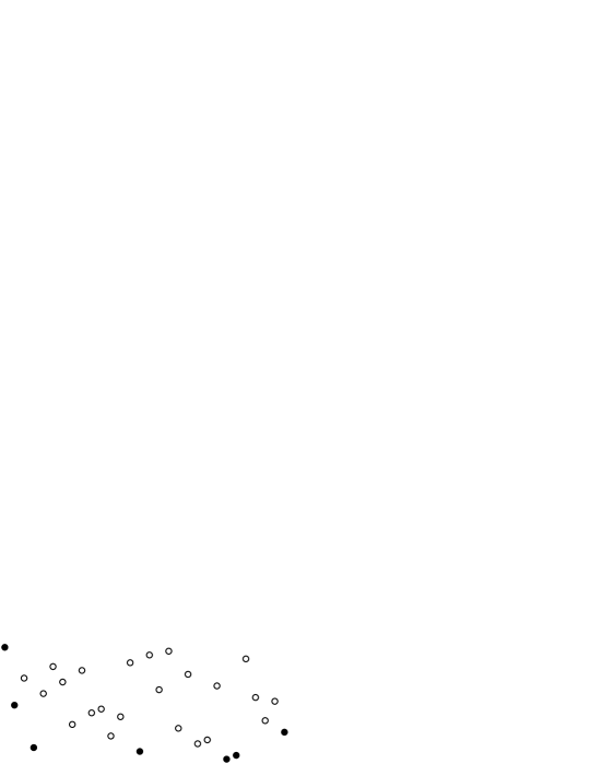
Figure 1. A random total order $\lhd$ of the interval $[1,30]$, with founders shown as filled discs, and other elements as unfilled discs.

In the iterative description for the WI model on $[1,n]$, the founders are the indices $i$ at which the color $X_{i}$ was inserted at an endpoint of the interval during the relevant insertion step (including the case of the first color to be chosen). An immediate consequence is that the law of the random WI order $\lhd$ on $[1,n]$ is given by

(6) $$\mathbb{P}(\lhd=\triangleleft)=\frac{w^{|\mathcal{F}(\triangleleft)|}}{Z(w,n)},$$

where $\triangleleft$ is any of the $n!$ deterministic total orders on $[1,n]$, and $Z(w,n)$ is an appropriate normalizing constant.

Our next goal is to prove the following analogue of Proposition 6 for WI orders. This time, $w=1$ is the attracting fixed point.

Proposition 8.

Fix $w>0$ and $m\geq 1$. For $n>m$, let $\lhd^{n}$ be WI order on $[-n,n]$. As $n\to\infty$, the restriction $\lhd^{n}|_{[-m,m]}$ converges in law to a uniformly random total order on $[-m,m]$.

The following is the only estimate that we need in this section.

Lemma 9.

Fix $w>0$ and $n\geq 1$, and let $\lhd^{[n]}$ be WI order with weight $w$ on $[1,n]$. If $n/3<k<2n/3$ then

$$\mathbb{P}\bigl{(}k\in\mathcal{F}(\lhd^{[n]})\bigr{)}<\frac{c\log n}{n},$$

where $c$ is a constant depending only on $w$.

Proof.

Fix $w$, and write $p_{n,k}:=\mathbb{P}(k\in\mathcal{F}(\lhd^{[n]}))$. By symmetry we have $p_{n,n+1-k}=p_{n,k}$, and $p_{n,1}=p_{n,n}=1$ since the endpoints of an interval are always founders. Considering the last step of the insertion procedure gives the recurrence

$$p_{n+1,k}=\frac{1}{2w+n-1}\bigl{[}(w+k-2)p_{n,k-1}+(w+n-k)p_{n,k}\bigr{]}$$

for $2\leq k\leq n$. (Here the two terms on the right reflect the possibilities that the insertion is before, of after, location $k$; if the insertion is at $k$ then $k$ is not a founder). A straightforward induction then shows that $p_{n,k}$ is unimodal in $k$:

(7) $$p_{n,k}\geq p_{n,k+1},\quad k<\tfrac{n}{2}.$$

On the other hand, writing $s_{n}:=\sum_{i}p_{n,i}=\mathbb{E}|\mathcal{F}(\lhd^{[n]})|$, we obtain similarly $s_{1}=1$ and

$$s_{n+1}=s_{n}+\frac{2w}{2w+n-1},$$

and hence

(8) $$s_{n}\leq c_{1}\log n$$

for some $c_{1}=c_{1}(w)$.

Now if $n/3<k<2n/3$ then (8) and (7) give

$$c_{1}\log n\geq s_{n}\geq\sum_{i=1}^{\lceil n/3\rceil}p_{n,i}\geq\tfrac{n}{3}\,p_{n,\lceil n/3\rceil},$$

so $p_{n,\lceil n/3\rceil}\leq(3c_{1}\log n)/n$, and the result follows from (7). ∎

Corollary 10.

Fix $w>0$ and $m\geq 1$. For $n\geq m$, let $\lhd^{n}$ be the WI order with weight $w$ on $[-n,n]$. We have

$$\mathbb{P}\bigl{(}\mathcal{F}(\lhd^{n})\cap[-m,m]=\emptyset)\to 1\qquad\text{as }n\to\infty.$$

Proof.

This follows from Lemma 9 by a union bound. ∎

Lemma 11.

Fix $w>0$, and integer intervals $[a,b]\subseteq[A,B]$. Let $\lhd$ be the WI order on $[A,B]$. Given the event $\mathcal{F}(\lhd)\cap[a,b]=\emptyset$, the conditional law of the restriction $\lhd|_{[a,b]}$ is the uniform measure on total orders of $[a,b]$.

Proof.

Consider the representation (6) of the law of $\lhd$. Let $\triangleleft_{1},\triangleleft_{2}$ be two total orders on $[a,b]$ that differ by a single transposition. The two events

$$\bigl{\{}\mathcal{F}(\lhd)\cap[a,b]=\emptyset,\;\lhd|_{[a,b]}=\triangleleft_{i}\bigr{\}},\qquad i=1,2$$

correspond to two (disjoint) sets of total orders on $[A,B]$. There is an explicit bijection between these sets that preserves the set of founders: we simply exchange the positions of the two transposed elements of $[a,b]$ within the order on $[A,B]$. ∎

Proof of Proposition 8.

This is an immediate consequence of Corollaries 10 and 11. ∎

We now shift our focus to the conditional law of the WI coloring given the total order. For a total order $\triangleleft$ on an interval $[a,b]$, define functions $L=L_{\triangleleft}$ and $R=R_{\triangleleft}$ on $[a,b]$ by

(9) $$L(i) :=\max\{j<i:j\triangleleft i\};$$

$$R(i) :=\min\{j>i:j\triangleleft i\},$$

where $\min\emptyset=\max\emptyset:=\infty$. Note that the founders of $\triangleleft$ are the elements $i$ for which $L(i)$ or $R(i)$ is infinite.

By considering the insertion procedure for the WI model on $[a,b]$, we seethat the conditional law of the coloring given the order $\lhd$ can be expressed as follows. We assign colors to the elements of $[a,b]$ one by one, in the order $\lhd$. Conditional on the previous choices, the color $X_{i}$ assigned to $i$ is chosen uniformly at random from the set

$$[q]\setminus\{X_{L(i)},X_{R(i)}\}.$$

(The set has size $q$ at the first step, and subsequently has size $q-1$ if $i$ is a founder, and otherwise $q-2$. Of course, $L(i)$ and $R(i)$ correspond to the neighbors of $i$ when it was inserted.)

The above sequential coloring may be done in other orders. Specifically, consider the directed graph $G=G(\lhd)$ with vertex set $[a,b]$ and with edges from $i$ to $L(i)$, and from $i$ to $R(i)$, for each $i$, wherever these quantities are finite. There is a partial order $\prec$ on $[a,b]$ generated by the set of inequalities $\{i\succ j:G\text{ has an edge from }i\text{ to }j\}$. Then the above sequential coloring procedure may be done in any order that is a linear extension of $\prec$. The resulting conditional law is the same for all such linear extensions.

The graph $G$, and a coloring, are illustrated in Figure 2. It is helpful to draw vertex $i$ with horizontal coordinate $i$ and vertical coordinate given by its position in $\lhd$, as before. Then $G$ has a “lower” path composed of all the founders, with edges directed inwards along the path towards the earliest element in the order. On each edge of this path, there is a structure built of triangles, each with its base on an existing edge (starting with the edge of the path) and its apex above that edge.

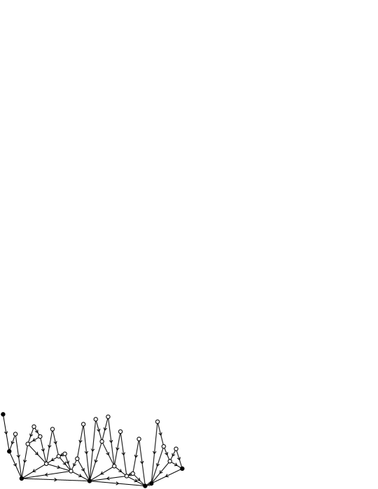
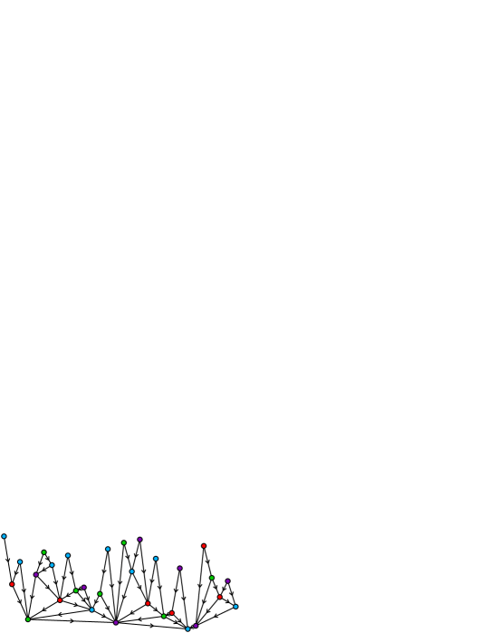
Figure 2. Top: the directed graph $G$ corresponding to a random total order on the interval $[1,30]$. Founders are shown as filled discs. Middle: A $4$-coloring of $G$. Bottom: The resulting $4$-coloring of the interval.

The conditional law has the following Markovian property.

Lemma 12.

Fix $q\geq 3$, and consider integer intervals $[a,b]\subseteq[A,B]$. Let $\triangleleft,\triangleleft\,^{\prime}$ be deterministic total orders on $[A,B]$, and let $X,X^{\prime}$ be random colorings on $[A,B]$ chosen according to the respective conditional laws given $\triangleleft,\triangleleft\,^{\prime}$ under the WI model with $q$ colors. Suppose that:

• $\triangleleft|_{[a,b]}=\triangleleft\,^{\prime}|_{[a,b]}$, and

• $\mathcal{F}(\triangleleft|_{[a,b]})=\{a,b\}$.

Then $X|_{[a,b]}\stackrel{{\scriptstyle d}}{{=}}X^{\prime}|_{[a,b]}$.

Proof.

The proof is illustrated in Figure 3. Let $G,G^{\prime}$ be the directed graphs on $[A,B]$ corresponding to $\triangleleft,\triangleleft\,^{\prime}$. Condition (ii) implies that $G$ has an edge between $a$ and $b$ (in some direction), and that for all $i\in(a,b)$ we have $i\,\triangleright a$ and $i\,\triangleright b$. Therefore, the subgraph of $G$ induced by $[a,b]$ includes all the edges of $G$ that are incident to $(a,b)$, and no edges out of $\{a,b\}$ except the edge connecting them. By symmetry under permutations of $[q]$, the joint law $(X_{a},X_{b})$ must be uniform on the set of $q^{2}-q$ ordered pairs of unequal colors. By (ii), all the same observations apply to $G^{\prime}$, and the subgraphs of $G,G^{\prime}$ induced by $[a,b]$ are identical. By the sequential coloring procedure described above, the conditional law of $X|_{(a,b)}$ given $(X_{a},X_{b})$ is thus identical to its counterpart for $X^{\prime}$, concluding the proof. ∎

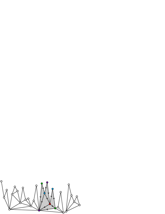
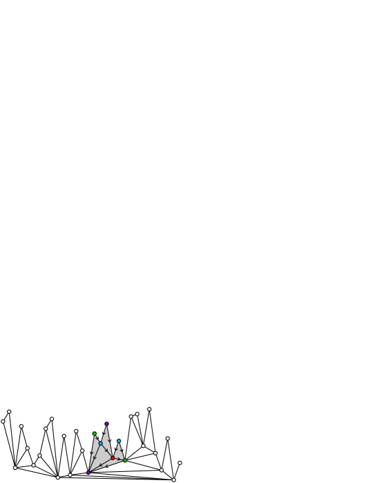
Figure 3. An illustration of Lemma 12 and its proof. The directed graphs associated with two different orders on the interval are shown. The restrictions to the highlighted subinterval agree, and the only founders of the restricted order are the endpoints. Therefore the conditional laws of the colorings agree on the subinterval.

Corollary 13.

Fix $q\geq 3$, and consider integer intervals $[a,b]\subseteq[A,B]\subseteq[\mathcal{A},\mathcal{B}]$. Let $\triangleleft,\triangleleft\,^{\prime}$ be deterministic total orders on $[\mathcal{A},\mathcal{B}]$, and let $X,X^{\prime}$ be random colorings chosen according to their respective conditional laws. Suppose that:

• $\triangleleft|_{[A,B]}=\triangleleft\,^{\prime}|_{[A,B]}$, and

• $\mathcal{F}(\triangleleft|_{[A,B]})\cap[a,b]=\emptyset$.

Then $X|_{[a,b]}\stackrel{{\scriptstyle d}}{{=}}X^{\prime}|_{[a,b]}$.

Proof.

Write $\triangleleft\,_{0}:=\triangleleft|_{[A,B]}$. Define $[c,d]$ to be the minimal interval between founders of $\triangleleft\,_{0}$ that contains $[a,b]$. I.e. let $c:=\max\{\mathcal{F}(\triangleleft\,_{0})\cap[A,a-1]\}$ and $d:=\min\{\mathcal{F}(\triangleleft\,_{0})\cap[b+1,B]\}$ (which must be finite because the endpoints $A,B$ are founders of any order on $[A,B]$). Then $\mathcal{F}(\triangleleft\,_{0})\cap[c,d]=\{c,d\}$, which implies that $i\triangleright_{0}c$ and $i\triangleright_{0}d$ for all $i\in(c,d)$, and thus $\mathcal{F}(\triangleleft|_{[c,d]})=\{c,d\}$. Now we can apply Lemma 12 to obtain $X|_{[c,d]}\stackrel{{\scriptstyle d}}{{=}}X^{\prime}|_{[c,d]}$, whence $X|_{[a,b]}\stackrel{{\scriptstyle d}}{{=}}X^{\prime}|_{[a,b]}$. ∎

We can now prove the main result of this section.

Proof of LABEL:{limit-col}.

Let $\epsilon>0$. By Corollary 10 with weight $1$, choose $M=M(m)>m$ sufficiently large that a uniformly random order on $[-M,M]$ has no founders in $[-m,m]$ with probability at least $1-\epsilon$. Now, by Proposition 8, choose $n=n(M)>M$ sufficiently large that for both set of parameters $(q,w)$ and $(q,w^{*})$, the restriction of the WI order on $[-n,n]$ to $[-M,M]$ differs from the uniform total order on $[-M,M]$ by at most $\epsilon$ in total variation.

Let $(X,\lhd)$ and $(X^{*},\lhd^{*})$ be WI models on $[-n,n]$ with respective parameters $(q,w)$ and $(q,w^{*})$. We will couple them in such a way that their colorings agree on $[-m,m]$ with high probability. First, by the choice of $n$, couple $\lhd$ and $\lhd^{*}$ so that, conditional on some event $E$ of probability at least $1-\epsilon$, we have that $\lhd|_{[-M,M]}=\lhd^{*}|_{[-M,M]}$, and this restriction is conditionally uniformly random. By the choice of $M$, on some further event $E^{\prime}\subseteq E$ with $\mathbb{P}(E^{\prime}\mid E)\geq 1-\epsilon$ (and thus $\mathbb{P}(E^{\prime})\geq(1-\epsilon)^{2}$), the restriction $\lhd|_{[-M,M]}$ has no founders in $[-m,m]$. Now, by Corollary 13, we can couple $X$ and $X^{*}$ (with the correct conditional laws given $\lhd$ and $\lhd^{*}$) so that on $E^{\prime}$ we have $X|_{[-m,m]}\stackrel{{\scriptstyle d}}{{=}}X^{*}|_{[-m,m]}$.

However, the consistency property in Proposition 4 implies that $X^{*}|_{[-m,m]}$ is equal in law to the WI coloring with parameters $(q,w^{*})$ on $[-m,m]$, for all $n$. ∎

5. Proof of main result

Proof of Theorem 1.

Let $q=4$, let $(U_{i},\phi_{i})_{i\in\mathbb{Z}}$ be as in Proposition 2, and let $X=(X_{i})_{i\in\mathbb{Z}}$ be the solution to (1). By Proposition 2, it suffices to show that $(X_{i})_{i\in\mathbb{Z}}$ is equal in law to the $1$-dependent $4$-coloring constructed in [4]. By Propositions 4 and 5, this will follow if we can show that its restriction to the interval $[-m,m]$ is equal in law to the WI model with weight $w^{*}(4)=3/2$, for every $m$.

Let $\lhd$ be the total order on $\mathbb{Z}$ induced by $(U_{i})_{i\in\mathbb{Z}}$; i.e. let $i\lhd j$ if and only if $U(i)<U(j)$. Let $n\geq 1$ be an integer, let $\lhd^{n}$ be the restriction $\lhd|_{[-n,n]}$, and let define the neighbor maps $L^{n}=L_{\lhd^{n}}$ and $R^{n}=R_{\lhd^{n}}$ via (9), so that $L^{n}(i)$ or $R^{n}(i)$ is infinite when $i$ is a founder of $\lhd^{n}$. Now define a coloring $X^{n}=(X_{-n},\ldots,X_{n})$ to be the solution of (1), except restricted to $i\in[-n,n]$, and using $L^{n},R^{n}$ in place of $L,R$. We take $X_{\infty}:=\infty$, so that when $L^{n}(i)$ or $R^{n}(i)$ is infinite, the restriction involving $X_{L^{n}(i)}$ or $X_{R^{n}(i)}$ in (1) is ignored. Existence and uniqueness of the solution is clear by considering the integers $i\in[-m,m]$ in the order $\lhd$.

Since the preference orders $\phi_{i}$ are uniformly random, $X^{n}$ is equal in law to the WI coloring on $[-n,n]$ with $4$ colors and weight $w=1$. On the other hand, let $n>m$, and let $G_{n}$ be the event that there exist lucky integers $A,B$ with $[-m,m]\subseteq[A,B]\subseteq[-n,n]$ and $i\rhd A,B$ for all $i\in(A,B)$. Then by the argument in the proof of Proposition 2, $X^{n}|_{[-m,m]}$ and $X|_{[-m,m]}$ are equal on $G_{n}$ (where $X=(X_{i})_{i\in\mathbb{Z}}$ is the global solution to (1) mentioned earlier). Lemma 3 implies that a.s. $G_{n}$ occurs eventually as $n\to\infty$. Therefore $X^{n}|_{[-m,m]}\to X|_{[-m,m]}$ a.s. But Proposition 6 states that $X^{n}|_{[-m,m]}$ converges in law to the WI coloring $Y$ with weight $w^{*}$ on $[-m,m]$, so $X|_{[-m,m]}\stackrel{{\scriptstyle d}}{{=}}Y$ as required. ∎

References

- [1] J. Aaronson, D. Gilat, M. Keane, and V. de Valk. An algebraic construction of a class of one-dependent processes. Ann. Probab., 17(1):128–143, 1989.
- [2] A. Borodin, P. Diaconis, and J. Fulman. On adding a list of numbers (and other one-dependent determinantal processes). Bull. Amer. Math. Soc. (N.S.), 47(4):639–670, 2010.
- [3] R. Durrett. Probability: theory and examples. Cambridge Series in Statistical and Probabilistic Mathematics. Cambridge University Press, Cambridge, fourth edition, 2010.
- [4] A. E. Holroyd and T. M. Liggett. Finitely dependent coloring. 2014. arXiv:1403.2448.
- [5] A. E. Holroyd and T. M. Liggett. Symmetric 1-dependent colorings of the integers. 2014. arXiv:1407.4514.
- [6] A. E. Holroyd, O. Schramm, and D. B. Wilson. Finitary coloring. 2008. Manuscript. Final version in preparation.
- [7] S. Janson. Runs in -dependent sequences. Ann. Probab., 12(3):805–818, 1984.
- [8] N. Linial. Distributive graph algorithms – global solutions from local data. In 28th Annual Symposium on Foundations of Computer Science, pages 331–335. IEEE, 1987.
- [9] M. Naor. A lower bound on probabilistic algorithms for distributive ring coloring. SIAM J. Discrete Math., 4(3):409–412, 1991.