Optimal Redshift Weighting For Baryon Acoustic Oscillations

Abstract

Future baryon acoustic oscillation (BAO) surveys will survey very large volumes, covering wide ranges in redshift. We derive a set of redshift weights to compress the information in the redshift direction to a small number of modes. We suggest that such a compression preserves almost all of the signal for most cosmologies, while giving high signal-to-noise measurements for each combination. We present some toy models and simple worked examples. As an intermediate step, we give a precise meaning to the “effective redshift” of a BAO measurement.

1 Introduction

The baryon acoustic oscillation (BAO) method has now become an essential component of the dark energy toolbox by mapping the expansion history of the Universe (see Weinberg et al., 2013; Mortonson et al., 2014, for recent reviews). Current sets of surveys (Blake et al., 2012; Anderson et al., 2014) have achieved distance accuracies at the per cent level when averaged across relatively wide redshift bins; the next generation of surveys (Sugai et al., 2012; Levi et al., 2013; Laureijs et al., 2011; Spergel et al., 2013) aim to improve both the redshift resolution and the redshift range of these measurements. This paper aims to develop techniques to robustly map the distance-redshift relation for these surveys.

Conceptually, one can improve the resolution of the reconstructed distance-redshift relation by splitting samples into narrower redshift bins and repeating the traditional analysis on these. However, such a procedure has a significant disadvantage for BAO measurements: the robustness of the BAO technique derives from focusing only on the BAO feature in the correlation function or power spectrum, marginalizing over the broadband shape. A reliable measurement of distances therefore requires a significant detection of the BAO feature in the correlation function and low signal-to-noise detections can lead to very non-Gaussian likelihood functions for the inferred distance (eg. Blake et al., 2012; Xu et al., 2013) Splitting samples into multiple bins exacerbates this problem. Binning also has other disadvantages: the choice of bins is often arbitrary and splitting a sample into completely disjoint bins loses signal across bin boundaries unless a large number of cross-spectra are included. While some of these disadvantages may be overcome, they can add significantly to the complexity of the analysis.

Rather than breaking the sample into multiple redshift slices, we instead seek a compression of the information in the redshift direction onto a small number of ‘modes’, or weighted integrals. This allows us to work with relatively wide redshift bins while retaining sensitivity to evolution of the distance-redshift relation and gives a firm meaning to the ‘effective redshift’ of the sample. Our approach is reminiscent of principal component analysis or optimal subspace filtering, though being technically somewhat different.

To do so, we start by parametrizing the distance redshift relation relative to a fiducial choice of cosmology (see Percival et al. (2007) for related efforts to fit a distance redshift relation using BAO measurements). We demonstrate that simple parametrizations capture a broad range of possible distance redshift relations over wide redshift intervals. Given a particular choice of parametrization, we then derive appropriate weighted integrals (in redshift) of the correlation function that are (under particular assumptions) optimal estimates of the parameters in the distance-redshift relation. These integrals may be thought of as generalizations of simple redshift bins, designed to efficiently combine the information at different redshifts.

While we argue in this paper for a model-agnostic parametrization, different choices may be more appropriate for more specific applications. For instance, one may choose the equation of state of dark energy to parametrize the distance-redshift relation. The modes would then be different from the ones we focus on for much of the presentation, but the overall approach would remain unchanged. We give a simple example later to illustrate this flexibility.

The outline of this paper is as follows. We introduce our parametrization of the distance-redshift relation in section 2, showing that it fits a wide range of cosmologies to the sub per cent level. Section 3 introduces the weighted correlation functions and our optimal weights, including a toy model to demonstrate the improvements that can be expected by weighting. Section 4 specializes our discussion to the case of BAO and describes a possible implementation of the method. We conclude in section 5 with a discussion of our results and directions for future development. Some technical details are relegated to an appendix.

2 Parametrizing the Distance Redshift Relation

We begin by parametrizing the distance-redshift relation as a small fluctuation about a fiducial relation. This scheme is standard in BAO studies, as one typically uses a fiducial cosmology to convert the angular positions and redshifts of the galaxies into 3D positions before measuring the clustering signal. Motivated by inflation and supported by recent observations (Planck Collaboration et al., 2013; Anderson et al., 2014) we shall assume throughout that the spatial hypersurfaces are flat, and we shall denote the comoving radial distance as $\chi$.

We choose a pivot redshift $z_{0}$ within the redshift range of a planned survey and denote the fiducial comoving distance at $z_{0}$ by $\chi_{f,0}$. We defer the reader to the end of this section for a discussion about the choice of $z_{0}$, while merely pointing out the analysis below doesn’t depend on a particular choice of $z_{0}$. We model the true distance-redshift relation $\chi(z)$ as

$$\frac{\chi(z)}{\chi_{f}(z)}=\alpha_{0}\left(1+\alpha_{1}x+\frac{1}{2}\alpha_{2}x^{2}\right)$$ (1)

where $1+x\equiv\chi_{f}(z)/\chi_{f,0}$. The parameters $\alpha_{0}$, $\alpha_{1}$ and $\alpha_{2}$ are specified by matching the distance-redshift relation and its derivatives at $z_{0}$ :

$$\alpha_{0} =\frac{\chi_{0}}{\chi_{f,0}}$$ (2)

$$\alpha_{1} =\frac{H_{f,0}\chi_{f,0}}{H_{0}\chi_{0}}-1$$ (3)

$$\alpha_{2} =(1+\alpha_{1})\chi_{f,0}\left[H^{\prime}_{f,0}-\alpha_{0}(1+\alpha_{1})H^{\prime}_{0}\right]-2\alpha_{1}$$ (4)

where $H^{\prime}_{f,0}=H^{\prime}_{f}(z_{0})$ and $H^{\prime}_{0}=H^{\prime}(z_{0})$. An explicit calculation of $\alpha_{1}$ and $\alpha_{2}$ is in the appendix.

Figure 1: The fractional error in our proposed distance parametrization for three example cosmologies. The fiducial cosmology here is a flat $\Lambda$CDM cosmology with $\Omega_{M}=0.274$ and $h=0.7$. The solid [red] line is an $\Omega_{M}=0.2$, $h=0.7$ cosmology; the short dashed line is our fiducial cosmology with a dark energy equation of state $w=-0.7$, and the dotted [green] line corresponds to $\Omega_{M}=1$ and $h=1$. The pivot redshift, $z_{0}=1.08$ is the effective redshift of the redshift range between $z=0.5$ and $1.5$, similar to the the redshift coverage of planned redshift surveys like DESI and Euclid.

Figure 2: The same as Fig. 1 except now showing the error in the Hubble parameter $H(z)=1/\chi^{\prime}(z)$. The errors in the plot are larger, reflecting the fact that our approximation is first order for $H$, albeit being second order for $\chi$.

Figure 3: The impact of changing $z_{0}$ on the distance redshift relation. The fiducial cosmology here is the same as the previous two figures, while the true cosmology has $\Omega_{M}=0.3$, $h=0.7$ and $w=-1$. The dashed [blue] line assumes $z_{0}=1.08$ (equal to the effective redshift), the solid [red] line corresponds to $z_{0}=0.75$, while the dotted [green] line assumes $z_{0}=1.25$. The reconstructed distance-redshift relations all agree to better than 0.02 per cent over the entire redshift range.

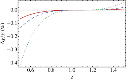
This parametrization to the second order can recover the distance-redshift relation to sub-percent levels across a wide range of redshifts and cosmologies. Fig. 1 displays the fractional error in the parametrization between $z=0.5$ and $1.5$ for three example cosmologies. These span a wide range of cosmological parameters and are not meant to represent currently viable models. Even for the extreme $\Omega_{M}=1$ case, the error is less than $0.5\%$ over the entire redshift range.

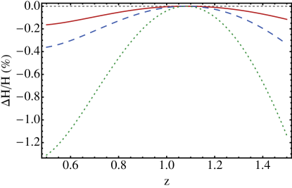
Fig. 2 shows a similar plot of the fractional error in the Hubble parameter $H(z)=1/\chi^{\prime}(z)$. A second order approximation in distance translates to a first order one in $H$ and explains the larger errors. Despite that, for cosmologies close to the fiducial model, the accuracy is still at the sub-percent level.

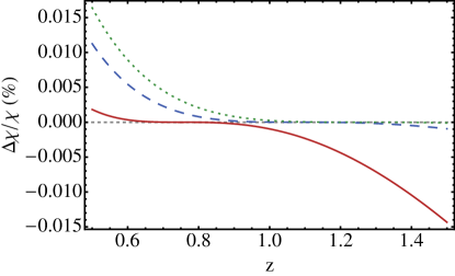
It is worth noting at this point that $z_{0}$ is a meta-parameter which can be chosen for convenience, rather than a property of the sample under consideration. For best results the fiducial redshift should be chosen close to the center of the redshift range, for example at the ‘effective’ or pair-weighted redshift of the sample. Fig. 3 highlights this freedom in the choice of $z_{0}$, demonstrating that the reconstructed distance-redshift relations in each of these cases agree to better than 0.02 per cent, much smaller than the expected statistical uncertainty in these measurements.

3 Optimal Weights

3.1 Derivation

We start by deriving the general formalism for optimal linear weights. The derivation is modeled on Tegmark et al. (1997); we summarize it here for completeness, while specializing to the particular problem at hand. Imagine measuring the correlation function in $n$ $z$-bins. The uncompressed correlation function data vector is

$$\boldsymbol{\Xi}(r)=\left(\begin{array}[]{c}\xi(r,z_{1})\\ \xi(r,z_{2})\\ \vdots\\ \xi(r,z_{n})\end{array}\right)$$ (5)

Weighting the redshift slices by the $n$-dimensional vector $\boldsymbol{w}^{t}=\left(w_{1},w_{2},\cdots,w_{n}\right)$, we linearly compress the data into one single $z$-bin according to these weights.

$$\xi_{w}(r)=\boldsymbol{w}^{t}\boldsymbol{\Xi}(r)$$ (6)

where $\xi_{w}$ is the weighted correlation function. The mean and covariance $\boldsymbol{C}_{w}$ of the compressed data are

$$\langle\xi_{w}(r)\rangle =\boldsymbol{w}^{t}\langle\boldsymbol{\Xi}(r)\rangle$$ (7)

$$\langle\xi_{w}(r)\xi_{w}^{t}(r)\rangle-\langle\xi_{w}(r)\rangle\langle\xi_{w}^{t}(r)\rangle =\boldsymbol{w}^{t}\boldsymbol{C}\boldsymbol{w}$$ (8)

where $\boldsymbol{C}$ is an $n\times n$ matrix and $\boldsymbol{C}_{w}=\boldsymbol{w}^{t}\boldsymbol{C}\boldsymbol{w}$ is a scalar. We write our model correlation functions at distance $r$ in different $z$-bins $\boldsymbol{M}(r)$ in the same format as $\boldsymbol{\Xi}$. Using the redshift weights $\boldsymbol{w}$, we linearly compress the model correlation function data in the same fashion,

$$m(r)=\boldsymbol{w}^{t}\boldsymbol{M}(r)$$ (9)

The model correlation function depends on parameters $\boldsymbol{\Theta}=\left\{\theta_{1},\theta_{2},\cdots\right\}$. Restricting to a single unknown parameter, the error on $\theta_{i}$ is $\left(\mathcal{F}_{ii}\right)^{-1/2}$, where $\mathcal{F}_{ii}$ is the $i$-th diagonal element of the Fisher information matrix. This is given by

$$\mathcal{F}_{ii}=m_{,i}^{t}\boldsymbol{C}_{w}^{-1}m_{,i}$$ (10)

where $m_{,i}$ is the derivative of the model correlation function $m$ with respect to parameter $\theta_{i}$. Since $\boldsymbol{C}_{w}$ is a scalar,

$$\mathcal{F}_{ii}=\frac{m_{,i}^{t}m_{,i}}{\boldsymbol{w}^{t}\boldsymbol{C}\boldsymbol{w}}=\frac{\boldsymbol{w}^{t}\boldsymbol{M}_{ii}\boldsymbol{w}}{\boldsymbol{w}^{t}\boldsymbol{C}\boldsymbol{w}}$$ (11)

where $\boldsymbol{M}_{ij}=\boldsymbol{M}_{,i}\boldsymbol{M}_{,j}^{t}$ is an $n\times n$ matrix. Our goal is to find the weights that minimize the error of $\theta_{i}$, and therefore maximize $\mathcal{F}_{ii}$.

Since $\mathcal{F}_{ii}$ is unchanged under a rescaling of $\boldsymbol{w}$, we constrain $\boldsymbol{w}^{t}\boldsymbol{C}\boldsymbol{w}=1$ for convenience. Introducing a Lagrange multiplier $\lambda$, we maximize

$$\mathcal{G}=\boldsymbol{w}^{t}\boldsymbol{M}_{ii}\boldsymbol{w}-\lambda\left(\boldsymbol{w}^{t}\boldsymbol{C}\boldsymbol{w}-1\right).$$ (12)

Setting the gradient of $\mathcal{G}$ with respect to $\boldsymbol{w}$ to zero yields

$$\boldsymbol{M}_{ii}\boldsymbol{w}=\lambda\boldsymbol{C}\boldsymbol{w}$$ (13)

Using $\boldsymbol{M}_{ii}\boldsymbol{w}=\boldsymbol{M}_{,i}\boldsymbol{M}_{,i}^{t}\boldsymbol{w}$ and as $\boldsymbol{M}_{,i}^{t}\boldsymbol{w}$ is a scalar, we have

$$\boldsymbol{C}\boldsymbol{w}\propto\boldsymbol{M}_{,i}\,.$$ (14)

so that the weights are (up to normalizations)

$$\boldsymbol{w}=\boldsymbol{C}^{-1}\boldsymbol{M}_{,i}\,.$$ (15)

For these weights, the Fisher matrix is

$$\mathcal{F}_{ii}=\boldsymbol{M}_{,i}^{t}\boldsymbol{C}^{-1}\boldsymbol{M}_{,i}$$ (16)

while the error on $\theta_{i}$ is

$$\Delta\theta_{i}=\left(\boldsymbol{M}_{,i}^{t}\boldsymbol{C}^{-1}\boldsymbol{M}_{,i}\right)^{-1/2}.$$ (17)

It is worth noting that the Fisher matrix is identical to what we would have without any compression. Our compression is therefore theoretically lossless, and has extracted all the information in the original data.

3.2 A Toy Model

In order to build intuition for the results of the previous section, we first apply this to a toy model, which captures the essential aspects of the full BAO problem. We assume that the correlation function at a separation $x$ and redshift $z$ is a Gaussian

$$\xi(x,z)=\exp(-x^{2}).$$ (18)

We also assume that choosing an incorrect cosmology (here parameterized simply by $\alpha_{1}$) changes the separation $x\rightarrow x-\alpha_{1}z$, making the correlation redshift dependent

$$\xi(x)\rightarrow\xi\left(x-\alpha_{1}z\right)$$ (19)

Our goal is therefore to estimate $\alpha_{1}$ from observations of $\xi$.

There are three cases we consider. The first (“Full”) is where we imagine fitting to the correlation function in both $x$ and $z$; this captures all the information and should yield the most precise measurements. This would be equivalent to splitting the galaxy sample into infinitesimal redshift bins and fitting a full model to it, which is not possible for the real correlation function for the reasons described in Sec. 1. The second (“Unweighted”) is to integrate the two dimensional correlation function $\xi(x,z)$ along the $z$ axis to collapse it down to a one dimensional function $\xi_{\rm un}(x)\equiv\int dz\,\xi(x,z)$.

The third case (“Weighted”) is to construct the weighted combination $\xi_{\rm w}(x)\equiv\int dz\,w(z)\xi(x,z)$ where $w(z)$ are the weights computed in the previous section. We note that we only combine the data in the $z$ direction here, even though the formalism of the previous section would have allowed us to collapse in both $x$ and $z$. We do this because the shape of the true galaxy correlation function is uncertain (hence the marginalization over nuisance shape parameters). Furthermore, as written, the weights do not have any $x$ dependence. While not generic, this is explicitly true for our toy model (as described below). We also construct the weights for the actual correlation function (described in the next section) to have this property.

Figure 4: A demonstration of the efficiency of using optimal weights to compress information. We consider a toy model $\xi(r,z)=\exp(-(x-\alpha_{1}z)^{2})$, where $\alpha_{1}$ is the parameter to be fit. We consider three cases : (1) [x-axis] “Full” - where we fit the two-dimensional function $\xi(x,z)$, (2) [y-axis, top plot] “Unweighted” - where we fit $\int dz\,\xi(x,z)$, and (3) [y-axis, bottom plot] “Weighted” - where we fit $\int dz\,w(z)\xi(x,z)$ with $w(z)$ being the optimal weight. The figure summarizes the results of 500 simulations with the true value of $\alpha_{1}$ equal to 0 (see the text for more details). Both the unweighted and weighted approaches yield unbiased estimates. The weighted estimator is almost perfectly correlated with the full case, demonstrating negligible loss of information when compressing down to a single mode.

We can now derive the optimal redshift weights for $\alpha_{1}$. For simplicity, we will assume that the measurements of $\xi(x,z)$ have constant, uncorrelated errors. In this case, the weights are simply proportional to $d\xi_{x,z}/d\alpha_{1}$, giving

$$w(z)=-2z(x-\alpha_{1}z)\exp\left[-(x-\alpha_{1}z)^{2}\right]\,.$$ (20)

The above derivative does still depend on $\alpha_{1}$. We make the usual approximation that we are making small perturbations to our fiducial cosmology and set $\alpha_{1}=0$. If this were not true (i.e. the measured values of $\alpha_{1}$ were significantly different from 0), one would need to iterate using an improved estimate of the true cosmology. Substituting into the above equation, and using the fact that the normalization of the weights is arbitrary, we find the simple relation

$$w(z)=z\,.$$ (21)

This weighting makes physical sense; one wants to downweight measurements close to $z=0$, where the correlation function has little sensitivity to $\alpha_{1}$, and upweight the measurements as $z$ increases, where the sensitivity is greater. The optimal weight is nothing but a matched filter, tracing the redshift dependence of the signal.

In order to quantitatively explore the impact of these weights, we simulate this toy model on an $81\times 11$ grid in $x$ and $z$, with $x$ in $[-4,4]$ and $z$ in $[0,1]$, and add a Gaussian random error of $\sigma=0.1$ to each measurement of $\xi$. Note that the particular choice of the size of this error does not change any of the conclusions below. We verify this by repeating our experiments with $\sigma=1$ and find identical behaviour (except for the fact that $\alpha_{1}$ is more poorly measured overall). We simply sum along the $z$ direction weighting each measurement by $1$ and $z$ to obtain the corresponding unweighted and weighted simulations respectively. Since we assume the errors to be uncorrelated, the variances for the unweighted and weighted simulations are simply $11\sigma^{2}$ and $\sigma^{2}\sum_{i}z_{i}^{2}$ (where the $z_{i}$ are the redshifts at which the model is evaluated). We then estimate $\alpha_{1}$ by numerically minimizing $\chi^{2}$, which is the maximum likelihood estimator in this case.

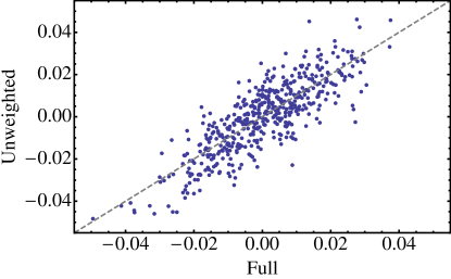
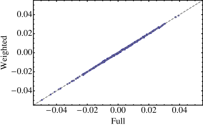
The results for 500 such simulations are summarized in Fig. 4. Each case yields an unbiased estimate for $\alpha_{1}$, but the unweighted estimator introduces an additional scatter to the full case. By contrast, the weighted estimator is almost perfectly correlated with the full case, compressing the data to one dimension with virtually no information loss. This highlights the usefulness and efficiency of using an optimal weighting scheme - the dimensionality of the data can be dramatically reduced with no loss of information.

4 Redshift Weighting for BAO

4.1 Preliminaries

Motivated by the results of the previous section, we turn to the construction of similar weights for BAO measurements. We lay out some basic preliminaries here, with the derivation in the next section. We will assume that the distance-redshift relation is parametrized as in Sec. 2.

In order to construct a redshift dependent model for the correlation function, we work in the plane parallel approximation and parametrize the effects of an incorrect choice of a distance-redshift relationship by an isotropic dilation ($\alpha(z)$) and an anisotropic warping ($\epsilon(z)$) parameter (Padmanabhan & White, 2008). However, unlike previous analyses which have used this parametrization, we will explicitly assume that these are redshift dependent (although we will often suppress this dependence for notational brevity). These distortion parameters can be related to stretching in the perpendicular and parallel directions by

$$r_{\parallel} =\alpha(1+\epsilon)^{2}r_{\parallel}^{\text{f}}$$ (22)

$$r_{\perp} =\alpha(1+\epsilon)^{-1}r_{\perp}^{\text{f}}$$ (23)

and the inverse relations by

$$\alpha =\left[\left(\frac{r_{\parallel}}{r_{\parallel}^{\text{f}}}\right)\left(\frac{r_{\perp}}{r_{\perp}^{\text{f}}}\right)^{2}\right]^{1/3}$$ (24)

$$\epsilon =\left(\frac{r_{\parallel}}{r_{\parallel}^{\text{f}}}\frac{r_{\perp}^{\text{f}}}{r_{\perp}}\right)^{1/3}-1\,.$$ (25)

In the plane parallel limit, we have

$$\frac{r_{\parallel}}{r_{\parallel}^{\text{f}}} =\frac{H_{f}(z)}{H(z)}$$ (26)

$$\frac{r_{\perp}}{r_{\perp}^{\text{f}}} =\frac{\chi(z)}{\chi_{f}(z)}$$ (27)

giving us

$$\alpha(z) =\left[\frac{H_{f}(z)\chi^{2}(z)}{H(z)\chi_{f}^{2}(z)}\right]^{1/3}$$ (28)

$$\epsilon(z) =\left[\frac{H_{f}(z)\chi_{f}(z)}{H(z)\chi(z)}\right]^{1/3}-1\,.$$ (29)

Using the definitions above, and the results from Sec. 2, we now relate $\alpha(z)$ and $\epsilon(z)$ to $\alpha_{0}$, $\alpha_{1}$ and $\alpha_{2}$. We get

$$\alpha =\left[\alpha_{0}\left(1+\alpha_{1}+\left(2\alpha_{1}+\alpha_{2}\right)x+\frac{3}{2}\alpha_{2}x^{2}\right)\right]^{1/3}$$ (30)

$$\cdot\left[\alpha_{0}\left(1+\alpha_{1}x+\frac{1}{2}\alpha_{2}x^{2}\right)\right]^{2/3}$$ (31)

$$\approx\alpha_{0}\left[1+\frac{1}{3}\alpha_{1}+\frac{1}{3}(4\alpha_{1}+\alpha_{2})x+\frac{5}{6}\alpha_{2}x^{2}\right]$$ (32)

and

$$1+\epsilon =\left[\alpha_{0}\left(1+\alpha_{1}+\left(2\alpha_{1}+\alpha_{2}\right)x+\frac{3}{2}\alpha_{2}x^{2}\right)\right]^{1/3}$$ (33)

$$\cdot\left[\alpha_{0}\left(1+\alpha_{1}x+\frac{1}{2}\alpha_{2}x^{2}\right)\right]^{-1/3}$$ (34)

$$\approx 1+\frac{1}{3}\alpha_{1}+\frac{1}{3}(\alpha_{1}+\alpha_{2})x+\frac{1}{3}\alpha_{2}x^{2}$$ (35)

where the approximations in the second line are obtained by only working to linear order in $\alpha_{1}$ and $\alpha_{2}$. We will also require the following partial derivatives (all evaluated at the fiducial value of $\alpha_{0}=1$, $\alpha_{1}=\alpha_{2}=0$ and denoted by subscript $0$)

$$\left.\frac{\partial\alpha}{\partial\alpha_{0}}\right|_{0} = 1 \left.\frac{\partial\epsilon}{\partial\alpha_{0}}\right|_{0} = 0$$ (36)

$$\left.\frac{\partial\alpha}{\partial\alpha_{1}}\right|_{0} = \frac{1}{3}(1+4x) \left.\frac{\partial\epsilon}{\partial\alpha_{1}}\right|_{0} = \frac{1}{3}(1+x)$$ (37)

$$\left.\frac{\partial\alpha}{\partial\alpha_{2}}\right|_{0} = \frac{1}{6}(2x+5x^{2}) \left.\frac{\partial\epsilon}{\partial\alpha_{2}}\right|_{0} = \frac{1}{3}(x+x^{2})$$ (38)

4.2 Derivation

As was laid out in Sec. 3.1, we compress the correlation multipoles $\xi_{\ell}(r,z)$ along the $z$ direction. The optimal weights are proportional to $\boldsymbol{C}\left[\xi_{\ell}(r,z_{1}),\xi_{\ell}(r,z_{2})\right]^{-1}\xi_{\ell,i}$ where $i$ runs over the parameters $\alpha_{0}$, $\alpha_{1}$ and $\alpha_{2}$. Note that we do not consider mixing in the $r$ or $\ell$ directions, to avoid building in sensitivity to the model of the correlation function.

To compute $\xi_{\ell,i}$, we need the dependence of the correlation function on $\alpha$ and $\epsilon$ (Padmanabhan & White, 2008; Xu et al., 2013) :

$$\xi_{0}(r) \rightarrow\xi_{0}(r)+(\alpha-1)\frac{d\xi_{0}(r)}{d\log r}$$ (39)

$$\xi_{2}(r) \rightarrow 2\epsilon\frac{d\xi_{0}(\alpha r)}{d\log r}$$ (40)

$$=2\epsilon\left[\frac{d\xi_{0}(r)}{d\log r}+(\alpha-1)\frac{d^{2}\xi_{0}(r)}{d(\log r)^{2}}\right]$$ (41)

Note that in the above, we set the intrinsic quadrupole correlation function $\xi_{2}$ to zero. We make this approximation motivated by the fact that we are interested in distance measurements from the BAO feature, which is very weak in the quadrupole. The derivatives of the correlation function are then simply given by

$$\xi_{0,i} =\alpha_{,i}$$ (42)

$$\xi_{2,i} =\epsilon_{,i}$$ (43)

where we have dropped all non-redshift dependent proportionality constants. We also note that the derivatives are all evaluated at the fiducial values of $\alpha=1$ and $\epsilon=0$.

Turning to the inverse covariance matrix, we note that the variance of a correlation function bin from a slice at redshift $z$ is schematically given by

$$C\sim\left(P+\frac{1}{\bar{n}}\right)^{2}\frac{1}{dV}$$ (44)

where

$$dV=\frac{\chi_{f}^{2}(z)}{H_{f}(z)}dzd\Omega$$ (45)

is the volume of slice being considered, $\bar{n}$ is the (redshift dependent) number density and $P$ is a measure of the power on scales corresponding to the bin in question. Again, since we’re focusing on the BAO feature, we will ignore the scale dependence in $P$ and simply treat it as a single number determined by the approximate scale corresponding to the BAO feature $(k\sim 0.1h\rm{Mpc}^{-1})$. We make the further simplifying assumption that the different redshift slices are independent, making the covariance matrix diagonal and trivial to invert:

$$d{\cal W}(z)\equiv C^{-1}=\left(\frac{\bar{n}}{\bar{n}P+1}\right)^{2}dV$$ (46)

This assumption simply means the weights are not strictly optimal, but will not bias the results. We observe this weighting is nothing but the commonly used FKP weights (Feldman et al., 1994) in galaxy surveys, a correspondence we make more explicit in Sec. 4.5. While the normalization of the weights is arbitrary, it is convenient to normalize the weights by the integral of the inverse covariance matrix over the survey

$$N=\int d{\cal W}\,.$$ (47)

We can now put together the different pieces to get our final results. We define the weighted correlation functions by $\xi_{w,\ell,i}$ :

$$\xi_{w,\ell,i}\equiv\frac{1}{N}\int\,d{\cal W}(z)\,w_{\ell,i}(z)\xi_{\ell}(z)$$ (48)

where, as before, $i$ runs over the distance-redshift parameters. The $w_{\ell,i}(z)$ are given by

$$w_{0,\alpha_{0}} = 1 w_{2,\alpha_{0}} = 0$$ (49)

$$w_{0,\alpha_{1}} = \frac{1}{3}(1+4x) w_{2,\alpha_{1}} = \frac{1}{3}(1+x)$$ (50)

$$w_{0,\alpha_{2}} = \frac{1}{6}(2x+5x^{2}) w_{2,\alpha_{2}} = \frac{1}{3}(x+x^{2})$$ (51)

Eq. 48 makes explicit that the overall redshift weights are the product of $w_{\ell,i}(z)$ and $d\mathcal{W}(z)$. We show two examples in Fig. 5. The top panel plots the weights for a constant $\bar{n}$ survey. The bottom panel is the same plot assuming a gaussian $\bar{n}$ centered around $z=1$. In a constant $\bar{n}$ survey, the weights for $\alpha_{0}$ are simply the inverse variance weights. The upward sloping weights curve suggest an upweight in the high redshift region of the survey. This is consistent with the intuition that slices at higher redshifts contain more volume and more galaxies, and thus smaller error bars, than those of lower redshifts.

4.3 Interpretation and Examples

Figure 5: Overall redshift weights for $\alpha_{0}$ and $\alpha_{1}$ in monopoles and quadrupoles of the two-point correlation function. We plot $w_{\ell,i}d\mathcal{W}$ throughout, although for brevity, the curves are simply labeled by $w_{\ell,i}$. The top panel assumes a constant $\bar{n}$ survey. The solid line is for $w_{0,\alpha_{0}}$ and is just the inverse variance weights, the dashed is $w_{0,\alpha_{1}}$ and the dotted is $w_{2,\alpha_{1}}$. The bottom panel assumes a gaussian $\bar{n}$ centered around $z=1$. The normalization of the weights is arbitrary. We have boosted the amplitudes of the weights for better visualization.

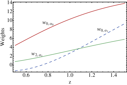
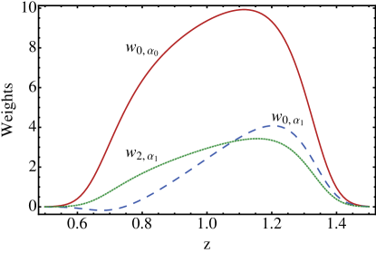
In order to develop some intuition for these weighted correlation functions, we consider the correlation function measured perpendicular to the line of sight; the case parallel to the line of sight is analogous. This case is simpler than the multipoles presented above, since it doesn’t mix the angular diameter distance and Hubble parameter measurements. In particular, we have

$$\xi_{\perp}(r)\rightarrow\xi_{\perp}(\alpha_{\perp}r)\sim\xi_{\perp}(r)+(\alpha_{\perp}-1)\frac{d\xi_{\perp}}{d\log r}$$ (52)

where

$$\alpha_{\perp}\equiv\frac{\chi(z)}{\chi_{f}(z)}=\alpha_{0}\left(1+\alpha_{1}x+\frac{1}{2}\alpha_{2}x^{2}\right)\,.$$ (53)

The corresponding weights are then

$$w_{\alpha_{0}} =1$$ (54)

$$w_{\alpha_{1}} =x$$ (55)

$$w_{\alpha_{2}} =x^{2}/2\,.$$ (56)

The weighted correlation functions can be schematically written as

$$\xi_{w}=A\xi_{\perp}+B\frac{d\xi_{\perp}}{d\log r}$$ (57)

where $A$ is just a normalization constant (independent of the values of $\alpha_{0}$, $\alpha_{1}$ and $\alpha_{2}$) and $B$ are integrals depending on the particular weights and $\alpha_{0}$, $\alpha_{1}$ and $\alpha_{2}$. The derivative term in the above equation is equivalent to a shift of the BAO feature. The different redshift weights result in different shifts for a given set of distance parameters. From these measured shifts, one can then infer the underlying parameters.

To make this example more concrete, we consider a redshift range defined by $-1\leq x\leq 1$ and assume the inverse variance weights are simply constant. The integrals are then trivial and are given by:

$$B_{\alpha_{0}} \propto 2\alpha_{0}+\frac{\alpha_{0}\alpha_{2}}{3}$$ (58)

$$B_{\alpha_{1}} \propto\frac{2}{3}\alpha_{0}\alpha_{1}$$ (59)

$$B_{\alpha_{2}} \propto\frac{1}{3}\alpha_{0}+\frac{1}{10}\alpha_{0}\alpha_{2}$$ (60)

where we have focused just on the shifts in the BAO feature. From the above, it is clear that given the measurements of three shifts, one can invert these to determine the $\alpha_{0}$, $\alpha_{1}$ and $\alpha_{2}$.

4.4 Alternate Parametrizations

Figure 6: The optimal weights to constrain the dark energy equation of state $w$, for the monopole ($w_{0}$ [red]) and the quadrupole ($w_{2}$ [blue]). We assume a survey with a constant number density. As before, the normalizations here are arbitrarily chosen for plotting convenience. The solid lines include the $d\mathcal{W}$ volume factor, while the dashed lines do not. The figure shows the relative importance of different redshifts to measuring $w$. At low redshifts, the weights are suppressed both due to the small volume, as well as the fact that all distance redshift relations tend to their Hubble law form $\chi=(c/H_{0})z$ independent of the equation of state. The impact of the volume factor with increasing redshift is also clearly evident. We note that this is an illustrative example; a complete treatment would include parameters beyond $w$.

Although we recommend our parametrization of the distance-redshift relation, the idea of optimal redshift weights is more general. To illustrate this, we consider a standard $w$CDM cosmology, with the Hubble parameter (and therefore, the distance-redshift relation) parametrized by a constant equation of state $w$ for dark energy :

$$H^{2}(z)=H_{0}^{2}\left[\Omega_{M}(1+z)^{3}+(1-\Omega_{M})(1+z)^{3(1+w)}\right]\,.$$ (61)

Since this is illustrative, we hold $H_{0}$ and $\Omega_{M}$ fixed; a full treatment would vary multiple parameters.

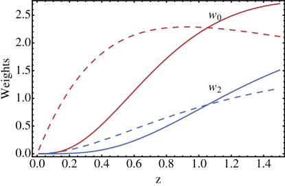
Proceeding as before, the weights will depend on derivatives of the monopole and quadrupole with $w$, which in turn, are proportional to derivatives of $\alpha(z)$ and $\epsilon(z)$ with $w$. Fig. 6 plots these weights for a survey with a constant number density of objects. The figure highlights the relative importance of different redshifts to measuring $w$. At low redshifts, the weights are suppressed both due to the small volume, as well as the fact that all distance redshift relations tend to their Hubble law form $\chi=(c/H_{0})z$ independent of the equation of state. The impact of the volume factor with increasing redshift is also clearly evident, upweighting the higher redshift regions even when the raw sensitivity to $w$ is flattening out (or decreasing).

4.5 Implementation Notes

We briefly discuss a possible implementation of this weighting scheme. We do not claim that this is a final implementation and we defer tests with mock catalogues to future work. Our goal here is to provide a proof-of-principle that such an implementation is both possible and straightforward.

We start with Eq. 48, and write the integral as a sum over infinitesimal redshift slices indexed by $z$. We further write the correlation function as a combination of data and random pairs, using the Landy & Szalay (1993) estimator :

$$\xi_{w,\ell,i}=\frac{1}{N}\sum_{z}\,\Delta{\cal W}_{z}\,w_{\ell,i,z}\left[\frac{DD_{z}-2DR_{z}+RR_{z}}{RR_{z}}\right]\,$$ (62)

where $DD_{z}$ are the data-data pairs in the particular $z$ bin etc. Since the weights $\Delta{\cal W}$ and $w_{\ell,i}$ only depend on the redshift slice, the estimator could have been written as a weighted pair sum if not for the $RR_{z}$ term in the denominator. One solution is to construct a model for $RR$ as proposed in Padmanabhan et al. (2007). We consider a different approximation below.

Consider the ratio $\Delta{\cal W}_{z}/RR_{z}$. The random-random pairs $RR_{z}$ can be written as

$$RR_{z}=\bar{n}^{2}\Phi\Delta V$$ (63)

where $\Phi$ encodes the effect of the survey geometry on the pair counts. The ratio is then

$$\frac{\Delta{\cal W}_{z}}{RR_{z}}=\left(\frac{1}{1+\bar{n}P}\right)^{2}\frac{1}{\Phi}\,.$$ (64)

In the limit that $\Phi$ is independent of redshift, it can be factored out of the sum. In this case, the terms in the numerator are a simple pair sum with every galaxy/random weighted by $w_{\text{FKP}}(z)=(1+\bar{n}P)^{-1}$ and every pair by $w_{\ell,i}(z)$. Namely, we compute the weighted pair sums as

$$\widetilde{DD} =\sum_{z}w_{\ell,i,z}w_{\text{FKP}}^{2}(z)DD_{z}$$ (65)

$$\widetilde{DR} =\sum_{z}w_{\ell,i,z}w_{\text{FKP}}^{2}(z)DR_{z}$$ (66)

$$\widetilde{RR} =\sum_{z}w_{\ell,i,z}w_{\text{FKP}}^{2}(z)RR_{z}$$ (67)

Applying a similar argument to the $N\Phi$ term in the denominator by using Eq. 64,

$$N\Phi=\Phi\sum_{z}\Delta{\cal W}_{z}=\sum_{z}w_{\text{FKP}}^{2}(z)RR_{z}\,.$$ (68)

We see that this is nothing but the usual random-random pairs $RR$, with every random weighted by $(1+\bar{n}P)^{-1}$.

The weighted correlation function estimator can now be written succinctly as

$$\xi_{\ell,i}=\frac{\widetilde{DD}-2\widetilde{DR}+\widetilde{RR}}{RR}$$ (69)

Our proposed algorithm is :

1. Weight every galaxy/random by $w_{\text{FKP}}=(1+\bar{n}P)^{-1}$.

2. Compute $\widetilde{DD}$, $\widetilde{DR}$ and $\widetilde{RR}$ as a weighted pair sum, including $w_{\ell,i}(z)$ as an additional pair weight. Since the change in redshift is small for the scales of interest, one could simply use eg. the mean redshift of the pair in computing $w_{\ell,i}$.

3. Compute $RR$ as a weighted pair sum including $w_{\text{FKP}}$, but not the $w_{\ell,i}(z)$ weight.

4. Compute the correlation function estimator according to Eq. 69. Note that in the absence of the $w_{\ell,i}$, $\widetilde{DD}\to DD$, $\widetilde{DR}\to DR$, $\widetilde{RR}\to RR$. We recover the usual algorithm for computing correlation functions.

5. A final practical simplification : since the weights are simply linear combinations of $1$, $x$ and $x^{2}$, it is more efficient to compute correlation functions weighted by them instead of the original weights.

As an aside, the above discussion makes it clear how the usual $(1+\bar{n}P)^{-1}$ weights used in correlation function analyses are an approximation (under certain assumptions) to the optimal $C^{-1}$ weighting (Hamilton, 1993).

5 Discussion

Large redshift surveys capable of measuring the baryon acoustic oscillation signal have proven to be an effective way of measuring the distance-redshift relation in cosmology. Future BAO surveys will survey very large volumes, covering wide ranges in redshift. The question arises how best to analyze and interpret the information from such a wide range of $z$. One approach is to split the sample into a number of smaller redshift shells, with the BAO signal in each shell providing a measurement of the distance to a fiducial redshift within the shell. The drawback of such a procedure is that the BAO signal in each shell is of lower signal-to-noise, and this makes the analysis more sensitive to the tails of the distribution. Since variations in the distance redshift relation are very smooth in most cosmologies, we advocate a different procedure. Specifically we suggest compressing the information in the redshift direction into a small number of ‘weighted correlation functions’. We find that a small number of redshift weights preserves almost all of the information, with little dilution in signal-to-noise per measurement.

We demonstrate that the distance-redshift relation, relative to a fiducial model, can be approximated by a quadratic function to sub per cent accuracy over a broad range of cosmologies and redshifts. The coefficients can be straightforwardly related to the distance-redshift relation and its first two derivatives at a reference redshift $z_{0}$. This reference redshift is now an explicit choice and resolves ambiguities in the interpretation of the “effective” redshift of a BAO measurement. For this particular choice of parameters, we then construct weights to optimally constrain their values from the data. We explicity demonstrate the process with toy models, and outline a possible implementation of this approach.

Our parametrization of the distance-redshift relation is not unique. For instance, one could choose a parametrization based on the dark energy equation of state. Different choices would result in different weights, although their construction would be identical to what we present here. These differences are however superficial. The key message of this paper remains the same - that the parameters of the expansion history may be constrained by a relatively small number of modes.

This paper has made the simplifying assumption that the true correlation function does not have any redshift dependence. This is clearly not true, especially for samples selected using different techniques and for wide redshift ranges. This problem is not unique to this approach though. We expect it can be solved in part constructing a model for this redshift evolution from eg. small scale clustering measurements, and in part by introducing additional nuisance parameters to absorb remaining discrepancies. The exact details will depend on the particular sample and we defer further investigations to future work. We do point out that an interesting open question is how well this redshift evolution needs to be known to not compromise the fidelity and precision of future BAO measurements.

This paper lays the framework for a new approach to fitting BAO measurements. We plan on continuing to develop this approach in future work by testing possible implementations on mock catalogs, and ultimately applying it to existing surveys.

6 Acknowledgments

We thank Chris Blake, Daniel Eisenstein and Will Percival for useful discussions. FZ, NP and MW acknowledge the Santa Fe Cosmology Workshop where part of this work was completed. This work was supported in part by the National Science Foundation under Grant No. PHYS-1066293 and the hospitality of the Aspen Center for Physics. NP is supported in part by DOE, NASA and a Sloan Research Fellowship.

Appendix A Derivation of the distance-redshift parameters

Our distance redshift relation in Sec. 2 can be written as

$$\chi(z)=\alpha_{0}\left(1+\alpha_{1}x+\frac{1}{2}\alpha_{2}x^{2}\right)\chi_{f}(z).$$ (70)

Taking the derivative of both sides with respect to $z$ by using

$$\frac{dx}{dz}=\frac{1}{H_{f}(z)\chi_{f,0}},$$ (71)

we have

$$\frac{1}{H(z)} =\alpha_{0}\left[\left(1+\alpha_{1}x+\frac{1}{2}\alpha_{2}x^{2}\right)\frac{1}{H_{f}(z)}\right.$$

$$\left.+\left(\alpha_{1}+\alpha_{2}x\right)\frac{\chi_{f}(z)}{H_{f}(z)\chi_{f,0}}\right]$$ (72)

Evaluating at $z=z_{0}$ ($x$ vanishes), we have

$$\frac{1}{H_{0}}=\alpha_{0}\left(\frac{1}{H_{f,0}}+\frac{\alpha_{1}}{H_{f,0}}\right).$$ (73)

Solving for $\alpha_{1}$ yields

$$\alpha_{1}=\frac{H_{f,0}\chi_{f,0}}{H_{0}\chi_{0}}-1.$$ (74)

Another useful quantity is $H_{f}(z)/H(z)$, which can also be derived from (A). Together with the definition of $x$,

$$\frac{H_{f}(z)}{H(z)} =\alpha_{0}\left[1+\alpha_{1}x+\frac{1}{2}\alpha_{2}x^{2}+(\alpha_{1}+\alpha_{2}x)(1+x)\right]$$ (75)

$$=\alpha_{0}\left[1+\alpha_{1}+\left(2\alpha_{1}+\alpha_{2}\right)x+\frac{3}{2}\alpha_{2}x^{2}\right]$$ (76)

To calculate $\alpha_{2}$, we take the second derivative of (70) and evaluate at $z=z_{0}$,

$$\chi^{\prime\prime}(z_{0})=\alpha_{0}\left[\chi^{\prime\prime}_{f}(z_{0})+2\alpha_{1}x^{\prime}_{0}+\chi_{f,0}\left(\alpha_{1}x^{\prime\prime}_{0}+\alpha_{2}x^{\prime 2}_{0}\right)\right]$$ (77)

where $x^{\prime}=dx/dz$ and $x^{\prime\prime}=d^{2}x/dz^{2}$. The subscript 0 indicates the derivatives are all evaluated at $z=z_{0}$. Solving for $\alpha_{2}$ by plugging in (71), and using $\chi^{\prime}(z)=1/H(z)$, we obtain

$$\alpha_{2}=(1+\alpha_{1})\chi_{f,0}\left[H^{\prime}_{f,0}-\alpha_{0}(1+\alpha_{1})H^{\prime}_{0}\right]-2\alpha_{1}$$ (78)

References

- Anderson et al. (2014) Anderson L. et al., 2014, MNRAS, 441, 24
- Blake et al. (2012) Blake C. et al., 2012, MNRAS, 425, 405
- Feldman et al. (1994) Feldman H. A., Kaiser N., Peacock J. A., 1994, ApJ, 426, 23
- Hamilton (1993) Hamilton A. J. S., 1993, ApJ, 417, 19
- Kazin et al. (2012) Kazin E. A., Sánchez A. G., Blanton M. R., 2012, MNRAS, 419, 3223
- Landy & Szalay (1993) Landy S. D., Szalay A. S., 1993, ApJ, 412, 64
- Laureijs et al. (2011) Laureijs R. et al., 2011, ArXiv e-prints
- Levi et al. (2013) Levi M. et al., 2013, ArXiv e-prints
- Mortonson et al. (2014) Mortonson M. J., Weinberg D. H., White M., 2014, ArXiv e-prints
- Padmanabhan & White (2008) Padmanabhan N., White M., 2008, Phys. Rev. D, 77, 123540
- Padmanabhan et al. (2007) Padmanabhan N., White M., Eisenstein D. J., 2007, MNRAS, 376, 1702
- Percival et al. (2007) Percival W. J., Cole S., Eisenstein D. J., Nichol R. C., Peacock J. A., Pope A. C., Szalay A. S., 2007, MNRAS, 381, 1053
- Planck Collaboration et al. (2013) Planck Collaboration et al., 2013, ArXiv e-prints
- Spergel et al. (2013) Spergel D. et al., 2013, ArXiv e-prints
- Sugai et al. (2012) Sugai H. et al., 2012, in Society of Photo-Optical Instrumentation Engineers (SPIE) Conference Series, Vol. 8446, Society of Photo-Optical Instrumentation Engineers (SPIE) Conference Series
- Tegmark et al. (1997) Tegmark M., Taylor A. N., Heavens A. F., 1997, ApJ, 480, 22
- Weinberg et al. (2013) Weinberg D. H., Mortonson M. J., Eisenstein D. J., Hirata C., Riess A. G., Rozo E., 2013, Phys. Rep., 530, 87
- Xu et al. (2013) Xu X., Cuesta A. J., Padmanabhan N., Eisenstein D. J., McBride C. K., 2013, MNRAS, 431, 2834