Swift and Fermi observations of X-ray flares: the case of Late Internal shock

Abstract

Simultaneous Swift and Fermi observations of gamma-ray bursts (GRBs) offer a unique broadband view of their afterglow emission, spanning more than ten decades in energy. We present the sample of X-ray flares observed by both Swift and Fermi during the first three years of Fermi operations. While bright in the X-ray band, X-ray flares are often undetected at lower (optical), and higher (MeV to GeV) energies. We show that this disfavors synchrotron self-Compton processes as origin of the observed X-ray emission. We compare the broadband properties of X-ray flares with the standard late internal shock model, and find that, in this scenario, X-ray flares can be produced by a late-time relativistic ($\Gamma$$>$50) outflow at radii $R$$\sim$10${}^{13}-10^{14}$ cm. This conclusion holds only if the variability timescale is significantly shorter than the observed flare duration, and implies that X-ray flares can directly probe the activity of the GRB central engine.

1. Introduction

Gamma-ray bursts (GRBs) are extremely energetic events, releasing a significant amount of energy ($\gtrsim$10⁵¹ erg) over a short timescale (seconds to minutes) in the form of highly relativistic jets. The nature of the astrophysical source powering such energetic outflows – the so-called central engine – is still unsettled. The GRB central engine is in fact hidden from direct probing with photons, and it can be potentially accessed only by means of neutrino or gravitational wave measurements (Fryer & Mészáros, 2003; Suwa & Murase, 2009). Nevertheless, inferences on its nature can be made through the study of GRBs and the high-energy properties of their afterglows (e.g. Troja et al., 2007; Lyons et al., 2010; Lü & Zhang, 2014). In this respect, X-ray flares represent one of the most promising diagnostic tools for tracing the time history of the central engine activity (Maxham & Zhang, 2009).

X-ray flares, glimpsed at by Beppo-SAX in a few events (Piro et al., 1998, 2005; Galli & Piro, 2006), were revealed only by Swift (Gehrels et al., 2004) as a common feature of GRB afterglows (Burrows et al., 2005b). They appear as sudden brightening episodes, often characterized by rapid rise and decay times ($\Delta t/t\approx$0.2; Chincarini et al. 2007), during which the X-ray flux increases by a factor of several to hundreds (Falcone et al., 2006). X-ray flares are commonly observed in long GRBs ($\sim$30%; Chincarini et al. 2007) and, to a lesser extent, in short GRBs (Barthelmy et al., 2005b; La Parola et al., 2006). They are observed in all phases of the afterglow (O’Brien et al., 2006; Nousek et al., 2006), typically $\sim$100 s to $\sim$1000 s after the burst, and sometimes extending to over a day. GRB afterglows usually exhibit one or two flares, but multiple flares are also sporadically observed (e.g. Perri et al., 2007; Abdo et al., 2011).

The discovery of X-ray flares triggered a number of theoretical studies, relating the X-ray emission to the external forward/reverse shock (Galli & Piro, 2006; Kobayashi et al., 2007; Guetta et al., 2007; Panaitescu, 2008; Mesler et al., 2012), late internal shock (Fan & Wei, 2005; Zhang et al., 2006), jet propagation instabilities (Lazzati et al., 2011), or a delayed magnetic dissipation (Giannios, 2006). The most important difference between these models is that some of them require a long duration and/or a re-activation of the central engine, e.g. through erratic accretion episodes (King et al., 2005) or accretion disc instabilities (Proga & Zhang, 2006), while some others do not (e.g. Piro et al., 2005; Giannios, 2006; Beloborodov et al., 2011). Distinguishing between these scenarios bears important implications for the physics of the GRB central engine, and for the energy extraction mechanism that powers the observed high-energy emission.

Swift observations provided fundamental clues on the nature of X-ray flares. In particular, the observed rapid variability challenges most (but not all) of the emission mechanisms related to the external shock emission (Lazzati & Perna, 2007). The X-ray temporal and spectral properties of flares (Chincarini et al., 2007; Falcone et al., 2007) hint at a direct link with the prompt gamma-ray emission, and suggest a common origin of the two phenomena, but they do not definitely break the degeneracy between the different scenarios. However, in a wide range of models the X-ray flare is accompanied by a higher energy counterpart peaking in the MeV/GeV energy range (Wang et al., 2006; Galli & Piro, 2007; Fan et al., 2008; Yu & Dai, 2009). Different models predict substantially different properties of the high-energy ($>$MeV) emission, which could therefore provide a discriminating observational feature.

A critical factor in shaping the high-energy emission associated with X-ray flares is the location of the emitting region: internal, $R$$\approx$10¹³-10¹⁵ cm, or external, $R$$\gtrsim$10¹⁷ cm. In a first group of models, X-ray flares are produced by means similar to those which produce the prompt emission (i.e. internal shocks, or some other dissipation process within the ultrarelativistic outflow), but at later times and at lower energies. In this scenario the observed X-ray emission is generally attributed to synchrotron radiation, whereas high-energy flares are produced by synchrotron self-Compton (SSC) scattering of the X-ray photons, or through late inverse Compton (IC) scattering by electrons accelerated at the external radius. In the SSC case, the X-ray and high-energy flares are generated in the same region and by the same electron population. They are therefore expected to be temporally correlated. As the peak of the flare spectrum is in the EUV/X-ray range, the peak energy of the SSC component produced by internal shocks is expected to lie around $\approx$10-100 MeV (Guetta & Granot, 2003; Wang et al., 2006). In the case of the external inverse Compton (EIC) process, the X-ray flare photons need time to reach and scatter with the afterglow electrons. During that time the beam spreads out, and this causes a delayed and longer lasting high-energy flare. As external shocks are characterized by much larger radii, the spectral peak of the EIC component is expected to fall in the GeV band (Wang et al., 2006; He et al., 2012).

An alternative set of models suggest that X-ray flares are produced by the interaction of the relativistic outflow with the external medium. In this scenario the X-ray photons are up-scattered through first-order or second-order IC processes at the deceleration radius, thus producing a bright flare in the GeV-to-TeV band. The low- and high-energy flares show similar temporal profiles and no significant delay (Galli & Piro, 2007).

The unprecedented broadband coverage (from a few eV to tens of GeV) of simultaneous Swift and Fermi observations offers for the first time the opportunity to test these predictions, and to fully exploit the observations of X-ray flares. We systematically searched the Fermi data for high-energy emission associated with the X-ray flares detected by Swift. GeV emission was detected during the X-ray flares of GRB 100728A, as reported in Abdo et al. (2011). In this paper we report the results of our search on the whole sample of X-ray flares, and compare the broadband spectra of flares with the predictions of the late internal shock model. The paper is organized as follows: our selection criteria are listed in § 2.1; data reduction and analysis are described in § 2.2-2.4; the theoretical model is derived in § 3; the results of the search for HE flares and of the broadband spectral fits are discussed in § 4. Throughout the paper times are measured from the Swift trigger time. Unless otherwise stated, uncertainties are quoted at the 90% confidence level for one parameter of interest.

2. Data Analysis

2.1. Sample Selection

We visually inspected all the Swift afterglow light curves observed during the first three years of Fermi operations, between 2008 August 01 and 2011 August 01, and selected our sample according to the following criteria:

1. The X-ray light curve shows a significant rebrightening, the peak flux being at least a factor of $\sim$3 higher than the underlying continuum.

2. The flare peaks at early times (t_pk$<$1000 s). Flares peaking at later times are less frequent and typically fainter (Curran et al., 2008), and Fermi observations for such low-flux flares are not constraining.

3. During the flare time interval the GRB location is within the field of view (FoV) of the Large Area Telescope (LAT; Atwood et al. 2009), i. e. the GRB angle to the LAT boresight is $\theta_{\rm LAT}<65^{\circ}$, and it is not occulted by the Earth, i. e. the zenith angle is $\theta_{\rm z}<95^{\circ}$.

4. The flare follows a bright prompt emission. This last constraint was introduced to avoid cases in which Swift triggered on a weak precursor (e.g. Page et al., 2007), and the rebrightening observed in the X-ray band corresponds to the main prompt emission rather than a typical X-ray flare.

During the 3 yr period here considered Swift detected 264 GRBs. Among them 77 bursts do not have early time (t$<$1000 s) X-ray observations, either because an observing constraint prevented a prompt slew or because the burst was detected in ground analysis, and therefore are not relevant for this work. In the remaining sample, 55 bursts ($\sim$30%) show early time X-ray flares as defined in (I) and (II). We note that only one (GRB 100117A) is classified as a short GRB. For a sizable numbers of GRBs (14 out of 55) there are good LAT observations, as defined in (III), during the flare time interval. By applying our criterion (IV) we exclude from this sample GRB 090621A. The subsample of events with measured redshift, either from afterglow spectroscopy or photometry, comprises five bursts: GRB 080906, GRB 080928, GRB 081203A, GRB 090516, and GRB 110731A.

Table 1Properties of the sample of early X-ray flares

GRB	$T_{90}$	$S_{\gamma}$	$t_{\rm pk}$	$\Delta t$	Model	$\alpha$	$\Gamma$/$\beta$	$E_{pk}$	$F_{\rm X}$	$\chi^{2}$/d.o.f.
(1)	(2)	(3)	(4)	(5)	(6)	(7)	(8)	(9)	(10)	(11)
090407	310$\pm$70	11$\pm$2	138	34	PL	–	1.84$\pm$0.06	–	4.2$\pm$0.2	129/125
090831C	3.3$\pm$1.0	1.5$\pm$0.3	186	78	PL	–	1.9${}^{+0.7}_{-0.5}$	–	0.35$\pm$0.17	50/58a
091221	69$\pm$6	57$\pm$2	108	38	PL	–	2.35$\pm$0.14	–	1.9$\pm$0.2	68/66
100212A	136$\pm$14	9.1$\pm$1.2	80	8	Band	1.24$\pm$0.12	$>$1.8	27${}^{+20}_{-12}$	9.8$\pm$0.2	91/88
			118	50	Band	0.95$\pm$0.15	2.5$\pm$0.2	3.5$\pm$0.4	11.4$\pm$0.6	194/210
			226	20	Band	0.6$\pm$0.4	3.4${}^{+0.4}_{-1.3}$	1.55$\pm$0.11	2.9$\pm$0.3	47/60
			250	25	Band	1.2$\pm$0.3	$>$2.9	1.12$\pm$0.14	2.5$\pm$0.3	69/65
			353	27	PL	–	2.54$\pm$0.14	–	1.85$\pm$0.25	53/47
			423	27	PL	–	2.9$\pm$0.2	–	0.98$\pm$0.03	182/189a
			665	77	PL	–	2.9$\pm$0.5	–	0.35$\pm$0.15	91/104a
100725B	200$\pm$30	68$\pm$2	135	46	Band	0.74$\pm$0.15	1.86$\pm$0.05	22${}^{+5}_{-4}$	25.1$\pm$1.0	187/198
			162	62	Band	1.10${}^{+0.12}_{-0.20}$	2.9${}^{+0.3}_{-0.2}$	6.8${}^{+0.7}_{-0.8}$	25$\pm$2	188/205
			215	29	Band	1.50${}^{+0.19}_{-0.4}$	2.76${}^{+0.3}_{-0.16}$	3.0$\pm$0.5	26.0$\pm$0.9	141/164
			270	20	Band	1.5${}^{+0.4}_{-1.7}$	$>$3	0.8${}^{+0.6}_{-0.5}$	7$\pm$2	118/117
110102A	264$\pm$8	165$\pm$3	211	50	Band	0.65${}^{+0.3}_{-0.4}$	1.46$\pm$0.03	10${}^{+5}_{-3}$	29.5$\pm$1.0	208/191
			263	50	PL	–	1.55$\pm$0.03	–	5.8$\pm$0.2	329/281
110414A	152$\pm$73	35$\pm$3	354	230	PL	–	2.02${}^{+0.19}_{-0.16}$	–	0.15$\pm$0.03	177/224a
Bursts with known redshift
080906 ($z$=2.0)	150$\pm$20	35$\pm$2	178	59	PL	–	1.97$\pm$0.08	–	1.5$\pm$0.2	73/90
			613	281	PL	–	1.83$\pm$0.15	–	0.19$\pm$0.05	332/354a
080928 ($z$=1.69)	280$\pm$30	25$\pm$2	354	34	Band	0.65${}^{+0.5}_{-0.4}$	2.0$\pm$0.2	2.7${}^{+1.0}_{-0.9}$	1.80$\pm$0.5	127/119
081203A($z$=2.1)	220$\pm$90	78$\pm$3	89	29	Band+PL	0.3${}^{+0.3}_{-0.5}$	3.2$\pm$0.5	1.1${}^{+0.11}_{-0.05}$	3.8$\pm$0.2	225/206
090516 ($z$=4.1)	210$\pm$65	90$\pm$6	275	30	Band	1.20${}^{+0.18}_{-0.15}$	2.5${}^{+0.26}_{-0.17}$	2.4$\pm$0.7	10.3$\pm$1.0	141/139
110731A ($z$=2.83)	39$\pm$13	60$\pm$1	70	27	PL	–	1.96$\pm$0.05	–	3.9$\pm$0.2	109/102

^a Low counts spectra were rebinned in order to have at least 1 count in each energy channel. The best fit model was found by minimizing the Cash statistic.

Notes : Col. (1): GRB name; Col. (2): T₉₀ duration (in s) in the 15-350 keV energy band; Col. (3): burst fluence (in units of 10^-7  erg cm^-2) in the 15-150 keV energy band ; Col. (4): peak time (in s) of the X-ray flare; Col. (5): temporal width (in s) of the X-ray flare; Col. (6): best fit model: a power law (PL), or a Band function (Band); Col. (7): low-energy photon index of the Band function; Col. (8): photon index of the PL fit/ high-energy photon index of the Band function; Col. (9): peak energy (keV); Col. (10): unabsorbed X-ray flux (in units of 10^-9 erg cm^-2 s^-1) in the 0.3-10 keV energy band; Col. (11): chi-squared over d.o.f.

2.2. Swift data

The Swift data were retrieved from the public archive and processed with the standard Swift analysis software (v3.9) included in NASA’s HEASARC software (HEASOFT, ver. 6.12) and the relevant calibration files.

Burst Alert Telescope (BAT; Barthelmy et al. 2005a) mask-weighted light curves and spectra were extracted in the nominal 15-150 keV energy range following the standard procedure. The automatic background subtraction performed by the Swift software is correct only if there are no other bright hard X-ray sources in the BAT FoV. When this condition is not satisfied, a systematic contamination of the source fluxes arises. The residual background contribution is negligible during the main prompt emission, but in the case of X-ray flares the signal detected in the BAT energy range, if any, is usually very weak. The presence of nearby sources may significantly affect the count rate derived through the mask-weighting technique. In order to properly remove this residual background term, we used the tool batclean inputting the position of the known hard X-ray sources in the FoV to create a background map for each spectral channel. The background map and the coded mask pattern were used to reconstruct the sky images (tool batfftimage). The correct source count rate in each energy channel were derived from the sky images with the tool batcelldetect.

X-Ray Telescope (XRT; Burrows et al. 2005a) light curves and spectra were extracted in the nominal 0.3-10 keV energy range by applying standard screening criteria. All the XRT data products presented here are background subtracted and corrected for point-spread function (PSF) losses, vignetting effects and exposure variations. We refer the reader to Evans et al. (2007, 2009) for further details on the XRT data reduction. The X-ray light curves were fit with one or more power-law segments describing the smooth afterglow decay (Nousek et al., 2006), superposed with a power-law rise/ exponential decay profile for any flares. We defined the flare width $\Delta t$ as the time interval between the $1/e$ intensity points (e.g. Chincarini et al., 2007). The best fit model was used to determine the start and stop times of the flares, defined as the times that the flare profile intersects the residual curve (continuum + other flares). Spectroscopy and the search for high-energy emission (§ 2.4) were perfomed in this time interval.

Spectral fits were performed with XSPEC v. 12.7.1 (Arnaud, 1996). Unless otherwise stated, the X-ray spectra were binned to $>$20 counts/bin and $\chi^{2}$ statistics were used. If the X-ray flare was also detected by BAT, the BAT and XRT spectra were jointly fit by holding the normalization between the two instruments fixed to unity. Two absorption components were included: one fixed at the Galactic value (Kalberla et al., 2005), and the other, representing the absorption local to the burst, was constrained from the late-time afterglow spectroscopy (Evans et al., 2009). The flares spectra can be well described by a simple power law, or a smoothly broken power law (Band function; Band et al. 1993). In only one case (GRB 081203A) is the resulting fit poor ($\chi^{2}$/d.o.f.=394/210 for a power-law model, and $\chi^{2}$/d.o.f.=323/208 for a Band model) as it underestimates by a factor of $\sim$4 the observed flux in the BAT energy range. The addition of a power law with photon index $\Gamma$=1.5$\pm$0.2 yields a significant improvement ($\chi^{2}$/d.o.f.=225/206). The temporal and spectral properties of the sample of X-ray flares are summarized in Table 1.

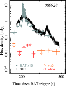
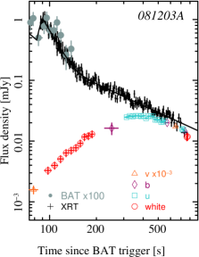
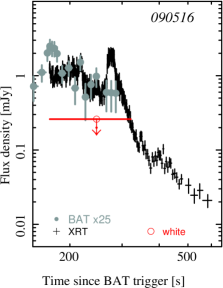
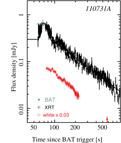
Figure 1.— Swift multi-wavelength light curves for the Gold Sample of X-ray flares. X-ray fluxes are corrected for Galactic and intrinsic absorption. UVOT fluxes have been renormalized to the V-band, and corrected for extinction.

UV/Optical Telescope (UVOT; Roming et al. 2005) photometric measurements were performed on a circular source extraction region with a radius of 5″. In case of faint ($\lesssim$0.5 cts s^-1) sources a 3″ radius aperture was used in order to optimize the signal-to-noise ratio and an aperture correction factor was applied for consistency with the UVOT calibration (Breeveld et al., 2010, 2011). The data were corrected for Galactic extinction (Schlegel et al., 1998) and, when possible, for intrinsic host extinction.

The Swift multi-wavelength light curves for the subsample of bursts with known redshift, which will be used for our broadband spectral modeling, are shown in Fig. 1.

2.3. Fermi/GBM data

We examined the daily Gamma-Ray Burst Monitor (GBM) CSPEC data searching for higher energy ($>$300 keV) counterparts of the X-ray flares. We considered the two GBM bismuth germanate (BGO) detectors and for the time of each flare selected the detector with the best view of the burst, i.e. with the smaller angle between the GRB’s direction and the detector. For each burst we examined the light curve in the 300 keV–10 MeV energy range. The expected number of background events (N_exp) was estimated by fitting a 2nd or 3rd order polynomial to the pre-flare and post-flare data, and by interpolating the fit during the X-ray flare time interval. The source significance was calculated as $\mathcal{S}=(\mathrm{N_{det}}-\mathrm{N_{exp}})/\sqrt{\mathrm{N_{exp}}}$, where N_det is the number of events detected during the flare time interval.

Only in the case of GRB 110102A, a significant detection (6.9$\,\sigma$) was found during the first flare. The signal is detected only up to 1 MeV, and is compatible with the extrapolation of the flare keV emission to higher energies. No significant increase of the event rate was visible in coincidence with any other X-ray flares.

By using a Bayesian approach with a flat prior $\pi(S)=1$ for $S>0$ and 0 otherwise on the signal S (Nakamura, 2010), we calculated an upper limit of confidence level CL on the number of signal events $S_{\mathrm{UL}}$ by numerically solving the following equation:

$$CL =\frac{\int^{S_{\mathrm{UL}}}_{-\infty}P_{G}(\mathrm{N_{det}},\mathrm{N_{exp}}+S)\pi(S)dS}{\int^{\infty}_{-\infty}P_{G}(\mathrm{N_{det}},\mathrm{N_{exp}}+S)\pi(S)dS}$$

$$=\frac{\int^{S_{\mathrm{UL}}}_{0}P_{G}(\mathrm{N_{det}},\mathrm{N_{exp}}+S)dS}{\int^{\infty}_{0}P_{G}(\mathrm{N_{det}},\mathrm{N_{exp}}+S)dS}$$ (1)

where $P_{G}(n,s)$ is the Poisson probability of detecting $s$ events when expecting $n$. We assumed no systematic uncertainties on the estimated number of background events N_exp. For each flare we generated the response matrix of the selected BGO detector by using GBM_RSP_Gen v. 1.8, and derived the detector effective area as a function of energy by assuming no energy-dispersion effects. A spectrally-weighted effective area, $A_{\mathrm{eff}}$, was calculated for a photon index $\Gamma$=2.0, and used to convert the upper limits into flux units. The derived values are listed in Table LABEL:gbmul. In the case of a spacecraft autonomous repointing (GRB 110731A, and GRB 110414A), the rapid change of the spacecraft’s orientation did not allow us to properly estimate the background level, and upper limits are not reported.

Table 2GBM Upper Limits

GRB	$t_{\rm i}$	$t_{\rm f}$	$F_{\rm 300keV-1\,MeV}$	$F_{\rm 1-10\,MeV}$
(1)	(2)	(3)	(4)	(5)
080906	160	240	2.4	2.3
	520	800	1.4	1.1
080928	340	400	5.2	4.4
081203A	98	154	3.8	4.5
090407	120	170	4.3	4.9
090516	260	315	6.0	4.9
090831C	160	260	3.4	3.7
091221	95	160	4.0	4.2
100725B	115	150	6.9	7.5
	150	200	5.7	6.3
	200	255	5.4	7.0
	255	315	5.1	5.7
100212A	76	85	10.3	11.3
	95	160	3.9	4.2
	223	243	7.0	7.6
	249	275	6.1	6.7
	344	383	5.1	5.5
	413	445	5.7	6.1
	628	750	3.1	3.3
110102A	249	393	–	4.7
	249	393	2.7	2.8

Notes : Col. (1): GRB name; Col. (2): start time of the search, in units of s; Col. (3): stop time of the search, in units of s; Col. (4): 95% upper limit in the 300 keV-1 MeV band. Units are 10^-2 ph cm^-2 s^-1. Col. (5): 95% upper limit in the 1 MeV-10 MeV band. Units are 10^-2 ph cm^-2 s^-1.

2.4. Fermi/LAT data

The LAT data were searched for emission related to the X-ray flares observed by Swift. We searched for emission coincident in time with each X-ray flare. In the case of a GRB afterglow with multiple flares, the search was also performed by stacking the data of the whole flaring activity, that is one search for the seven flares of GRB100212A, one for the four flares of GRB 100725B, one for the eight flares in GRB 100728A and one for the 2 flares of GRB 080906. According to some models, the high-energy emission could be delayed and longer-lasting than the lower energy flare. We therefore searched the LAT data for emission over longer time scales, performing our search over a period from the start time of the first flare and extending until the burst position exited the LAT FoV or became occulted by the Earth (up to 1 ks duration).

The searches were performed by means of an unbinned-likelihood analysis (Abdo et al., 2009). The searches over short time intervals ($<$400 s) were performed using the Pass 7 Transient Class (“P7TRANSIENT”) data, appropriate for signal-limited analyses, and the relevant instrument response function P7TRANSIENT_V6. The searches over longer-duration intervals were performed using the Pass 7 Source Class (“P7SOURCE”) data, appropriate for background-limited analyses, and the relevant instrument response function P7SOURCE_V6 (Ackermann et al., 2012).

The analysis used events reconstructed within 15^∘ around the XRT localization and with energies in the 100 MeV–10 GeV range. The X-ray flare spectrum was modeled using a power law with a free normalization and spectral index. The residual cosmic-ray background and the extragalactic gamma-ray background (CREGB) for the P7TRANSIENT analysis was estimated following the method described in Abdo et al. (2009); Vasileiou (2013). The Galactic diffuse background for both the P7TRANSIENT and P7SOURCE analyses, and the CREGB for the P7SOURCE analyses were modeled using the standard, publicly distributed, templates . The background contribution from the Earth’s atmospheric gamma-rays was negligible as the GRB positions were far from the Earth’s limb during all the time intervals analyzed. No point source in the vicinity of any of the analyzed GRBs (within 15^∘) was bright enough to merit inclusion in the background model. In the case of a stacked analysis, we simultaneously fit the likelihood functions of the flares under search. A single flux and spectral index were fit to the stacked data.

High-energy emission in coincidence with the observed X-ray flares was detected in the case of GRB 100728A, as reported in Abdo et al. (2011). For the other bursts in our sample we report in Table LABEL:latul the upper limits in the 100 MeV–10 GeV energy range. The quoted values are at a 95% confidence level, and were calculated for a photon index $\Gamma$=2.0. The upper limits calculation used a Bayesian approach with a flat prior, in which the profile likelihood was treated as the posterior probability of the source flux, as described in Section 2.3. The typical upper limit derived during each flare is an order of magnitude higher than the flux measured in the case of GRB 100728A. In the case of multiple flares, the upper limits derived from the stacked analysis are a few times higher. Two are the main differences between the flares in our sample and those in GRB 100728A: 1) GRB 100728A triggered an autonomuous repointing of the instrument, so that its emission during the flares was observed nearly on-axis where the sensitivity is maximum. All the flares in our sample were instead serendipitously observed by the LAT, mostly at large off-axis angles; 2) GRB 100728A displayed an unusual series of multiple, bright flares, and a detection was achieved only by considering the entire period of emission. Most bursts in our sample display instead one or two flares. Our results show that in general X-ray flares are not accompanied by a bright counterpart in the MeV-GeV energy range. The detection of a high-energy counterpart in GRB 100728A was the result of a fortunate combination of sensitive observations and long-lived flaring activity.

Table 3LAT Upper Limits

GRB	Description	$t_{\rm i}$	$t_{\rm f}$	$<$$F_{\gamma,UL}>$
(1)	(2)	(3)	(4)	(5)
080906	Flare #1	160	240	13
	Flare #2	520	800	4.2
	All Flares	–	–	3.3
	Extended Period	160	1160	1.7
080928	Flare	340	400	13
	Extended Period	340	1000	1.4
081203A	Flare	98	152	12
	Extended Period	98	1098	1.8
090407	Flare	120	170	15
	Extended Period	120	650	1.9
090516	Flare	260	315	30
	Extended Period	260	560	6.5
090831C	Flare	160	260	15
	Extended Period	160	1060	1.7
091221	Flare	95	160	15
	Extended Period	95	260	6.9
100212A	Flare #1	76	85	50
	Flare #2	95	160	23
	Flare #3	223	243	34
	Flare #4	249	275	40
	Flare #5	344	383	17
	Flare #6	413	445	21
	Flare #7	628	750	8.2
	All Flares	–	–	4.2
	Extended Period	76	976	1.4
100725B	Flare #1	115	150	17
	Flare #2	150	200	15
	Flare #3	200	255	9.9
	Flare #4	255	315	1.2
	All Flares	–	–	4.2
	Extended Period	115	1115	0.9
110102A	Flare #1	196	248	17
	Flare #2	249	393	4.5
	All Flares	–	–	3.5
	Extended Period	196	806	2.0
110414A	Flare	271	690	17
110731A	Flare	55	95	21

Notes : Col. (1): GRB name; Col. (2): We searched for high-energy emission in coincidence with each flare, by stacking the emission of multiple flares (All flares), and over longer timescales (Extended Period); Col. (3): start time of the search, in units of s; Col. (4): stop time of the search, in units of s; Col. (5): 95% upper limit in the 100 MeV-10 GeV band. Units are 10^-9 erg cm^-2 s^-1.

3. Theory and model description

We developed analytical prescriptions for the synchrotron, and first-order Inverse Compton components that include self-absorption, opacity for pair production and Thomson scattering on pairs, Klein-Nishina effects, and the maximum energy for acceleration. The model covers the various ordering of synchrotron self-absorption, maximum and cooling frequencies. The model was implemented for use within XSPEC for broadband spectral fitting. XSPEC allows for a simultaneous fit to all data sets by performing a minimization on the PG-STAT statistic on LAT data, and on $\chi^{2}$ on the data sets at lower energies. The use of PG-STAT is required by the low counts of LAT spectra, which are therefore Poissonian, and by the Gaussian uncertainties of the estimated LAT background (Vasileiou, 2013). In this case, neither the $\chi^{2}$ nor the Cash statistics yield accurate results (Arnaud et al., 2011). Spectra and response matrices for the Fermi data were created following Ackermann et al. (2013).

The spectrum produced by an ensemble of electrons accelerated by internal shocks is uniquely determined by six parameters (Sari et al., 1998; Piran, 2004), namely the internal energy of the shock $e^{\prime}$ (where primed quantities are in the rest frame of the shocked fluid), the fraction of energy that goes to electrons $\epsilon_{e}$ and to magnetic field $\epsilon_{B}$, the electron spectral index $p$, the bulk Lorentz factor $\Gamma$, and the radius of the source $R$. In the regime of fast cooling, which is the case relevant to our observations, it is more convenient to replace $e^{\prime}$ and $R$ with two related parameters more directly linked to observable quantities (Guetta & Granot, 2003). The first is the isotropic electron luminosity $L_{e}$=$\frac{4}{3}\pi R^{2}c\Gamma^{2}\epsilon_{e}e^{\prime}$ which is equal, for fast cooling, to the total (synchrotron plus higher IC orders) radiated luminosity $L_{\rm ISO}$=$L_{52}$10⁵² erg s^-1. The other is the variability time scale of the relativistic flow $t_{v}$, which in the internal shock model is related to the radius of the collision between shells by $R\approx 2\Gamma^{2}ct_{v}$.

Here we first briefly derive the characteristic frequencies of a synchrotron spectrum according to our formalism. Each electron radiates a power $P(\gamma)$ at a typical synchrotron frequency $\nu_{s}$:

$$P(\gamma)=\frac{4}{3}c\sigma_{T}\gamma^{2}\frac{B^{\prime 2}}{8\pi}\Gamma^{2}$$ (2)

$$\nu_{s}=\frac{3}{16}\frac{q_{e}B^{\prime}}{m_{e}c}\gamma^{2}\Gamma$$ (3)

where $B^{\prime}$ is the magnetic field, $\gamma$ the electron Lorentz factor, $m_{e}$ and $q_{e}$ its mass and electric charge respectively. The spectrum of the shock accelerated electrons is usually described as a power law with index $p$, $dn^{\prime}/d\gamma\propto\gamma^{-p}$ for $\gamma$$\geq$$\gamma_{m}$. We hardcoded a lower limit $p$$>2$ in the fitting routine in order to avoid divergent electron energies. The minimum Lorentz factor $\gamma_{m}$, and the corresponding frequency $\nu_{m}$ (from Eq. 3) are given by:

$$\gamma_{m} = \epsilon_{e}\frac{m_{p}}{m_{e}}\frac{p-2}{p-1}$$ (4a)

$$\nu_{m} = 2.6\times 10^{18}\ \left(\frac{p-2}{p-1}\right)^{2}\epsilon_{e}^{3/2}\epsilon_{B}^{1/2}L_{52}^{1/2}\Gamma_{2.5}^{-2}t_{v}^{-1}\ {\rm Hz\ \ \ \ \ \ \ }$$ (4b)

where $\Gamma_{2.5}=\Gamma/10^{2.5}$. The time scale for radiative cooling by synchrotron and IC becomes lower than the dynamical time scale above the cooling Lorentz factor $\gamma_{c}$ at the frequency $\nu_{c}$:

$$\gamma_{c} = 2(1+Y)^{-1}\epsilon_{e}\epsilon_{B}^{-1}L_{52}^{-1}\Gamma_{2.5}^{5}t_{v}$$ (5a)

$$\nu_{c} = 3.7\times 10^{12}(1+Y)^{-2}\epsilon_{e}^{3/2}\epsilon_{B}^{-3/2}L_{52}^{-3/2}\Gamma_{2.5}^{8}t_{v}{\rm Hz\ \ \ \ \ \ \ \ }$$ (5b)

where $Y$ is the Compton parameter. In the limit of single scattering, it can be approximated by the ratio of luminosities radiated by IC and synchrotron:

$$Y=\frac{L_{IC}}{L_{S}}=\frac{-1+\sqrt{1+4\eta\frac{\epsilon_{e}}{\epsilon_{B}}}}{2}$$ (6)

where the radiation efficiency $\eta\approx 1$ in the fast cooling regime. Likewise, the maximum Lorentz factor $\gamma_{M}$ of the electrons is derived by equating the acceleration time, which is essentially the Larmor time, with the dynamical time scale (Piran, 2004):

$$\gamma_{M} = 1.7\times 10^{6}(1+Y)^{-1/2}\epsilon_{e}^{1/4}\epsilon_{B}^{-1/4}L_{52}^{-1/4}\Gamma_{2.5}^{3/2}t_{v}^{1/2}$$ (7a)

$$\nu_{M} = 2.3\times 10^{24}(1+Y)^{-1}\Gamma_{2.5}{\rm Hz\ \ \ \ \ \ \ \ \ \ \ \ \ \ \ \ \ \ \ \ \ \ \ \ \ \ \ \ }$$ (7b)

where $\nu_{M}$ is the maximum synchrotron frequency.

We derived the spectrum for various ordering of the frequencies and extended the model prescriptions to the case of slow cooling. This has been necessary because the fitting procedure explores a wide range of parameters, often outside the region of fast cooling. Below we summarize the case $\nu_{c}<\nu_{sa}<\nu_{m}$ which applies to all the best-fit models. Specifically, in the fast cooling regime, the spectrum of electrons at equilibrium is given by:

$$N(\gamma)=N(\gamma_{c})\begin{cases}\left(\frac{\gamma}{\gamma_{c}}\right)^{-2}&\gamma_{c}<\gamma<\gamma_{m}\\ \left(\frac{\gamma}{\gamma_{c}}\right)^{-p-1}&\gamma_{m}<\gamma<\gamma_{M}\\ \end{cases}$$ (8)

where $p$ is the slope of the injection spectrum. Above $\nu>\nu_{\rm min}={\rm min}(\nu_{m},\nu_{c})$ the synchrotron spectrum can be derived by adopting the delta function approximation, i.e. assuming that all the power is radiated at the frequency given by Eq. 3. Then $L(\nu)d\nu=P(\gamma)N(\gamma)d\gamma$, using Eq. 2 and Eq. 8, yields:

$$L(\nu)=f_{\rm max}\left(\frac{\nu}{\nu_{c}}\right)^{-\frac{q-1}{2}}$$ (9)

where $q$=2 for $\gamma_{c}$$<$$\gamma$$<$$\gamma_{m}$ and $q$=$p+1$ for $\gamma_{m}$$<$$\gamma$$<$$\gamma_{M}$. The monochromatic luminosity $L_{\nu}$ peaks at $\nu_{c}$ and is $f_{\rm max}=m_{e}c^{2}\sigma_{T}\Gamma B^{\prime}N_{e}/6e$ where the total number of electrons $N_{e}=\gamma_{c}N(\gamma_{c})$ for $\gamma_{c}<<\gamma_{m}$.

At low frequencies the effect of synchrotron self-absorption becomes relevant. The absorption coefficient $\alpha_{\nu}$ can be specified (Panaitescu & Kumar, 2000) as:

$$\alpha_{\nu}\propto\begin{cases}\nu^{-5/3},&\mbox{for }\nu<\nu_{c}\\ \nu^{-3},&\mbox{for }\nu_{c}<\nu<\nu_{m}\end{cases}$$ (10)

and the spectrum can be derived recalling that, in the homogeneous case, the intensity in the optically thick regime is proportional to the source function (Rybicki & Lightman, 1979):

$$L_{\nu}\propto\frac{P(\nu)}{\alpha_{\nu}}\propto\begin{cases}\nu^{2},&\nu<\nu_{c}\\ \nu^{5/2},&\nu_{c}<\nu<\nu_{sa}\end{cases}$$ (11)

The synchrotron self absorption frequency $\nu_{sa}$ is derived by requiring that the optically thick emission (Eq. 11) equals the the optically thin emission (Eq. 9):

$$\nu_{sa}=9.2\times 10^{14}(1+Y)^{-1/3}\epsilon_{e}^{-1/3}L_{52}^{1/3}\Gamma_{2.5}^{-1}t_{v}^{-2/3}{\rm\ Hz\ \ \ \ }$$ (12)

Summarizing the above equations, the synchrotron spectrum is:

$$\frac{\nu L_{\nu}}{\nu_{m}L_{\nu_{m}}}=\begin{cases}\left(\frac{\nu_{sa}}{\nu_{m}}\right)^{1/2}\left(\frac{\nu_{c}}{\nu_{sa}}\right)^{7/2}\left(\frac{\nu}{\nu_{c}}\right)^{3},&\nu<\nu_{c}\\ \left(\frac{\nu_{sa}}{\nu_{m}}\right)^{1/2}\left(\frac{\nu}{\nu_{sa}}\right)^{7/2},&\nu_{c}<\nu<\nu_{sa}\\ \left(\frac{\nu}{\nu_{m}}\right)^{1/2},&\nu_{sa}<\nu<\nu_{m}\\ \left(\frac{\nu}{\nu_{m}}\right)^{1-p/2},&\nu_{m}<\nu<\nu_{M}\end{cases}$$ (13)

with the normalization

$$\nu_{m}L_{\nu_{m}}=5\times 10^{51}\left(\frac{p-2}{p-1}\right)(1+Y)^{-1}L_{52}\mbox{~{}erg\,s${}^{-1}$}$$ (14)

We also considered the case where the electron distribution is inhomogeneous (Granot et al., 2000). In this case a new absoption frequency $\nu_{ac}$$<$$\nu_{sa}$ appears. The spectrum is modified as $L_{\nu}$ $\propto$ $\nu^{11/8}$ for $\nu_{ac}$$<$$\nu<\nu_{sa}$, and $\L_{\nu}$ $\propto$ $\nu^{2}$ for $\nu$$<$$\nu_{ac}$ (Guetta & Granot, 2003).

The IC spectrum has been derived following the prescriptions of Sari & Esin (2001). In the Thomson limit, the energy of the upscattered photon is $\nu=4x\gamma^{2}\nu_{s}$, with $0<x\leq 1$ and the cross section is approximated by the Thompson value. The spectrum is then given by

$$L_{\nu}^{IC}=R\sigma_{T}\int_{\gamma_{min}}^{\infty}d\gamma N(\gamma)\int_{0}^{1}dx\ g(x)L_{\nu_{s}}(x)$$ (15)

where $\gamma_{\rm min}={\rm min}(\gamma_{c},\gamma_{m})$ and the Green function $g(x)$ (Blumenthal & Gould, 1970) gives the probability of producing an IC photon at frequency $\nu$ from a synchrotron photon at $\nu_{s}$. Following Sari & Esin (2001), we approximated $g(x)$$\sim$1 for $0<x<0.5$ The inner integral of Eq. 15 represents the IC spectrum produced by monoenergetic electrons. For a given power-law segment with $f(\nu_{s})\propto\nu_{s}^{\alpha}$, the integral becomes $I\propto\nu^{\alpha}$ for $\alpha<1$ and $I\propto\nu^{1}$ for $\alpha>1$. Thus the IC spectrum of monoenergetic electrons has the same shape above $\gamma^{2}\nu_{sa}$ as the input synchrotron spectrum above $\nu_{sa}$, with all frequencies boosted by a factor $\gamma^{2}$. Below $\gamma^{2}\nu_{sa}$ the effect of the distribution dominates and the integral is linear. For the case under examination (Eq. 13) the spectrum is:

$$I\propto f_{max}\begin{cases}\left(\frac{\nu_{sa}}{\nu_{c}}\right)^{-1/2}\left(\frac{\nu}{\gamma^{2}\nu_{sa}}\right),&\nu<\gamma^{2}\nu_{sa}\\ \left(\frac{\nu_{m}}{\nu_{c}}\right)^{-1/2}\left(\frac{\nu}{\gamma^{2}\nu_{m}}\right)^{-1/2},&\gamma^{2}\nu_{sa}<\nu<\gamma^{2}\nu_{m}\\ \left(\frac{\nu_{m}}{\nu_{c}}\right)^{-1/2}\left(\frac{\nu}{\gamma^{2}\nu_{m}}\right)^{-p/2},&\gamma^{2}\nu_{m}<\nu\\ \end{cases}$$ (16)

Note that the shape of the IC spectrum below $\gamma^{2}\nu_{sa}$ is the same for either the homogenous and inhomogeneous cases because below $\nu_{sa}$ the corresponding power-law segments have indices greater than 1. Substituting Eq. 16 in Eq. 15 gives the approximate solution:

$$\nu L^{IC}_{\nu}\approx\nu_{m}^{IC}L_{\nu_{m}}^{IC}\begin{cases}\left(\frac{\nu_{sa}^{IC}}{\nu_{m}^{IC}}\right)^{1/2}\left(\frac{\nu}{\nu_{sa}^{IC}}\right)^{2},&\nu<\nu_{sa}^{IC}\\ \left(\frac{\nu}{\nu_{m}^{IC}}\right)^{1/2},&\nu_{sa}^{IC}<\nu<\nu_{m}^{IC}\\ \left(\frac{\nu}{\nu_{m}^{IC}}\right)^{1-p/2},&\nu_{m}^{IC}<\nu<\nu_{M}^{IC}\\ \end{cases}$$ (17)

where

$$\nu_{m}^{IC}L_{\nu_{m}}^{IC} = Y\nu_{m}L_{\nu_{m}}$$

$$\nu_{sa}^{IC} = \gamma^{2}_{c}\nu_{sa}$$

$$\nu_{m}^{IC} = \gamma_{m}^{2}\nu_{m}$$

$$\nu_{M}^{IC} = \gamma_{M}^{2}\nu_{M}$$ (18)

and the corresponding numerical values are obtained by substituting Eq. 4b, 5a, 7a, 12, 14. The spectral shape given in Eq. 21 was derived by assuming the IC scattering to take place in the Thomson regime, i.e., when the $\gamma h\nu_{s}<\Gamma mc^{2}$. Electrons with $\gamma>\tilde{\gamma}_{m}=\frac{mc^{2}\Gamma}{h\nu_{m}}$ interact with photons with $\nu>\nu_{m}$ in the Klein-Nishina regime. In this regime, the upscattered energy is $h\nu^{IC}=\Gamma\gamma mc^{2}$. Thus the transition appears in the IC spectrum at:

$$h\nu_{KN}^{IC}=\tilde{\gamma}_{m}mc^{2}\Gamma=\frac{(mc^{2})^{2}\Gamma^{2}}{h\nu_{m}}\\$$ (19)

when $\nu_{KN}^{IC}<\nu_{M}^{IC}$ with

$$\nu_{M}^{IC}=\frac{\gamma_{M}mc^{2}}{h}\Gamma$$ (20)

In this energy range, the spectrum can be approximated by $L_{\nu}^{IC}\propto\nu^{-(p+1)/2}$ (Guetta & Granot, 2003). Nakar et al. (2009) presented a more detailed calculation of the Klein-Nishina regime, showing that the spectral shape could be significantly modified with respect to the simple treatment of Guetta & Granot (2003). However, as in our case the peak of the synchrotron emission is in the soft X-ray range, Klein-Nishina effects can be considered negligible, and the adopted approximation does not affect our results. In fact, in fast cooling, the Klein-Nishina effects can be neglected when $\gamma_{m}<<{~{}\tilde{\gamma}}_{m}$. By substituting Eq. 4b, we derive the condition $\Gamma>>\epsilon_{e}\frac{h\nu_{m}}{1\rm keV}$, which is always satisfied for the kind of relativistic flow that we consider here.

In the low energy part of the spectrum, the IC photons are also subject to synchrotron absorption at $\nu$$<$$\nu_{sa}$, when the source becomes optically thick. In this regime, the spectrum is proportional to the source function (Eq. 11) which, for the absorption coefficient given in Eq. 10, yields $L_{\nu}^{IC}\propto\nu^{4}$. The overall IC spectrum is then:

$$\frac{\nu L^{IC}_{\nu}}{\nu_{m}^{IC}L_{\nu_{m}}^{IC}}=\begin{cases}\left(\frac{\nu_{sa}^{IC}}{\nu_{m}^{IC}}\right)^{1/2}\left(\frac{\nu_{sa}}{\nu_{sa}^{IC}}\right)^{2}\left(\frac{\nu}{\nu_{sa}}\right)^{5},&\nu<\nu_{sa}\\ \left(\frac{\nu_{sa}^{IC}}{\nu_{m}^{IC}}\right)^{1/2}\left(\frac{\nu}{\nu_{sa}^{IC}}\right)^{2},&\nu_{sa}<\nu<\nu_{sa}^{IC}\\ \left(\frac{\nu}{\nu_{m}^{IC}}\right)^{1/2},&\nu_{sa}^{IC}<\nu<\nu_{m}^{IC}\\ \left(\frac{\nu}{\nu_{m}^{IC}}\right)^{1-p/2},&\nu_{m}^{IC}<\nu<\nu_{KN}^{IC}\\ \left(\frac{\nu_{IC}^{KN}}{\nu_{m}^{IC}}\right)^{1-p/2}\left(\frac{\nu}{\nu_{KN}^{IC}}\right)^{1/2-p},&\nu_{KN}^{IC}<\nu<\nu_{M}^{IC}\end{cases}$$ (21)

In the high energy part of the spectrum, photons with energy $h\nu_{\gamma\gamma}$ can interact with photons at energies $h\nu_{an}$ $\geq$ ${(\Gamma mc^{2})^{2}}/{h\nu_{\gamma\gamma}}$ and annihilate in pairs. In the case under study, by requiring that the optical depth for pair production $\tau_{\gamma\gamma}$ is less than unity (Lithwick & Sari, 2001) one obtains a spectral cut-off at:

$$\nu_{\gamma\gamma}=5.6\times 10^{25}(1+Y)^{\frac{2}{p}}(\epsilon_{e}^{3}\epsilon_{B})^{\frac{2-p}{2p}}L_{52}^{(\frac{p+2}{2p})}t_{v}\Gamma_{2.5}^{\frac{4(p+1)}{p}}{\rm Hz}$$ (22)

Finally, the optical depth for Thomson scattering on the pairs has to be smaller than one. Taking into account that the number of pairs is equal to the number of photons that annihilate, this condition is satisfied when the cut-off energy for pair production in the rest frame of the shell is greater than $mc^{2}$ (e.g. Abdo et al., 2009). By implementing the prescriptions of Lithwick & Sari (2001) we derive $\frac{h\nu_{\gamma\gamma}}{\Gamma}\gtrsim 3mc^{2}$, which gives a lower limit on the bulk Lorentz factor $\Gamma$:

$$\Gamma\gtrsim 220(1+Y)^{\frac{-2}{3p+4}}(\epsilon_{e}^{3}\epsilon_{B})^{\frac{p-2}{2(3p+4)}}L_{52}^{\frac{p+2}{2(3p+4)}}t_{v,-2}^{\frac{-p}{3p+4}}$$ (23)

Equations (22, 23) apply to the case in which high energy photons annihilate on target photons dominated by the synchrotron component, that is the most common situation. In the IC case the cut-off energy can be significantly lower, modifying Eq. 22 by a factor $Y^{-\frac{2}{p}}\gamma_{m}^{-\frac{2(p-2)}{p}}$. This is taken into account in the fitting program by implementing, in addition to the analytical approach, an iterative routine to avoid the regions of parameter space that do not satisfy the opacity constraints.

It is useful for the discussion below to rewrite the condition for Thomson opacity on pairs as an upper limit to $t_{v}$ in terms of two observable quantities, $\nu_{m}$ and the flux $F_{\nu_{m}}$:

$$t_{v}\lesssim 0.2{\rm\ }\left(1+Y\right)^{\frac{p+8}{2(p+4)}}\left(\epsilon_{e,-1}^{3}\epsilon_{B,-1}\right)^{\frac{p+8}{2(p+4)}}\left(\frac{h\nu_{m}}{{\rm 1\,keV}}\right)^{-\frac{3p+4}{p+4}}$$

$$t_{v}\lesssim \left(\frac{\nu_{m}F_{\nu_{m}}}{10^{-9}~{}{\rm erg\,cm^{-2}\,s^{-1}}}\right)^{\frac{p}{2(p+4)}}D_{28}^{\frac{p}{p+4}}$$ (24a)

$$t_{v}\lesssim$$

$$t_{v}\lesssim$$

$$t_{v}\lesssim 0.08{\rm\ }\left(\frac{Y}{10}\right)^{\frac{p}{2(p+4)}}\epsilon_{e,-1}^{\frac{5(8-p)}{2(p+4)}}\epsilon_{B,-1}^{\frac{(8+p)}{2(p+4)}}\left(\frac{h\nu_{m}}{{\rm keV}}\right)^{-\frac{3p+4}{p+4}}$$

$$t_{v}\lesssim \left(\frac{\nu_{m}F_{\nu_{m}}}{10^{-9}~{}{\rm erg\,cm^{-2}\,s^{-1}}}\right)^{\frac{p}{2(p+4)}}D_{28}^{\frac{p}{p+4}}$$ (24b)

Equation 24a applies when the opacity is dominated by synchrotron. When the $Y$-parameter increases, the opacity is more likely dominated by target photons on the IC component (Eq. 24b). The numerical factor is computed for $p$=2.5 and varies by less than 30% for 2.5$<$$p$$<$3.

4. Results

4.1. Constraints on IC processes

Before presenting the results of the broadband fits, we discuss some general properties of the flares and their implications. As reported in Table 1, X-ray flares are characterized by a peak energy within or below the X-ray band, a typical flux $f_{X}\approx 10^{-9}-10^{-8}$ erg cm^-2 s^-1, and an observed duration $\Delta t$$\approx$10-100 s. In agreement with previous studies on X-ray flares (Falcone et al., 2007), we found that $\sim$40% of the spectra are curved and can be described by a Band function with $\alpha$$\approx$1.0 and $\beta$$\approx$2.4, and a peak energy of a few keV. In the remaining cases a power law with photon index $\Gamma$$\approx$2.2 is already a good fit, suggesting that the spectral peak is below the XRT energy band.

A common feature of the flares in our sample is that usually no bright optical counterpart is observed during the time interval of the X-ray flares, despite the good and simultaneous sampling with the UVOT (see Figure 1). The optical afterglow, when detected, does not show in general significant variability, suggesting that emission from the forward shock is likely the dominant component. The optical counterpart of X-ray flares remains hidden within the measurement uncertainty, which we adopt as an upper limit to the optical flare emission.

For a typical X-ray flux $\gtrsim$10^-9 erg cm^-2 s^-1, the optical non-detection implies an optical-to-X-ray spectral index $\beta_{ox}<0.5$. Such a flat spectrum could be due to a significant absorption affecting the UV-optical range. However it is unlikely that external factors (dusty environment, or high redshift) contribute to the suppression of optical emission in the whole sample, and they can be ruled out for those GRBs with a measured redshift and intrinsic extinction. The absence of optical flares is more likely an intrinsic property of the spectra of the X-ray flares, which could be explained either if the synchrotron self-absorption frequency $\nu_{sa}$ is above the optical band, or if the X-ray flare is produced by the IC scattering of optical/infrared synchrotron photons (Kobayashi et al., 2007). In the latter case, the lack of an optical counterpart implies that the low-energy synchrotron component is suppressed by an efficient ($Y$$>>$1) IC cooling, and therefore a bright second-order IC component, peaking at $\nu_{\gamma}$$\approx$10-100 MeV, should be visible. The simultaneous Fermi-GBM and Fermi-LAT observations disfavor this scenario, as we discuss below. The X-ray-to-optical flux ratio can be used to set a lower limit on the $Y$ parameter, derived by combining Equations 13, and 18:

$$Y\gtrsim\left(\frac{\nu_{X}f_{X}}{\nu_{opt}f_{opt}}\right)\left(\frac{\nu_{opt}\nu_{\gamma}}{\nu_{X}^{2}}\right)^{1+\beta}$$ (25)

where $\nu_{\gamma}$ is the peak frequency of the second-order IC component. The second term in Equation 25 takes into account the fact that the synchrotron peak lies below the observed optical range, at a frequency $\nu_{m}$$\approx$$\nu_{X}^{2}/\nu_{\gamma}$.

As $\nu_{\gamma}$ lies either in the GBM or LAT energy band, the gamma-ray-to-X-ray flux ratio sets an upper limit on the $Y$ parameter: $Y\lesssim f_{\gamma}\nu_{\gamma}/f_{X}\nu_{X}$. Such a limit is valid in the case of optically thin emission, which for a mildly relativistic outflow, $\Gamma$$\gtrsim$5 (1+$z$), is always satisfied at an energy of $\approx$10 MeV.

As shown in Fig. 2, the constraints derived from optical and gamma-ray observations are inconsistent for the bright flares ($f_{X}$$>$10^-8 erg cm^-2 s^-1) in our sample: the lower limits derived from optical data require in most cases $Y$$>$100, while the upper limits derived from gamma-ray data [GBM (top panel), and LAT (bottom panel)] imply much lower values of the $Y$-parameter, not consistent with the constraints derived from optical data. Therefore, the X-ray emission is unlikely to be dominated by the IC component.

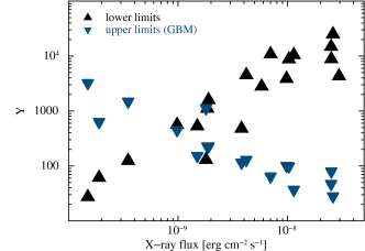
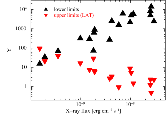
Figure 2.— Top panel: Constraints on the Y-parameter as a function of the observed X-ray flux. The lower limits on the $Y$-parameter were calculated according to Eq. 25 for an IC peak frequency $\nu_{\gamma}$=10 MeV. Upper limits were derived from Fermi/GBM observations. Bottom panel: Constraints to the Y-parameter as a function of the observed X-ray flux. The lower limits on the $Y$-parameter were calculated according to Eq. 25 for an IC peak frequency $\nu_{\gamma}$=100 MeV. Upper limits were derived from Fermi/LAT observations.

4.2. Broadband spectral modeling

Table 4Results of the broadband fit

GRB	$L_{52}$	$\epsilon_{e}$	$\epsilon_{B}$	$p$	$t_{v}$	$\Gamma$	${\rm STAT/dof}$
(1)	(2)	(3)	(4)	(5)	(6)	(7)	(8)
080906	$0.05\pm 0.02$	$0.35^{+0.10}_{-0.3}$	$0.45^{+0.10}_{-0.15}$	2.1$\pm$0.1	0.1 s	76$\pm$10	113/94
	$0.11^{+0.12}_{-0.06}$	0.43${}^{+0.10}_{-0.4}$	0.07${}^{+0.4}_{-0.05}$	2.1$\pm$0.1	1 ms	270${}^{+130}_{-50}$	74/94
080928	$0.012_{-0.002}^{+0.002}$	$0.30_{-0.07}^{+0.10}$	$0.60_{-0.10}^{+0.10}$	2.68${}^{+0.10}_{-0.18}$	0.1 s	$56_{-6}^{+10}$	163/127
	$0.020^{+0.05}_{-0.005}$	$>0.08$	$>0.01$	$2.4^{+0.4}_{-0.2}$	1 ms	$400_{-200}^{+150}$	164/127
081203A	0.21${}^{+0.17}_{-0.10}$	0.26${}^{+0.12}_{-0.05}$	1.4${}^{+2.3}_{-0.9}$$\times$10-2	2.23${}^{+0.3}_{-0.10}$	1 ms	300${}^{+40}_{-50}$	363/229
090516	$0.26^{+0.12}_{-0.02}$	$0.21_{-0.03}^{+0.12}$	$>0.25$	$3.2^{+0.3}_{-0.4}$	0.1 s	$100^{+25}_{-5}$	157/157
	$0.5_{-0.3}^{+0.5}$	$>0.02$	$>0.03$	$3.2_{-0.4}^{+0.3}$	1 ms	$>280$	159/157
110731A	$0.43^{+0.16}_{-0.18}$	$0.44_{-0.3}^{+0.11}$	$0.19_{-0.09}^{+0.11}$	$2.08^{+0.04}_{-0.07}$	0.1 s	115$\pm$15	120/104
	$0.33_{-0.18}^{+0.2}$	$0.46_{-0.26}^{+0.04}$	$0.16_{-0.08}^{+0.16}$	2.13$\pm$0.12	1 ms	$450_{-200}^{+300}$	104/104

Notes : Col. (1): GRB name; Col. (2): Bolometric luminosity (units are 10⁵² erg cm^-2 s^-1); Col. (3): electron energy fraction; Col. (4): magnetic energy fraction; Col. (5): electrons spectral index; Col. (6): variability timescale; Col. (7): Lorentz factor; Col. (8): best fit statistic;

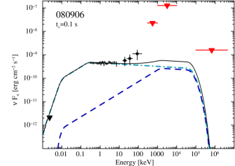
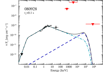
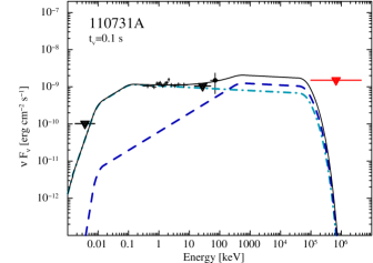
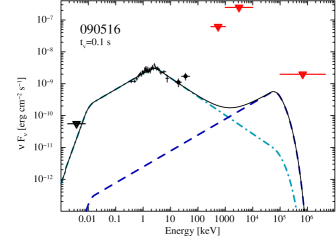
Figure 3.— Broadband spectra of X-ray flares comparing Swift (black) and Fermi (red) data with the standard internal shock model. The best-fit model for $t_{v}$=0.1 s is shown by the solid line. The synchrotron component is shown by the dot-dashed line, the IC component by the dashed line. The LAT upper limits were calculated in two energy bands, 100 MeV - 3 GeV and 3 GeV - 30 GeV, using the procedure described in Section. 2.4, and converted into energy flux units using the best-fit spectral model. Upper limits above 3 GeV are out of scale, and are not shown.

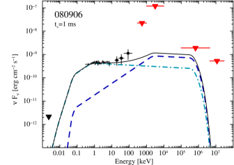
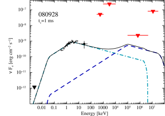
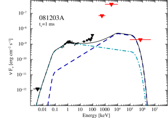
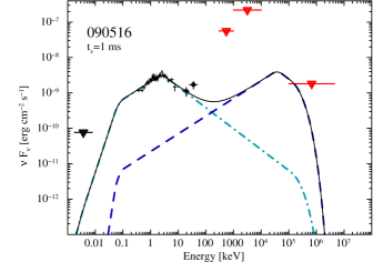
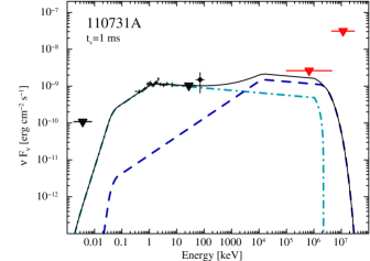
Figure 4.— Broadband spectra of X-ray flares comparing Swift (black) and Fermi (red) data with the standard IS model. The best fit model for $t_{v}$=1 ms is shown by the solid line. The synchrotron component is shown by the dot-dashed line, the IC component by the dashed line. The LAT upper limits were calculated in two energy bands, 100 MeV - 3 GeV and 3 GeV - 30 GeV, using the procedure described in Section. 2.4, and converted into energy flux units using the best fit spectral model. In the case of GRB 081203A and 090516, upper limits above 3 GeV are out of scale, and are not shown.

Now we turn to the detailed description of spectral modelling of the bursts with known redshift. The lack of a high-energy counterpart removes a relevant constraint to the model. In order to limit the number of free parameters we performed the spectral fits by fixing the variability timescales to three different values, $t_{v}$=$\Delta t/(1+z)$, that is the flare duration, $t_{v}$=0.1 s, and $t_{v}$=1 ms, similar to the variability timescale of the prompt emission. The former choice did not provide any acceptable fit unless we introduced a substantial extinction ($A_{V}>>1$). This is because, within the internal shock scenario, a long variability timescale would predict a low self-absorption frequency and therefore an optical flux much larger than the measured values. This can be consistent with the observations only if a significant amount of dust suppresses the optical emission. As no afterglow in our sample shows evidence of such a feature, the absorber should be closer to the central source, where dust cannot survive the strong photon flux produced by the GRB. Therefore, within the internal shock scenario, we found that the condition $t_{v}$$\approx$$\Delta t$ cannot reproduce the observed data. This result can be understood by examining in more detail how the constraints on the optical and gamma-ray fluxes relate to the variability time scale $t_{v}$. Equation (24a) allows us to derive an upper limit $t_{v}\lesssim 0.2$  $(h\nu_{m}/1~{}{\rm keV})^{-7/4}$ s, that applies if the X-ray flare emission is dominated by the synchrotron component. If the flare duration represents its typical variability timescale, the Thomson opacity constraint requires $h\nu_{m}\ll 1$ kev. Thus, assuming that the X-ray emission is dominated by the synchrotron tail at $\nu\gg\nu_{m}$, the flux at lower energies would increase with decreasing energy down to $\nu_{sa}$. For large values of $t_{v}$, $\nu_{sa}$ (Equation 12) is much lower than the X-ray range, and the flux predicted in the optical band would violate the observed upper limits. If no substantial extinction is present, $\nu_{sa}$ has to be large in order not to overcome the optical limits. This condition implies again small values of $t_{v}\ll\Delta t$. The assumption that the flare duration reflects the typical timescale of the relativistic outflow holds if the X-ray flare emission is mostly produced by IC processes. As discussed in the previous section, this is in constrast with the Fermi observations.

In Table 4 we report the best fit results for the shorter timescales, $t_{v}=0.1$ s and $t_{v}=1$ ms. Based on our dataset we cannot discriminate between these two values, and both fits represent an acceptable description of the data. The broadband spectra and best-fit models are shown in Fig. 3, and in Fig. 4, respectively. The cases of GRB 080906 and GRB 110731A are the least constrained, as only a simple power-law component is present in the X-ray spectrum (see Tab. 1). In the cases of GRB 080928 and GRB 090516 the peak of the synchrotron component lies in the XRT band, allowing for better constraints on the parameters. Above the peak, the photon indices are $\Gamma$=$p/2+1$$\sim$2.1 and 2.6, respectively, consistent with the phenomenogical fits of Tab. 1. The derived Lorentz factors range between 50 and 120 for $t_{v}$=0.1 s, corresponding to a radius $R$$\approx$10¹³-10¹⁴ cm, in agreement with the late internal shock scenario (Fan & Wei, 2005). Larger Lorentz factors are required for $t_{v}$=1 ms, ranging from 200 to 1000, which correspond to $R$$\approx$2$\times$10¹²-6$\times$10¹³ cm. As a comparison, a Lorentz factor $\Gamma$$\sim$300-550 was derived for the prompt gamma-ray emission phase of GRB 110731A (Ackermann et al., 2013). Independent on the value of $t_{v}$, we found 0.1 $\lesssim$ $\epsilon_{B}/\epsilon_{e}$ $\lesssim$ 1, and therefore no bright SSC component is expected at high energies. The typical Fermi GBM upper limit does not exclude the presence of a MeV counterpart 100 times brighter than the observed X-ray flare. However, the emergence of such a component would also affect the BAT spectrum, which, thanks to the sensitivity of the Swift/BAT, provides a tight constraint on the models.

GRB 081203A is the only case characterized by a turn up in the BAT spectrum, modeled as the rise of the SSC emission. Contrary to the other cases, a small value of the magnetic field, $\epsilon_{B}$$\approx$10^-2, and a larger value of $Y\gg 1$ are needed to account for the observed hard X-ray emission. As $h\nu_{m}$$\approx$1 keV, the opacity requirement (Eq. 24b) yields $t_{v,{\rm max}}$ $\propto$ 0.08 $Y^{-4/(p+4)}$ s, and favors the shortest variability timescales. In fact, for this flare no acceptable fit was found for $t_{v}$=0.1 s, and a variability timescale as short as 1 ms provided a better description. This result holds if the emission above 15 keV is associated to the flare. A different possibility is that the underlying afterglow, subdominant in the soft X-ray band, becomes visible in the BAT energy range. In the latter hypothesis, no bright SSC flare component is required, and the properties of this X-ray flare are analoguous to rest of the sample.

5. Conclusion

We presented a systematic search for high-energy emission associated with X-ray flares. We found that in general X-ray flares are not accompanied by a bright counterpart in the MeV-GeV energy range. By assuming a flat power-law energy spectrum, we derived typical upper limits of 10^-7 erg cm^-2 s in the 1 MeV-10 MeV energy band, and 10^-8 erg cm^-2 s in the 100 MeV-10 GeV band. Interestingly, no bright optical counterpart is observed during the periods of flaring activity. The lack of optical and gamma-ray detections disfavors IC processes as the main radiation mechanism producing the observed X-ray emission.

For bursts with a measured redshift, we carried out a more detailed analysis in the context of the internal shock model. This model is a good fit for all the flares and is consistent with the canonical scenario where the relativistic ($\Gamma>50$) outflow first undergoes internal shocks at a radius $\approx$10¹³-10¹⁴ cm and then, at larger radii, external shocks. X-ray flares carry a substantial fraction of the radiated energy, ranging from $\approx 10^{51}$ erg to $\approx 10^{53}$ erg (isotropic equivalent), that is from 6% to 100% of the energy observed during the prompt gamma-ray phase.

Particularly compelling are the implications on the variability timescale, which in all cases was significantly shorter than the flare duration. The broadband data are not consistent with the simplest scenario, in which the flare is caused by a “single event”, produced by the interaction of two shells colliding at a radius $\approx 2\Gamma^{2}c\Delta t$. The flare light curve reflects instead the profile of the relativistic outflow, modulated by the central engine on a timescale $t_{v}\lesssim 0.1$ s. Longer time scales for variability would be allowed if the synchrotron emissio peaked significantly below the X-ray band, but this condition is not consistent with the optical and gamma-ray upper limits. Within the internal shock model considered here, the duration of the X-ray flare is mainly set by the prolonged activity of the inner engine. This is a strong requirement for GRB central engines, as the observed durations of X-ray flares are often comparable or even exceed the durations of the prompt gamma-ray phases.

References

- Abdo et al. (2011) Abdo, A. A., Ackermann, M., Ajello, M., et al. 2011, ApJ, 734, L27+
- Abdo et al. (2009) Abdo, A. A., Ackermann, M., Asano, K., et al. 2009, ApJ, 707, 580
- Ackermann et al. (2012) Ackermann, M., Ajello, M., Albert, A., et al. 2012, ApJS, 203, 4
- Ackermann et al. (2013) Ackermann, M., Ajello, M., Asano, K., et al. 2013, ApJ, 763, 71
- Ackermann et al. (2013) Ackermann et al. 2013, ApJS, 209, 11
- Arnaud et al. (2011) Arnaud, K., Smith, R., & Siemiginowska, A. 2011, Handbook of X-ray Astronomy, ed. R. Ellis, J. Huchra, S. Kahn, G. Rieke, & P. B. Stetson
- Arnaud (1996) Arnaud, K. A. 1996, in Astronomical Society of the Pacific Conference Series, Vol. 101, Astronomical Data Analysis Software and Systems V, ed. G. H. Jacoby & J. Barnes, 17–+
- Atwood et al. (2009) Atwood, W. B., Abdo, A. A., Ackermann, M., et al. 2009, ApJ, 697, 1071
- Band et al. (1993) Band, D., Matteson, J., Ford, L., et al. 1993, ApJ, 413, 281
- Baring & Harding (1997) Baring, M. G. & Harding, A. K. 1997, ApJ, 491, 663
- Barthelmy et al. (2005a) Barthelmy, S. D., Barbier, L. M., Cummings, J. R., et al. 2005a, Space Sci. Rev., 120, 143
- Barthelmy et al. (2005b) Barthelmy, S. D., Chincarini, G., Burrows, D. N., et al. 2005b, Nature, 438, 994
- Beloborodov et al. (2011) Beloborodov, A. M., Daigne, F., Mochkovitch, R., & Uhm, Z. L. 2011, MNRAS, 410, 2422
- Blumenthal & Gould (1970) Blumenthal, G. R. & Gould, R. J. 1970, Reviews of Modern Physics, 42, 237
- Breeveld et al. (2010) Breeveld, A. A., Curran, P. A., Hoversten, E. A., et al. 2010, MNRAS, 406, 1687
- Breeveld et al. (2011) Breeveld, A. A., Landsman, W., Holland, S. T., et al. 2011, in American Institute of Physics Conference Series, Vol. 1358, American Institute of Physics Conference Series, ed. J. E. McEnery, J. L. Racusin, & N. Gehrels, 373–376
- Burrows et al. (2005a) Burrows, D. N., Hill, J. E., Nousek, J. A., et al. 2005a, Space Sci. Rev., 120, 165
- Burrows et al. (2005b) Burrows, D. N., Romano, P., Falcone, A., et al. 2005b, Science, 309, 1833
- Chincarini et al. (2007) Chincarini, G., Moretti, A., Romano, P., et al. 2007, ApJ, 671, 1903
- Curran et al. (2008) Curran, P. A., Starling, R. L. C., O’Brien, P. T., et al. 2008, A&A, 487, 533
- Evans et al. (2009) Evans, P. A., Beardmore, A. P., Page, K. L., et al. 2009, MNRAS, 397, 1177
- Evans et al. (2007) Evans, P. A., Beardmore, A. P., Page, K. L., et al. 2007, A&A, 469, 379
- Falcone et al. (2006) Falcone, A. D., Burrows, D. N., Lazzati, D., et al. 2006, ApJ, 641, 1010
- Falcone et al. (2007) Falcone, A. D., Morris, D., Racusin, J., et al. 2007, ApJ, 671, 1921
- Fan et al. (2008) Fan, Y.-Z., Piran, T., Narayan, R., & Wei, D.-M. 2008, MNRAS, 384, 1483
- Fan & Wei (2005) Fan, Y. Z. & Wei, D. M. 2005, MNRAS, 364, L42
- Fryer & Mészáros (2003) Fryer, C. L. & Mészáros, P. 2003, ApJ, 588, L25
- Galli & Piro (2006) Galli, A. & Piro, L. 2006, A&A, 455, 413
- Galli & Piro (2007) Galli, A. & Piro, L. 2007, A&A, 475, 421
- Gehrels et al. (2004) Gehrels, N., Chincarini, G., Giommi, P., et al. 2004, ApJ, 611, 1005
- Giannios (2006) Giannios, D. 2006, A&A, 455, L5
- Goad et al. (2007) Goad, M. R., Page, K. L., Godet, O., et al. 2007, A&A, 468, 103
- Granot et al. (2000) Granot, J., Piran, T., & Sari, R. 2000, ApJ, 534, L163
- Guetta et al. (2007) Guetta, D., Fiore, F., D’Elia, V., et al. 2007, A&A, 461, 95
- Guetta & Granot (2003) Guetta, D. & Granot, J. 2003, ApJ, 585, 885
- He et al. (2012) He, H.-N., Zhang, B.-B., Wang, X.-Y., Li, Z., & Mészáros, P. 2012, ApJ, 753, 178
- Ioka et al. (2005) Ioka, K., Kobayashi, S., & Zhang, B. 2005, ApJ, 631, 429
- Jakobsson et al. (2004) Jakobsson, P., Hjorth, J., Fynbo, J. P. U., et al. 2004, ApJ, 617, L21
- Kalberla et al. (2005) Kalberla, P. M. W., Burton, W. B., Hartmann, D., et al. 2005, A&A, 440, 775
- King et al. (2005) King, A., O’Brien, P. T., Goad, M. R., et al. 2005, ApJ, 630, L113
- Kobayashi et al. (2007) Kobayashi, S., Zhang, B., Mészáros, P., & Burrows, D. 2007, ApJ, 655, 391
- Krimm et al. (2007) Krimm, H. A., Granot, J., Marshall, F. E., et al. 2007, ApJ, 665, 554
- La Parola et al. (2006) La Parola, V., Mangano, V., Zhang, B., et al. 2006, Nuovo Cimento B Serie, 121, 1505
- Lazzati et al. (2011) Lazzati, D., Blackwell, C. H., Morsony, B. J., & Begelman, M. C. 2011, MNRAS, 411, L16
- Lazzati & Perna (2007) Lazzati, D. & Perna, R. 2007, MNRAS, 375, L46
- Liang et al. (2006) Liang, E. W., Zhang, B., O’Brien, P. T., et al. 2006, ApJ, 646, 351
- Lithwick & Sari (2001) Lithwick, Y. & Sari, R. 2001, ApJ, 555, 540
- Lü & Zhang (2014) Lü, H.-J. & Zhang, B. 2014, ApJ, 785, 74
- Lyons et al. (2010) Lyons, N., O’Brien, P. T., Zhang, B., et al. 2010, MNRAS, 402, 705
- Maxham & Zhang (2009) Maxham, A. & Zhang, B. 2009, ApJ, 707, 1623
- Melandri et al. (2012) Melandri, A., Sbarufatti, B., D’Avanzo, P., et al. 2012, MNRAS, 421, 1265
- Mesler et al. (2012) Mesler, R. A., Whalen, D. J., Lloyd-Ronning, N. M., Fryer, C. L., & Pihlström, Y. M. 2012, ApJ, 757, 117
- Nakamura (2010) Nakamura, K. 2010, Journal of Physics G Nuclear Physics, 37, 075021
- Nakar et al. (2009) Nakar, E., Ando, S., & Sari, R. 2009, ApJ, 703, 675
- Nousek et al. (2006) Nousek, J. A., Kouveliotou, C., Grupe, D., et al. 2006, ApJ, 642, 389
- O’Brien et al. (2006) O’Brien, P. T., Willingale, R., Osborne, J., et al. 2006, ApJ, 647, 1213
- Page et al. (2007) Page, K. L., Willingale, R., Osborne, J. P., et al. 2007, ApJ, 663, 1125
- Panaitescu (2008) Panaitescu, A. 2008, MNRAS, 383, 1143
- Panaitescu & Kumar (2000) Panaitescu, A. & Kumar, P. 2000, ApJ, 543, 66
- Perna et al. (2006) Perna, R., Armitage, P. J., & Zhang, B. 2006, ApJ, 636, L29
- Perri et al. (2007) Perri, M., Guetta, D., Antonelli, L. A., et al. 2007, A&A, 471, 83
- Piran (2004) Piran, T. 2004, Reviews of Modern Physics, 76, 1143
- Piro et al. (1998) Piro, L., Amati, L., Antonelli, L. A., et al. 1998, A&A, 331, L41
- Piro et al. (2005) Piro, L., De Pasquale, M., Soffitta, P., et al. 2005, ApJ, 623, 314
- Proga & Zhang (2006) Proga, D. & Zhang, B. 2006, MNRAS, 370, L61
- Roming et al. (2005) Roming, P. W. A., Kennedy, T. E., Mason, K. O., et al. 2005, Space Sci. Rev., 120, 95
- Rybicki & Lightman (1979) Rybicki, G. B. & Lightman, A. P. 1979, Radiative processes in astrophysics
- Sari & Esin (2001) Sari, R. & Esin, A. A. 2001, ApJ, 548, 787
- Sari et al. (1998) Sari, R., Piran, T., & Narayan, R. 1998, ApJ, 497, L17+
- Schlegel et al. (1998) Schlegel, D. J., Finkbeiner, D. P., & Davis, M. 1998, ApJ, 500, 525
- Suwa & Murase (2009) Suwa, Y. & Murase, K. 2009, Phys. Rev. D, 80, 123008
- Troja et al. (2007) Troja, E., Cusumano, G., O’Brien, P. T., et al. 2007, ApJ, 665, 599
- Vasileiou (2013) Vasileiou, V. 2013, Astroparticle Physics, 48, 61
- Wang et al. (2006) Wang, X.-Y., Li, Z., & Mészáros, P. 2006, ApJ, 641, L89
- Yu & Dai (2009) Yu, Y. W. & Dai, Z. G. 2009, ApJ, 692, 133
- Zhang et al. (2006) Zhang, B., Fan, Y. Z., Dyks, J., et al. 2006, ApJ, 642, 354
- Zhang et al. (2012) Zhang, B.-B., Burrows, D. N., Zhang, B., et al. 2012, ApJ, 748, 132