Galactic outflow and diffuse gas properties at using different baryonic feedback models
Abstract
We measure and quantify properties of galactic outflows and diffuse gas at in cosmological hydrodynamical simulations performed using the GADGET-3 code containing novel baryonic feedback models. Our sub-resolution model, MUPPI, implements supernova feedback using fully local gas properties, where the wind velocity and mass loading are not given as input. We find the following trends at by analysing central galaxies having a stellar mass higher than . The outflow velocity and mass outflow rate () exhibit positive correlations with galaxy mass and with the star formation rate (SFR). However, most of the relations present a large scatter. The outflow mass loading factor () is between , with an average . The comparison Effective model generates a constant outflow velocity as expected from the input fixed wind kick speed, and a negative correlation of with halo mass as opposed to the fixed input . The shape of the outflows is bi-polar in of the MUPPI galaxies. The MUPPI model produces colder galaxy cores and flatter gas metallicity radial profiles than the Effective model. The number fraction of galaxies where outflow is detected decreases at lower redshifts, but remains more than over . High SF activity at drives strong outflows, causing the positive and steep correlations of velocity and with SFR. The outflow velocity correlation with SFR becomes flatter at , and displays a negative correlation with halo mass in massive galaxies. Our study demonstrates that both the MUPPI and Effective models produce significant outflows at of the virial radius; at the same time shows that the properties of outflows generated can be different from the input speed and mass loading in the Effective model. Our MUPPI model, using local properties of gas in the sub-resolution recipe, is able to develop galactic outflows whose properties correlate with global galaxy properties, and consistent with observations.
keywords:
Cosmology: theory – Methods: Numerical – Galaxies: Intergalactic Medium – Galaxies: formation1 Introduction
Baryons existing in cosmic structures regularly undergo the processes of star formation (SF) and supernovae (SN) explosions, which subsequently deposit a fraction of mass/energy to the surroundings. This energy feedback heats up, ionizes and drives gas outward, often generating large-scale outflows/winds (e.g., Burke, 1968; Mathews & Baker, 1971; Vader, 1986; Veilleux, Cecil & Bland-Hawthorn, 2005; Rubin et al., 2010). Galactic outflows are observed at low redshifts (e.g., Burbidge, Burbidge & Rubin, 1964; Fabbiano & Trinchieri, 1984; Ohyama, Taniguchi & Terlevich, 1997; Smith, Struck & Nowak, 2005; Arribas et al., 2014), reaching velocity as large as km/s (Diamond-Stanic et al., 2012; Bradshaw et al., 2013), and at high- (e.g., Frye, Broadhurst & Benitez, 2002; Wilman et al., 2005; Weiner et al., 2009; Kornei et al., 2012; Tang et al., 2014), up to (Dawson et al., 2002), sometimes extending over distances of physical kpc (e.g., Steidel et al., 2011; Lundgren et al., 2012).
Winds driven by starbursts and SN are an important source of feedback in galaxy evolution. They are considered to be the primary mechanism by which metals are ejected out of star-forming regions in galaxies and deposited into the circumgalactic medium (CGM) and the intergalactic medium (IGM) (e.g., Larson & Dinerstein, 1975; Aguirre et al., 2001; Aracil et al., 2004; Fox et al., 2007; Pinsonneault, Martel & Pieri, 2010; Gauthier & Chen, 2012). They constitute a key ingredient of galaxy formation models, both in hydrodynamic simulations (e.g., Oppenheimer & Davé, 2008; Haas et al., 2013; Hirschmann et al., 2013; Tescari et al., 2014; Bird et al., 2014), and in semi-analytical models (e.g., Baugh, 2006; Benson, 2012). The outflows are argued to quench SF and suppress the formation of low-mass galaxies, by expelling out gas available to make stars. This in turn flattens the low-mass end of the simulated galaxy mass function (e.g., Theuns et al., 2002; Rasera & Teyssier, 2006; Stinson et al., 2007), bringing it closer to observations. Feedback is also invoked to reproduce realistic disk galaxies in cosmological hydrodynamic simulations (e.g., Weil, Eke & Efstathiou, 1998; Sommer-Larsen, Gotz & Portinari, 2003; Okamoto et al., 2005; Scannapieco et al., 2012; Angles-Alcazar et al., 2014).
The physical mechanisms for the origin and driving of galactic winds is complex, occurring on scales of the multiphase structure of the interstellar medium (ISM) and molecular clouds (e.g., Heckman, 2003). The gas is likely accelerated either by thermal pressure (e.g., Chevalier & Clegg, 1985), radiation pressure (e.g., Murray, Quataert & Thompson, 2005) with an impact of dust (Thompson et al., 2014), cosmic rays (e.g., Vazza, Gheller & Bruggen, 2014); or a combination of them (e.g., Sharma & Nath, 2012). The relevant physical scales are orders of magnitude below the scales resolved in cosmological simulations. Hence energy ejection by starburst and SN are incorporated in the simulations using sub-resolution numerical prescriptions. The physics of the multiphase ISM, on scales unresolved in cosmological simulations, is modelled using spatially averaged properties describing the medium on scales that are resolved.
Thermal feedback, where SN energy is distributed as heating energy of the neighbouring gas, is historically known to be ineffective (e.g., Friedli & Benz, 1995; Katz, Weinberg & Hernquist, 1996), because fast cooling of the dense SF gas radiates away the thermal energy quickly. A few studies have proposed numerical schemes for efficient thermal feedback in smoothed particle hydrodynamics (SPH) simulations (e.g., Kay, Thomas & Theuns, 2003; Dalla Vecchia & Schaye, 2012). Depositing the SN energy in the kinetic form is a more popular implementation in the literature, which has been shown to have significant feedback effects (e.g., Navarro & White, 1993; Cen & Ostriker, 2000; Kawata, 2001; Dubois & Teyssier, 2008; Oppenheimer et al., 2012). Some other approaches of numerical SN feedback are: consider that a part of the neighbouring gas undergoes adiabatic evolution by turning off radiative cooling temporarily (e.g., Mori et al., 1997; Thacker & Couchman, 2000; Brook et al., 2005; Stinson et al., 2006; Piontek & Steinmetz, 2011); distribute SN energy to hot and cold gas phases separately (e.g., Marri & White, 2003; Scannapieco et al., 2006).
Kinetic SN feedback models for cosmological simulations generally imparts a velocity kick to the affected gas. An energy-driven wind scheme was proposed by Springel & Hernquist (2003), and subsequently used by others (e.g., Tornatore et al., 2004; Dalla Vecchia & Schaye, 2008; Tescari et al., 2009; Fabjan et al., 2010; Barai et al., 2013). In this framework, a fraction of SN energy provides the outflow kinetic energy, and the wind speed is constant. Other models formulate the outflow velocity and mass loading factor in terms of galaxy global properties (mass, velocity dispersion, SFR): momentum-driven wind (e.g., Oppenheimer & Davé, 2008; Tescari et al., 2009), dependent on the local velocity dispersion of the dark matter (Okamoto et al., 2010), multicomponent and variable velocity galactic outflow (Choi & Nagamine, 2011), halo mass dependent energy-driven outflow (Puchwein & Springel, 2012), combination of both energy-driven and momentum-driven cases (Schaye et al., 2010). Very recently Schaye et al. (2014) presented results from a stochastic implementation of thermal SN feedback, where galactic winds develop without imposing any input outflow velocity and mass loading factor.
In our current work we explore the novel sub-resolution model MUPPI [MUlti-Phase Particle Integrator, §2.4] (Murante et al., 2010, 2014). It consists of a scheme of SF in multiphase ISM, where the system of ordinary differential equations are numerically integrated within the hydrodynamical time-step. MUPPI incorporates a direct distribution of thermal and kinetic energy from SN to the neighbouring gas, using local properties of the gas, and the free parameters of feedback energy efficiency fraction and a probability. Thus our model has no input expression of wind velocity and mass loading for SN feedback. Additionally our formulation, unlike widely done in the literature, has no dependence on global properties like galaxy mass or velocity dispersion. The MUPPI model has been shown to reproduce the Schmidt-Kennicutt relation (Monaco et al., 2012), predict a warm mode of gas accretion on forming galaxies (Murante et al., 2012), generate realistic disk galaxies at a moderate resolution (Murante et al., 2014), and the properties of bars in spiral galaxies were studied (Goz et al., 2014). For comparison with MUPPI, we adopt the effective SF model (Springel & Hernquist, 2003) with two variations of energy-driven wind: a constant-velocity, and where the wind velocity depends on distance from galaxy center (Barai et al., 2013) following a correlation motivated by the observational studies of Steidel et al. (2010).
Studies have analysed CGM gas inflows and outflows in cosmological hydrodynamic simulations. Oppenheimer & Davé (2008) tracked wind particles (§2.3) and computed the feedback mass and energy outflow rate as a function of galaxy baryonic mass. Oppenheimer et al. (2010) followed the gas previously ejected in winds and accreting for new SF at , measuring the recycling time. Ford et al. (2013) investigated the CGM dynamical state by tracking inflowing, outflowing, and ambient gas based on cross-correlation of the gas particle locations between and with respect to galaxy positions. van de Voort & Schaye (2012) presented gas physical property (density, temperature) radial profiles, for all, inflowing and outflowing gas, inside and around galaxy haloes at . Using a different set of numerical schemes in the zoom-in simulation of a massive galaxy at , Shen et al. (2012) presented the time evolution of outflow velocity, metallicity, and the mass-loading factor for the main host and the massive dwarf galaxies. In similar zoom simulations, Brook et al. (2013) examined the time evolution of gas outflow rates through , and their metallicities. Performing 3D hydrodynamic simulations of a disc-halo system on 10’s-pc scale, von Glasow et al. (2013) injected SN energy as superbubbles, and studied the development of bipolar outflows, together with their mass and energy loss rates.
In this paper we perform a quantification of SN-driven galactic outflow properties in cosmological hydrodynamical simulations. As described earlier, outflows as widely observed in galaxies, are generated in simulations using thermal or (more popularly) kinetic SN feedback. In several cases a pre-defined wind velocity and mass loading factor are input to the sub-resolution model. However the velocity and mass loading which are imparted to the gas in a numerical scheme might not be the speed and rate with which an outflow actually develops. This is because the outflow propagates through the atmosphere of a galaxy and interacts with surrounding gas. Therefore determining these properties explicitly is necessary for a complete study of simulated galactic outflows, which we do in this paper. Furthermore the MUPPI model has no input expression of wind velocity and mass loading for SN feedback. We compute the velocity, mass outflow rate and mass loading of our simulated galaxies, and investigate how differently MUPPI drives outflows than other models. We measure the characteristics of outflows of a statistical sample of galaxies extracted from cosmological simulations, over redshifts , aiming to infer possible correlations with galaxy mass and SFR. We also study the properties of diffuse gas in the CGM of galaxies.
2 Numerical Method
We use a modified version of the TreePM (particle mesh) - SPH (smoothed particle hydrodynamics) code GADGET-3, which includes a more efficient domain decomposition to improve the work-load balance over GADGET-2 (Springel, 2005). The additional sub-resolution111sub-resolution refers to processes occurring at physical scales smaller than the resolved scales in our simulations. physics included in our code are outlined below. There is no active galactic nuclei (AGN) feedback in our models.
2.1 Radiative Cooling
Radiative cooling is implemented by adopting the cooling rates from the tables of Wiersma, Schaye & Smith (2009), which includes metal-line cooling. Eleven element species (H, He, C, Ca, O, N, Ne, Mg, S, Si, Fe) are tracked for constructing the cooling tables. Heating from a spatially-uniform time-dependent photoionizing radiation is considered from the cosmic microwave background and the Haardt & Madau (2001) model for the ultraviolet/X-ray background produced by quasars and galaxies. The gas is assumed to be dust-free, optically thin and in (photo-)ionization equilibrium. Contributions from the 11 elements are interpolated as a function of density, temperature and redshift from tables that have been pre-computed using the public photoionization code CLOUDY (last described by Ferland et al., 1998). Note that one simulation (M50std, defined in Table 1) is done using cooling rates from the tables of Sutherland & Dopita (1993), which tracks eight elements (H, He, C, O, Mg, S, Si, Fe). In this case, the relative abundance of various metals in gas is fixed to Solar, and only the overall metallicity counts to computing the cooling rates.
2.2 Chemical Evolution
Stellar evolution and chemical enrichment are followed according to the model introduced by Tornatore et al. (2007). Each star particle is treated as a simple stellar population (SSP). Given a stellar initial mass function (IMF), the mass of the SSP is varied in time following the death of stars, and accounting for stellar mass losses. Production of 9 metal species (C, Ca, O, N, Ne, Mg, S, Si, Fe) is accounted for using yields from Type Ia SN (Thielemann et al., 2003), Type II SN (Woosley & Weaver, 1995), as well as asymptotic giant branch stars (van den Hoek & Groenewegen, 1997). Different stellar populations release metals with mass-dependent time delays, where the lifetime function by Padovani & Matteucci (1993) is adopted. The mass range for SN-II is , while that for SN-Ia originating from binary systems is with a binary fraction of . SN-Ia (present only in the effective model - §2.3, not in MUPPI - §2.4) and SN-II contribute to thermal energy feedback.
The seven new simulations presented in this paper (§3) assume a fixed stellar IMF following Kroupa, Tout & Gilmore (1993), in the mass range . Two older simulations (used for comparison) include an IMF by Chabrier (2003). The two IMFs are similar in the mass range considered, so we assume they do not cause any difference in our outflow analysis results. Stars within a mass interval become SN first before turning into black holes (BHs) at the end of their lives, while stars of mass are allowed to directly end in BHs without contributing to enrichment. Here by BH we mean stellar-mass BHs, whose evolution is not followed; they enter only in the stellar evolution prescriptions.
The chemical evolution model also incorporates mass loss through stellar winds and SN explosions, which are self-consistently computed for a given IMF and lifetime function. A fraction of a star particle’s mass is restored as diffuse gas during its evolution, and distributed to the surrounding gas. The enriched material is spread among the neighbouring gas particles with weights given by the SPH kernel.
2.3 Effective Model of SF and SN Feedback
In this model, star formation follows the effective sub-resolution scheme by Springel & Hernquist (2003). Gas particles with density above a limiting threshold, cm-3 (in units of number density of hydrogen atoms), are considered to contain two phases: cold condensed clouds, and ambient hot gas, in pressure equilibrium. Each gas particle represents a region of the ISM, where the cold clouds supply the material available for SF. The star forming gas remains in self-regulated equilibrium. Star particles are collisionless, and are spawned from gas particles undergoing SF, according to the stochastic scheme introduced by Katz, Weinberg & Hernquist (1996). We allow a gas particle to spawn up to four generations of star particles.
Kinetic feedback from SN is included following the energy-driven outflow prescription (originally from SH03). The wind mass-loss rate () relates to the SF rate () via the mass loading factor (),
| (1) |
Observations reveal that mass outflow rates in galaxies are comparable to or a few times larger than their SF rates (e.g., Martin, 1999; Pettini et al., 2002; Bouche et al., 2012; Newman et al., 2012). Thus, following SH03, we adopt a constant .
The wind kinetic energy is a fixed fraction of SN energy:
| (2) |
Here is the wind velocity, is the average energy released by SN for each of stars formed under the instantaneous recycling approximation. Combining Eqs. (1) and (2), can be re-written as:
| (3) |
Following a series of studies (e.g., Tornatore et al., 2007; Tescari et al., 2011; Barai et al., 2013), and unlike SH03, we choose as a free parameter. For our adopted Chabrier power-law IMF (§2.2), erg .
We explore two different outflow models: constant- and radially-varying . In the latter, developed in Barai et al. (2013), the wind velocity depends on galactocentric radius (, or distance from galaxy center), following a correlation motivated by the observational studies of Steidel et al. (2010):
| (4) |
Here is the distance from which the wind is launched and where the velocity is zero, represents the outer edge of gas distribution, is the velocity at and is a power-law index. We choose the following parameters for our simulation run E35rvw (§3): kpc, kpc, km/s, and .
2.4 MUPPI Model of SF and SN Feedback
The original MUPPI sub-resolution algorithm is described in Murante et al. (2010), and its latest features (chemical evolution, metal cooling, SN kinetic feedback) in Murante et al. (2014). Gas particles undergoing SF are assumed (following Monaco 2004, originally from Springel & Hernquist 2003) to represent a multiphase ISM composed of hot and cold phases, in pressure equilibrium. A fraction of the cold phase (the molecular gas fraction) provides the reservoir for SF. Star particles are created by a stochastic algorithm (as in §2.3). The hot phase is heated by the energy from massive and dying stars and radiatively cools.
A gas particle enters the multiphase regime whenever its temperature drops below K, and its density is higher than a threshold (not to be confused with the SF density threshold in §2.3). A multiphase particle’s evolution is governed by four ordinary differential equations (ODE) in terms of masses of three (hot, cold, stellar) components and thermal energy of the hot phase. Matter flows among the three components: cooling deposits hot gas into the cold phase; evaporation brings cold gas back to the hot phase; SF moves mass from the cold gas to stars; restoration moves mass from stars back to the hot phase. Within each SPH timestep, the ODEs are integrated using a Runge-Kutta method with adaptive timesteps, making the integration timestep much shorter than the SPH one. A multiphase cycle can last upto time , set proportional to the dynamical time of the cold phase. A gas particle is no longer multiphase when its density reaches below . Moreover, at low densities if SN energy is not sufficient to sustain a hot phase (rendering a hot temperature below K), the particle is forced to exit the multiphase regime. Opposed to the Effective Model, no equilibrium hypothesis is imposed in MUPPI. Here propoerties of the ISM interacts with the varying hydrodynamical propoerties obtained from the gas evolution.
Energy from SN is distributed in both thermal and kinetic forms. The total thermal energy ejected by each star-forming multiphase particle is
| (5) |
Here is the energy of a single supernova, and the stellar mass associated to each SN event. The thermal energy is deposited to gas neighbours within the particle’s SPH smoothing length, and lying inside a cone of axis along the direction of minus the local density gradient and having a semi-aperture angle . This mimics the blowout of superbubbles along the path of least resistance (see Monaco, 2004). Energy contributions are weighted by the SPH kernel, using the distance from the cone axis. This thermal feedback scheme is relatively effective even at high densities.
For kinetic SN feedback, when a gas particle exits a multiphase cycle, a probability to become a “wind particle” is assigned to it. The wind particles can receive kinetic energy from neighbouring multiphase particles for a time . Assuming that outflows are driven by SNII exploding from molecular cloud destruction, this time is set equal to the lifetime of an star, , minus the duration of the past multiphase cycle:
| (6) |
The wind phase quits earlier than whenever the wind (gas) particle falls to a density below . For each star-forming particle, the available kinetic energy is
| (7) |
The kinetic energy is distributed (using the same scheme as thermal energy) to wind particles inside the SPH kernel of the multiphase particle and within a cone of semi-aperture anti-aligned with the density gradient, and the energy contribution is weighted by the distance from the cone axis. The eligible wind particles receive “velocity kicks” as follows. For each wind particle, the energy contribution from all kicking particles is computed, and the energy-weighted average vector from kicking particles to the wind one. Then the kinetic energy of the wind particle is increased222In the reference frame of the particle itself., with the velocity increase in the direction defined above. In order to avoid hydrodynamical coupling at kpc scale, a wind particle is decoupled from its surrounding gas as long as it remains in the wind phase.
The free parameters of the SN feedback prescription are , and ; the values we explore are given in Table 1 and §3. At variance with other kinetic wind models in the literature, neither the outflow velocity, nor the mass-loading are given as input quantities. Nevertheless, typical values of these can be estimated theoretically (Murante et al., 2014). With the default parameters, the mass load factor estimate is
| (8) |
and the mass-weighted average wind velocity
| (9) |
where indicates that average values for star-forming ISM are used. Furthermore, the MUPPI feedback implementation uses only local properties of the gas.
3 Simulations
Our series of simulations is listed in Table 1. Cosmological volumes are evolved, with periodic boundary conditions, starting from an equal number of dark matter (DM) and gas particles at , up to . The initial conditions have been generated using the CAMB333http://camb.info/ software (Lewis et al., 2000). A concordance flat CDM model is used, in agreement with recent observations of the cosmic microwave background radiation, weak gravitational lensing, Lyman- forest and galaxy cluster mass function evolution (e.g., Lesgourgues et al., 2007; Vikhlinin et al., 2009; Komatsu et al., 2011). The seven new runs use the following parameters: km s-1 Mpc-1. The two old runs (Barai et al., 2013) use: km s-1 Mpc-1. We assume that this slight change in cosmological parameters do not cause any difference in the results.
| Run | SF & SN feedback sub-resolution physics | |||||||||
|---|---|---|---|---|---|---|---|---|---|---|
| Name | [Mpc] | [] | [] | [kpc] | Model | |||||
| E35nw | (comoving) | Effective | ||||||||
| E35rvw | (comoving) | Effective | ||||||||
| E25cw | (physical) | Effective | ||||||||
| M25std | (physical) | MUPPI | ||||||||
| M25a | (physical) | MUPPI | ||||||||
| M25b | (physical) | MUPPI | ||||||||
| M25c | (physical) | MUPPI | ||||||||
| M25d | (physical) | MUPPI | ||||||||
| M50std | (physical) | MUPPI | ||||||||
Two simulations: E35nw and E35rvw, are taken from Barai et al. (2013). The relevant numbers are: Mpc comoving, kpc. Here the minimum gas smoothing length is set to a fraction of .
We perform six new runs: five varying the SN feedback parameters of Muppi, and one with the effective model. These are with a box-size of Mpc comoving, using DM and gas particles in the initial condition, and gas particle mass . The Plummer-equivalent softening length for gravitational forces is set to kpc comoving for the evolution up to . The softening is then held fixed at kpc in physical units from to . We perform an additional Muppi run with a larger box-size of Mpc comoving, with the same resolution, hence using DM and gas particles. The minimum gas smoothing length attainable is set to in all our seven runs. In all cases, the minimum smoothing which is actually achieved in the simulations depend on the resolution, and in our runs the gas smoothing lengths went down to .
All the nine simulations incorporate the metal-cooling and chemical enrichment sub-resolution physics described in §2.1 and §2.2, and investigate different SF and SN feedback models, as summarized below.
- •
- •
-
•
E25cw - Effective model, energy-driven wind with constant velocity km/s.
-
•
M25std - Muppi model (§2.4) of SF and SN feedback, “standard” parameter values: , , .
-
•
M25a - Muppi model, higher thermal and lower kinetic feedback energy fraction: , , .
-
•
M25b - Muppi model, higher kinetic feedback energy fraction: , , .
-
•
M25c - Muppi model, less-efficient kinetic feedback, lower probability of kicking gas particles into wind: , , .
-
•
M25d - Muppi model, more-efficient kinetic feedback, higher probability of kicking gas particles into wind: , , .
-
•
M50std - Muppi model, larger box, standard parameter values: , , .
We compute the total gas metallicity, , as the ratio of all metal mass to the total gas mass for each gas particle. Abundance ratios are expressed in terms of the Solar metallicity, which is (mass fraction of all metals in Sun) derived from the compilation by Asplund, Grevesse & Sauval (2005).
3.1 Outflow Measurement Technique
We measure outflow of a galaxy by tracking the high-speed gas particles belonging to it. We identify halos in the simulations using the Friends-of-Friends (FOF) group finder algorithm, which gives the virial radius . Subsequently we track galaxies using the subhalo finder SubFind, which identifies associated substructures to FOF halos. The center of each galaxy is considered as the location of the gravitational potential minimum of its subhalo. A minimum stellar mass of is used to select the galaxy population, corresponding to star particles in the MUPPI model. Only the central galaxies are considered (not the satellites) for the outflow analysis. We define the galaxy radius of the centrals to be . Each central galaxy having is post-processed as described below. First the coordinates are transformed such that the cold gas disk of the galaxy is rotating in the plane, and -axis is the perpendicular direction.
We aim to quantify the motion of gas particles caused by SN feedback, that are expected to move at speeds in excess of km/s in all models with kinetic feedback. Gas particles, in the form of hot gas or cold streams, will move within a DM halo with speeds of the order of the halo circular velocity, and typically below its escape velocity (for a galaxy halo mass ); we will call these “virial” motions. In order to quantify outflows one could estimate the mass outflow and inflow rate of all gas particles, and take their difference; this would single out SN-driven outflows as long as virial motions do not produce net changes in mass. This assumption may be correct in the inner parts of relatively small and slowly-evolving DM halos, but is surely incorrect when applied at the virial radius; in this case we would measure the net effect of outflows and cosmological infall.
Another option is to select only gas particles whose radial velocity is positive and exceeds . This option would have the merit of selecting outflowing gas particles that can make their way out of the halo, if hydrodynamical interactions with the halo gas do not slow them significantly. In less-massive halos, where is much smaller than the typical velocity of gas particles subject to kinetic feedback, such particles will clearly separate out in a radial distance–radial velocity plot (e.g., Fig. 2 of Barai et al. 2013). In more-massive halos, however, outflowing particles will have similar speeds as those subject to virial motion, and the distinction will be more difficult. In this case, a selection based on the escape velocity will have the merit to measure not the whole outflow, but the fraction that can truly escape the halo.
Any measure of average speed of outflowing particles, , will be affected by the assumed lower velocity threshold. As a consequence, we expect to scale with halo mass when is used as a velocity threshold, even if kinetic feedback produced exactly the same velocities in all galaxies. Therefore, to study the relation of the average outflow velocity with respect to galaxy properties, we will use a fixed velocity threshold, and exclude all the halos with escape velocity higher than that threshold since the measure there would be significantly affected by virial motions. A value of km/s is a good compromise that allows to measure outflows for many galaxies excluding only a few, most-massive halos. However, the quantification of the mass loading will be preferentially done using the escape velocity threshold.
We also need to define a volume around a galaxy where to measure the outflow, a region most expected to contain the gas ejected by SN feedback. The MUPPI sub-resolution model deposits thermal and kinetic energy from SN to neighboring gas inside a cone with semi-aperture angle , therefore to detect outflows we use two cylindrical volumes located above and below the galaxy and aligned with the galaxy disk. We use such cylindrical volumes to detect outflows in order to intercept the largest number of gas particles which have received SN feedback energy, and hence obtain a robust measurement. In addition, to better assess and quantify the geometry of the outflow, we also measure outgoing gas around a galaxy using a spherical shell around it. Most of our results in §4.3 utilize the bi-cylinder approach, except §4.3.3 where we apply the spherical shell technique.
Two cylindrical volumes are constructed, at a distance of above and below the galaxy disk plane, along the -direction. Each cylinder has a height of . The cylinder radius extends beyond , and the excess length subtends an angle of with a plane perpendicular to the disk at . Mathematically, the cylinder radius is thus . The angle is chosen to coincide with the opening angle within which gas particles are kicked during SN kinetic feedback of MUPPI sub-resolution model.
Lets denote that the ’th gas particle has a mass , z-velocity , and lies at a z-coordinate of . All the gas particles are selected, whose positions lie inside either cylinder, and moving at a high-speed such that: , or the z-magnitude of velocity is higher than a limiting speed. Here can be a fixed value, or the escape velocity. The results in §4.3 are illustrated using both the limits for a few runs, and the final physical choices are described next. If the z-velocity is directed outward then the gas particle is counted as outflow.
The outflow velocity, , is estimated from . One of our goals is to infer a physical galaxy property (e.g. mass, SFR) with which correlates better. Selecting gas particles above brings in some inherent correlations between the resulting computed and galaxy mass, because of the dependence of on by definition. Such built-in relations are unwanted and must be eliminated. Therefore, while calculating , we choose a constant value as the limiting speed for selecting gas particles: km/s. The mass-weighted average outflow velocity is determined as:
| (10) |
The limiting halo mass for which km/s is, . Measuring by selecting gas above km/s ensures that outflows in galaxies less massive than can escape the halo potential, and might not escape away in galaxies more massive than . This is accordingly noted in our analysis presented in §4.3.1.
On the other hand, the mass outflow rate, , should be evaluated over all the gas which can escape the galaxy total gravitational potential. Therefore, is used here. We calculate by summing over all the gas particles having :
| (11) |
We use a sphere technique for measuring outflows in §4.3.3. A spherical shell volume of thickness is constructed around each galaxy center. The gas particles lying inside the spherical shell, and moving radially faster than the escape velocity at that radius: , are selected. If the radial velocity is directed outward then the gas particle is counted as outflow. We calculate the mass outflow rate as:
| (12) |
For , the inner radius of the shell is located at a distance of from galaxy center, , and is used. For , the shell inner radius is at a distance , . and is used.
4 Results and Discussion
4.1 Star Formation Rate Density
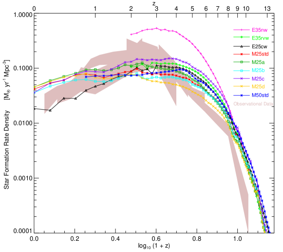
The global star formation rate density (SFRD) as a function of redshift is plotted in Fig. 1, with the nine runs labelled by the different colours and plotting symbols. The SFRD (in yr-1 Mpc-3) is computed by summing over all the SF occurring in each simulation box at a time, and dividing it by the time-step interval and the box volume. Observational data ranges are shown as the grey shaded region, taken mainly from Cucciati et al. (2012), and the compilations therein originally from Perez-Gonzalez et al. (2005), Schiminovich et al. (2005), Bouwens et al. (2009), Reddy & Steidel (2009), Rodighiero et al. (2010), van der Burg, Hildebrandt & Erben (2010), Bouwens et al. (2012).
SN feedback clearly has a significant impact on the SFRD; compared to E35nw, SF is reduced by a factor of several in the other runs at . The stronger kinetic feedback runs (M25b and M25d) quench SFR more than the others. In fact, case M25d produce the lowest SFRD from high- up to , but at run E25cw has the lowest SFRD. Among the feedback runs, M25c produces the highest SFRD; implying that a probability of kicking gas particles into wind yields the least efficient kinetic feedback.
The scatter in the SFRD values within the MUPPI runs are larger at , and reduces at due to overall gas depletion. The SFRD is higher in M50std than in M25std from high- up to , and becomes comparable later. This is because, despite having the same parameter values and resolution, runs M50std and M25std uses different cooling functions (§2.1).
At earlier cosmic epochs , the SFRD in the simulations is systematically higher, reaching times the observed values. Later at , most of the models overall lie within the ranges of SFRD produced by the different observations. However at , the MUPPI models produce a higher and the Effective model a lower SFRD than the observations. The low- discrepancy is because we do not have AGN feedback, which when present is expected to quench additional SF, bringing the MUPPI models closer to observations. Studying the shape evolution, most of the simulations reach a maximum SFRD in the form of a plateau between , and the SFRD decreases steeply at and gradually at . This is contrary to the peak of observed SFRD at .
We compare our results with two contemporary cosmological hydrodynamical simulations. At the SFRD in our simulations is higher than that obtained in (Vogelsberger et al., 2014), our SFRD exhibits a plateau maximum and not a well-defined peak at like them, and at also our SFRD is higher. Our results are more akin to that of some runs in (Schaye et al., 2010) which show a SFRD plateau between .
4.2 Single Galaxy
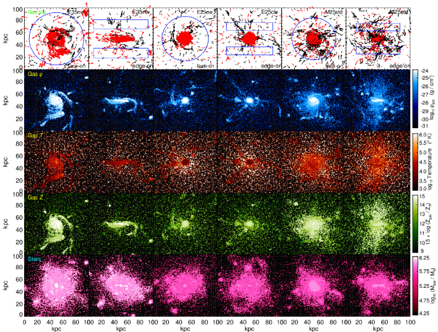
The gas distribution of a massive galaxy of total mass (left two columns) and (remaining columns) at is plotted in Fig. 2 for three runs. Each of the five rows shows a gas/star property, projected in the face-on (left) and edge-on (right) planes of a kpc volume. First row depicts the velocity vectors of gas particles, with the outgoing () particles denoted as red, and incoming () gas as black. Here the blue circle in the face-on panels and the double blue rectangles in the edge-on panels illustrate the projected bi-cylinder volume used to measure the outflow (§3.1) of each galaxy. Gas density is in the second row, temperature in the third, and total metallicity is plotted in the fourth row.
E35nw and M25std present the formation of a gas disk with extended spiral arms and tidal features. In the no-wind case E35nw, the gas disk is bigger in size, more massive, more metal enriched; and there is no prominent outflow. While in run E25cw the central gas distribution is spheroidal, and most of the outflowing gas lies inside kpc, because here the wind kick velocity km/s is too small to drive large-scale outflows. The Muppi run M25std produces a well-developed gas outflow propagating perpendicular to the galaxy disk, escaping to kpc from the galaxy center. Metals are more distributed in runs E25cw and M25std, since SN winds carry the metals out from the SF regions and enrich the CGM. The fourth row also shows that the M25std outflow (right two panels) is more metal enriched at kpc from the galaxy, than the E25cw case (middle two panels). Stellar mass in the bottom row reveals a central disk-like structure, surrounded by a larger stellar halo. The stellar disk is thinner in the no-wind case E35nw, than in the MUPPI run M25std.
4.3 Outflow Properties of Galaxies at
We measure the gas outflow properties of galaxies using the bi-cylinder technique described in §3.1, with a limiting velocity both fixed and scaled with , by analysing central galaxies having . The results of all the nine simulations at are presented in this section.
We study the trends of outflow and with basic galaxy properties: (i) halo mass, (ii) gas mass, (iii) stellar mass, (iv) SFR (sum of all the instantaneous star formation occurring in the gas belonging to a galaxy), (v) gas consumption timescale = gas mass / SFR, (vi) star formation timescale = stellar mass / SFR; attempting to find possible correlations. We find positive correlations of the outflow quantities with galaxy mass and SFR. However the correlation with galaxy SFR is the tightest, hence we present only these here.
4.3.1 Outflow Velocity
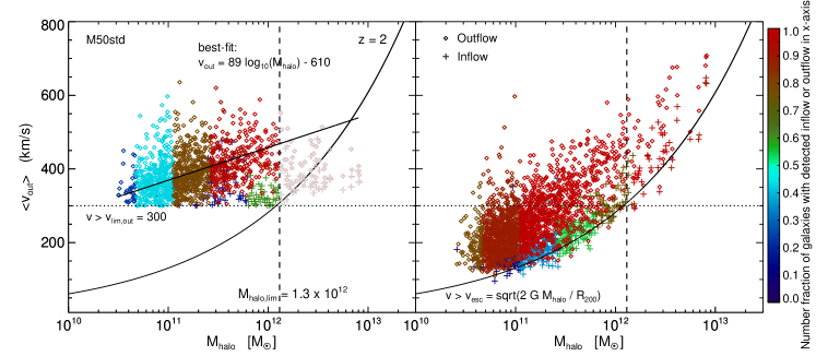
The velocity of outflow, , as a function of halo mass of galaxies in run M50std is plotted in Fig. 3, illustrating the two different methods of computing . Outflowing gas particles are selected when their -velocity component is above: (i) a constant limiting speed or km/s (Eq. 10) in the left panel, and (ii) the escape velocity or at the right, as described in §3.1. As a test we present the inflows: gas particles having velocities over the threshold and , as well in this figure. The flow direction is indicated by the plotting symbols: outflows as diamonds, and inflows as plus symbols. The plotting colour depicts the number fraction of galaxies where outflow or inflow is detected in bins of halo mass. The grey points in the left panel (includes both outflow and inflow) mark galaxies more massive than (vertical black dashed line). In the right panel the inflow velocities are spread very close to the curve, because inflows consist of thermal velocity and random motion of the gas, and by imposing a lower cutoff of we measure the motion occurring close to . Whereas most the outflow velocities are larger (by a few times) than at all halo masses; which demonstrates that we are measuring non-thermal gas outflow driven by stellar and SN feedback processes. The left panel, by selecting gas above a fixed cutoff of km/s, shows a positive correlation of the measured outflow velocity with halo mass.
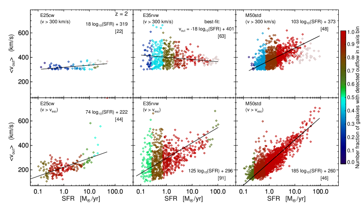
The outflow velocity as a function of SFR of galaxies is plotted in Fig. 4 for three runs, illustrating the two different methods of computing outflow in the two rows. The plotting colour depicts the number fraction of galaxies where outflow is detected in bins of SFR, as indicated by the colorbar on the right. The differences between the two rows is the largest for the Effective models E25cw and E35rvw (left two columns), because these runs have energy-driven wind where is not dependent on galaxy mass. E25cw has km/s, and using a fixed lower cutoff of km/s selects only a few gas particles in the lower-mass galaxies. For the MUPPI run M50std, the two distinct lower cutoffs make a small difference.
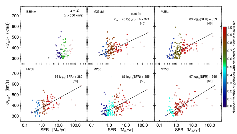
Fig. 5 presents the outflow velocity as a function of SFR of galaxies for the six remaining simulations, where outflow is measured by selecting gas above a fixed km/s. The grey points mark galaxies more massive than , where the outflows might not escape the halo potential.
We see that kinetic SN feedback is needed to generate an outflow in the lower-SFR (consequently less-massive) galaxies. Therefore the no-wind run E35nw shows outflowing gas only in some galaxies with SFR yr; this can be interpreted as the expected contamination from gravity-driven gas flows, and is roughly consistent with the statistics of inflows in the left panel of Fig. 3. In the other runs more than galaxies with SFR yr have outflows. The number fraction of galaxies where outflow is detected (indicated by the plotting colour) increases with galaxy SFR.
All the runs, except E25cw, present a large scatter. The Effective models produce, with low probability, an outflow velocity which shows no relation with SFR. Run E25cw has a constant km/s, since the input model is energy-driven wind with a fixed km/s. Run E35rvw has a large scatter with km/s. It uses a radially varying wind of velocity (Eq. 4) with the speed going up to km/s at kpc. This turns out to be a strong wind for the low-SFR galaxies, where km/s is reached.
The six MUPPI runs (five in Fig. 5 and one in Fig. 4) display a positive correlation of with galaxy SFR: rising from km/s at low-SFR to km/s at high-SFR. It is the most steep in the larger-box run M50std, which has the highest number of galaxies. The positive correlation has the largest scatter in M25c, the least efficient kinetic feedback case with a probability of kicking gas particles into wind.
4.3.2 Mass Outflow Rate

The mass outflow rate, from Eq. (11) in §3.1, as a function of SFR of galaxies, is plotted in Fig. 6 for three runs, illustrating the two different methods of computing outflow in the two rows. Gas particles are selected above: (i) a constant limiting speed km/s in the top row, and (ii) the escape velocity at the bottom. It is physically expected that gas moving faster than is able to escape the galaxy halo; therefore the bottom row gives a physically motivated estimate of the outflowing mass that can make its way out of the halo. The differences between the two rows is the largest for run E25cw in the left column; because it has energy-driven wind with km/s, and using a fixed lower cutoff of km/s selects only a few gas particles in the lower-mass galaxies. For the other two runs with strong kinetic feedback: E35rvw and M50std, the two distinct lower cutoffs make very small difference.
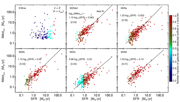
The mass outflow rate as a function of SFR of galaxies for the six remaining simulations is plotted in Fig. 7. The format is same as the bottom row of Fig. 6, where gas is selected above the escape velocity . The plotting colour depicts the number fraction of galaxies where outflow is detected in bins of galaxy SFR.
The no-wind run E35nw presents outflow in a few high-SFR galaxies only, and shows a scatter having no relation with the SFR. The two Effective models with kinetic SN feedback (Fig. 6) display a weak positive correlation of and galaxy SFR, having a value of slope , which is flatter than the MUPPI models. E25cw has a larger scatter than E35rvw.
4.3.3 Mass Escape at Virial versus Galaxy Radius
| Method | ||
|---|---|---|
| At using , in a cylinder | ||
| At using , in a sphere | ||
| At using , in a sphere |
We compare outflow measurements at using the cylinder and the sphere techniques, which reveal us their shapes. During propagation an outflow could be slowed down by hydrodynamical interactions with neighbouring gas. In order to estimate what mass fraction can escape the halo gravitational potential, we compare the rates by measuring outflow at the galaxy radius and that at the virial radius .
Here we present results of run M50std at by analysing central galaxies, among a total of galaxies with . Table 2 lists the number of outflows detected using different methods at two radii: in the first two rows, and in the third row. We find that the fraction of galaxies where outflow is detected at is using the cylinder method, and rises to using the sphere technique. We furthermore find that the outflow detection fraction decreases from at , to at . The reduction factor is small; among the outflows which escape the galaxy, can escape the halo as well.
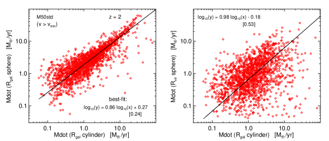
Fig. 8 presents the mass outflow rate in run M50std at measured by different techniques; left panel: at the galaxy radius in a sphere versus that at in a cylinder, and right: at the virial radius in a sphere versus that at in a cylinder. Outflows are measured by selecting gas particles above the escape velocity at the given radius. There is a substantial scatter in the right panel, with varying up to a few ’s at the same ; however a clear positive correlation is visible. The black line shows the result of an outlier-resistant two-variable linear regression. In the right panel, this gives the best-fit relation of the mass escape at the two radii: . From the left panel and the detection number ratio in the previous paragraph we conclude that, the shape of the outflow is bi-polar in galaxies.
4.3.4 Mass Loading Factor
We compute the outflow mass loading factor by taking the ratio of the mass outflow rate (measured at using the bi-cylinder method) with galaxy SFR,
| (13) |
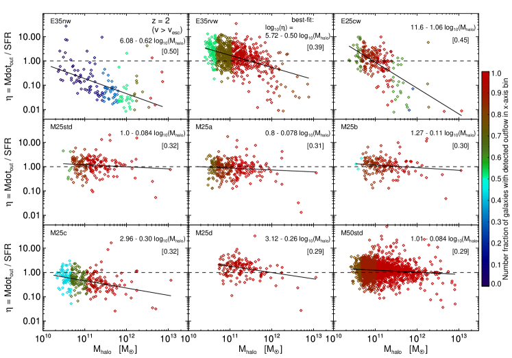
Fig. 9 presents as a function of halo mass of galaxies for all nine simulations, using a format same as Fig. 7. The outflowing gas is selected above the escape velocity . The plotting colour depicts the number fraction of galaxies where outflow is detected in bins of halo mass. All the runs exhibit a scatter, with varying up to factors of some-’s at the same halo mass.
The Effective model cases (E35nw, E25cw and E35rvw at higher masses) generate a negative correlation of with . This is because two runs have kinetic SN feedback in the energy-driven outflow formalism (§2.3), where the wind kick velocity is fixed over all galaxy masses. The result turns out to be a strong wind for the low-mass galaxies, where a large amount of gas is expelled compared to SF, reaching . On the other hand, it is a weak wind for the high-mass galaxies, where little gas is expelled and . At lower masses (), run E35rvw shows a constant scattered between versus .
All the six MUPPI runs display an almost constant value of over the full range of . The mass loading factors in most of the MUPPI galaxies lie between , with an average value of .
4.3.5 Implications and Comparison with Theoretical Estimates
We find that the MUPPI model is able to produce galactic outflows whose velocity and mass outflow rate correlates positively with global properties of the galaxy (halo mass, SFR). This is achieved with MUPPI using fully local properties of gas as input to the sub-resolution model. This trend, tracing some of the global properties of galaxy using local properties of gas, is found for the first time in cosmological simulations using sub-resolution models. We decipher that such trends arise from the details of the MUPPI sub-resolution model. Here star formation depends on local pressure through the molecular fraction of gas (Eq. 5 in Murante et al. 2010), and the gas pressure is expected to depend on halo mass. The star forming gas undergoes kinetic feedback and produces galactic outflows. Therefore consequently the outflow properties become dependent on halo mass and other global properties, through the local gas pressure.
On the other hand, the Effective model imparts a constant velocity to the gas, and a constant mass-loading , as input to the sub-resolution recipe. Consequently, the measured outflow speed is seen to be constant in the Effective model. However it produces a trend of decreasing (from a value of to ) with halo mass, and is only achieved for a narrow range of galaxy masses.
The results we obtain here by computing outflows in galaxies extracted from cosmological hydrodynamical simulations, can be compared to theoretical estimates of the MUPPI sub-resolution model. At variance with other kinetic wind recipes in the literature, in MUPPI neither the wind mass loading factor nor the wind velocity are given as input quantities. Nevertheless, typical values of these can be estimated using certain hypothesis about the average properties of the gas, as done by Murante et al. (2014) in their Section 3.3. With the default parameter choices, the theoretical estimates are (Eq. 8 and Eq. 9 in §2.4): , and the mass-weighted average wind velocity km/s. However the exact values depend on the local dynamical time, hence in turn on the local gas properties.
The Muppi runs M25std and M50std yield outflow mass loading factor between , with an average value of , close to . The outflow velocity shows a positive correlation with galaxy mass and SFR, rising from km/s to km/s. Hence the simulation agrees with the theoretical estimate in higher-mass galaxies, but at lower-masses the outflow speed is smaller than km/s.
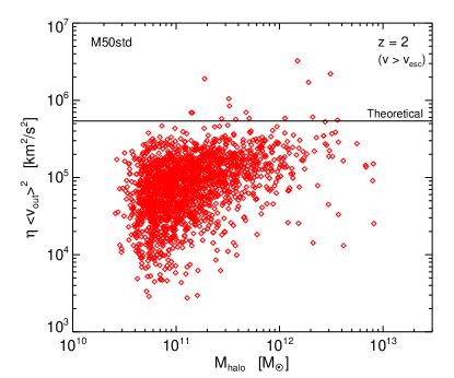
The product of mass loading factor and outflow velocity squared is predicted to be a constant in the MUPPI model (Murante et al., 2014): . This product for the simulated galaxies as a function of halo mass is plotted in Fig. 10 for run M50std. Here outflows are measured by selecting gas particles above the escape velocity . The horizontal black solid line marks the theoretical estimate km2/s2. The simulation results are lower than the theoretical prediction, especially in the less-massive galaxies. This is because the prediction assumes certain average properties of the gas. We in turn conclude that only a fraction rd of the deposited SN energy is used to drive an outflow; the rest being dispersed and radiated away through hydrodynamical interactions and by giving energy to slow particles.
4.4 Redshift Evolution of Outflows: from to
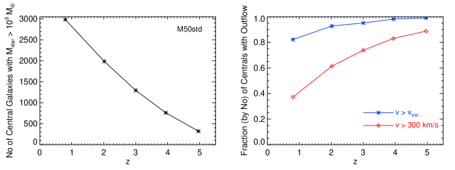
The outflow detection fraction of run M50std as a function of redshift is plotted in Fig. 11. Left panel shows the absolute number of central galaxies in simulation volume having a stellar mass . Right panel illustrates the number fraction of these centrals where outflow is detected (defined in Table 2), using the cylindrical volume methodology of §3.1. When outflow is measured by selecting gas above the escape velocity (, asterisks, blue curve), the outflow detection fractions are high at all epochs, reducing gradually from at , to at . When measured above a constant limiting speed ( km/s, diamonds, red curve), decreases from at , to at .
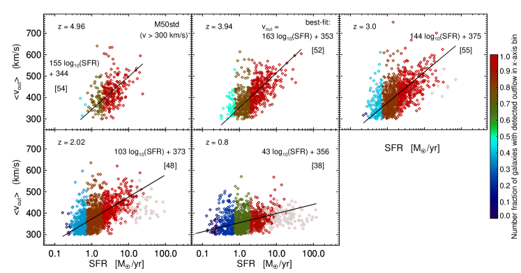
The redshift evolution of outflow velocity in simulation run M50std as a function of SFR of galaxies is plotted in Fig. 12. It shows the mass-weighted average, from Eq. (10) in §3.1. Each point is one galaxy, and the five panels show different redshifts. The remaining plotting format is the same as in Fig. 5. The correlation between and SFR is positive at all the explored epochs: steeper at earlier times, and becomes flatter at later epochs. The best-fit slope of (km/s) versus log10 (SFR/ yr are: at .
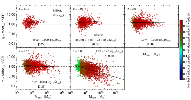
The redshift evolution of mass loading factor of galaxies in run M50std as a function of halo mass is plotted in Fig. 13. It shows from Eq. (13), as in Fig. 12, presenting the simulation at different epochs. In this figure the plotting colour depicts the number fraction of galaxies where outflow is detected in bins of halo mass. The value of exhibits a scatter at all the epochs, varying up to factors of at the same halo mass. Earlier on between , the galaxies have an almost constant value of over the full range of . The mass loading factors lie within , with an average value decreasing with the passage of time. At later epochs , displays a negative correlation with at the high-mass end.
The most important factor causing these redshift evolution of the outflow properties is the decrease of SFR at low- (§4.1). As seen in Fig. 1, the global SFRD in run M50std reaches a maximum between in the form of a plateau, with a steeper reduction of SFRD at earlier and later redshifts. This high SFR activity drives strong outflows in a greater fraction of galaxies, and causes the positive correlation of with SFR, as well as the constant- trend. Later at , SFR in galaxies reduce due to overall gas depletion, hence the driven outflows become weaker and rarer, and the outflow correlations are lost.
4.5 Comparison of Outflows with Observations and Other Models
Observational signatures of galactic outflows mostly comprise of single-galaxy detections. As a recent example at high redshift, Crighton et al. (2014) observed absorbing gas clumps in a galaxy CGM, produced by a wind with a mass outflow rate of yr. At low redshift, Cazzoli et al. (2014) detected kpc-scale neutral gas outflowing perpendicular to the disk of a galaxy, at a rate yr, with a global mass loading factor . Such values of mass outflow rate (a few to 10’s yr) and lie within our simulation result range (§4.3.2, §4.3.4).
Only over the last few years, observations of outflows in galaxy populations have been possible, and subsequent derivation of systematic trends. Grimes et al. (2009) detected starburst-driven galactic winds of temperature K in the absorption spectra of 16 local galaxies, and found that increases with both the SFR and the SFR per unit stellar mass. In a spectroscopic catalogue of 40 luminous starburst galaxies at , Banerji et al. (2011) inferred the presence of large-scale outflowing gas, with . Analysing the cool outflow around galaxies at , Bordoloi et al. (2013) found that (ranging between km/s) increases steadily with increasing SFR and stellar mass, and the wind is bipolar in geometry for disk galaxies. At low redshifts, Martin (2005) observed a positive correlation of outflow speed with galaxy mass in ultraluminous infrared galaxies at . Our simulations predict a positive correlation of with galaxy SFR and halo mass (§4.3.1), especially at (§4.4); hence consistent with all these observations.
Some galaxies in our simulations have a large km/s. This is in agreement with the high-velocity ( km/s) outflow observations by Karman et al. (2014) at in the UV spectra of massive galaxies. Our simulated trend that the outflow detection fraction decreases from to (§4.4), is consistent with that observed by Karman et al. (2014): the incidence of high- outflows () is much higher at massive galaxies than those at ; which is justified by the powerful SF and nuclear activity that most massive galaxies display at .
An earlier simulation work by Oppenheimer & Davé (2008) yielded galactic outflows with faster wind speeds at high- and slower winds at low-. This is in accord with our simulated redshift evolution of , which becomes weaker at (Fig. 12, §4.4). This trend, and the decrease of outflow detection fraction in our simulations from to later epochs, are in agreement with observations indicating that high- () galaxies almost ubiquitously reveal signatures of powerful winds (Veilleux, Cecil & Bland-Hawthorn, 2005), than those at lower-. We could not compare with the recent and simulations, because such outflow analysis has not been presented there. Our results are consistent with the recent work by Yabe et al. (2014), who employed a simple analytic model on an observational spectroscopic sample, and found that the gas outflow rate of star-forming galaxies decreases with decreasing redshift from to .
4.6 Radial Profiles of Gas Properties in Galaxies and their CGM at
The radial profiles of gas properties around galaxy centers at are presented in this section, considering all the galaxies (both centrals and satellites obtained by SubFind). Each property is shown as a function of galaxy radius, or distance from the location of subhalo potential minimum. All the non-wind gas particles lying inside a distance from the center are counted. The four panels denote total subhalo mass () ranges: (top-left) with number of subhalos in the different simulations within the range ; (top-right) having subhalos; (bottom-left) with subhalos; and (bottom-right) with subhalos.
All the subhalos within each mass range are stacked, and the plotted solid curves denote the median value in radial bins for each run. The shaded areas mark the region between th and th percentiles in runs E25cw (black curve) and M25std (red curve). It shows the typical scatter at a given radius, since galaxies do not have spherically-symmetric properties in general. The vertical dashed line is the virial radius for the following masses in the panels from top-left: , , , and , where the exact values are , and kpc respectively. The outer plotting radius is chosen to be twice the virial radius, or .
Wind particles, or gas particles which have recently received a velocity kick from kinetic SN feedback and are being decoupled from hydrodynamic interactions (§2.3, §2.4) are excluded while computing the profiles.
4.6.1 Density
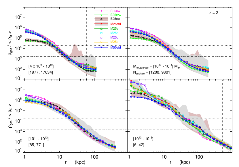
The gas overdensity (ratio of density to the mean baryon density) radial profiles are plotted in Fig. 14. Here the horizontal lines mark the SF threshold densities: cm-3 for the effective model (§2.3) as dotted, and cm-3 for the MUPPI model (§2.4) as dot-dashed. The gas denser than these thresholds in the respective models is forming stars. Within the approximate virial radius , all the gas density profiles can be roughly described by two power laws with a break at an intermediate radius of kpc, dependent on halo mass and wind model.
The inner parts kpc of the two lower subhalo mass ranges ( and , top two panels) present notable differences: E35rvw and E25cw runs produce a lower density, by times, than the others. The model input wind speed is independent of halo mass: constant km/s in E25cw, and that dependent on galactocentric radius, , in E35rvw. Such a velocity is high enough to eject the gas away from the halo potential in low-mass galaxies, making the inner density smaller in these two runs. The central gas is not able to escape in cases E35nw (no-wind) which has no kinetic SN feedback, and M25c which has less efficient feedback, therefore producing the highest gas density at galaxy cores than the other runs.
4.6.2 Temperature

The gas mass-weighted temperature radial profiles are presented in Fig. 15, in the same format as for density profiles. The average temperature has been used for those gas particles which are multiphase (star-forming). In all the effective model runs (E35nw, E35rvw, E25cw), the -profiles in the inner parts kpc of the galaxies follow the negative-sloped density-profiles (Fig. 14). This region contains dense gas forming stars at galaxy centers. The central gas undergoing SF has a warm to high temperature ( K) by construction, as a result of following the SF effective equation of state. The MUPPI model produces a colder ( K) galaxy core at kpc than the effective model.
There is a change in slope in the outer parts, at kpc in the top two panels, and at kpc in the bottom two panels; where the gas increases with radius, because of shock heating at galaxy outskirts. The -profiles in the two higher subhalo mass ranges ( and , bottom two panels) show a local peak at kpc, where the infalling gas collides with that in the halo and heats, to cool before reaching the center.
4.6.3 Metallicity
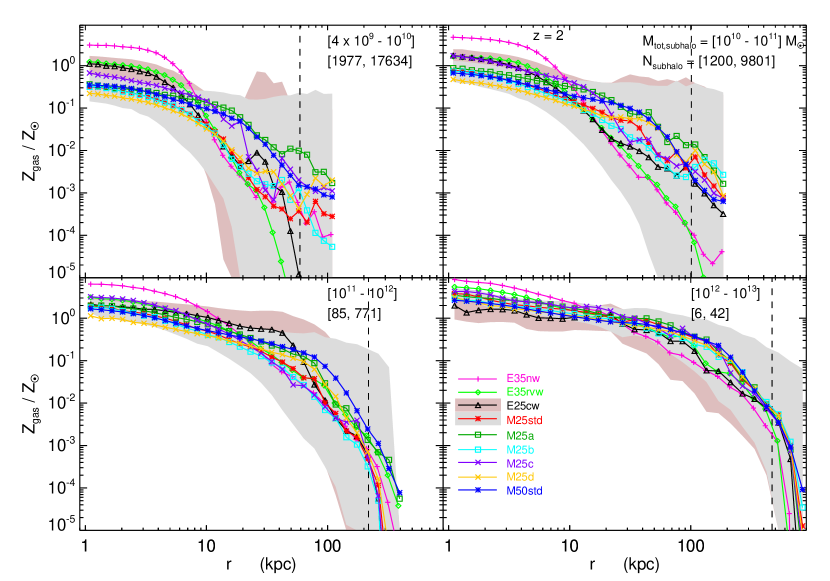
Radial profiles of gas total metallicity () are plotted in Fig. 16, showing the ratio of mass fraction of all metals in the gas to that of the Sun, . The solid curve medians and shaded area percentile values are computed considering all (both enriched and non-enriched) gas particles in radial bins. Some features of are similar to the gas density profiles (§4.6.1), because metals are produced during SF which occurs in dense regions. At all the profiles show decreasing going outward from center, with varying -dependent negative slopes.
All the MUPPI models produce relatively flatter metallicity profiles than the Effective models. Note that we do not use any metal loading factor in the sub-resolution recipe of any model. Gas particles carry away all of the metals they contain, and pollute the CGM. The no-wind run E35nw, which has no kinetic SN feedback, has the highest metallicity in the inner kpc. Wind feedback in the other runs suppresses central SF and transports some metal out, lowering the central . The trend reverses in the outer kpc: the kinetic feedback runs attain a higher than E35nw, because of accumulation of metal-enriched gas expelled by wind. The differences are most prominent in the lower subhalo mass ranges ( and , top two panels), and decreases at higher masses.
We infer that MUPPI distributes metals more adequately than the Effective models, which was already seen for a single galaxy in Fig. 2, fourth row.
4.6.4 Comparison of Radial Profiles with Other Works
Performing zoom-in simulations of Milky-Way-mass disc galaxy formation, Hummels et al. (2013) and Marinacci et al. (2014) computed the radial profiles of diffuse CGM gas properties. Our density profiles (§4.6.1, Fig. 14) and metallicity profiles (§4.6.3, Fig. 16) are qualitatively similar to these studies. Our density profiles are also consistent to a work by Pallottini, Gallerani & Ferrara (2014). Our -profiles (§4.6.2, bottom two panels of Fig. 15) present a local peak at kpc, which is at a larger- than the peak of Hummels et al. (2013). Our -profiles are qualitatively consistent with observations which show breaks (changes of slope) in the radial metallicity profiles, and/or rising metallicity gradients in the outer regions of galaxies (e.g., Scarano & Lepine, 2012).
5 Summary and Conclusion
We quantify the properties of galactic outflows and diffuse gas over by performing cosmological hydrodynamical simulations. We explore baryonic feedback models of star formation and SN feedback implemented within a modified version of the TreePM-SPH code GADGET-3. Our novel sub-resolution model MUPPI (Murante et al., 2010, 2014) incorporates SF in multiphase ISM, and a direct distribution of thermal and kinetic energy from SN to the neighbouring gas, using the free parameters of feedback energy efficiency fraction and a probability. For comparison with MUPPI, we adopt the Effective SF model (Springel & Hernquist, 2003) with variations of kinetic SN feedback, in the energy-driven formalism. Our simulations include additional sub-resolution physics: metal-dependent radiative cooling and heating in the presence of photoionizing background radiation; stellar evolution and chemical enrichment.
We compare a total of nine simulations in this paper, done using the concordance CDM model. We perform six new runs: five varying the SN feedback parameters of MUPPI, and one with the Effective model, of a Mpc comoving cosmological volume with DM and gas particles. An additional new MUPPI run is done of a larger Mpc box with particles, to increase the galaxy statistics. Two comparison simulations are taken from Barai et al. (2013): Effective SF model with no-wind and a radially varying wind case, which are Mpc boxes simulated with particles.
Identifying galaxies using the SubFind halo finder, we measure the gas outflow of each galaxy by tracking the high-speed gas particles belonging to it. Only the central galaxies having a stellar mass higher than are analysed. Our main findings are summarized below.
-
The star formation rate density shows that at the presence of kinetic SN feedback quenches SF more than any other feature of the SF model. The simulated SFRD has a plateau maximum between .
-
Kinetic SN feedback is able to drive gas and generate high-speed outflows in galaxies of all masses reached in our simulations, . It also creates inflows via deceleration and later fall back of gas between . Both the outflows and inflows are heated in massive galaxy halos. We find the following trends at :
-
When SN feedback is present, outflowing gas is detected in of the galaxies by number, depending on the model parameters and galaxy mass range. The number fraction of galaxies where outflow is detected increases with mass and SFR.
-
Some outflow characteristics (listed next) exhibit positive correlations with galaxy halo, gas and stellar masses, as well as with the SFR, which is the tightest. However most of the cases present a large scatter.
-
Measuring velocity of outflows by selecting gas above a fixed cutoff speed of km/s, the MUPPI model generates a positive correlation of with galaxy SFR, while the Effective model shows a constant with a large scatter.
-
Mass outflow rate is measured by selecting gas above the escape velocity. The MUPPI model presents a stronger and relatively tighter positive correlation of with galaxy SFR. The Effective model runs with kinetic SN feedback exhibit a weak positive correlation of with SFR, with a slope flatter than the Muppi models; E25cw has a larger scatter, and E35rvw a tighter correlation. The no-wind run E35nw displays a scatter of having no relation with the SFR.
-
The mass loading factor of the MUPPI outflows is constant with a scatter over all galaxy masses, , and an average . The Effective models generate a negative correlation of with . As an exception, run E35rvw presents a MUPPI-like trend at lower masses (): is constant between versus .
Hence the MUPPI model, using fully local properties of gas as input to the sub-resolution recipe, is able to produce galactic outflows whose velocity and mass outflow rate correlate with global properties of the galaxy (halo mass, SFR). This trend is found for the first time in cosmological simulations using sub-resolution models.
The Effective model results are caused by the input fixed wind kick velocity in the energy-driven formalism.
-
-
The shape of the outflows is inferred to be bi-polar in MUPPI galaxies. If outflowing gas can escape the galaxy radius, in cases it can escape the halo gravitational potential as well at the virial radius. The mass escape at the two radii are related as: .
-
The gas temperature radial profiles reveal that the MUPPI model produces a colder ( K) galaxy core at kpc than the Effective model.
-
The MUPPI model generates relatively flatter gas metallicity radial profiles than the Effective model.
-
-
The fraction of MUPPI galaxies exhibiting an outflow are high at all times between , when outflow is measured by selecting gas above the escape velocity. The outflow detection fraction decreases gradually at lower redshifts from at , to at .
The correlation between outflow velocity and SFR is positive at all the explored epochs: steeper at earlier times , and becomes flatter at later epochs. The mass loading factor is scattered within between , and the average decreases with the passage of time. Later at , displays a negative correlation with at the high-mass end. The reason is the high SFR at driving strong outflows in galaxies, while reduced SFR at later epochs quenches the outflow driving mechanism.
-
Our results are overall consistent with observations of galactic winds. Galaxy population observations indicate that increases with the SFR over , as we find in our simulations. Observations reveal that galaxies almost ubiquitously possess powerful winds, than those at lower-. This agrees with the decrease of outflow detection fraction in our simulations from to later epochs.
Our analysis demonstrates the ability of the MUPPI sub-resolution model to generate bi-polar outflows that present realistic properties. Additionally, we quantify the ability of both MUPPI and two variants of the standard energy-driven kinetic feedback model to produce significant outflows at of the virial radius and at the virial radius. Our study shows that, in the MUPPI model the fraction of energy really used to drive these outflows is only or less of that used by the code.
As future work we would like to extract more observable statistics from the simulations. In particular we want to explore IGM metal-enrichment, by computing the Lyman- flux and simulated quasar spectra, and compare them with observations of CGM and IGM at different impact parameters from galaxies. We also plan to peform better simulations in the future: run cosmological volumes with larger boxsize, and include AGN feedback in our models.
Acknowledgements
We are most grateful to Volker Springel for allowing us to use the GADGET-3 code. We thank Stefano Borgani, Gabriella De Lucia, David Goz, Michaela Hirschmann, Edoardo Tescari, and Luca Tornatore, for useful discussions. The simulations were partly carried out at the CASPUR computing center with CPU time assigned under two standard grants. Post-processing was done on the local machine lapoderosa, and we acknowledge partial support from “Consorzio per la Fisica - Trieste”. PB and MV acknowledge support from the ERC Starting Grant “cosmoIGM” and the INFN grant “INDARK”. GM and PM acknowledge support from the PRIN-INAF 2012 grant “The Universe in a Box: Multi-scale Simulations of Cosmic Structures”. PM acknowledges a FRA2012 grant from the University of Trieste.
References
- Aguirre et al. (2001) Aguirre, A., Hernquist, L., Schaye, J., Weinberg, D., H., Katz, N. & Gardner, J. 2001, ApJ, 560, 599
- Angles-Alcazar et al. (2014) Angles-Alcazar, D., Dave, R., Ozel, F. & Oppenheimer, B. D. 2014, ApJ, 782, 84
- Aracil et al. (2004) Aracil, B., Petitjean, P., Pichon, C. & Bergeron, J. 2004, A&A, 419, 811
- Arribas et al. (2014) Arribas, S., Colina, L., Bellocchi, E., Maiolino, R. & Villar-Martin, M. 2014, arXiv: 1404.1082
- Asplund, Grevesse & Sauval (2005) Asplund, M., Grevesse, N. & Sauval, A. J. 2005, in Barnes T. G., III, Bash F. N., eds, ASP Conf. Ser. Vol. 336, Cosmic Abundances as Records of Stellar Evolution and Nucleosynthesis. Astron. Soc. Pac., San Francisco, p. 25
- Banerji et al. (2011) Banerji, M., Chapman, S. C., Smail, I., Alaghband-Zadeh, S., Swinbank, A. M., Dunlop, J. S., Ivison, R. J. & Blain, A. W. 2011, MNRAS, 418, 1071
- Barai et al. (2013) Barai, P. et al. 2013, MNRAS, 430, 3213
- Baugh (2006) Baugh, C. M. 2006, Reports on Progress in Physics, 69, 3101
- Benson (2012) Benson, A. J. 2012, New Astronomy, 17, 175
- Bird et al. (2014) Bird, S., Vogelsberger, M., Haehnelt, M., Sijacki, D., Genel, S., Torrey, P., Springel, V. & Hernquist, L. 2014, arXiv: 1405.3994
- Bordoloi et al. (2013) Bordoloi, R. et al. 2014, ApJ, 794, 130
- Bouche et al. (2012) Bouche, N., Hohensee, W., Vargas, R., Kacprzak, G. G., Martin, C. L., Cooke, J. & Churchill, C. W. 2012, MNRAS, 426, 801
- Bouwens et al. (2009) Bouwens, R. J. et al. 2009, ApJ, 705, 936
- Bouwens et al. (2012) Bouwens, R. J. et al. 2012, ApJ, 754, 83
- Bradshaw et al. (2013) Bradshaw, E. J. et al. 2013, MNRAS, 433, 194
- Brook et al. (2005) Brook, C. B., Gibson, B. K., Martel, H. & Kawata, D. 2005, ApJ, 630, 298
- Brook et al. (2013) Brook, C. B., Stinson, G., Gibson, B. K., Shen, S., Maccio, A. V., Obreja, A., Wadsley, J. & Quinn, T. 2014, MNRAS, 443, 3809
- Burbidge, Burbidge & Rubin (1964) Burbidge, E. M., Burbidge, G. R. & Rubin, V. C. 1964, ApJ, 140, 942
- Burke (1968) Burke, J. A. 1968, MNRAS, 140, 241
- Cazzoli et al. (2014) Cazzoli, S., Arribas, S., Colina, L., Piqueras-Lopez, J., Bellocchi, E., Emonts, B. & Maiolino, R. 2014, arXiv: 1406.5154
- Cen & Ostriker (2000) Cen, R. & Ostriker, J. P. 2000, ApJ, 538, 83
- Chabrier (2003) Chabrier, G. 2003, PASP, 115, 763
- Chevalier & Clegg (1985) Chevalier, R. A. & Clegg, A. W. 1985, Nature, 317, 44
- Choi & Nagamine (2011) Choi, J.-H. & Nagamine, K. 2011, MNRAS, 410, 2579
- Crighton et al. (2014) Crighton, N. H. M., Hennawi, J. F., Simcoe, R. A., Cooksey, K. L., Murphy, M. T., Fumagalli, M., Prochaska, J. X. & Shanks, T. 2014, arXiv: 1406.4239
- Cucciati et al. (2012) Cucciati, O. et al. 2012, A&A, 539, A31
- Dalla Vecchia & Schaye (2008) Dalla Vecchia, C. & Schaye, J. 2008, MNRAS, 387, 1431
- Dalla Vecchia & Schaye (2012) Dalla Vecchia, C. & Schaye, J. 2012, MNRAS, 426, 140
- Dawson et al. (2002) Dawson, S., Spinrad, H., Stern, D., Dey, A., van Breugel, W., de Vries, W. & Reuland, M. 2002, ApJ, 570, 92
- Diamond-Stanic et al. (2012) Diamond-Stanic, A. M., Moustakas, J., Tremonti, C. A., Coil, A. L., Hickox, R. C., Robaina, A. R., Rudnick, G. H. & Sell, P. H. 2012, ApJ, 755, L26
- Dubois & Teyssier (2008) Dubois, Y. & Teyssier, R. 2008, A&A, 477, 79
- Fabbiano & Trinchieri (1984) Fabbiano, G. & Trinchieri, G. 1984, ApJ, 286, 491
- Fabjan et al. (2010) Fabjan, D., Borgani, S., Tornatore, L., Saro, A., Murante, G. & Dolag, K. 2010, MNRAS, 401, 1670
- Ferland et al. (1998) Ferland, G. J., Korista, K. T., Verner, D. A., Ferguson, J. W., Kingdon, J. B. & Verner, E. M. 1998, PASP, 110, 761
- Ford et al. (2013) Ford, A. B., Dave, R., Oppenheimer, B. D., Katz, N., Kollmeier, J. A., Thompson, R. & Weinberg, D. H. 2014, MNRAS, 444, 1260
- Fox et al. (2007) Fox, A. J., Ledoux, C., Petitjean, P. & Srianand, R. 2007, A&A, 473, 791
- Friedli & Benz (1995) Friedli, D. & Benz, W. 1995, A&A, 301, 649
- Frye, Broadhurst & Benitez (2002) Frye, B., Broadhurst, T. & Benitez, N. 2002, ApJ, 568, 558
- Gauthier & Chen (2012) Gauthier, J.-R. & Chen, H.-W. 2012, MNRAS, 424, 1952
- Goz et al. (2014) Goz, D., Monaco, P., Murante, G. & Curir, A. 2014, submitted to MNRAS
- Grimes et al. (2009) Grimes, J. P. et al. 2009, ApJS, 181, 272
- Haardt & Madau (2001) Haardt, F. & Madau, P. 2001, XXXVIth Rencontres de Moriond, XXIst Moriond Astrophysics Meeting, Editors D.M.Neumann & J.T.T.Van, 64
- Haas et al. (2013) Haas, M. R., Schaye, J., Booth, C. M., Dalla Vecchia, C., Springel, V., Theuns, T. & Wiersma, R. P. C. 2013, MNRAS, 435, 2931
- Heckman (2003) Heckman, T. M. 2003, Rev. Mex. Astron. Astrofis., 17, 47
- Hirschmann et al. (2013) Hirschmann, M. et al. 2013, MNRAS, 436, 2929
- Hummels et al. (2013) Hummels, C. B., Bryan, G. L., Smith, B. D. & Turk, M. J. 2013, MNRAS, 430, 1548
- Karman et al. (2014) Karman, W., Caputi, K. I., Trager, S. C., Almaini, O. & Cirasuolo, M. 2014, A&A, 565, A5
- Katz, Weinberg & Hernquist (1996) Katz, N., Weinberg, D. H. & Hernquist, L. 1996, ApJS, 105, 19
- Kawata (2001) Kawata, D. 2001, ApJ, 558, 598
- Kay, Thomas & Theuns (2003) Kay, S. T., Thomas, P. A. & Theuns, T. 2003, MNRAS, 343, 608
- Komatsu et al. (2011) Komatsu, E. et al. 2011, ApJS, 192, 18
- Kornei et al. (2012) Kornei, K. A., Shapley, A. E., Martin, C. L., Coil, A. L., Lotz, J. M., Schiminovich, D., Bundy, K. & Noeske, K. G. 2012, ApJ, 758, 135
- Kroupa, Tout & Gilmore (1993) Kroupa, P., Tout, C. A. & Gilmore, G. 1993, MNRAS, 262, 545
- Larson & Dinerstein (1975) Larson, R. B. & Dinerstein, H. L. 1975, PASP, 87, 911
- Lesgourgues et al. (2007) Lesgourgues, J., Viel, M., Haehnelt, M. G. & Massey, R. 2007, Journal of Cosmology and Astroparticle Physics, 11, 008
- Lewis et al. (2000) Lewis, A., Challinor, A. & Lasenby, A. 2000, ApJ, 538, 473
- Lundgren et al. (2012) Lundgren, B. F. et al. 2012, ApJ, 760, 49
- Marinacci et al. (2014) Marinacci, F., Pakmor, R., Springel, V. & Simpson, C. M. 2014, arXiv: 1403.4934
- Marri & White (2003) Marri, S. & White, S. D. M. 2003, MNRAS, 345, 561
- Martin (1999) Martin, C. L. 1999, ApJ, 513, 156
- Martin (2005) Martin, C. L. 2005, ApJ, 621, 227
- Mathews & Baker (1971) Mathews, W. G. & Baker, J. C. 1971, ApJ, 170, 241
- Monaco (2004) Monaco, P. 2004, MNRAS, 352, 181
- Monaco et al. (2012) Monaco, P., Murante, G., Borgani, S. & Dolag, K. 2012, MNRAS, 421, 2485
- Mori et al. (1997) Mori, M., Yoshii, Y., Tsujimoto, T. & Nomoto, K. 1997, ApJ, 478, L21
- Murante et al. (2010) Murante, G., Monaco, P., Giovalli, M., Borgani, S. & Diaferio, A. 2010, MNRAS, 405, 1491
- Murante et al. (2012) Murante, G., Calabrese, M., De Lucia, G., Monaco, P., Borgani, S. & Dolag, K. 2012, ApJ, 749, L34
- Murante et al. (2014) Murante, G., Monaco, P., Borgani, S., Tornatore, L., Dolag, K. & Goz, D. 2014, submitted to MNRAS
- Murray, Quataert & Thompson (2005) Murray, N., Quataert, E. & Thompson, T. A. 2005, ApJ, 618, 569
- Navarro & White (1993) Navarro, J. F. & White, S. D. M. 1993, MNRAS, 265, 271
- Newman et al. (2012) Newman, S. F. et al. 2012, ApJ, 752, 111
- Ohyama, Taniguchi & Terlevich (1997) Ohyama, Y., Taniguchi, Y. & Terlevich, R. 1997, ApJ, 480, L9
- Okamoto et al. (2005) Okamoto, T., Eke, V. R., Frenk, C. S. & Jenkins, A. 2005, MNRAS, 363, 1299
- Okamoto et al. (2010) Okamoto, T., Frenk, C. S., Jenkins, A. & Theuns, T. 2010, MNRAS, 406, 208
- Oppenheimer & Davé (2008) Oppenheimer, B. D. & Davé, R. 2008, MNRAS, 387, 577
- Oppenheimer et al. (2010) Oppenheimer, B. D., Davé, R., Keres, D., Fardal, M., Katz, N., Kollmeier, J. A. & Weinberg, D. H. 2010, MNRAS, 406, 2325
- Oppenheimer et al. (2012) Oppenheimer, B. D., Davé, R., Katz, N., Kollmeier, J. A., Weinberg, D. H., MNRAS, 2012, 420, 829
- Padovani & Matteucci (1993) Padovani, P. & Matteucci, F. 1993, ApJ, 416, 26
- Pallottini, Gallerani & Ferrara (2014) Pallottini, A., Gallerani, S. & Ferrara, A. 2014, accepted in MNRAS Letters, arXiv:1407.7854
- Perez-Gonzalez et al. (2005) Perez-Gonzalez, P. G. et al. 2005, ApJ, 630, 82
- Pettini et al. (2002) Pettini, M., Rix, S. A., Steidel, C. C., Adelberger, K. L., Hunt, M. P. & Shapley, A. E. 2002, ApJ, 569, 742
- Pinsonneault, Martel & Pieri (2010) Pinsonneault, S., Martel, H. & Pieri, M. M. 2010, ApJ, 725, 2087
- Piontek & Steinmetz (2011) Piontek, F. & Steinmetz, M. 2011, MNRAS, 410, 2625
- Puchwein & Springel (2012) Puchwein, E. & Springel, V. 2013, MNRAS, 428, 2966
- Rasera & Teyssier (2006) Rasera, Y. & Teyssier, R. 2006, A&A, 445, 1
- Reddy & Steidel (2009) Reddy, N. A. & Steidel, C. C. 2009, ApJ, 692, 778
- Rodighiero et al. (2010) Rodighiero, G. et al. 2010, A&A, 515, A8
- Rubin et al. (2010) Rubin, K. H. R., Weiner, B, J., Koo, D. C., Martin, C. L., Prochaska, J. X., Coil, A. L. & Newman, J. A. 2010, ApJ, 719, 1503
- Scannapieco et al. (2006) Scannapieco, C., Tissera, P. B., White, S. D. M. & Springel, V. 2006, MNRAS, 371, 1125
- Scannapieco et al. (2012) Scannapieco, C. et al. 2012, MNRAS, 423, 1726
- Scarano & Lepine (2012) Scarano, S. Jr. & Lepine, J. R. D. 2013, MNRAS, 428, 625
- Schaye et al. (2010) Schaye, J. et al. 2010, MNRAS, 402, 1536
- Schaye et al. (2014) Schaye, J. et al. 2014, submitted to MNRAS, arXiv:1407.7040
- Schiminovich et al. (2005) Schiminovich, D. et al. 2005, ApJ, 619, L47
- Sharma & Nath (2012) Sharma, M. & Nath, B. B. 2012, ApJ, 750, 55
- Shen et al. (2012) Shen, S., Madau, P., Aguirre, A., Guedes, J., Mayer, L. & Wadsley, J. 2012, ApJ, 760, 50
- Smith, Struck & Nowak (2005) Smith, B. J., Struck, C. & Nowak, M. A. 2005, AJ, 129, 1350
- Sommer-Larsen, Gotz & Portinari (2003) Sommer-Larsen, J., Gotz, M. & Portinari, L. 2003, ApJ, 596, 47
- Springel & Hernquist (2003) Springel, V. & Hernquist, L. 2003, MNRAS, 339, 289
- Springel (2005) Springel, V. 2005, MNRAS, 364, 1105
- Steidel et al. (2010) Steidel, C. C., Erb, D. K., Shapley, A. E., Pettini, M., Reddy, N., Bogosavljevic, M., Rudie, G. C. & Rakic, O. 2010, ApJ, 717, 289
- Steidel et al. (2011) Steidel, C. C., Bogosavljevic, M., Shapley, A. E., Kollmeier, J. A., Reddy, N. A., Erb, D. K. & Pettini, M. 2011, ApJ, 736, 160
- Stinson et al. (2006) Stinson, G., Seth, A., Katz, N., Wadsley, J., Governato, F. & Quinn, T. 2006, MNRAS, 373, 1074
- Stinson et al. (2007) Stinson, G. S., Dalcanton, J. J., Quinn, T., Kaufmann, T. & Wadsley, J. 2007, ApJ, 667, 170
- Sutherland & Dopita (1993) Sutherland, R. S. & Dopita, M. A. 1993, ApJS, 88, 253
- Tang et al. (2014) Tang, Y., Giavalisco, M., Guo, Y. & Kurk, J. 2014, accepted in ApJ, arXiv: 1407.0149
- Tescari et al. (2009) Tescari, E., Viel, M., Tornatore, L. & Borgani, S. 2009, MNRAS, 397, 411
- Tescari et al. (2011) Tescari, E., Viel, M., D’Odorico, V., Cristiani, S., Calura, F., Borgani, S. & Tornatore, L. 2011, MNRAS, 411, 826
- Tescari et al. (2014) Tescari, E., Katsianis, A., Wyithe, J. S. B., Dolag, K., Tornatore, L., Barai, P., Viel, M. & Borgani, S. 2014, MNRAS, 438, 3490
- Thacker & Couchman (2000) Thacker, R. J. & Couchman, H. M. P. 2000, ApJ, 545, 728
- Theuns et al. (2002) Theuns, T., Viel, M., Kay, S., Schaye, J., Carswell, R. F. & Tzanavaris, P. 2002, ApJ, 578, L5
- Thielemann et al. (2003) Thielemann, F.-K. et al. 2003, Nuclear Physics A, 718, 139
- Thompson et al. (2014) Thompson, T. A., Fabian, A. C., Quataert, E. & Murray, N. 2014, arXiv: 1406.5206
- Tornatore et al. (2004) Tornatore, L., Borgani, S., Matteucci, F., Recchi, S. & Tozzi, P. 2004, MNRAS, 349, L19
- Tornatore et al. (2007) Tornatore, L., Borgani, S., Dolag, K. & Matteucci, F. 2007, MNRAS, 382, 1050
- Vader (1986) Vader, J. P. 1986, ApJ, 305, 669
- van de Voort & Schaye (2012) van de Voort, F. & Schaye, J. 2012, MNRAS, 423, 2991
- van den Hoek & Groenewegen (1997) van den Hoek, L. B. & Groenewegen, M. A. T. 1997, A&AS, 123, 305
- van der Burg, Hildebrandt & Erben (2010) van der Burg, R. F. J., Hildebrandt, H. & Erben, T. 2010, A&A, 523, A74
- Vazza, Gheller & Bruggen (2014) Vazza, F., Gheller, C. & Bruggen, M. 2014, MNRAS, 439, 2662
- Veilleux, Cecil & Bland-Hawthorn (2005) Veilleux, S., Cecil, G. & Bland-Hawthorn, J. 2005, ARA&A, 43, 769
- Vikhlinin et al. (2009) Vikhlinin, A. et al. 2009, ApJ, 692, 1060
- Vogelsberger et al. (2014) Vogelsberger, M. et al. 2014, submitted to MNRAS, arXiv: 1405.2921
- von Glasow et al. (2013) von Glasow, W., Krause, M. G. H., Sommer-Larsen, J. & Burkert, A. 2013, MNRAS, 434, 1151
- Weil, Eke & Efstathiou (1998) Weil, M. L., Eke, V. R. & Efstathiou, G. 1998, MNRAS, 300, 773
- Weiner et al. (2009) Weiner, B. J. et al. 2009, ApJ, 692, 187
- Wiersma, Schaye & Smith (2009) Wiersma, R. P. C., Schaye, J. & Smith, B. D. 2009, MNRAS, 393, 99
- Wilman et al. (2005) Wilman, R. J., Gerssen, J., Bower, R. G., Morris, S. L., Bacon, R., de Zeeuw, P. T. & Davies, R. L. 2005, Nature, 436, 227
- Woosley & Weaver (1995) Woosley, S. E. & Weaver, T. A. 1995, ApJS, 101, 181
- Yabe et al. (2014) Yabe, K., Ohta, K., Akiyama, M., Iwamuro, F., Tamura, N., Yuma, S., Dalton, G. & Lewis, I. 2014, accepted in ApJ, arXiv: 1410.7147