Correlated starting points for the functional renormalization group

Abstract

We present a general frame to extend functional renormalization group (fRG) based computational schemes by using an exactly solvable interacting reference problem as starting point for the RG flow. The systematic expansion around this solution accounts for a non-perturbative inclusion of correlations. Introducing auxiliary fermionic fields by means of a Hubbard-Stratonovich transformation, we derive the flow equations for the auxiliary fields and determine the relation to the conventional weak-coupling truncation of the hierarchy of flow equations. As a specific example we consider the dynamical mean-field theory (DMFT) solution as reference system, and discuss the relation to the recently introduced DMF²RG and the dual-fermion formalism.

I Introduction

One of the main challenges in non-relativistic quantum many-body theory is the development of powerful tools for treating correlations between fermionic particles, not limited to specific parameter regimes. These would provide the keys for understanding and controlling many of the most exciting experiments currently performed in solid-state, nanoscopic- and cold-atoms physics. In fact, the state-of-the-art theoretical tools allow for an accurate treatment of quantum many-body correlations in specific cases, but their reliability is not guaranteed in general.

A very powerful method, among those currently available and widely used for performing model and realistic calculations of correlated fermions, is arguably the functional renormalization group (fRG) Salmhofer (1999); Berges et al. (2002); Kopietz et al. (2010); Metzner et al. (2012). The starting point of the fRG is an exact functional flow equation, which parametrizes the gradual evolution from an exactly solvable initial action ${\cal S}_{\rm ini}$ (typically of an uncorrelated problem) to the full final action ${\cal S}_{\rm fin}$ of the many-body problem of interest. Expanding the functional flow equation yields an exact infinite hierarchy of flow equations for the $n$-particle one-particle irreducible (1PI) vertex functions. However, for most calculations, the hierarchy of equations is truncated at the two-particle level. Because of this approximation, the validity of the conventional fRG is limited to the perturbative weak-coupling regime, except for situations in which phase space restrictions suppress higher order contributionsSalmhofer (1998); Salmhofer and Honerkamp (2001); Salmhofer (1999). For the same reason, the accuracy of the final results depends on the choice of the initial conditions.

In spite of the limitation to the weak-coupling regime, the fRG has led to powerful new approximation schemes: In fRG, infrared singularities can be dealt with much more efficiently than within the traditional resummations of perturbation theory, due to the built-in RG structure. Moreover, –differently from other perturbative approaches, such as RPA– fRG is ”channel-unbiased”: The fRG flow equations include the contributions of all scattering channels (e.g., spin, charge, particle-particle) and their reciprocal interplay.

The development of novel computation schemes for extending the advantages of an fRG-treatment to the strong-coupling regime, where e.g. Mott-Hubbard metal-insulator transitions can occur, represents a very challenging, but highly rewarding task. In fact, the potential of extending the fRG to the strong-coupling (SC) regime in order to overcome the main restriction of the conventional implementations has already motivated first pioneering studiesTaranto et al. (2014); Kinza et al. (2013); Kinza and Honerkamp (2013). The underlying idea is to access the SC regime by changing the initial conditions of the fRG flow: If these are extracted from the exact solution of a suitably chosen interacting reference problem, a significant part of the correlation effects are included non-perturbatively already from the very beginning, while the remaining ones will be generated, in all scattering channels, by the fRG flow. Formally, this corresponds to taking a SC ”reference” system ${\cal S}_{R}$ as an initial action ${\cal S}_{\rm ini}$, provided that it allows for a reliable (numerical or analytical) solution. In the case of the Anderson impurity model for example, the atomic-limit and extensions thereof have recently been used as a reference system to define a SC starting point for the fRG flowKinza et al. (2013); Kinza and Honerkamp (2013). For the Hubbard-model on the other hand, the effective AIM determined self-consistently by the dynamical mean-field theory (DMFT) was chosen to define the initial conditions of the fRG flowTaranto et al. (2014). This approach, coined DMF²RG, aims at a systematic and channel-unbiased inclusion of correlations,Taranto et al. (2014) beyond the purely local ones described, non-perturbatively, by the DMFT. We note that the idea of choosing a SC (or non-perturbative) reference system for the fRG flow has been recently introduced also in the context of spin-modelsRançon (2014); Reuther and Thomale (2014) or for systems of correlated bosonsRançon and Dupuis (2011a, b).

Irrespective of the performance in specific cases, all extensions of the conventional fRG face the challenge of proving the validity of the truncation procedures in the non-perturbative SC regime. This subject has never been explicitly addressed and calls for a systematic derivation.

The main goal of this paper is to define the properties of the fRG schemes with a non-perturbative starting point within a rigorous framework and a unified formalism. To this aim, we consider a general starting point for the perturbative expansion: performing a Hubbard-Stratonovich transformation for the fermionic degrees of freedom not associated to the chosen (SC) reference system, we derive an action in terms of the auxiliary Hubbard-Stratonovich fermionic fields (referred as ”dual” fermionsRubtsov et al. (2008); Brener et al. (2008); Hafermann et al. (2008); Rubtsov et al. (2009); Yang et al. (2011); Katanin (2013); Kirchner et al. (2013); Muñoz et al. (2013); Antipov et al. (2014) in the context of the diagrammatic extensionsHague et al. (2004); Toschi et al. (2007); Held et al. (2008); Rubtsov et al. (2008); Brener et al. (2008); Hafermann et al. (2008); Rubtsov et al. (2009); Valli et al. (2010); Yang et al. (2011); Katanin (2013); Kirchner et al. (2013); Muñoz et al. (2013); Rohringer et al. (2013); Antipov et al. (2014); Li (2014); Valli et al. (2014) of DMFT). The resulting equations are compared to those derived by directly working at the level of the physical fermions, and finally, the physical contents underlying the approximations made in the different schemes are critically analyzed.

The paper is organized as follows. In Sec. II we briefly review the general procedure for decoupling the fermionic degrees of freedom associated to a given reference system with the introduction of auxiliary fermions. The formulation in terms of auxiliary fields and its physical interpretation is presented in Sec. III. In Sec. VI we derive the flow equations in the auxiliary space and in Sec. V we discuss the relation to other methods. Finally, in Sec. VI, we summarize our results and draw conclusions.

II Interacting reference system

In the following, we present a general formalism that allows for an expansion around an interacting reference system. It was first introduced to set up an expansion of the $d$-dimensional Hubbard model around the atomic limit Pairault et al. (1998), and has recently been used in the dual-fermion (DF) formalism Rubtsov et al. (2008); Brener et al. (2008); Hafermann et al. (2008); Rubtsov et al. (2009); Yang et al. (2011); Katanin (2013); Kirchner et al. (2013); Muñoz et al. (2013); Antipov et al. (2014) to include non-local correlations beyond DMFT.

Let us start with a system of fermionic particles described by a general action of the form

$$\mathcal{S}(\bar{\varphi},\varphi) =-(\bar{\varphi},g^{-1}\varphi)+\mathcal{S}_{\rm{int}}(\bar{\varphi},\varphi).$$ (1)

Here we use the compact notation $(\bar{\varphi},\psi):=\sum_{\xi}\bar{\varphi}_{\xi}\psi_{\xi}$. $g$ denotes the non-interacting Green function, and $\mathcal{S}_{\rm{int}}$ contains quartic interaction terms in the Grassmann fields $\varphi_{\xi},\bar{\varphi}_{\xi}$. The multi-index $\xi=(\omega_{n},s)$ consists of a fermionic Matsubara frequency $\omega_{n}$ and a general quantum number $s$ including, e.g., momentum, spin and orbital index. We introduce an interacting reference system described by the action

$$\mathcal{S}_{R}(\bar{\varphi},\varphi) =-(\bar{\varphi},g^{-1}_{R}\varphi)+\mathcal{S}_{\rm{int}}(\bar{\varphi},\varphi)$$ (2)

written in terms of the same Grassmann fields as action (1). It differs from the latter only in the quadratic part $g^{-1}_{R}$, which is chosen such that the system is exactly solvable.

In order to expand the action

$$\mathcal{S}(\bar{\varphi},\varphi) =\mathcal{S}_{R}(\bar{\varphi},\varphi)-(\bar{\varphi},\Delta\varphi)$$ (3)

in the difference $\Delta=g^{-1}-g^{-1}_{R}$ of the quadratic parts, we cannot apply Wick’s theorem to the many-particle reference Green functions because the reference action $\mathcal{S}_{R}$ contains the quartic terms in the fields. Instead, we perform a fermionic Hubbard-Stratonovich transformation

$$(\bar{\varphi},nD^{-1}n\varphi)=\ln\int\frac{\mathcal{D}(\bar{\nu},\nu)}{\operatorname{det}D}e^{-(\bar{\nu},D\nu)+(\bar{\nu},n\varphi)+(\bar{\varphi},n\nu)},$$ (4)

introducing a set of auxiliary fermionic fields $\nu$, $\bar{\nu}$. We require that the matrices $n_{\xi,\xi^{\prime}}$ and $D_{\xi,\xi^{\prime}}$ fulfill the condition $nD^{-1}n=\Delta$, which implies freedom in the choice of $n$. At this point, we can perform the integration w.r.t. the physical fields $\varphi$, to yield an action

$$\mathcal{S}_{a}(\bar{\nu},\nu)=-(\bar{\nu},g^{-1}_{a}\nu)+\hat{\mathcal{V}}(\bar{\nu},\nu)$$ (5)

that depends on the auxiliary fields only (see Appendix B for more details), with an inverse Gaussian propagator

$$g^{-1}_{a}=-n\hskip 1.42271pt\left[G_{R}+\Delta^{-1}\right]\hskip 1.42271ptn$$ (6)

that contains correlation effects already through the one-particle Green function of the reference system $G_{R}$. The interaction of the auxiliary fields reads

$$\begin{split}\hat{\mathcal{V}}(\bar{\nu},\nu)=-\left[\ln\mathcal{G}^{R}(\bar{\eta},\eta)+(\bar{\eta},G_{R}\eta)\right]_{\begin{subarray}{c}\eta=n\nu\\ \bar{\eta}=n^{T}\bar{\nu}\end{subarray}}\end{split}$$ (7)

where $\mathcal{G}_{R}$ corresponds to the generating functional of the reference system Green functions

$$\mathcal{G}_{R}(\bar{\eta},\eta)=\frac{1}{Z_{R}}\int\mathcal{D}(\bar{\varphi},\varphi)e^{-[S_{R}(\bar{\varphi},\varphi)+(\bar{\eta},\varphi)+(\bar{\varphi},\eta)]}$$ (8)

with source fields $\eta$, $\bar{\eta}$. While the freedom in the choice of $n$ can be maintained in all following considerations, we focus on the conventional choiceRubtsov et al. (2008)

$$n=G_{R}^{-1}$$ (9)

for the sake of simplicity.

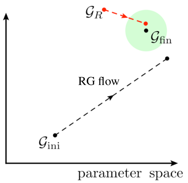
Figure 1: Schematic representation of the fRG flow in a general ”parameter space”. In conventional schemes the fRG flow starts from the generating functional of an uncorrelated problem $\mathcal{G}_{\mathrm{ini}}$. The approximations due to the truncation lead to deviations of the result at the end of the flow from the exact final generating functional $\mathcal{G}_{\mathrm{fin}}$. This truncation error can be reduced by using a correlated reference system (provided its generating functional $\mathcal{G}_{R}$ is exactly known) as a starting point for the flow.

Before providing more details about the treatment of the SC problem in auxiliary space, let us briefly sketch in Fig. 1 the idea motivating the formulation of an fRG flow from a SC starting point. In contrast to the case of the conventional fRG, the initial uncorrelated generating functional $\mathcal{G}_{\mathrm{ini}}$ is replaced by the one of the (solvable) interacting system, $\mathcal{G}_{R}$. A suitable choice reduces the effects of the truncation of the flow equations on the final result, which is therefore closer to the desired $\mathcal{G}_{\mathrm{fin}}$.

III The auxiliary problem

Now that we have reformulated our initial problem in terms of the auxiliary fields, we derive the expansion around the reference system solution. By definition the reference system solution is contained completely in the non-interacting theory ($\hat{\mathcal{V}}=0$) of the auxiliary fields, while any treatment of the auxiliary interaction introduces corrections that take into account the solution of the physical system. In the following, we discuss the physical interpretation of the propagator and of the interaction of the auxiliary fields, before introducing the relations between the physical quantities in auxiliary and physical space.

III.1 Gaussian propagator

The Gaussian propagator of the auxiliary fields (6) has interesting properties. We find that as $\Delta$ tends to zero, $g_{a}$ vanishes linearlyHafermann et al. (2009)

$$g_{a}\xrightarrow[\Delta\rightarrow 0]{}G_{R}\Delta G_{R}.$$ (10)

This means that any expansion in the interaction converges asymptotically, as higher order diagrams with $N$ internal lines will be suppressed as $\Delta^{N}$. For a physical intuition of the propagation described by $g_{a}$, we write

$$\begin{split}g_{a}&=\frac{1}{g^{-1}-\Sigma_{R}}-G_{R}.\end{split}$$ (11)

The first term can be interpreted as an approximation to the physical Green function (it actually brings the result of the 0th order expansion in $\hat{\mathcal{V}}$), from which we subtract the full reference propagator. In this sense, $g_{a}$ corresponds to the difference of the interacting propagators. Therefore it does not exhibit the typical $\sim 1/\omega$ behavior at large frequencies, but rather $\sim 1/\omega^{2}$.

III.2 Interaction

By integrating out the physical fields $\varphi$, the interaction of the auxiliary fields (7) is generated. It contains two- and multi-particle interactions that are given by the connected reference Green functions, where $G_{R}$ is amputated at each external leg. We can thus schematically write

$$\hat{\mathcal{V}}(\bar{\nu},\nu)= -\frac{1}{4}G^{(2),c}_{R}\left[\left(G_{R}^{-1}\bar{\nu}),\left(G_{R}^{-1}\bar{\nu}),(G_{R}^{-1}\nu\right),(G_{R}^{-1}\nu\right)\right]$$

$$-\frac{1}{9}G^{(3),c}_{R}\left[\left(G_{R}^{-1}\bar{\nu}),\left(G_{R}^{-1}\bar{\nu}),\left(G_{R}^{-1}\bar{\nu}),(G_{R}^{-1}\nu\right),(G_{R}^{-1}\nu\right),(G_{R}^{-1}\nu\right)\right]+...$$ (12)

where $G^{(m),c}_{R}$ ($m=2,\ldots,\infty$) denotes the connected $m$-particle reference Green function. In Eq. (12) we introduced the notation $V_{n}[a_{1},...,a_{n},a^{\prime}_{1},...,a^{\prime}_{n}]$ which is a shorthand for:

$$\begin{split}V_{n}[a_{1},...,a_{n},a^{\prime}_{1},...,a^{\prime}_{n}]_{\xi_{1},...,\xi_{n},\xi^{\prime}_{1},...,\xi^{\prime}_{n}}=(a_{1})_{\xi_{1},\psi_{1}}...\left(a_{n}\right)_{\xi_{n},\psi_{n}}V_{n}(\psi_{1},...,\psi_{n},\psi_{1}^{\prime},...,\psi_{n}^{\prime})\left(a^{\prime}_{1}\right)_{\psi_{1}^{\prime},\xi_{1}^{\prime}}...\left(a^{\prime}_{n}\right)_{\psi_{n}^{\prime},\xi_{n}^{\prime}},\end{split}$$ (13)

where we sum over repeated indices. $V_{n}$ represents a generic $n$-particle vertex function (e.g., connected Green’s function, 1PI vertex …) and $a_{i}$ is a two dimensional matrix in the multi index $\xi_{i}$.

Since the treatment of infinitely many multi-particle interactions poses an impossible task, approximations to the infinite series defining the interaction have to be devised. We drop the interaction terms beyond the quartic one and thus

$$\begin{split}\hat{\mathcal{V}}(\bar{\nu},\nu)\approx-\frac{1}{4}G^{(2),c}_{R}\left[\left(G_{R}^{-1}\bar{\nu}\right),\left(G_{R}^{-1}\bar{\nu}\right),\left(G_{R}^{-1}\nu\right),\left(G_{R}^{-1}\nu\right)\right]&=&-\frac{1}{4}\gamma_{2}^{R}[\bar{\nu},\bar{\nu},\nu,\nu],\end{split}$$ (14)

where $\gamma_{2}^{R}$ denotes the one-particle irreducible (1PI) two-particle vertex of the reference system. This represents an approximation based on the fundamental assumption that the effects of $(m\geq 3)$-particle scattering processes beyond the description of the reference system can be neglected. The impact this has on the resulting flow equations is discussed in Sec. IV. While previous worksPairault et al. (1998); Rubtsov et al. (2008); Brener et al. (2008); Hafermann et al. (2008); Rubtsov et al. (2009); Yang et al. (2011); Katanin (2013); Kirchner et al. (2013); Muñoz et al. (2013); Rohringer et al. (2013); Antipov et al. (2014) have treated the auxiliary interaction $\hat{\mathcal{V}}$ by means of perturbation theory or ladder approaches, we propose using the fRGMetzner et al. (2012) to perform a channel-unbiased resummation of diagrams to all orders in a scale-dependent fashion, thereby further improving on the physical results.

III.3 Relation to physical quantities

Once the solution in the auxiliary space is obtained, we need to translate Green- and vertex-functions from the auxiliary to the physical space. These relations can be formulated in a very general way by establishing the connection between the generating functionals. As shown in Appendix C, the generating functionals of the Green functions fulfill

$$\begin{split}\mathcal{G}(\bar{\eta},\eta)&=\mathcal{G}_{a}\left(G_{R}^{-T}\Delta^{-T}\bar{\eta},G_{R}^{-1}\Delta^{-1}\eta\right)\times e^{-(\bar{\eta},\Delta^{-1}\eta)},\end{split}$$ (15)

with $G_{R}^{-T}=\left(G_{R}^{-1}\right)^{\rm T}$. Further relations for the generating functional of the connected Green functions, or the effective interaction and the respective derivations are presented in Appendix C. By taking the derivative of Eq. (15) w.r.t. the source fields we find the relation between the physical and auxiliary Green functions

$$G=\Delta^{-1}+\Delta^{-1}G_{R}^{-1}G_{a}G_{R}^{-1}\Delta^{-1}.$$ (16)

Translated to the self energy, this relation reads

$$\Sigma=\Sigma_{R}+\frac{\Sigma_{a}}{\mathds{1}+G_{R}\Sigma_{a}},$$ (17)

where the fraction is to be understood as multiplication by the inverse from the right. The corresponding relation for the 1PI two-particle vertex reads (see Appendix C for further details)

$$\begin{split}\gamma_{2}=\gamma_{2,a}[\zeta,\zeta,\bar{\zeta},\bar{\zeta}],\end{split}$$ (18)

with $\zeta=\bar{G}^{-1}G_{R}$ and $\bar{\zeta}=G_{R}\bar{G}^{-1}$, where

$$\bar{G}=\left(g_{R}^{-1}-\Sigma\right)^{-1}.$$ (19)

In the following we refer to Eqs. (11), (17) and (18) and generalizations thereof for higher order vertices as the transformation to the auxiliary fields $\mathcal{T}$.

III.4 DMFT as reference system

To make the procedure described above more concrete, let us focus on the example of a reference system obtained by DMFT. This allows for a direct comparison with the DF approach and the recently introduced DMF²RG,Taranto et al. (2014) which is summarized in Sec. V.

DMFT can be considered the quantum extension of classical mean field theory Georges and Kotliar (1992); Georges et al. (1996) as it can be formally derived as the exact solution of a quantum lattice Hamiltonian in the limit of infinite spatial dimensions ($d\rightarrow\infty$) Metzner and Vollhardt (1989). In DMFT all non-local spatial correlations are averaged out, and one can reduce the study of a quantum lattice problem to a self consistently determined local impurity problem. For instance, one can consider the action of a one-band Hubbard model Hubbard (1963) given by

$$\mathcal{S}_{\rm lattice} =T\sum_{\omega_{n},\sigma}\int d{\mathbf{k}}\phantom{1}\bar{\varphi}_{\mathbf{k},\sigma}(\omega_{n})g^{-1}_{\mathbf{k}}(\omega_{n})\varphi_{\mathbf{k},\sigma}(\omega_{n})$$

$$\quad+U\sum_{i}\int d\tau\phantom{1}(n_{i,\uparrow}(\tau)-1/2)(n_{i,\downarrow}(\tau)-1/2),$$ (20)

with $T$ being the temperature, $g_{\mathbf{k}}^{-1}(\omega_{n})=(i\omega_{n}-\mu-\epsilon_{\mathbf{k}})$, $\epsilon_{\mathbf{k}}$ the energy dispersion of the lattice, $i$ the lattice site index, $U$ the Hubbard interaction and $n_{i,\sigma}(\tau)=\bar{\varphi}_{i,\sigma}(\tau)\varphi_{i,\sigma}(0)$. The on-site (local) properties of this action are studied in DMFT by singling out a lattice site and embedding it in an effective bath which accounts for the presence of all the other sites, i.e., an Anderson impurity model (AIM) in an effective bath. To guarantee that the AIM approximates the local physics of the lattice, the effective bath (or hybridization function) $\Gamma(\omega_{n})$ has to be computed self-consistently, and the resulting frequency dependence of the effective bath accounts for all purely local quantum correlations. The self-consistency condition that determines the effective bath and the propagator $g^{-1}_{\rm{imp}}(\omega_{n})=i\omega_{n}-\Gamma(\omega_{n})$ (often referred to as dynamical Weiss field in the DMFT literature) of the AIM reads:

$$G_{\rm{DMFT}}=\int d\mathbf{k}\hskip 2.84544pt\left(g_{\mathbf{k}}^{-1}-\Sigma_{\rm{DMFT}}\right)^{-1}=\left(g_{\rm{imp}}^{-1}-\Sigma_{\rm{DMFT}}\right)^{-1},$$ (21)

where $\Sigma_{\rm{DMFT}}$ is the self energy of the self-consistent impurity problem defined by $g_{\rm{imp}}$, and $G_{\rm{DMFT}}$ represents the DMFT approximation to the local interacting lattice Green’s function. The self-consistency equation (21) follows directly from the DMFT assumption of locality of the lattice self energy, which is clearly an approximation in finite-dimensional systems.

Since the AIM can be solved exactly, the action of a collection of disconnected self-consistent AIMs, one for each lattice site, is well suited as reference action to approximate the physical action (1)

$$\mathcal{S}_{R} =T\sum_{i,\omega_{n},\sigma}\bar{\varphi}_{i,\sigma}(\omega_{n})g^{-1}_{\rm{imp}}(\omega_{n})\varphi_{i,\sigma}(\omega_{n})$$

$$\quad+U\sum_{i}\int d\tau\phantom{1}(n_{i,\uparrow}(\tau)-1/2)(n_{i,\downarrow}(\tau)-1/2).$$ (22)

This way, the local physics of the system, computed at the DMFT level, is already included in the reference action. Note that assuming the action (22) as reference action is what is typically done in the DFRubtsov et al. (2008); Brener et al. (2008); Hafermann et al. (2008); Rubtsov et al. (2009); Yang et al. (2011); Katanin (2013); Kirchner et al. (2013); Muñoz et al. (2013); Antipov et al. (2014) approaches. In some cases, also the solution of a cellular DMFT Kotliar et al. (2001) or a Dynamical Cluster Approximation Hettler et al. (2000); Maier et al. (2005) calculation has been taken as a reference system Slezak et al. (2009); Yang et al. (2011). This way one is able to include non-perturbatively in the initial conditions also the short-range spatial correlations, providing a complementary multiscale Slezak et al. (2009) framework to treat correlations beyond DMFT over all length scales. Hence, the DF reference system is defined by the momentum-independent propagator $g_{\rm{imp}}$, while its interacting Green’s function is the local DMFT one

$$G_{R}^{-1}=g_{\rm{imp}}^{-1}-\Sigma_{\rm{DMFT}}.$$ (23)

Performing the Hubbard-Stratonovich transformation to introduce the auxiliary fermions relative to this reference system, one obtains for the non-interacting propagator

$$g_{a}=\frac{1}{i\omega_{n}-\epsilon_{\mathbf{k}}-\Sigma_{\rm{imp}}}-G_{R},$$ (24)

which explicitly depends on the momentum $\mathbf{k}$ through the lattice dispersion $\epsilon_{\mathbf{k}}$. The first term in Eq. (24) represents the DMFT approximation to the lattice Green’s function under the assumption of a local self energy. $g_{a}$ is also referred to as the purely non-local propagator, as the local impurity Green’s function is subtracted, and therefore it vanishes by summing over the momenta. As for the interaction between the auxiliary fields, this is, according to Eq. (14), given by the 1PI two-particle vertex of the AIMRubtsov et al. (2008). This input can be calculated Rohringer et al. (2012); Hafermann (2014) to high accuracy within the current numerical solvers for the AIM.

IV Flow equations

After having reformulated the initial problem by means of the auxiliary action (5) we now address the issue of solving this problem using the fRG. This procedure is sketched in the right-hand side of Fig. 2. Integrating the flow equations in auxiliary space (which are derived in the following) results in an approximated solution for the auxiliary problem that we can eventually translate back to acquire a physical solution. This scheme is then be compared to the one obtained by deriving fRG flow equations directly in the physical space.

Figure 2: Overview of the relation between the flow in physical and auxiliary space; $\mathcal{T}$ denotes the transformation to the auxiliary fields.

IV.1 General formulation

We recall that the first step to determine the fRG flow equationsMetzner et al. (2012) is to substitute the non-interacting propagator $g$ of the system in question by a scale-dependent $g^{\Lambda}$. This allows for the derivation of an exact functional flow equation that describes the gradual evolution of the effective action as the cutoff scale $\Lambda$ is changed. Expanding the flow equation in the 1PI vertex functions results in an infinite hierarchy of the form

$$\dot{\gamma}_{m}^{\Lambda}=f(\gamma_{1}^{\Lambda},\ldots,\gamma_{m}^{\Lambda},\gamma_{m+1}^{\Lambda}).$$ (25)

For practical implementations this hierarchy is typically truncated at the two-particle level by assuming that $\gamma_{3}^{\Lambda}\approx\gamma_{3}^{\Lambda_{\rm{ini}}}=0$, reducing the hierarchy to a set of coupled flow equations for the self energy and the 1PI two-particle vertex function

$$\dot{\Sigma}^{\Lambda} = -S^{\Lambda}\circ\gamma_{2}^{\Lambda}$$ (26)

$$\dot{\gamma}_{2}^{\Lambda} = \gamma_{2}^{\Lambda}\circ\left(S^{\Lambda}\circ G^{\Lambda}+G^{\Lambda}\circ S^{\Lambda}\right)\circ\gamma_{2}^{\Lambda}.$$ (27)

In Eqs. (26) and (27) the $\circ$ stands for summation over internal momenta and quantum numbers according to standard diagrammatic rules as shown explicitly in Appendix A, while

$$S^{\Lambda}=-G^{\Lambda}\left[\partial_{\Lambda}\left(g^{\Lambda}\right)^{-1}\right]G^{\Lambda}=\partial_{\Lambda}G^{\Lambda}|_{\Sigma^{\Lambda}\phantom{1}\mathrm{fix}}$$ (28)

denotes the single-scale propagator, with

$$G^{\Lambda}=\left[\left(g^{\Lambda}\right)^{-1}-\Sigma^{\Lambda}\right]^{-1}.$$ (29)

The scale dependence of $g^{\Lambda}$ has to be chosen such that, at the initial scale $\Lambda_{\rm{ini}}$, $\Sigma^{\Lambda_{\rm{ini}}}$ and $\gamma_{2}^{\Lambda_{\rm{ini}}}$ can be determined exactly, while the physical propagator $g$ is recovered at the final scale $\Lambda_{\rm{final}}$

$$g^{\Lambda_{\rm{final}}}=g.$$ (30)

In conventional fRG approaches the bare propagator vanishes at the beginning of flow. We introduce the notation

$$g^{\Lambda}=0\ldots g$$ (31)

to describe this scale-dependence. While this choice results in trivial initial conditions that can be read off from the microscopic model action directly, recent worksKinza and Honerkamp (2013); Kinza et al. (2013); Reuther and Thomale (2014); Taranto et al. (2014) introduced the idea of starting the fRG flow from a reference system solution by choosing

$$g^{\Lambda}=g_{R}\ldots g.$$ (32)

This approach corresponds to the left-hand side of Fig. 2.

IV.2 Flow in the auxiliary space

In contrast to the derivation in the previous subsection, we now consider the reformulated problem for the auxiliary fields, for which we set up an fRG flow in the conventional sense. For this, we introduce a scale dependent auxiliary field propagator $g_{a}^{\Lambda}=0\ldots g_{a}$. The resulting flow equations then read as Eqs. (26) and (27), where all physical objects have to be replaced by their auxiliary equivalents. Note that the relations (17) and (18) between the scale-dependent physical and auxiliary quantities remain valid. Even though the auxiliary self energy $\Sigma_{a}^{\Lambda}$ vanishes at the scale $\Lambda_{\rm{ini}}$, the initial conditions are in general highly nontrivial, since $\gamma_{2,a}^{\Lambda_{\rm{ini}}}=\gamma_{2}^{R}$.

As mentioned in Sec. III.2, we approximate the bare auxiliary interaction by its quartic term. This corresponds to neglecting the effect of multi-particle scattering processes when calculating corrections of the reference system solution towards the physical one. In the auxiliary fRG flow, this results in an initially vanishing scale-dependent three-particle vertex, $\gamma_{3,a}^{\Lambda_{\rm ini}}=\gamma^{R}_{3,c}=0$, which justifies our truncation of the auxiliary flow equation hierarchy. Note, however, that multi-particle scattering processes are of course included in the exact solution of our reference system, and thus in the initial conditions ($\gamma^{\Lambda_{\mathrm{ini}}}_{2,a}=\gamma^{R}_{2}$) of the flow. After solving these flow equations numerically, results have to be translated back, using the transformation $\mathcal{T}^{-1}$ as described in Sec. III.3.

This approach is similar in spirit to recent approachesKinza and Honerkamp (2013); Kinza et al. (2013); Reuther and Thomale (2014); Taranto et al. (2014) following Eq. (32), as depicted in the left-hand side of Fig. 2. In fact, any cutoff of the form (32) is translated to $g_{a}^{\Lambda}=0\ldots g_{a}$ in auxiliary space by means of (11). Without any approximations the two flow schemes yield identical results. The approximations due to the truncation the flow equation hierarchy however induce important differences, as illustrated in the following. We compare the two paths in Fig. 2 leading to a hierarchy of physical flow equations $\dot{\gamma}_{m}^{\Lambda}$. In particular, we will compare the equations for the one- and two-particle 1PI vertex functions as relevant to common truncation schemes. Assuming that the scale dependence $g_{a}^{\Lambda}$ translates into $g^{\Lambda}$ by (11), we determine the relation between the scale-dependent Green functions. Introducing the scale-dependence in Eq. (16) and solving for $G_{a}^{\Lambda}$ yields

$$G^{\Lambda}_{a}=\zeta^{\Lambda}\left(G^{\Lambda}-\bar{G}^{\Lambda}\right)\bar{\zeta}^{\Lambda},$$ (33)

where $\bar{G}$, defined by Eq. (19), acquires a scale dependence via $\Sigma^{\Lambda}$. For the single-scale propagator we use the definition $S_{a}^{\Lambda}=\partial_{\Lambda}G_{a}^{\Lambda}|_{\Sigma_{a}^{\Lambda}\phantom{1}\mathrm{fix}}$ to obtain

$$S_{a}^{\Lambda}=\zeta^{\Lambda}S^{\Lambda}\bar{\zeta}^{\Lambda}.$$ (34)

Considering that

$$\gamma_{2,a}^{\Lambda}=\gamma_{2}^{\Lambda}\left[\left(\zeta^{\Lambda}\right)^{-1},\left(\zeta^{\Lambda}\right)^{-1},\left(\bar{\zeta}^{\Lambda}\right)^{-1},\left(\bar{\zeta}^{\Lambda}\right)^{-1}\right],$$ (35)

we find that each diagram contributing to the auxiliary flow can be translated to its physical counterpart by making the substitutions

$$\begin{split}\gamma_{2,a}^{\Lambda}&\rightarrow\gamma_{2}^{\Lambda}\\ S^{\Lambda}_{a}&\rightarrow S^{\Lambda}\\ G^{\Lambda}_{a}&\rightarrow G^{\Lambda}-\bar{G}^{\Lambda}.\end{split}$$ (36)

To relate the flow equations for the self energy in the physical and auxiliary space we take the $\Lambda$-derivative of the scale-dependent Eq. (17)

$$\dot{\Sigma}^{\Lambda}=\zeta^{\Lambda}\dot{\Sigma}_{a}^{\Lambda}\bar{\zeta}^{\Lambda}.$$ (37)

Applying the translation rules above, the corresponding flow equation in physical space remains unchanged, and is thus given by Eq. (26). The flow equations for the two-particle vertex, instead, can be obtained by taking the $\Lambda$-derivative of Eq. (35). Besides the contribution arising by a direct translation of the diagrams in auxiliary space through Eq. (36), additional terms arise due to the derivative of the $\zeta^{\Lambda}$ factors attached at each leg

$$\dot{\gamma}_{2}^{\Lambda} =\dot{\gamma}_{2,a}^{\Lambda}\left[\zeta^{\Lambda},\zeta^{\Lambda},\bar{\zeta}^{\Lambda},\bar{\zeta}^{\Lambda}\right]-\gamma_{2,a}^{\Lambda}\left[\dot{\Sigma}^{\Lambda}G_{R},\zeta^{\Lambda},\bar{\zeta}^{\Lambda},\bar{\zeta}^{\Lambda}\right]$$

$$\quad-\gamma_{2,a}^{\Lambda}\left[\zeta^{\Lambda},\dot{\Sigma}^{\Lambda}G_{R},\bar{\zeta}^{\Lambda},\bar{\zeta}^{\Lambda}\right]-\gamma_{2,a}^{\Lambda}\left[\zeta^{\Lambda},\zeta^{\Lambda},G_{R}\dot{\Sigma}^{\Lambda},\bar{\zeta}^{\Lambda}\right]$$

$$\quad-\gamma_{2,a}^{\Lambda}\left[\zeta^{\Lambda},\zeta^{\Lambda},\bar{\zeta}^{\Lambda},G_{R}\dot{\Sigma}^{\Lambda}\right].$$ (38)

Finally, by truncating the auxiliary flow equation at the one-loop level, we get the following flow equations in physical space

$$\dot{\gamma}_{2}^{\Lambda} =\gamma_{2}^{\Lambda}\circ\left(S^{\Lambda}\circ G^{\Lambda}+G^{\Lambda}\circ S^{\Lambda}\right)\circ\gamma_{2}^{\Lambda}-\gamma_{2}^{\Lambda}\circ\left(S^{\Lambda}\circ\bar{G}^{\Lambda}+\bar{G}^{\Lambda}\circ S^{\Lambda}\right)\circ\gamma_{2}^{\Lambda}$$

$$\quad-\gamma_{2}^{\Lambda}\left[\dot{\Sigma}^{\Lambda}\bar{G}^{\Lambda},\mathds{1},\mathds{1},\mathds{1}\right]-\gamma_{2}^{\Lambda}\left[\mathds{1},\dot{\Sigma}^{\Lambda}\bar{G}^{\Lambda},\mathds{1},\mathds{1}\right]-\gamma_{2}^{\Lambda}\left[\mathds{1},\mathds{1},\bar{G}^{\Lambda}\dot{\Sigma}^{\Lambda},\mathds{1}\right]$$

$$\quad-\gamma_{2}^{\Lambda}\left[\mathds{1},\mathds{1},\mathds{1},\bar{G}^{\Lambda}\dot{\Sigma}^{\Lambda}\right],$$ (39)

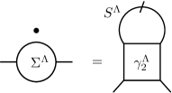
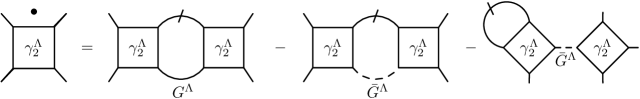
Figure 3: Diagrammatic representation of the physical flow equations for $\Sigma^{\Lambda}$ and $\gamma_{2}^{\Lambda}$ that correspond to solving the conventional flow equations for the auxiliary fields using the 2nd order truncation.

for a detailed derivation we refer to Appendix D. The corresponding diagrams are shown in Fig. 3. The first term of Eq. (39) is identical to the flow equation Eq. (27) for the two-particle vertex in physical space, while the other terms are not present in the conventional scheme. In particular, we note that the last four terms of Eq. (39) are reducible in $\bar{G}^{\Lambda}$. However, this ”reducibility” does not necessarily coincide with the reducibility in $G^{\Lambda}$ and could be attributed to the specific approximation performed here. This can also be understood by considering the relation between the physical and auxiliary scale-dependent three-particle vertices, depicted in Fig. 4. Assuming that the effect of $\gamma_{3,a}^{\Lambda}$ on the flow is negligible, we find that the effect of the physical 1PI three-particle vertex can be described by the effect of the rightmost term in Fig. 4. By connecting two of the six external (amputated) legs of this diagram with a single-scale propagator, one obtains the one-loop correction [second term in Eq. (39)] as well as the ”reducible” corrections [last four terms in Eq. (39)] to the conventional flow equation.

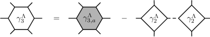
Figure 4: Relation between the physical and auxiliary scale-dependent three-particle vertex functions.

In particular, 1PI three-particle vertex corrections are included under the assumption that the auxiliary 1PI three-particle vertex vanishes. In conventional fRG, where it is assumed that both sides of the equation depicted diagrammatically in Fig. 4 do not contribute, three-particle vertex effects are fully neglected, unless they are explicitly accounted for, e.g., by two-loop diagramsKatanin (2004); Eberlein (2014). Let us note that a similar diagrammatic structure of the flow equations has been determined in a recent two-band fRG approachMaier and Honerkamp (2012), where a high-energy band was included perturbatively, resulting in an effective one-particle reducible three-particle interaction of the low-energy band. The corresponding contribution to the two-particle vertex flow was subsequently considered explicitly. We emphasize that in the present approach the one-particle ”reducible” (in the sense explained above) corrections to the physical self-energy inferred by (17) appear at the two-particle levelKatanin (2013) (as the last term in the flow equation for the vertex in Fig. 3). On the other hand, comparing the auxiliary flow equations to the ones obtained in the recently introduced 1PI approachRohringer et al. (2013), allows to attribute the one-particle ”irreducible” correction of the two-particle vertex to the the first two terms. Translated to the self-energy, for the Hubbard model with the DMFT as a starting point, these terms produce the analogue of the purely non-local contribution to the self-energy, which contains the Green function difference $G-\bar{G}$ in the diagrammatic series. In contrast, the contribution containing ”irreducible” diagrams with at least one internal $\bar{G}$-line of the 1PI approach is absent here, since the auxiliary three-particle vertex is neglected. For the half-filled $2d$ Hubbard model with the DMFT as a starting point, this approximation is justified at relatively strong coupling, where the respective contribution was found to be largely compensated by the contribution of the other channels Rohringer et al. (2013); Katanin (2009).

V Relations to other methods

The key idea presented in the previous sections is to approach the physical problem of treating strongly interacting fermions in a channel unbiased way in two essential steps: $i$) Setting up an expansion around a reference system solution by means of auxiliary fermions, and $ii$) solving the auxiliary problem by the fRG. Step $i$), first introduced in Ref. Pairault et al., 1998, is the basis of all the studies performed in the DF formalismRubtsov et al. (2008); Brener et al. (2008); Hafermann et al. (2008); Rubtsov et al. (2009); Yang et al. (2011); Katanin (2013); Kirchner et al. (2013); Muñoz et al. (2013); Antipov et al. (2014) as well as of the 1PI approachRohringer et al. (2013) and in the study of impurity systems within superperturbation theoryHafermann et al. (2009). An fRG flow from an interacting starting point, that is step $ii$), has been recently proposedKinza and Honerkamp (2013); Kinza et al. (2013); Rançon (2014); Reuther and Thomale (2014); Taranto et al. (2014).

To be more concrete, in the following, we concentrate on the cases where the DMFT solution is used as a reference system solution, which corresponds to the DF approaches regarding step $i$) and which has been also taken as direct input for the DMF²RG flow. This corresponds to take an action of the form of Eq. (22) as initial action and constructs the flow to the final action by interpolating the bare propagator from the AIM one, $g_{\rm imp}$, to the final (lattice) one, $g$. Differently to the auxiliary field method proposed here, however this is done directly in physical space. The important question to be addressed, then, is whether considering the flow in the auxiliary or in the physical space is more convenient. In DMF²RG, one is assuming that the effect of the DMFT three-particle 1PI vertex in correcting the self energy of the reference system is small compared to the effect of two-particle one. In the case of conventional fRG this can be justified, at least at weak coupling, by a power counting argumentSalmhofer and Honerkamp (2001) showing that the leading order contribution to the three-particle vertex is one order higher in the interaction compared to the leading one in the two-particle vertex. At intermediate-to-strong coupling, however, this argument does not apply anymore. Hence, in DMF²RG one should rely on the fact that the main contribution of the higher order vertex functions to the truncated fRG flow is already included in the initial condition as sketched in Fig. 1. Obviously, there is no guarantee that the effect of the three-particle 1PI vertex can be neglected in general. The difference with the approach discussed here in terms of the auxiliary fields is the following: In the present approach, the auxiliary three-particle vertex is neglected as discussed in Sec. IV (see schematic representation in Fig. 5). At the initial scale this corresponds to neglecting the connected reference three-particle vertex instead of the corresponding 1PI one.

Physical flow	Auxiliary flow
$g^{\Lambda}=g_{R}\ldots g$	$g^{\Lambda}_{a}=0\ldots g_{a}$
Effects of 1PI three-particle	Mimic 1PI three-particle
vertex fully neglected	vertex by means of

Figure 5: Effects of the truncation in the physical and auxiliary flow.

From the discussion above, it is clear that the crucial question is whether the physical 1PI three-particle vertex or the auxiliary one has a stronger effect on the corresponding flow. This certainly strongly depends on the problem under consideration and requires further focused investigations. Away from weak coupling this question is all but trivial, apart for some special cases, e.g., the Falicov-Kimball modelAntipov et al. (2014). Hitherto, due to its intrinsic numerical complexity, barely any knowledge about the three-particle quantities is available in the literatureHafermann (2010). A noticeable exception is the case of the Falicov-Kimball model, where it has been shown that the local auxiliary three-particle vertex $\gamma_{3,a}$ exactly vanishes in the particle-hole symmetric case. Here, however, perturbation theory considerations and the application of the Fury theorem Mandl and Shaw (2010) would suggest a simultaneous vanishing of the 1PI three-particle vertex for the physical fields. These results, however, cannot be directly extended to the Hubbard model. Therefore one has to critically analyze the results obtained with each approach and for each specific case. In order to compare with DF calculations, one can directly analyze the diagrammatic contributions in auxiliary space where the DF approachRubtsov et al. (2008); Brener et al. (2008); Hafermann et al. (2008); Rubtsov et al. (2009); Yang et al. (2011); Katanin (2013); Kirchner et al. (2013); Muñoz et al. (2013); Antipov et al. (2014) usually exploits perturbation theory or ladder resummations, as additional approximations. While one can not expect to capture diverging fluctuations by means of simple perturbation theory, ladder approaches are per definition biased towards a selected channel. On the other hand, by treating the auxiliary problem by means of the fRG one is able to treat competing scattering channels in an unbiased way. In particular, our approach allows for an improved computation of the solution of the auxiliary problem, including, although approximately, the parquet-approximation diagrams. Let us note that, differently from other non-perturbative schemesToschi et al. (2007); Held et al. (2008); Slezak et al. (2009); Valli et al. (2010, 2014), the calculations are based on the 1PI two-particle vertex, and do not require the two-particle irreducible (2PI) vertex at any point of the algorithm. This way one can circumvent the technical problems arising from the recently shown Yang et al. (2011); Schäfer et al. (2013); Janiš and Pokorný (2014) divergencies of the 2PI vertex at low frequencies, which are not associated with any thermodynamic transition.

VI Conclusion

We have demonstrated how the theory of an fRG-based expansion around a SC reference system can be rigorously formulated in the general framework of auxiliary fermionic variables. In particular, we have derived the explicit expressions for the fRG flow equations starting from a generic (exactly solvable) SC reference problem in the auxiliary fermionic fields and the corresponding transformation relations to calculate the physical quantities of the final solution. These derivations allow to clarify the relation to the fRG flow equations formulated directly for the physical fermionic fields, including the first pioneering ones reported in the recent literatureTaranto et al. (2014); Kinza et al. (2013); Rançon and Dupuis (2011a); Rançon (2014); Reuther and Thomale (2014). Furthermore, we could also elucidate the implications of the approximations introduced by truncating the hierarchy of the flow equations in the different schemes, see Fig. 5 for a summary. This represents indeed a pivotal aspect for all strong-coupling fRG algorithms, since the conventional arguments justifying the truncation does not hold any longer beyond the weak-coupling regime. Hence, a precise definition of the diagrammatic content associated to the truncation of a strong-coupling fRG flow is essential for adapting the novel algorithms to the non-perturbative physics of interest. The reported analytic and diagrammatic results, together with the physical insights which can be captured within the different formulations of the fRG with non-perturbative starting points, will provide an important reference for any future method development in this promising direction.

Appendix

VI.1 Notation details

Here we present explicitly Eq. (26) and Eq. (27), shown in compact notation in the main text. The flow equation for the self energy reads

$$\dot{\Sigma}(\xi_{1};\xi^{\prime}_{1})=-\frac{1}{\beta}\sum_{\omega_{2}}\sum_{s^{\prime}_{2},s_{2}}S^{\Lambda}_{s^{\prime}_{2};s_{2}}(\omega_{2})\gamma_{2}^{\Lambda}(\xi_{1},\xi_{2};\xi^{\prime}_{1},\xi^{\prime}_{2}).$$ (40)

We use the convention that for an $m$-particle quantity the first $m$ arguments refer to the outgoing lines, and the last $m$ to the incoming lines. The loop-variables are $\xi_{2}=(\omega_{2},s_{2})$ and $\xi^{\prime}_{2}(\omega^{\prime}_{2},s^{\prime}_{2})$. It is implicitly assumed that the energy is conserved ($\omega_{2}=\omega^{\prime}_{2}$), while the multi-index $s_{2}$ consists of a set of continuous and discrete quantum numbers. Therefore the summations $\sum_{s_{2},s^{\prime}_{2}}$ have to be understood as integrations or summations respectively. For example, in the case where only spin and momentum are considered for a translationally invariant system ($\mathbf{k}_{2}=\mathbf{k}^{\prime}_{2}$), Eq. (40) reads

$$\dot{\Sigma}(\xi_{1};\xi^{\prime}_{1})=-\frac{1}{\beta}\sum_{\omega_{2}}\sum_{\sigma_{2},\sigma^{\prime}_{2}}\int d\mathbf{k}\phantom{1}S^{\Lambda}_{\mathbf{k}^{\prime}_{2}\sigma^{\prime}_{2},\mathbf{k}_{2}\sigma_{2}}(\omega_{2})\gamma_{2}^{\Lambda}(\omega_{1}\mathbf{k}_{1}\sigma_{1},\omega_{2}\mathbf{k}_{2}\sigma_{2};\omega^{\prime}_{1}\mathbf{k}^{\prime}_{1}\sigma^{\prime}_{1},\omega^{\prime}_{2}\mathbf{k}^{\prime}_{2}\sigma^{\prime}_{2}).$$ (41)

For the 1PI two-particle vertex the flow equation is usually subdivided in three channels (particle-particle, particle-hole direct and particle-hole crossed) corresponding to the diagrammatic contributions

$$\dot{\gamma}_{2}^{\Lambda}(\xi_{1},\xi_{2};\xi^{\prime}_{1},\xi^{\prime}_{2})=\mathcal{C}_{pp}(\xi_{1},\xi_{2};\xi^{\prime}_{1},\xi^{\prime}_{2})+\mathcal{C}_{pp-d}(\xi_{1},\xi_{2};\xi^{\prime}_{1},\xi^{\prime}_{2})+\mathcal{C}_{ph-c}(\xi_{1},\xi_{2};\xi^{\prime}_{1},\xi^{\prime}_{2}),$$ (42)

with

$$\mathcal{C}_{pp}(\xi_{1},\xi_{2};\xi^{\prime}_{1},\xi^{\prime}_{2}) = \frac{1}{\beta}\sum_{\omega_{3}}\sum_{s_{3},s^{\prime}_{3},s_{4},s^{\prime}_{4}}\Big{[}S^{\Lambda}_{s^{\prime}_{3}s_{3}}(\omega_{3})G^{\Lambda}_{s^{\prime}_{4},s_{4}}(\omega_{1}+\omega_{2}-\omega_{3})+$$ (43)

$$G^{\Lambda}_{s^{\prime}_{3}s_{3}}(\omega_{3})S_{s^{\prime}_{4},s_{4}}^{\Lambda}(\omega_{1}+\omega_{2}-\omega_{3})\Big{]}\gamma_{2}^{\Lambda}(\xi_{1},\xi_{2};\xi^{\prime}_{3},\xi^{\prime}_{4})\gamma_{2}^{\Lambda}(\xi_{3},\xi_{4};\xi_{1}^{\prime},\xi_{2}^{\prime}),$$

$$\mathcal{C}_{ph-d}(\xi_{1},\xi_{2};\xi^{\prime}_{1},\xi^{\prime}_{2}) = -\frac{1}{\beta}\sum_{\omega_{3}}\sum_{s_{3},s_{3}^{\prime},s_{4},s_{4}^{\prime}}\Big{[}S^{\Lambda}_{s^{\prime}_{3}s_{3}}(\omega_{3})G_{s^{\prime}_{4},s_{4}}^{\Lambda}(\omega_{1}-\omega^{\prime}_{1}+\omega_{3})+$$ (44)

$$G^{\Lambda}_{s^{\prime}_{3}s_{3}}(\omega_{3})S_{s^{\prime}_{4},s_{4}}^{\Lambda}(\omega_{1}-\omega^{\prime}_{1}+\omega_{3})\Big{]}\gamma_{2}^{\Lambda}(\xi_{1},\xi_{3};\xi^{\prime}_{1},\xi^{\prime}_{4})\gamma_{2}^{\Lambda}(\xi_{4},\xi_{2};\xi^{\prime}_{3},\xi^{\prime}_{2}),$$

$$\mathcal{C}_{ph-c}(\xi_{1},\xi_{2};\xi^{\prime}_{1},\xi^{\prime}_{2}) = \frac{1}{\beta}\sum_{\omega_{3}}\sum_{s_{3},s_{3}^{\prime},s_{4},s_{4}^{\prime}}\Big{[}S^{\Lambda}_{s^{\prime}_{3}s_{3}}(\omega_{3})G_{s^{\prime}_{4},s_{4}}^{\Lambda}(\omega_{1}-\omega^{\prime}_{2}+\omega_{3})+$$ (45)

$$G^{\Lambda}_{s^{\prime}_{3}s_{3}}(\omega_{3})S_{s^{\prime}_{4},s_{4}}^{\Lambda}(\omega_{1}-\omega^{\prime}_{2}+\omega_{3})\Big{]}\gamma_{2}^{\Lambda}(\xi_{1},\xi_{3};\xi^{\prime}_{2},\xi^{\prime}_{4})\gamma_{2}^{\Lambda}(\xi_{2},\xi_{4};\xi^{\prime}_{1},\xi^{\prime}_{3}).$$

VI.2 Auxiliary fields

Performing the Hubbard-Stratonovich transformation (4) yields an action

$$\mathcal{S}(\bar{\varphi},\varphi,\bar{\nu},\nu)= \mathcal{S}_{R}(\bar{\varphi},\varphi)+\mathcal{S}_{\varphi}(\bar{\varphi},\varphi,\bar{\nu},\nu)+(\bar{\nu},n\Delta^{-1}n\nu),$$ (46)

with $\mathcal{S}_{\varphi}(\bar{\varphi},\varphi,\bar{\nu},\nu)=(\bar{\nu},n\varphi)+(\bar{\varphi},n\nu)$. We determine the interaction $\hat{\mathcal{V}}$ of the auxiliary $\nu$-fermions by integrating out the $\varphi$-fields and obtain

$$\int\mathcal{D}(\bar{\varphi},\varphi)e^{-\mathcal{S}_{R}(\bar{\varphi},\varphi)-\mathcal{S}_{\rm{\varphi}}(\bar{\varphi},\varphi,\bar{\nu},\nu)}=Z_{R}~{}e^{\,(\bar{\nu},\tilde{Q}\nu)-\hat{\mathcal{V}}(\bar{\nu},\nu)}.$$ (47)

This relation defines $\hat{\mathcal{V}}$ and $\tilde{Q}$, where $\tilde{Q}$ is to be chosen such that $\hat{\mathcal{V}}$ does not contain any quadratic part in the auxiliary fermions. Note that the l.h.s. is closely related to the generating functional of the reference Green functions

$$\int\mathcal{D}(\bar{\varphi},\varphi)e^{-\mathcal{S}_{R}(\bar{\varphi},\varphi)-\mathcal{S}_{\rm{\varphi}}(\bar{\varphi},\varphi,\bar{\nu},\nu)}=\left.Z_{R}\hskip 4.26773pt\mathcal{G}^{R}(\bar{\eta},\eta)\right|_{\eta=n\nu,\bar{\eta}=n^{T}\bar{\nu}}.$$ (48)

Inserting in Eq. (47) and solving for $\hat{\mathcal{V}}$ we obtain

$$\begin{split}\hat{\mathcal{V}}(\bar{\nu},\nu)=-\left[\ln\mathcal{G}^{R}(\bar{\eta},\eta)-(\bar{\eta},n^{-1}\tilde{Q}n^{-1}\eta)\right]_{\eta=n\nu,\bar{\eta}=n^{T}\bar{\nu}}=-\left[-(\bar{\eta},G_{R}\eta)+\mathcal{O}(\bar{\eta}^{2}\eta^{2})-(\bar{\eta},n^{-1}\tilde{Q}n^{-1}\eta)\right]_{\eta=n\nu,\bar{\eta}=n^{T}\bar{\nu}}.\end{split}$$ (49)

For the quadratic part of $\hat{\mathcal{V}}$ to vanish we have to choose $n^{-1}\tilde{Q}n^{-1}=-G_{R}$ and hence $\tilde{Q}=-nG_{R}n$. Thus

$$\begin{split}\hat{\mathcal{V}}(\bar{\nu},\nu)=-\left[\ln\mathcal{G}^{R}(\bar{\eta},\eta)+(\bar{\eta},G_{R}\eta)\right]_{\eta=n\nu,\bar{\eta}=n^{T}\bar{\nu}},\end{split}$$ (50)

in accordance with Eq. (7). This functional generates two-particle and multi-particle connected Green functions, where $n$ is appended at the outer legs. The free propagation of the auxiliary fields is then described by

$$Q_{a}=\tilde{Q}-n\Delta^{-1}n=-n\left[G_{R}+\Delta^{-1}\right]n$$ (51)

as shown in Eq. (6) for $Q_{a}=g_{a}^{-1}$.

VI.3 Relation between physical and auxiliary space

We here relate the physical to the auxiliary Green functions. For this we determine the relation between the generating functional of the physical Green functions

$$\begin{split}\mathcal{G}(\bar{\eta},\eta)&=\frac{1}{Z\hskip 1.42271pt\det D}\int\mathcal{D}(\bar{\varphi},\varphi)\hskip 2.84544pt\mathcal{D}(\bar{\nu},\nu)\hskip 2.84544pte^{-\mathcal{S}(\bar{\varphi},\varphi,\bar{\nu},\nu)+(\bar{\eta},\varphi)+(\bar{\varphi},\eta)},\end{split}$$ (52)

and of the auxiliary Green functions

$$\begin{split}\mathcal{G}_{a}(\bar{\eta},\eta)&=\frac{1}{Z_{a}Z_{R}}\int\mathcal{D}(\bar{\nu},\nu)\hskip 2.84544pt\mathcal{D}(\bar{\varphi},\varphi)\hskip 2.84544pte^{-\mathcal{S}(\bar{\varphi},\varphi,\bar{\nu},\nu)+(\bar{\eta},\nu)+(\bar{\nu},\eta)}.\end{split}$$ (53)

We evaluate

$$-\mathcal{S}(\bar{\varphi},\varphi,\bar{\nu},\nu)+(\bar{\eta},\varphi)+(\bar{\varphi},\eta)=-\mathcal{S}_{R}(\bar{\varphi},\varphi)+(\bar{\eta}+n^{T}\bar{\nu},\varphi)+(\bar{\varphi},\eta+n\nu)-(\bar{\nu},n\Delta^{-1}n\nu)$$ (54)

and substitute $n\nu\rightarrow n\nu^{\prime}-\eta$ and $n^{T}\bar{\nu}\rightarrow n^{T}\bar{\nu}^{\prime}-\bar{\eta}$

$$-\mathcal{S}_{R}(\bar{\varphi},\varphi)+(\bar{\nu}^{\prime},n\varphi)+(\bar{\varphi},n\nu^{\prime})-(\bar{\nu}^{\prime},n\Delta^{-1}n\nu^{\prime})-(\bar{\eta},\Delta^{-1}\eta)+(\bar{\eta},\Delta^{-1}n\nu^{\prime})+(\bar{\nu}^{\prime},n\Delta^{-1}\eta)$$

$$= -\mathcal{S}(\bar{\varphi},\varphi,\bar{\nu}^{\prime},\nu^{\prime})-(\bar{\eta},\Delta^{-1}\eta)+(n^{T}\Delta^{-T}\bar{\eta},\nu^{\prime})+(\bar{\nu}^{\prime},n\Delta^{-1}\eta).$$ (55)

Thus

$$\begin{split}\mathcal{G}(\bar{\eta},\eta)&=\mathcal{G}_{a}\left(n^{T}\Delta^{-T}\bar{\eta},n\Delta^{-1}\eta\right)\times e^{-(\bar{\eta},\Delta^{-1}\eta)}.\end{split}$$ (56)

Taking the second derivative w.r.t. the source fields and setting $\bar{\eta}=\eta=0$ yields

$$G=\Delta^{-1}+\Delta^{-1}nG_{a}n\Delta^{-1},$$ (57)

or

$$G_{a}=n^{-1}\Delta G\Delta n^{-1}-n^{-1}\Delta n^{-1}.$$ (58)

This translates into a physical self energy

$$\Sigma=g^{-1}-\left[\Delta^{-1}+\Delta^{-1}nG_{a}n\Delta^{-1}\right]^{-1},$$ (59)

which can be simplified to

$$\Sigma=\Sigma_{R}+\frac{G_{R}^{-1}n^{-1}\Sigma_{a}}{G_{R}n+n^{-1}\Sigma_{a}},$$ (60)

as reported in Eq. (17).

After deriving the relation (56) between the generating functionals of the physical and auxiliary Green functions, we can now establish corresponding relations for the effective actions. Taking the logarithm of the above equation yields

$$\begin{split}\mathcal{W}(\bar{\eta},\eta)&=\mathcal{W}_{a}\left(n^{T}\Delta^{-T}\bar{\eta},n\Delta^{-1}\eta\right)-{(\bar{\eta},\Delta^{-1}\eta)}\end{split}$$ (61)

from which we get

$$\mathcal{V}(\bar{\nu},\nu) =\left[\mathcal{W}(\bar{\eta},\eta)+(\bar{\eta},g\eta)\right]_{\begin{subarray}{c}\eta=g^{-1}\nu\\ \bar{\eta}=g^{-T}\bar{\nu}\end{subarray}}=\left[\mathcal{W}_{a}\left(n^{T}\Delta^{-T}\bar{\eta},n\Delta^{-1}\eta\right)-{(\bar{\eta},\Delta^{-1}\eta)}+(\bar{\eta},g\eta)\right]_{\begin{subarray}{c}\eta=g^{-1}\nu\\ \bar{\eta}=g^{-T}\bar{\nu}\end{subarray}}$$

$$=\left[\mathcal{W}_{a}\left(\bar{\eta},\eta\right)+(\bar{\eta},g_{a}\eta)-(\bar{\eta},g_{a}\eta)\right]_{\begin{subarray}{c}\eta=n\Delta^{-1}g^{-1}\nu\\ \bar{\eta}=n^{T}\Delta^{-T}g^{-T}\bar{\nu}\end{subarray}}+\left(\bar{\nu},[g^{-1}-g^{-1}\Delta^{-1}g^{-1}]\nu\right)$$

$$=\left[\mathcal{W}_{a}\left(\bar{\eta},\eta\right)+(\bar{\eta},g_{a}\eta)\right]_{\begin{subarray}{c}\eta=g^{-1}_{a}g_{a}n\Delta^{-1}g^{-1}\nu\\ \bar{\eta}=g^{-T}_{a}g_{a}^{T}n^{T}\Delta^{-T}g^{-T}\bar{\nu}\end{subarray}}-(n^{T}\Delta^{-T}g^{-T}\bar{\nu},g_{a}n\Delta^{-1}g^{-1}\nu)+\left(\bar{\nu},[g^{-1}-g^{-1}\Delta^{-1}g^{-1}]\nu\right)$$

$$=\mathcal{V}_{a}(g_{a}^{T}n^{T}\Delta^{-T}g^{-T}\bar{\nu},g_{a}n\Delta^{-1}g^{-1}\nu)-(n^{T}\Delta^{-T}g^{-T}\bar{\nu},g_{a}n\Delta^{-1}g^{-1}\nu)+\left(\bar{\nu},[g^{-1}-g^{-1}\Delta^{-1}g^{-1}]\nu\right).$$ (62)

Some algebra yields

$$\nu^{*} :=g_{a}n\Delta^{-1}g^{-1}\nu=-n^{-1}G_{R}^{-1}\frac{1}{1-g\Sigma_{R}}\nu$$

$$\bar{\nu}^{*} :=g_{a}^{T}n^{T}\Delta^{-T}g^{-T}\bar{\nu}=-n^{-T}G_{R}^{-T}\frac{1}{1-g^{T}\Sigma_{R}^{T}}\bar{\nu},$$ (63)

and finallyKatanin (2013)

$$\begin{split}\mathcal{V}(\bar{\nu},\nu)=\mathcal{V}_{a}(\bar{\nu}^{*},\nu^{*})-\left(\bar{\nu},\frac{\Sigma_{R}}{\mathds{1}-g\Sigma_{R}}\nu\right).\end{split}$$ (64)

Aside from the relation of the physical and auxiliary self-energy, a corresponding relation for the respective 1PI two-particle vertices is easily derived by making use of relation (61). Taking the fourth derivative w.r.t. the source fields we find

$$\begin{split}G^{(4),c}&=G^{(4),c}_{a}\left[\Delta^{-1}n,\Delta^{-1}n,n\Delta^{-1},n\Delta^{-1}\right].\end{split}$$ (65)

Amputating the full one-particle Green functions yields

$$\begin{split}\gamma_{2}&=\gamma_{2,a}\left[G^{-1}\Delta^{-1}nG_{a},G^{-1}\Delta^{-1}nG_{a},G_{a}n\Delta^{-1}G^{-1},G_{a}n\Delta^{-1}G^{-1}\right],\end{split}$$ (66)

which simplifies to

$$\begin{split}\gamma_{2}&=\gamma_{2,a}[\zeta,\zeta,\bar{\zeta},\bar{\zeta}].\end{split}$$ (67)

VI.4 Connection between fRG and the flow in the auxiliary space

To understand how the flow for the auxiliary fields is related to the conventional fRG flow, we will in the following derive the relations between the flow equations. For this we assume that the scale dependence in $Q_{a}^{\Lambda}$ is governed by a physical cutoff $Q^{\Lambda}$ only. The self-energy relation (60) holds also in the scale-dependent case, and we find

$$\dot{\Sigma}^{\Lambda} =G_{R}^{-1}n^{-1}\dot{\Sigma}_{a}^{\Lambda}\left(G_{R}n+n^{-1}\Sigma_{a}^{\Lambda}\right)^{-1}-G_{R}^{-1}n^{-1}\Sigma_{a}^{\Lambda}\left(G_{R}n+n^{-1}\Sigma_{a}^{\Lambda}\right)^{-1}n^{-1}\dot{\Sigma}_{a}^{\Lambda}\left(G_{R}n+n^{-1}\Sigma_{a}^{\Lambda}\right)^{-1}$$

$$=G_{R}^{-1}n^{-1}\left[1-\Sigma_{a}^{\Lambda}\left(G_{R}n+n^{-1}\Sigma_{a}^{\Lambda}\right)^{-1}n^{-1}\right]\dot{\Sigma}_{a}^{\Lambda}\left(G_{R}n+n^{-1}\Sigma_{a}^{\Lambda}\right)^{-1}$$

$$=\left[G_{R}^{-1}n^{-1}-\left(\Sigma^{\Lambda}-\Sigma_{R}\right)n^{-1}\right]\dot{\Sigma}_{a}^{\Lambda}\left(G_{R}n+n^{-1}\Sigma_{a}^{\Lambda}\right)^{-1}$$

$$=\left[G_{R}^{-1}n^{-1}-\left(\Sigma^{\Lambda}-\Sigma_{R}\right)n^{-1}\right]\dot{\Sigma}_{a}^{\Lambda}\left[G_{R}n+G_{R}\left[\left(\Sigma^{\Lambda}-\Sigma_{R}\right)^{-1}-G_{R}\right]^{-1}G_{R}n\right]^{-1}$$

$$=\left(Q_{R}-\Sigma^{\Lambda}\right)n^{-1}\dot{\Sigma}_{a}^{\Lambda}n^{-1}\left(Q_{R}-\Sigma^{\Lambda}\right)=\zeta^{\Lambda}\dot{\Sigma}_{a}^{\Lambda}\bar{\zeta}^{\Lambda},$$ (68)

with

$$\bar{G}^{\Lambda}=\left[Q_{R}-\Sigma^{\Lambda}\right]^{-1},$$ (69)

where we have already included a possible scale-dependence in the factors $\zeta^{\Lambda}=\left(n\bar{G}^{\Lambda}\right)^{-1}$ and $\bar{\zeta}^{\Lambda}=\left(\bar{G}^{\Lambda}n\right)^{-1}$. It can also be shown easily that

$$G^{\Lambda}_{a}=n^{-1}(Q_{R}-\Sigma^{\Lambda})\left(\frac{1}{Q-\Sigma^{\Lambda}}-\frac{1}{Q_{R}-\Sigma^{\Lambda}}\right)(Q_{R}-\Sigma^{\Lambda})n^{-1}=\zeta^{\Lambda}\left(G^{\Lambda}-\bar{G}^{\Lambda}\right)\bar{\zeta}^{\Lambda}.$$ (70)

Let us now proceed with the single-scale propagator $S_{a}^{\Lambda}=\partial_{\Lambda}G_{a}^{\Lambda}|_{\Sigma_{a}\hskip 1.42271pt\mathrm{fixed}}$. Note that keeping the auxiliary self energy fixed in the derivative is equivalent to keeping the physical self energy fixed. Therefore by taking the derivative of Eq. (70) we find

$$S_{a}^{\Lambda}=\zeta^{\Lambda}\left(\partial_{\Lambda}G^{\Lambda}|_{\Sigma^{\Lambda}\phantom{,}\mathrm{fixed}}\right)\bar{\zeta}^{\Lambda}=\zeta^{\Lambda}S^{\Lambda}\bar{\zeta}^{\Lambda},$$ (71)

as $\bar{G}$ and thus $\zeta^{\Lambda}$ only depend on $\Lambda$ through the self energy. Looking at the flow in the physical system we find that any vertex in the diagrams effectively gets $\left(n\bar{G}^{\Lambda}\right)^{-1}$ appended at each connection point and internal propagators are given by $G^{\Lambda}-\bar{G}^{\Lambda}$. Let us now consider the fRG truncation at second order, thus including the vertex flow. To achieve this we solve the scale-dependent version of Eq. (67) for $\gamma_{2,a}^{\Lambda}$

$$\gamma_{2,a}^{\Lambda}=\gamma_{2}^{\Lambda}\left[\left(\zeta^{\Lambda}\right)^{-1},\left(\zeta^{\Lambda}\right)^{-1},\left(\bar{\zeta}^{\Lambda}\right)^{-1},\left(\bar{\zeta}^{\Lambda}\right)^{-1}\right].$$ (72)

When constructing the diagrams contributing to the auxiliary flow, the $\left(\zeta^{\Lambda}\right)^{-1}$ factors exactly cancel the outer expressions in $G_{a}^{\Lambda}$ of (70) and $S_{a}^{\Lambda}$ of (71) that connect to a vertex. The diagrams for the flow can thus be translated according

$$\begin{split}\gamma_{2,a}^{\Lambda}&\rightarrow\gamma_{2}^{\Lambda}\\ S^{\Lambda}_{a}&\rightarrow S^{\Lambda}\\ G^{\Lambda}_{a}&\rightarrow G^{\Lambda}-\bar{G}^{\Lambda}\end{split}$$ (73)

and the orders in $\gamma_{2,a}$ translate to the corresponding orders in $\gamma_{2}$. Let us now come back to the task of deriving a connection between the flow equations in physical and auxiliary space. To this end, we start by looking at the flow equation for the two particle vertex. Since we also want to understand the effect of the truncation we first consider the exact flow equations (i.e., without truncation) that involve the 1PI three-particle vertex. This reads, respectively for the physical and auxiliary fermions:

$$\dot{\gamma}_{2}^{\Lambda} =\gamma_{2}^{\Lambda}\circ\left(S^{\Lambda}\circ G^{\Lambda}+G^{\Lambda}\circ S^{\Lambda}\right)\circ\gamma_{2}^{\Lambda}+\gamma_{3}^{\Lambda}\circ S^{\Lambda},$$ (74)

$$\dot{\gamma}_{2,a}^{\Lambda} =\gamma_{2,a}^{\Lambda}\circ\left(S_{a}^{\Lambda}\circ G_{a}^{\Lambda}+G_{a}^{\Lambda}\circ S_{a}^{\Lambda}\right)\circ\gamma_{2,a}^{\Lambda}+\gamma_{3,a}^{\Lambda}\circ S^{\Lambda}_{a}.$$ (75)

Differentiating Eq. (67) with respect to $\Lambda$, substituting Eq. (75), and using Eqs. (71), (70) and (67) we obtain:

$$\dot{\gamma}_{2}^{\Lambda}= \phantom{,}\dot{\gamma}_{2,a}^{\Lambda}\left[\zeta^{\Lambda},\zeta^{\Lambda},\bar{\zeta}^{\Lambda},\bar{\zeta}^{\Lambda}\right]-\gamma_{2,a}^{\Lambda}\left[\dot{\Sigma}^{\Lambda}n^{-1},\zeta^{\Lambda},\bar{\zeta}^{\Lambda},\bar{\zeta}^{\Lambda}\right]-\gamma_{2,a}^{\Lambda}\left[\zeta^{\Lambda},\dot{\Sigma}^{\Lambda}n^{-1},\bar{\zeta}^{\Lambda},\bar{\zeta}^{\Lambda}\right]$$

$$-\gamma_{2,a}^{\Lambda}\left[\zeta^{\Lambda},\zeta^{\Lambda},n^{-1}\dot{\Sigma}^{\Lambda},\bar{\zeta}^{\Lambda}\right]-\gamma_{2,a}^{\Lambda}\left[\zeta^{\Lambda},\zeta^{\Lambda},\bar{\zeta}^{\Lambda},n^{-1}\dot{\Sigma}^{\Lambda}\right]$$

$$= \phantom{,}\gamma_{2}^{\Lambda}\circ\left(S^{\Lambda}\circ\left(G^{\Lambda}-\bar{G}^{\Lambda}\right)+\left(G^{\Lambda}-\bar{G}^{\Lambda}\right)\circ S^{\Lambda}\right)\circ\gamma_{2}^{\Lambda}+\gamma_{3,a}^{\Lambda}\left[\zeta^{\Lambda},\zeta^{\Lambda},\zeta^{\Lambda},\bar{\zeta}^{\Lambda},\bar{\zeta}^{\Lambda},\bar{\zeta}^{\Lambda}\right]\circ S^{\Lambda}$$

$$-\gamma_{2}^{\Lambda}\left[\dot{\Sigma}^{\Lambda}\bar{G}^{\Lambda},\mathds{1},\mathds{1},\mathds{1}\right]-\gamma_{2}^{\Lambda}\left[\mathds{1},\dot{\Sigma}^{\Lambda}\bar{G}^{\Lambda},\mathds{1},\mathds{1}\right]-\gamma_{2}^{\Lambda}\left[\mathds{1},\mathds{1},\bar{G}^{\Lambda}\dot{\Sigma}^{\Lambda},\mathds{1}\right]-\gamma_{2}^{\Lambda}\left[\mathds{1},\mathds{1},\mathds{1},\bar{G}^{\Lambda}\dot{\Sigma}^{\Lambda}\right]$$ (76)

Neglecting the term proportional to $\gamma_{3,a}^{\Lambda}$, consistently with a one-loop approximation in auxiliary space, one directly obtains Eq. (39). To understand the connection between the three-particle physical and auxiliary vertexes, instead, let us keep all the terms and compare Eq. (76) with Eq. (74). A moment of inspection shows that:

$$\gamma_{3}^{\Lambda}\circ S^{\Lambda}= \phantom{,}\gamma_{3,a}^{\Lambda}\left[\zeta^{\Lambda},\zeta^{\Lambda},\zeta^{\Lambda},\bar{\zeta}^{\Lambda},\bar{\zeta}^{\Lambda},\bar{\zeta}^{\Lambda}\right]\circ S^{\Lambda}-\gamma_{2}^{\Lambda}\circ\left(S^{\Lambda}\circ\bar{G}^{\Lambda}+\bar{G}^{\Lambda}\circ S^{\Lambda}\right)\circ\gamma_{2}^{\Lambda}$$

$$-\gamma_{2}^{\Lambda}\left[\dot{\Sigma}^{\Lambda}\bar{G}^{\Lambda},\mathds{1},\mathds{1},\mathds{1}\right]-\gamma_{2}^{\Lambda}\left[\mathds{1},\dot{\Sigma}^{\Lambda}\bar{G}^{\Lambda},\mathds{1},\mathds{1}\right]-\gamma_{2}^{\Lambda}\left[\mathds{1},\mathds{1},\bar{G}^{\Lambda}\dot{\Sigma}^{\Lambda},\mathds{1}\right]-\gamma_{2}^{\Lambda}\left[\mathds{1},\mathds{1},\mathds{1},\bar{G}^{\Lambda}\dot{\Sigma}^{\Lambda}\right]$$ (77)

Using the flow equation for the self energy in physical space, Eq. (26), and Eq. (71) yields:

$$\gamma_{3}^{\Lambda}\circ S^{\Lambda}= \phantom{,}\gamma_{3,a}^{\Lambda}\left[\zeta^{\Lambda},\zeta^{\Lambda},\zeta^{\Lambda},\bar{\zeta}^{\Lambda},\bar{\zeta}^{\Lambda},\bar{\zeta}^{\Lambda}\right]\circ S^{\Lambda}-\gamma_{2}^{\Lambda}\circ\left(S^{\Lambda}\circ\bar{G}^{\Lambda}+\bar{G}^{\Lambda}\circ S^{\Lambda}\right)\circ\gamma_{2}^{\Lambda}$$

$$-\gamma_{2}^{\Lambda}\left[S^{\Lambda}\circ\gamma_{2}^{\Lambda}\circ\bar{G}^{\Lambda},\mathds{1},\mathds{1},\mathds{1}\right]-\gamma_{2}^{\Lambda}\left[\mathds{1},S^{\Lambda}\circ\gamma_{2}^{\Lambda}\circ\bar{G}^{\Lambda},\mathds{1},\mathds{1}\right]$$

$$-\gamma_{2}^{\Lambda}\left[\mathds{1},\mathds{1},\bar{G}^{\Lambda}\circ\gamma^{\Lambda}_{2}\circ S^{\Lambda},\mathds{1}\right]-\gamma_{2}^{\Lambda}\left[\mathds{1},\mathds{1},\mathds{1},\bar{G}^{\Lambda}\circ\gamma^{\Lambda}_{2}\circ S^{\Lambda}\right]$$ (78)

which can be depicted diagrammatically as shown in Fig. 6.

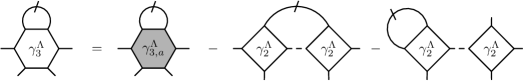
Figure 6: Diagrammatic structure of Eq. (78). The factors $\zeta^{\Lambda}$ appended at each leg of $\gamma_{3,a}^{\Lambda}$ are implicitly included in the diagram.

The last six terms on the right hand side of this equation can be seen diagrammatically as the possible distinct ways of connecting two out of the six external points of the quantity $\gamma_{2}^{\Lambda}\circ\bar{G}^{\Lambda}\circ\gamma_{2}^{\Lambda}$, and therefore acquire the same diagrammatic structure of the first two terms. Hence by performing a functional derivative with respect to $S^{\Lambda}$ we can finally write a relation between the three-particle vertex:

$$\gamma_{3}^{\Lambda}=\gamma^{\Lambda}_{3,a}\left[\zeta^{\Lambda},\zeta^{\Lambda},\zeta^{\Lambda},\bar{\zeta}^{\Lambda},\bar{\zeta}^{\Lambda},\bar{\zeta}^{\Lambda}\right]-\gamma^{\Lambda}_{2}\circ\bar{G}^{\Lambda}\circ\gamma^{\Lambda}_{2},$$ (79)

as depicted diagrammatically in Fig. 4. Let us also note explicitly that this equation is consistent with the fact that in the beginning of the flow the auxiliary 1PI three-particle vertex is equal to the amputated connected three particle Green’s function of the reference system.

As for the flow of the self energy one can see from Eq. (37), that no further diagrams appear by performing the flow in the auxiliary space, i.e., the self energy flow equation Eq. (26) remains the same, and the only differences arise indirectly due to the change of the vertex during the flow discussed above.

References

- Salmhofer (1999) M. Salmhofer, Renormalization: An Introduction (Theoretical and Mathematical Physics) (Springer, Berlin and Heidelberg, 1999), corrected ed., ISBN 9783540646662.
- Berges et al. (2002) J. Berges, N. Tetradis, and C. Wetterich, Phys. Rep. 363, 223 (2002).
- Kopietz et al. (2010) P. Kopietz, L. Bartosch, and F. Schütz, Introduction to the Functional Renormalization Group (Lecture Notes in Physics) (Springer, Berlin and Heidelberg, 2010), 1st ed., ISBN 9783642050930.
- Metzner et al. (2012) W. Metzner, M. Salmhofer, C. Honerkamp, V. Meden, and K. Schönhammer, Rev. Mod. Phys. 84, 299 (2012).
- Salmhofer (1998) M. Salmhofer, Communications in Mathematical Physics 194, 249 (1998).
- Salmhofer and Honerkamp (2001) M. Salmhofer and C. Honerkamp, Prog. Theor. Phys. 105, 1 (2001).
- Taranto et al. (2014) C. Taranto, S. Andergassen, J. Bauer, K. Held, A. Katanin, W. Metzner, G. Rohringer, and A. Toschi, Phys. Rev. Lett. 112, 196402 (2014).
- Kinza et al. (2013) M. Kinza, J. Ortloff, J. Bauer, and C. Honerkamp, Phys. Rev. B 87, 035111 (2013).
- Kinza and Honerkamp (2013) M. Kinza and C. Honerkamp, Phys. Rev. B 88, 195136 (2013).
- Rançon (2014) A. Rançon, Phys. Rev. B 89, 214418 (2014).
- Reuther and Thomale (2014) J. Reuther and R. Thomale, Phys. Rev. B 89, 024412 (2014).
- Rançon and Dupuis (2011a) A. Rançon and N. Dupuis, Phys. Rev. B 83, 172501 (2011a).
- Rançon and Dupuis (2011b) A. Rançon and N. Dupuis, Phys. Rev. B 84, 174513 (2011b).
- Rubtsov et al. (2008) A. N. Rubtsov, M. I. Katsnelson, and A. I. Lichtenstein, Phys. Rev. B 77, 033101 (2008).
- Brener et al. (2008) S. Brener, H. Hafermann, A. N. Rubtsov, M. I. Katsnelson, and A. I. Lichtenstein, Phys. Rev. B 77, 195105 (2008).
- Hafermann et al. (2008) H. Hafermann, S. Brener, A. N. Rubtsov, M. I. Katsnelson, and A. I. Lichtenstein, JETP Letters 86, 677 (2008).
- Rubtsov et al. (2009) A. N. Rubtsov, M. I. Katsnelson, A. I. Lichtenstein, and A. Georges, Phys. Rev. B 79, 045133 (2009).
- Yang et al. (2011) S.-X. Yang, H. Fotso, H. Hafermann, K.-M. Tam, J. Moreno, T. Pruschke, and M. Jarrell, Phys. Rev. B 84, 155106 (2011).
- Katanin (2013) A. A. Katanin, Journal of Physics A Mathematical General 46, 045002 (2013).
- Kirchner et al. (2013) S. Kirchner, F. Zamani, and E. Muñoz, arXiv:1301.3307 (2013).
- Muñoz et al. (2013) E. Muñoz, C. J. Bolech, and S. Kirchner, Phys. Rev. Lett. 110, 016601 (2013).
- Antipov et al. (2014) A. E. Antipov, E. Gull, and S. Kirchner, Phys. Rev. Lett. 112, 226401 (2014).
- Hague et al. (2004) J. P. Hague, M. Jarrell, and T. C. Schulthess, Phys. Rev. B 69, 165113 (2004).
- Toschi et al. (2007) A. Toschi, A. A. Katanin, and K. Held, Phys. Rev. B 75, 045118 (2007).
- Held et al. (2008) K. Held, A. A. Katanin, and T. A., Prog. Theor. Phys. Supplement 176, 117 (2008).
- Valli et al. (2010) A. Valli, G. Sangiovanni, O. Gunnarsson, A. Toschi, and K. Held, Phys. Rev. Lett. 104, 246402 (2010).
- Rohringer et al. (2013) G. Rohringer, A. Toschi, H. Hafermann, K. Held, V. I. Anisimov, and A. A. Katanin, Phys. Rev. B 88, 115112 (2013).
- Li (2014) G. Li, arXiv:1410.6861 (2014).
- Valli et al. (2014) A. Valli, T. Schäfer, P. Thunström, G. Rohringer, S. Andergassen, G. Sangiovanni, K. Held, and A. Toschi, arXiv:1410.4733 (2014).
- Pairault et al. (1998) S. Pairault, D. Sénéchal, and A.-M. S. Tremblay, Phys. Rev. Lett. 80, 5389 (1998).
- Hafermann et al. (2009) H. Hafermann, C. Jung, S. Brener, M. I. Katsnelson, A. N. Rubtsov, and A. I. Lichtenstein, Europhys. Lett. 85, 27007 (2009).
- Georges and Kotliar (1992) A. Georges and G. Kotliar, Phys. Rev. B 45, 6479 (1992).
- Georges et al. (1996) A. Georges, G. Kotliar, W. Krauth, and M. J. Rozenberg, Rev. Mod. Phys. 68, 13 (1996).
- Metzner and Vollhardt (1989) W. Metzner and D. Vollhardt, Phys. Rev. Lett. 62, 324 (1989).
- Hubbard (1963) J. Hubbard, Proc. R. Soc. A 276, 238 (1963).
- Kotliar et al. (2001) G. Kotliar, S. Y. Savrasov, G. Pálsson, and G. Biroli, Phys. Rev. Lett. 87, 186401 (2001).
- Hettler et al. (2000) M. H. Hettler, M. Mukherjee, M. Jarrell, and H. R. Krishnamurthy, Phys. Rev. B 61, 12739 (2000).
- Maier et al. (2005) T. Maier, M. Jarrell, T. Pruschke, and M. H. Hettler, Reviews of Modern Physics 77, 1027 (2005).
- Slezak et al. (2009) C. Slezak, M. Jarrell, T. Maier, and J. Deisz, Journal of Physics Condensed Matter 21, 435604 (2009).
- Rohringer et al. (2012) G. Rohringer, A. Valli, and A. Toschi, Phys. Rev. B 86, 125114 (2012).
- Hafermann (2014) H. Hafermann, Phys. Rev. B 89, 235128 (2014).
- Katanin (2004) A. A. Katanin, Phys. Rev. B 70, 115109 (2004).
- Eberlein (2014) A. Eberlein, Phys. Rev. B 90, 115125 (2014).
- Maier and Honerkamp (2012) S. A. Maier and C. Honerkamp, Phys. Rev. B 85, 064520 (2012).
- Katanin (2009) A. A. Katanin, Phys. Rev. B 79, 235119 (2009).
- Hafermann (2010) H. Hafermann, Numerical approaches to spatial correlations in strongly interacting fermion systems (Cuvillier, Göttingen, 2010), ISBN 9783869553474.
- Mandl and Shaw (2010) F. Mandl and G. Shaw, Quantum Field Theory (Wiley, Chichester, 2010), 2nd ed., ISBN 9780471496847.
- Schäfer et al. (2013) T. Schäfer, G. Rohringer, O. Gunnarsson, S. Ciuchi, G. Sangiovanni, and A. Toschi, Phys. Rev. Lett. 110, 246405 (2013).
- Janiš and Pokorný (2014) V. Janiš and V. Pokorný, Phys. Rev. B 90, 045143 (2014).