Entanglement-enhanced time-continuous quantum control in optomechanics

Abstract

The cavity-optomechanical radiation pressure interaction provides the means to create entanglement between a mechanical oscillator and an electromagnetic field interacting with it. Here we show how we can utilize this entanglement within the framework of time-continuous quantum control, in order to engineer the quantum state of the mechanical system. Specifically, we analyze how to prepare a low-entropy mechanical state by (measurement-based) feedback cooling operated in the blue detuned regime, the creation of bipartite mechanical entanglement via time-continuous entanglement swapping, and preparation of a squeezed mechanical state by time-continuous teleportation. The protocols presented here are feasible in optomechanical systems exhibiting a cooperativity larger than 1.

I Introduction

Quantum control plays a crucial role in modern quantum experiments across different fields. In optomechanics alone its applications range from feedback cooling of the mechanical motion Cohadon et al. (1999), mechanical squeezing Clerk et al. (2008); Woolley et al. (2008) and two-mode squeezing Woolley and Clerk (2013) to back-action elimination Wiseman (1995); Courty et al. (2003) with possible applictions in gravitational wave detection. Importantly for quantum information processing and communication, it can also be used to robustly generate entanglement between remote quantum systems, as has been demonstrated recently for spin qubits Dolde et al. (2014). At the same time entanglement itself can be an essential component to facilitate control of quantum systems, e. g., as a resource for teleportation Bennett et al. (1993) when employed as a means for remote state preparation. In optomechanics, pulsed entanglement between a mechanical oscillator and the electromagnetic field Hofer et al. (2011) has recently been demonstrated in an electromechanical setup Palomaki et al. (2013); state preparation (and verification) of an arbitrary mechanical quantum state (e. g., a Fock state) is yet to be accomplished (see, however, O’Connell et al. (2010)). Typical quantum control protocols are operated in a time-continuous fashion and often rely on continuous measurements which are capable of tracking the quantum state of the controlled system. The resulting measurement record—and the so-called conditional quantum state inferred from it—is then used as a basis for the applied feedback Wiseman and Milburn (2009). Thus, the control protocol’s success critically depends on the precision of the employed measurement. The most essential prerequisite for quantum limited feedback control turns out to be the regime of strong (linearized, thermal) cooperativity. This regime has been witnessed in several experiments in the past few years Murch et al. (2008); Teufel et al. (2011); Chan et al. (2011); Brooks et al. (2012); Safavi-Naeini et al. (2013); Purdy et al. (2013). Recently, monitoring a mechanical oscillator with a measurement strength matching its thermal decoherence rate (equivalent to a cooperativity above 1) and measurement-based feedback cooling to an occupation number of several phonons has been demonstrated in Wilson et al. (2014).

Figure 1: Different optomechanical setups considered in this article: (a) single homodyne detection for feedback cooling (non-unit efficiency is modeled by a beam-splitter before a perfect detector, marked by the yellow box; see Sec. III.1), (b) time-continuous teleportation, (c) time-continuous entanglement swapping, (d) detail of the entanglement swapping setup. The green (dark gray) dashed boxes mark the time-continuous Bell measurement setups, the orange (light gray) box in (d) marks the auxiliar stabilizing measurements.

In this article we explore protocols which exploit optomechanical entanglement as a resource for measurement-based time-continuous control of cavity-optomechanical systems (see Fig. 1 for the different setups being considered). The presented protocols rely on the fact that for a laser drive appropriately (blue) detuned from the cavity resonance, the radiation-pressure interaction generates entanglement between the mechanical oscillator and the cavity output light. We will show that due to this fact it is in principle possible to feedback-cool the mechanical motion to its ground state, even though the optomechanical interaction effects heating of the mechanical mode in this particular regime. This stands in contrast to common feedback-cooling schemes which operate on cavity resonance Cohadon et al. (1999); Wilson et al. (2014). The scheme presented here is based on standard homodyne detection to monitor a single quadrature of the output light, and feedback by (phase and amplitude) modulation of the driving laser. The feedback signal is calculated by applying linear–quadratic–Gaussian (LQG) control from classical control theory, which attains the optimal cooling performance for the chosen configuration. Beyond cooling, entanglement-based protocols for quantum control can be used to achieve more sophisticated quantum state engineering. We study in detail two optomechanical implementations of time-continuous Bell measurements Hofer et al. (2013): Time-continuous teleportation allows for preparation of a mechanical oscillator in a general Gaussian (squeezed) state, while time-continuous entanglement-swapping can be used to prepare two remote mechanical systems in an (Einstein–Podolsky–Rosen) entangled state. Both schemes generate dissipative dynamics which drive the mechanical system(s) into the desired stationary state. They are shown to work if the effective measurement strength is on the same order as the mechanical decoherence rate (i. e., for a optomechanical cooperativity of around 1), which is the same condition that holds for ground-state cooling Teufel et al. (2011); Chan et al. (2011), observation of back-action noise Murch et al. (2008); Purdy et al. (2013), and ponderomotive squeezing Brooks et al. (2012); Safavi-Naeini et al. (2013), all of which have been achieved experimentally. Although we here consider optomechanical systems only, the presented methods are very versatile, applicable to different (continuous and discrete) physical systems, and can be extended to describe more complex topologies, such as multiple interferometric measurements and quantum networks Hofer et al. (2013).

The results on time-continuous teleportation and entanglement swapping have been published in parts in Hofer et al. (2013). Here we provide an extended treatment focusing on an optomechanical implementation and present a detailed derivation of the resulting equations.

The manuscript is organized as follows: In Sec. II we summarize and illustrate the central results concerning cooling, mechanical squeezing, and bipartite mechanical entanglement generation. We start this section by discussing the phase diagram of the optomechanical steady state, emphasizing its unique features for blue detuned laser drive. Sec. III presents in detail all technical aspects in the derivation of our results. Some background information about quantum stochastic calculus and LQG control is presented in the appendices A and B.

II Central results

II.1 The cavity-optomechanical system

In this article we consider a cavity optomechanical system with a single mechanical mode oscillating at a resonance frequency $\omega_{m}$. The cavity has a resonance frequency $\omega_{c}$ and a [full width at half maximum (FWHM)] decay rate $\kappa$, and is driven by continuous-wave laser light at a frequency $\omega_{l}$. In a linearized description and in a frame rotating with $\omega_{l}$, the system is described by the effective Hamiltonian Aspelmeyer et al. (2014)

$$H_{\mathrm{sys}}=\omega_{m}c_{m}^{\dagger}c_{m}-\Delta_{l}c_{l}^{\dagger}c_{l}+g(c_{m}+c_{m}^{\dagger})(c_{l}+c_{l}^{\dagger}),$$ (1)

where $c_{m}$ and $c_{l}$ are bosonic annihilation operators of the mechanical and the optical mode respectively. $\Delta_{l}=\omega_{0}-\omega_{\mathrm{c}}$ is the detuning of the driving laser with respect to the cavity, and $g$ is the optomechanical coupling strength. In writing this Hamiltonian we implicitly assumed that the cavity is driven strongly, such that the radiation-pressure interaction can be linearized around a large classical intracavity amplitude. The coupling strength is then given by $g=g_{0}[2\kappa P/\hbar\omega_{0}(\kappa^{2}+\Delta^{2})]^{1/2}$ with the single-photon coupling $g_{0}$ and the input laser power $P$. To work with the linearized description we assume the existence of a unique classical steady state with a large intracavity photon number, thus neglecting effects of bistability Ghobadi et al. (2011); Aspelmeyer et al. (2014). Additionally we assume $g_{0}\ll\kappa,\omega_{m}$, which is needed to safely neglect nonlinear radiation pressure effects Aspelmeyer et al. (2014).

The linearized radiation-pressure Hamiltonian $H_{\mathrm{om}}=g(c_{m}+c_{m}^{\dagger})(c_{l}+c_{l}^{\dagger})$ can be decomposed into two terms: a beam-splitter like interaction $g(c_{m}c_{l}^{\dagger}+c_{m}^{\dagger}c_{l})$ which is resonant for $\Delta_{l}=-\omega_{m}$ (red detuned laser drive) and effects cooling of the mechanical motion, and a two-mode squeezing term $g(c_{m}c_{l}+c_{m}^{\dagger}c_{l}^{\dagger})$ which is dominant for $\Delta_{l}=\omega_{m}$ (blue driving) and is responsible for creation of optomechanical correlations and entanglement. For a resonant drive ($\Delta_{l}=0$) we retain the full Hamiltonian $\propto gx_{m}x_{l}$, which is commonly associated with quantum non-demolition (QND) measurements of harmonic oscillators Thorne et al. (1978); Braginsky et al. (1980) and is the interaction typically used for measurement-based feedback control of these systems Mancini et al. (1998); Doherty and Jacobs (1999); Hamerly and Mabuchi (2013). The optical and mechanical quadrature operators we define as $x_{i}=(c_{i}+c_{i}^{\dagger})/\sqrt{2}$ and $p_{i}=-\mathrm{i}(c_{i}-c_{i}^{\dagger})/\sqrt{2}$ ($i\in\left\{m,l\right\}$) which leads to canonical commutation relations $[x_{i},p_{j}]=\mathrm{i}\delta_{ij}$. In the following it will be convenient to collect them into the vector operator $\boldsymbol{X}=(x_{m},p_{m},x_{l},p_{l})^{\mathrm{T}}$.

II.2 The optomechanical phase diagram

Optomechanical sideband cooling and entanglement creation in steady state have been analyzed in detail in the literature Wilson-Rae et al. (2007); Marquardt et al. (2007); Genes et al. (2008a, b). Both phenomena are captured by the standard optomechanical master equation (MEQ) for the quantum state $\rho$, given by Wilson-Rae et al. (2007)

$$\begin{split}\dot{\rho}(t)&=\mathcal{L}\rho(t)=-\mathrm{i}[H,\rho(t)]+\kappa\mathcal{D}[c_{l}]\rho(t)\\ &\qquad+\gamma(\bar{n}+1)\mathcal{D}[c_{m}]\rho(t)+\gamma\bar{n}\mathcal{D}[c_{m}^{\dagger}]\rho(t)\end{split}$$ (2)

where $\mathcal{L}$ is the so-called Liouville operator. Here $\gamma$ denotes the (FWHM) width of the mechanical resonance, and $\bar{n}$ the mechanical bath’s mean phonon number. Optical and mechanical decoherence is described by the Lindblad operators $\mathcal{D}[c]\rho=c\rho c^{\dagger}-\tfrac{1}{2}\rho c^{\dagger}c-\tfrac{1}{2}c^{\dagger}c\rho$. As our system is Gaussian, its state is fully characterized by the first and second moments of $\boldsymbol{X}$, i. e., the mean values $\langle\boldsymbol{X}\rangle(t)=\mathrm{tr}[\boldsymbol{X}\rho(t)]$ and the symmetric covariance matrix

$$\mathbf{\Sigma}(t)=\operatorname{Re}\bigr{(}\langle\boldsymbol{X}\boldsymbol{X}^{\mathrm{T}}\rangle(t)\bigl{)}-\langle\boldsymbol{X}\rangle(t)\langle\boldsymbol{X}^{\mathrm{T}}\rangle(t).$$ (3)

(Throughout this paper we will often omit the explicit time argument for the sake of brevity if no ambiguity exists.) The linear equations of motion of $\langle\boldsymbol{X}\rangle$ and $\mathbf{\Sigma}$ are given by (App. B)

$$\frac{\operatorname{d}\!}{\operatorname{d}\!t}\langle\boldsymbol{X}\rangle(t) =\mathbf{F}\langle\boldsymbol{X}\rangle(t),$$ (4a)

$$\frac{\operatorname{d}\!}{\operatorname{d}\!t}\mathbf{\Sigma}(t) =\mathbf{F}\mathbf{\Sigma}(t)+\mathbf{\Sigma}(t)\mathbf{F}^{\mathrm{T}}+\mathbf{N}.$$ (4b)

The $4\times 4$ matrices $\mathbf{F}$ and $\mathbf{N}$ describe the system’s dynamics and noise properties respectively, and are algebraically connected to the Liouvillian in the MEQ (2).

Provided the system is stable, it will in the long-term assume a steady state, $\lim_{t\rightarrow\infty}\rho(t)=\rho^{\mathrm{ss}}$, where $\rho^{\mathrm{ss}}$ is determined by the condition $\mathcal{L}\rho^{\mathrm{ss}}=0$. The stability of a linear system can be assessed by applying the Routh–Hurwitz (RH) stability criterion I.S. Gradshteyn and I.M. Ryshik (2007) which is fulfilled iff all eigenvalues of $\mathbf{F}$ have negative real parts. If a stable steady state exists the means $\langle\boldsymbol{X}\rangle^{\mathrm{ss}}{:=}\mathrm{tr}[\boldsymbol{X}\rho^{\mathrm{ss}}]=0$ will vanish, while the steady-state covariance matrix $\mathbf{\Sigma}^{\mathrm{ss}}$ is given by the solution to the so-called Lyapunov equation, which is obtained from (4b) by setting its left-hand side to zero, i. e., $\mathbf{F}\mathbf{\Sigma}^{\mathrm{ss}}+\mathbf{\Sigma}^{\mathrm{ss}}\mathbf{F}^{\mathrm{T}}+\mathbf{N}=0$. This equation can readily be solved to obtain steady-state properties such as the mean mechanical occupation number $n_{m}^{\mathrm{ss}}=\langle c_{m}^{\dagger}c_{m}\rangle^{\mathrm{ss}}$ or logarithmic negativity $E_{\mathcal{N}}^{\mathrm{ss}}$ Vidal and Werner (2002); Plenio (2005). In this section we will mainly be concerned with these steady-state properties of optomechanical systems.

The characteristic features of an optomechanical system’s steady state can nicely be illustrated by plotting a phase diagram with respect to the laser detuning $\Delta_{l}$ and the optomechanical coupling $g$, as depicted in Fig. 2 for an optomechanical system in the resolved sideband regime ($\kappa<\omega_{m}$) for a high-Q ($Q=\omega_{m}/\gamma$) mechanical oscillator. The grey background depicts the regions of instability, given by the corresponding Routh–Hurwitz criterion, where no steady state exists. The first thing to note is that the system is unstable in nearly all the right half-plane, i. e., for blue detuned laser drive, while for red detuning the system becomes unstable only for appreciably high optomechanical coupling. Centered around the first mechanical sideband at $\Delta_{l}=-\omega_{m}$ where the beam-splitter part of the optomechanical interaction is resonant, lies the region where $n_{m}^{\mathrm{ss}}<1$ (dashed purple line) and thus ground-state cooling is possible. Right at the border of stability, for a similar detuning, we find regions of large steady-state entanglement between the intracavity field and the mechanical resonator (colored in turquoise/blue) Genes et al. (2008b). On the opposite side of the phase diagram, around the blue mechanical sideband at $\Delta_{l}=\omega_{m}$, we also expect to observe optomechanical entanglement due to the effect of the optomechanical two-mode squeezing dynamics. However, there the formation of a steady state is inhibited by the optomechanical instability which is due to parametric amplification of the amplitude of both the mechanical and the optical mode Aspelmeyer et al. (2014). The connection of laser cooling, entanglement generation, and the instability region has been analyzed in detail in Genes et al. (2008b).

(a)

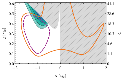
(b)

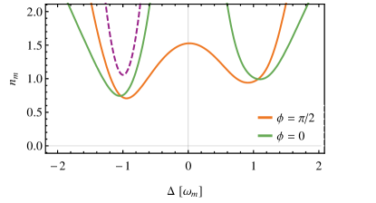
Figure 2: (Color online) Upper plot: Steady-state phase diagram of an optomechanical system for $\kappa=\omega_{m}/2$, $Q=5\cdot 10^{6}$, $\bar{n}=3.5\cdot 10^{5}$. The gray hatched area depicts unstable regions where no steady-state exists. The dashed purple (dark gray) line shows regions of ground state cooling of the mechanical oscillator, here $n_{m}^{\mathrm{ss}}<1$. The turquoise/blue (gray unhatched) area shows optomechanical entanglement (logarithmic negativity $E_{\mathcal{N}}^{\mathrm{ss}}$), with largest values close to the instability region. The orange (light gray) line encloses the regions where the conditional mean mechanical occupation number $\langle c^{\dagger}_{m}c_{m}\rangle_{c}^{\mathrm{ss}}<1$ for a measurement of the optical phase quadrature, i. e., $\phi=\pi/2$. The right axis shows the corresponding optomechanical cooperativity, given by $C=4g^{2}/(\bar{n}+1)\gamma\kappa$. Lower Plot: Cut through the phase diagram at $g=\omega_{m}/10$, depicting the conditional phonon number $\langle c^{\dagger}_{m}c_{m}\rangle_{c}^{\mathrm{ss}}$ for LO phases $\phi=\pi/2$ (orange [light gray] line) and $\phi=0$ (green [dark gray] line). The dashed purple line again shows the mean occupation number for the unconditional state for sideband cooling.

Although no steady state exists for a blue-detuned laser drive, various alternative approaches permit to work with the resonantly enhanced two-mode squeezing dynamics of the optomechanical interaction. Pulsed optomechanical entanglement creation, for example,—which does not require to be operated in a stable regime—has been analyzed in detail in Hofer et al. (2011), and has been experimentally demonstrated (for an electromechanical system) in Palomaki et al. (2013). Working with a continuous-wave blue-detuned laser drive on the other hand, is still possible if we employ stabilizing feedback which inhibits the exponential growth of the optomechanical system’s quadratures. One possible type of feedback is measurement-based feedback using homodyne detection, which we will consider in the following.

By adding a homodyne detector to our setup [measuring a single light quadrature defined by the local oscillator (LO) angle $\phi$], we can condition the optomechanical system’s state on the resulting photo-current $I(t)$, which leads to a stochastic master equation (SME) in the Itō sense (see Gardiner and Zoller (2004); Wiseman and Milburn (2009) and Sec. III.1)

$$\operatorname{d}\!\rho_{c}(t)=\mathcal{L}\rho_{c}(t)\operatorname{d}\!t+\sqrt{\eta\kappa}\,\mathcal{H}[\mathrm{e}^{\mathrm{i}\phi}c_{l}]\rho_{c}(t)\operatorname{d}\!W(t).$$ (5)

$\rho_{c}$ is the so-called conditional quantum state, which describes our knowledge of the system given a specific measurement record $I(t)$. The effect of conditioning is described by the operator $\mathcal{H}[s]\rho_{c}=(s-\mathrm{tr}[s\rho_{c}])\rho_{c}+\rho_{c}(s-\mathrm{tr}[s\rho_{c}])^{\dagger}$. $\mathcal{H}$ is thus nonlinear in $\rho_{c}$, as is expected for a measurement term. $I(t)$ can be expressed as

$$I(t)\operatorname{d}\!t=\sqrt{\eta\kappa}\langle c_{l}\mathrm{e}^{-\mathrm{i}\phi}+c_{l}^{\dagger}\mathrm{e}^{\mathrm{i}\phi}\rangle_{c}(t)\operatorname{d}\!t+\operatorname{d}\!W(t),$$ (6)

where $\operatorname{d}\!W$ is a Wiener increment with $\operatorname{d}\!W(t)^{2}=\operatorname{d}\!t$, and $0<\eta<1$ is the efficiency of the detection. Here and in the following we denote by $\langle A\rangle_{c}(t)=\mathrm{tr}[A\rho_{c}(t)]$ the expectation value with respect to the conditional state. In contrast to the conditional state $\rho_{c}$ which solves a SME, we will call the solution of a standard MEQ [such as (2)] the unconditional state, which we denote by $\rho$.

Gaussian conditional quantum states are fully described by the mean vector $\boldsymbol{\hat{X}}(t)=\langle\boldsymbol{X}\rangle_{c}(t)$ and covariance matrix

$$\mathbf{\hat{\Sigma}}(t)=\operatorname{Re}\bigr{(}\langle\boldsymbol{X}\boldsymbol{X}^{\mathrm{T}}\rangle_{c}(t)\bigl{)}-\langle\boldsymbol{X}\rangle_{c}(t)\langle\boldsymbol{X}^{\mathrm{T}}\rangle_{c}(t),$$ (7)

defined with respect to $\rho_{c}$. Their equations of motion are given by a linear stochastic differential equation and a (deterministic) matrix Riccati equation respectively,

$$\operatorname{d}\!\boldsymbol{\hat{X}}(t) =\mathbf{F}\boldsymbol{\hat{X}}(t)\operatorname{d}\!t+\mathbf{K}(t)\bigl{[}I(t)-\mathbf{H}\boldsymbol{\hat{X}}(t)\bigr{]}\operatorname{d}\!t,$$ (8)

$$\frac{\operatorname{d}\!}{\operatorname{d}\!t}{\mathbf{\hat{\Sigma}}(t)} =\mathbf{F}\mathbf{\hat{\Sigma}}(t)+\mathbf{\hat{\Sigma}}(t)\mathbf{F}^{\mathrm{T}}+\mathbf{N}$$

$$\qquad-\big{[}\mathbf{\hat{\Sigma}}(t)\mathbf{H}^{\mathrm{T}}+\mathbf{M}\big{]}\big{[}\mathbf{\hat{\Sigma}}(t)\mathbf{H}^{\mathrm{T}}+\mathbf{M}\big{]}^{\mathrm{T}},$$ (9)

where $\mathbf{H}$ describes the homodyne measurement and $\mathbf{M}$ is related to the system’s noise properties (see App. B). $\mathbf{K}(t)$ is a time-dependent gain factor which depends on $\mathbf{\hat{\Sigma}}(t)$. For a one-dimensional system [with a two-dimensional phase space $(x,p)$] these equations allow us to give a simple graphic interpretation of the SME (5) in terms of a phase-space description (see Fig. 3): The conditional trajectory $\boldsymbol{\hat{X}}$ (blue line) is determined by the measurements $I(t)$ and therefore follows a random walk in phase space. The covariance matrix $\mathbf{\hat{\Sigma}}$ (turquoise ellipse) on the other hand evolves deterministically, independent of the measurement results. Averaging over all possible phase-space trajectories recovers the broad Gaussian distribution described by the standard MEQ (2) [or equivalently, equations (4)]. For an unstable system (e. g., in the blue detuned regime), the blue line will spiral outwards, leading to a growing unconditional covariance. The conditional covariance matrix $\mathbf{\hat{\Sigma}}$, however, may still possess a (finite) steady state. This is due to the fact that the exponential growth is tracked by the conditional mean, with respect to which the covariance matrix is defined. The steady-state conditional covariance matrix $\mathbf{\hat{\Sigma}}^{\mathrm{ss}}$ can be found in analogy to $\mathbf{\Sigma}^{\mathrm{ss}}$ by setting the left-hand side of equation (II.2) to zero and by solving the resulting algebraic Riccati equation Wiseman and Milburn (2009).

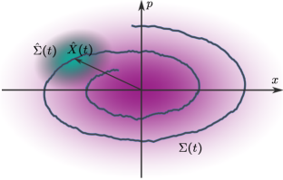
Figure 3: (Color online) Schematic comparison of the master equation (2) and the stochastic master equation (5) for a single mode Gaussian system in phase space. The conditional state with a covariance $\mathbf{\hat{\Sigma}}(t)$, depicted by the turquoise (small, off-centered) elipse, moves through phase space on a trajectory given by a realisation of $\boldsymbol{\hat{X}}(t)$ (blue [dark gray] line). Averaging over many sample paths recovers the broad, unconditional distribution, determined by $\mathbf{\Sigma}(t)$ (purple [large, centered] ellipse).

Having obtained $\mathbf{\hat{\Sigma}}^{\mathrm{ss}}$ we can easily evaluate the conditional state’s mean mechanical occupation number, depicted in Fig. 2(a) for a measurement of the phase quadrature of the light field, i. e., $\phi=\pi/2$. We find a large region where $\langle c^{\dagger}_{m}c_{m}\rangle_{c}^{\mathrm{ss}}<0.4$ for all detunings $-\omega_{m}\lesssim\Delta_{l}\lesssim\omega_{m}$ (orange line). In the region around the red sideband $\Delta_{l}\approx-\omega_{m}$ this effect can mainly be attributed to passive sideband cooling of the mirror, which we discussed above. However, we now also find a region of low occupation on the opposite (blue) sideband at $\Delta_{l}\approx\omega_{m}$. In this region the reduction of the conditional phonon number, which at the same time means an increase of the mechanical state’s purity, is due to correlations between the mechanical oscillator and the light field. These correlations allow us to extract information about the mechanics from the homodyne measurement. We will see in the next section that in the sideband-resolved regime $\kappa<\omega_{m}$ this effect is strongest for $\Delta_{l}\approx\omega_{m}$ where the two-mode squeezing, entangling term of the optomechanical Hamiltonian is resonant.

To illustrate how the choice of the LO phase influences the conditional mechanical occupation we plot a cut through Fig. 2(a) at a fixed optomechanical coupling $g=\omega_{m}/20$ in Fig. 2(b). If we choose to measure the optical amplitude quadrature we find that on resonance we do not have a reduction of the conditional phonon number. For a detuned laser drive ($|\Delta_{l}|\gtrsim\omega_{m}$) however, we again find regions of $\langle c^{\dagger}_{m}c_{m}\rangle_{c}^{\mathrm{ss}}<1$. This is easily explained by noting that on resonance ($\Delta_{l}=0$) only the optical phase quadrature couples to the mechanical oscillator, while the amplitude quadrature contains noise only. Measuring the amplitude quadrature therefore does not allow us to make inferences about the mechanical motion. In general there will be an optimal LO angle, depending on all system parameters (especially $g$, $\Delta_{l}$, $\kappa$) at which we obtain maximal information about the mechanical motion. Thus, homodyne detection at this particular angle yields the minimal conditional occupation. Typically—especially in the weak-coupling regime where $g<\kappa$—the optimal angle corresponds to the optical quadrature which is anti-squeezed by the optomechanical interaction and thus features the best signal-to-noise ratio. We will see in the next section how these features of the optomechanical phase diagram connect to feedback cooling of the mechanical oscillator.

II.3 Optomechanical Feedback Cooling

Now that we discussed the conditional optomechanical state in detail, the question arises whether it can be realized via feedback, i. e., whether we can prepare the unconditional state of the system such that it resembles the conditional state.

Consider the setup depicted in Fig. 1(a), where the results from a homodyne measurement of the cavity output light are fed back to the optomechanical system in a suitable manner, such that the mechanical system is driven to a low entropy steady state. This situation has been analyzed in Mancini et al. (1998); Doherty and Jacobs (1999); Genes et al. (2008a); Hamerly and Mabuchi (2013). However, the regime discussed for feedback cooling is typically restricted to resonant drive and the bad-cavity regime $\kappa>\omega_{m}$. In this section we will discuss that feedback cooling can also be effectively operated in the sideband-resolved regime $\kappa<\omega_{m}$, and even on the blue sideband $\Delta_{l}=\omega_{m}$, which is normally affiliated with heating. Here we will show that we can harness the entanglement created by the optomechanical two-mode squeezing interaction for a measurement-based feedback scheme, which enables us to cool the mechanical motion to its ground state.

Feedback onto the mechanical system can either be effected by direct driving through a piezoelectric device Poggio et al. (2007), or by modulation of the laser input, as we will assume in the following. This type of optical feedback can be described by adding an additional time-dependent term

$$H_{\mathrm{fb}}=-\mathrm{i}\sqrt{\kappa}[\varepsilon(t)^{*}c_{l}-\varepsilon(t)c_{l}^{\dagger}]=\sqrt{2\kappa}[u_{p}(t)x_{l}+u_{x}(t)p_{l}]$$ (10)

to the Hamiltonian, where $\varepsilon(t)=u_{x}(t)+\mathrm{i}u_{p}(t)\in\mathbb{C}$ is the complex amplitude of the feedback signal, and $|\varepsilon(t)|^{2}$ accordingly is the incoming photon flux. To choose an appropriate feedback strategy we employ quantum linear quadratic Gaussian (LQG) control Belavkin (1999), which is designed to minimize a quadratic cost function as described in App. B. Applied to feedback cooling the basic working principle is the following: From the measurement results of the homodyne detection we calculate the system’s conditional state $\rho_{c}(t)$, whose evolution is described by (5). Based on this state we can then determine the optimal feedback signal $\varepsilon(t)$ which minimizes the steady-state mechanical occupation number $\langle c_{m}^{\dagger}c_{m}\rangle^{\mathrm{ss}}=\tfrac{1}{2}[\langle x_{m}^{2}+p_{m}^{2}\rangle^{\mathrm{ss}}-1]$. This of course means that the final occupation number depends on the conditional state (more specifically on the covariance matrix $\hat{\mathbf{\Sigma}}$), and thus on the chosen LO angle for the homodyne detection as we discussed above. A suitable cost function for this problem is given by

$$h(x_{m}(t),p_{m}(t),\varepsilon(t))=h_{m}\left[x_{m}(t)^{2}+p_{m}(t)^{2}\right]+|\varepsilon(t)|^{2},$$ (11)

with $h_{m}>0$. Note that $h$ also includes a contribution by the feedback signal $\varepsilon$, which precludes feedback strategies with unrealistically high feedback strength. The parameter $h_{m}$ therefore effects a trade-off between feedback strength and final occupation number $n_{m}^{\mathrm{ss}}$: high values of $h_{m}$ result in low occupation number possibly requiring large $|\varepsilon|$ and vice versa. The mean photon flux in the feedback signal can be calculated as described in App. B. For the parameters used in this section we find that on average $|\varepsilon|^{2}$ is small compared to the overall driving strength in typical experiments. Only in the region of $\kappa\rightarrow 0$—where almost no photons enter the cavity—the required $|\varepsilon|^{2}$ may increase dramatically. We note that in order for LQG control to work correctly, certain observability and controllability conditions need to be satisfied Wiseman and Milburn (2009), which is indeed the case for our system. Additionally, we assume here that the feedback is instantaneous. In practice this means that any feedback delay $\tau$ should be small on the typical timescales of the system, i. e., $\tau\ll 1/\omega_{m},\ 1/\kappa$.

(a)

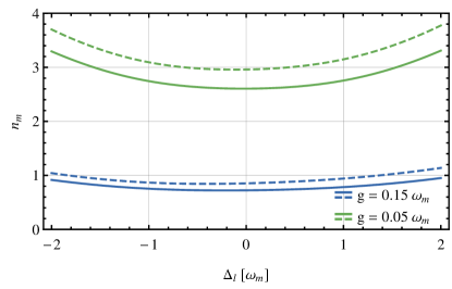
(b)

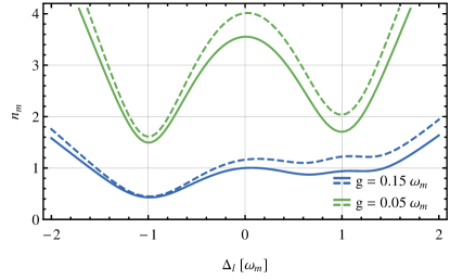
Figure 4: (Color online) Steady-state mechanical occupation number $n_{m}^{\mathrm{ss}}$ minimized with respect to the LO angle $\phi$ against detuning of the driving laser $\Delta_{l}$ (a) in the bad-cavity regime ($\kappa=4\omega_{m}$) and (b) in the sideband-resolved regime ($\kappa=\omega_{m}/2$), for detection efficiencies $\eta=1$ (solid lines) and $\eta=8/10$ (dashed lines). Different colors/gray levels denote different coupling strengths $g$. Other parameters: $Q=5\cdot 10^{6}$, $\bar{n}=3.5\cdot 10^{5}$, $h_{m}=100$

The final mechanical occupation is found by first calculating the steady-state variances $(\Delta x_{m})^{2}$ and $(\Delta p_{m})^{2}$ for a closed feedback loop as outlined in App. B. $n_{m}^{\mathrm{ss}}$ is then given by $n_{m}^{\mathrm{ss}}=\tfrac{1}{2}[(\Delta x_{m})^{2}+(\Delta p_{m})^{2}-1]$ (for $\langle x_{m}\rangle^{\mathrm{ss}}=\langle p_{m}\rangle^{\mathrm{ss}}=0$).

In Fig. 4 we plot the steady-state occupation numbers of the feedback-cooled mechanical mode against the laser detuning $\Delta_{l}$, for the bad-cavity regime (upper plot) and the sideband-resolved regime (lower plot), for two different coupling strengths $g$. For each detuning the homodyne phase $\phi$ is chosen such, that the occupation number is minimized. Note that we keep $g$ constant while varying $\Delta_{l}$ (or $\kappa$). This means that the driving laser power has to be adjusted accordingly. In the bad-cavity regime $\kappa>\omega_{m}$ we find that driving on resonance is favorable for both values of $g$. In this case the optimal LO phase is $\phi=\pi/2$, as discussed in the previous section. This is the usual regime for feedback cooling Cohadon et al. (1999); Wilson et al. (2014), which is inspired by the idea of quantum non-demolition measurements Braginsky and Khalili (1996), as they are commonly used in gravitational wave detection.

For micro-mechanical systems, however, the sideband-resolved regime $\kappa<\omega_{m}$ is typically more relevant. In this regime the picture changes completely. For weak coupling ($g<\kappa$) we find two pronounced dips at both mechanical sidebands ($\Delta_{l}=\pm\omega_{m}$), where $n_{m}^{\mathrm{ss}}$ is locally minimal and clearly lies below the value on resonance. It is obvious from the figure that cooling works best on the red sideband ($\Delta_{l}=-\omega_{m}$), where we have a cumulative effect from passive sideband and feedback cooling (see also Fig. 5). However, even on the blue sideband ($\Delta_{l}=\omega_{m}$)—which is commonly associated with heating—we find an appreciable reduction of the mechanical occupation by feedback cooling. As we discussed in the previous section, we can attribute this effect to large optomechanical correlations, which allow for a good read out of the mechanical motion and thus a good feedback performance. If we increase the coupling strength to $g=0.3\kappa$ we see a peak appearing around the blue sideband (which we attribute to ponderomotive squeezing of the output fields), pushing the occupation number above the value at $\Delta_{l}=0$. For both regimes we plot graphs for two different detection efficiencies $\eta=1$ (lossless detection) and $\eta=8/10$. Clearly, non-unit detection efficiency leads to a noticeable degradation of feedback-cooling performance. Only at the red sideband and in the sideband-resolved regime, where the effect of sideband cooling dominates, the final occupation number is virtually unaffected.

Figure 5(a) shows the mechanical occupation for three detunings $\Delta_{l}=0,\pm\omega_{m}$ plotted against $g$. For $\Delta_{l}=-\omega_{m}$ we show, additionally to the closed-loop feedback solution (red solid line), the solution for sideband cooling (red dashed line). While for $\Delta_{l}=0$ and $\Delta_{l}=-\omega_{m}$ the occupation number steadily decreases—in the depicted range—for growing $g$, for $\Delta_{l}=\omega_{m}$ a clear minimum is visible in the weak coupling regime at $g\approx\kappa/10$. This minimum lies well below the value for $\Delta_{l}=0$ (but still above the value for the red sideband). This means that there exists a considerably large parameter regime where a detuned operation significantly improves the performance of feedback cooling. Note that all curves rise drastically in the strong-coupling regime, where $g/\kappa\gtrsim 1$ (not shown in the plot). In Fig. 5(b) we plot $n_{m}^{\mathrm{ss}}$ against cavity linewidth $\kappa$ for constant coupling $g$. Again we find that feedback on the sidebands works best in the sideband-resolved regime, while in the bad cavity regime working on resonance yields (slightly) better performance. Again, the occupation number is minimized with respect to the homodyne phase $\phi$ at each point in the plot.

(a)

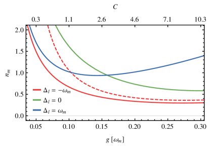
(b)

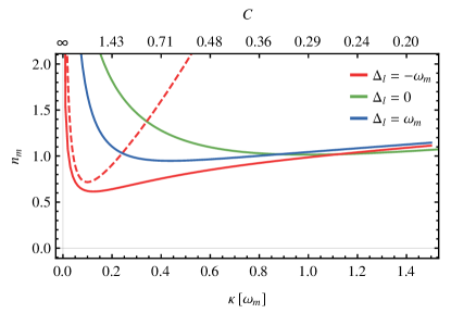
Figure 5: (Color online) Steady-state mechanical occupation number $n_{m}^{\mathrm{ss}}$ minimized with respect to $\phi$ for different driving frequencies $\Delta_{l}=0,\pm\omega_{m}$, corresponding to a laser drive on the mechanical sidebands and on resonance (represented by different colors/gray levels). Solid lines represent feedback cooling, while the dashed line (for $\Delta_{l}=-\omega_{m}$ only) corresponds to sideband cooling without feedback. (a) $n_{m}^{\mathrm{ss}}$ against coupling $g$ for fixed cavity decay rate $\kappa=\omega_{m}/2$ (sideband resolved regime). (b) $n_{m}^{\mathrm{ss}}$ against $\kappa$ for $g=\omega_{m}/10$ (weak coupling regime). Other parameters for both (a) and (b): $Q=5\cdot 10^{6}$, $\bar{n}=3.5\cdot 10^{5}$, $h_{m}=100$, $\eta=1$

In summary we illustrated that feedback cooling in the resolved-sideband regime is a viable option for cooling the mechanical oscillator into its ground state. It turns out that in this regime driving the system on the blue mechanical sideband yields a lower mechanical occupation number than operating on resonance. As an extension of this protocol we will show in the next section, that a similar setup operating at the same working point can be used to remotely prepare a squeezed mechanical state via time-continuous teleportation.

II.4 Time-continuous optomechanical teleportation

Time-continuous teleportation is facilitated by what we call a time-continuous Bell measurement Hofer et al. (2013), as depicted in Fig. 1(b): The output field $A$ of an optomechanical system (denoted by $S$) is mixed with a second field $B$ on a beam-splitter. The resulting fields are then sent to two homodyne detection setups which measure the Einstein–Podolsky–Rosen (EPR) quadratures $x_{+}=x_{a}+x_{b}$ and $p_{-}=p_{a}-p_{b}$ where $x_{a}$, $x_{b}$ and $p_{a}$, $p_{b}$ are the amplitude and phase quadratures of the respective fields. The field $B$ is prepared in a pure state of Gaussian squeezed white noise, which we denote by $|M\rangle$, where $M\in\mathds{C}$ characterizes the squeezing (see App. C); $|M|$ describes the absolute increase/reduction of the anti-/squeezed quadrature, while $\arg{(M)}$ determines the squeezing angle. Provided the optomechanical system–field interaction creates entanglement between the mechanical mode and the outgoing light field, the state of $B$ can be teleported to the mechanical oscillator by applying (instantaneous) feedback proportional to the measurement results of the Bell measurement ($I_{\pm}$). This effectively generates dissipative dynamics which drive the mechanical system into a steady state coinciding with the input light state. In Sec. III.2 we derive the constitutive equations of motion (the conditional master equation and feedback master equation) for a generic system. In this section we will focus on the optomechanical implementation. Technical details are discussed in Sec. III.4.1.

In order to successfully implement continuous teleportation in optomechanical systems we need to appropriately design our measurement setup. To do this we first need a clear picture of the system’s dynamics: In the regime $g\ll\kappa\ll\omega_{m}$ and for a blue drive with $\Delta_{l}=\omega_{m}$ the optomechanical interaction is $H_{\mathrm{om}}\approx g(c_{m}c_{l}+c_{m}^{\dagger}c_{l}^{\dagger})$. Under the weak-coupling condition ($g\ll\kappa$) the cavity follows the mechanical mode adiabatically. We will see that in this regime we effectively obtain the required entangling interaction between the mirror and the outgoing field. Moreover, the mechanical oscillator resonantly scatters photons into the lower sideband at $\omega_{\mathrm{c}}=\omega_{0}-\omega_{m}$. Spectrally, the photons which are correlated with the mechanical motion are therefore located at this sideband frequency. We thus set up our Bell measurement in the following way: Firstly, we choose the center frequency of the squeezed input light located at the sideband frequency $\omega_{\mathrm{c}}$. Secondly, we now use heterodyne detection to measure quadratures at the same frequency.

In Sec. III.4.1 we show that after adiabatic elimination of the cavity mode and a rotating-wave approximation, the evolution of the conditional mechanical state $\rho_{c}^{(m)}$ in a rotating frame with $\omega_{m}$ (neglecting the mechanical frequency shift by the optical-spring effect, see Sec. III.4.1) is described by the SME

$$\operatorname{d}\!\rho^{(m)}_{c}=\gamma_{-}\mathcal{D}[c_{m}]\rho^{(m)}_{c}\operatorname{d}\!t+\gamma_{+}\mathcal{D}[c_{m}^{\dagger}]\rho^{(m)}_{c}\operatorname{d}\!t\\ -\sqrt{\frac{\eta g^{2}\kappa}{2}}\left\{\mathcal{H}[\mathrm{i}\mu\eta_{+}c_{m}^{\dagger}]\rho^{(m)}_{c}\operatorname{d}\!W_{+}-\mathcal{H}[\nu\eta_{+}c_{m}^{\dagger}]\rho^{(m)}_{c}\operatorname{d}\!W_{-}\right\},$$ (12)

where we defined $\gamma_{-}=\gamma(\bar{n}+1)+2g^{2}\mathrm{Re}(\eta_{-})$, $\gamma_{+}=\gamma\bar{n}+2g^{2}\mathrm{Re}(\eta_{+})$ and $\eta_{\pm}=[\kappa/2+\mathrm{i}(-\Delta_{l}\pm\omega_{m})]^{-1}$. The second row describes passive cooling and heating effects via the optomechanical interaction, as has been derived before in the quantum theory of sideband cooling Wilson-Rae et al. (2007); Marquardt et al. (2007). The third row describes the time-continuous Bell measurement, where the squeezing parameter $M$ is encoded in $\mu=1-\alpha$ and $\nu=1+\alpha$, with $\alpha=(N+M)/(N+M^{*}+1)$ (App. C). The parameter $N>0$ is connected to $M$ via $|M|^{2}=N(N+1)$. $\eta$ is the detection efficiency as before. The measured photo-currents of the Bell measurement are

$$I_{+}\operatorname{d}\!t =-\mathrm{i}\sqrt{\eta g^{2}\kappa/2}\,\langle\eta_{+}c_{m}^{\dagger}-\mathrm{H.\,c.}{}\rangle\operatorname{d}\!t+\operatorname{d}\!W_{+},$$ (13a)

$$I_{-}\operatorname{d}\!t =\sqrt{\eta g^{2}\kappa/2}\,\langle\eta_{+}c_{m}^{\dagger}+\mathrm{H.\,c.}{}\rangle\operatorname{d}\!t+\operatorname{d}\!W_{-},$$ (13b)

where $\operatorname{d}\!W_{\pm}$ are correlated Wiener increments whose (co-)variances are given by

$$w_{1}\operatorname{d}\!t {:=}(\operatorname{d}\!W_{+})^{2}=[N+1+(M+M^{*})/2]\operatorname{d}\!t,$$ (14a)

$$w_{2}\operatorname{d}\!t {:=}(\operatorname{d}\!W_{-})^{2}=[N+1-(M+M^{*})/2]\operatorname{d}\!t,$$ (14b)

$$w_{3}\operatorname{d}\!t {:=}\operatorname{d}\!W_{+}\operatorname{d}\!W_{-}=-[\mathrm{i}(M-M^{*})/2]\operatorname{d}\!t,$$ (14c)

as is shown in Sec. III.2. For the choice $\Delta_{l}=\omega_{m}$ we have $\eta_{+}=2/\kappa$ and $\eta_{-}=1/(\tfrac{\kappa}{2}+2\mathrm{i}\omega_{m})$. Thus $I_{\pm}$ approximately correspond to measurements of the mechanical quadratures $p_{m}$ and $x_{m}$ respectively. We model the feedback as instantaneous displacements of the mechanical oscillator in phase space, where the feedback strength is proportional to the heterodyne currents $I_{\pm}(t)$. This is described by Hamiltonian terms $I_{\pm}(t)F_{\pm}$, where $F_{\pm}=F_{\pm}^{\dagger}$ are generalized forces. The feedback operators we choose to be $F_{+}=-\sqrt{2g^{2}\kappa}\,\eta_{+}\,x_{m}$ and $F_{-}=-\sqrt{2g^{2}\kappa}\,\eta_{+}\,p_{m}$, which generate a displacement in $p_{m}$ and $x_{m}$ respectively. The prefactors of $F_{\pm}$ (i. e., the feedback gain) we chose such that they match the measurement strength of the Bell detection. The corresponding feedback master equation (in the same rotating frame) can be written as

$$\dot{\rho}^{(m)}=\gamma(\bar{n}+1)\mathcal{D}[c_{m}]\rho^{(m)}+\gamma\bar{n}\mathcal{D}[c_{m}^{\dagger}]\rho^{(m)}\\ +(4g^{2}/\kappa)\left\{\lambda_{1}(\epsilon)\mathcal{D}[J_{1}(\epsilon)]+\lambda_{2}(\epsilon)\mathcal{D}[J_{2}(\epsilon)]\right\}\rho^{(m)},$$ (15)

where $\epsilon=[1+(4\omega_{m}/\kappa)^{2}]^{-1}$ quantifies the suppression of the counter-rotating interaction terms (i. e., the optomechanical beam-splitter). This suppression is large ($\epsilon\ll 1$) in the sideband-resolved regime where $\kappa\ll\omega_{m}$ and small ($\epsilon\approx 1$) in the bad-cavity regime ($\kappa\gtrsim\omega_{m}$). The effective Lindblad terms are determined by $\lambda_{i}$ and $J_{i}$, which are obtained (see App. D) from the eigenvalue decomposition of the positive matrix

$$\Lambda=\begin{pmatrix}\frac{w_{2}}{\eta}-\frac{1}{2}(1+\epsilon)&-\frac{w_{3}}{\eta}+\frac{\mathrm{i}}{2}(1+\epsilon)\\ -\frac{w_{3}}{\eta}-\frac{\mathrm{i}}{2}(1+\epsilon)&\frac{w_{1}}{\eta}-\frac{1}{2}(1+\epsilon)\end{pmatrix}.$$

For efficient detection ($\eta=1$) we obtain $\lambda_{1}=(2N+1)+O(\epsilon)$ and $\lambda_{2}=O(\epsilon)$, which means that in the sideband-resolved regime the jump operator $J_{2}(\epsilon)$ contributes only weakly. In zeroth order in $\epsilon$ the dominating dissipative dynamics are generated by $J_{1}(0)\propto-\mathrm{i}(2N+1-M-M^{*})x_{m}+(1+M-M^{*})p_{m}$. If we define as $U_{\pi/2}$ the local unitary which effects the canonical transformation $x_{m}\rightarrow p_{m}$, $p_{m}\rightarrow-x_{m}$, we find by comparison with (89) that $U_{\pi/2}^{\dagger}J_{1}(0)U_{\pi/2}|-M\rangle=0$. Taking into account relations (88) one can easily show that $U_{\pi/2}{|-M\rangle}=|M\rangle$. This means that $|M\rangle\langle M|$ is a dark state of $D[J_{1}(0)]$ and thus in the ideal limit of $\gamma=0$, $\epsilon=0$, $\eta=1$ the steady state of (15) is $\lim_{t\rightarrow\infty}\rho^{(m)}(t)=|M\rangle\langle M|$. Hence, the optical input state is perfectly transferred to the mechanical mode.

Moving away from the ideal case, the protocol’s performance is degraded by mechanical decoherence effects ($\gamma\bar{n}>0$), counter-rotating terms of the optomechanical interaction which are suppressed by $\epsilon<1$, and inefficient detection ($\eta<1$) which leads to imperfect feedback.

(a)

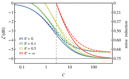
(b)

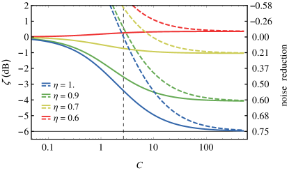
Figure 6: (Color online) Mechanical squeezing $\zeta$ against cooperativity $C$: (a) Varying mechanical bath occupation $\bar{n}=0,\ 1/10,\ 1/2,\ \infty$ (represented by different colors/gray levels) and unit detection efficiency $\eta=1$; The solid (dashed) lines represent a sideband resolution of $\kappa/\omega_{m}=1/10\ (1)$. (b) Different detection efficienies $\eta=1,\,9/10,\,7/10,\,6/10$ (represented by different colors/gray levels) and $\kappa=\omega_{m}/10$; Here the solid (dashed) lines represent $\bar{n}=0\ (\infty)$. In both plots the horizontal solid line at $\zeta=-6\mathrm{dB}$ (corresponding to $N\approx 0.56$) shows the squeezing level of the input light and the vertical dashed line the critical cooperativity $C_{\mathrm{crit}}\approx 2.7$.

Figure 6 shows the steady-state squeezing $\zeta$ transmitted to the mechanical mode for different parameters plotted against the optomechanical cooperativity $C=4g^{2}/(\bar{n}+1)\gamma\kappa$. In the upper plot we assume perfect detection efficiency $\eta=1$ and find that in this case there exists a critical value $C_{\mathrm{crit}}(N)=1/[\sqrt{N(N+1)}]$ determined by the input squeezing $N$ above which the resulting mechanical state is squeezed for any thermal occupation number $\bar{n}$. The lower plot clearly shows that this is no longer true if we assume non-unit detection efficiency $\eta$. We find that below a certain critical value $\eta_{\mathrm{crit}}(N,\bar{n})$ we can no longer transfer squeezing to the mechanical oscillator, but we rather heat it instead. (This is even true for a zero-temperature mechanical environment, as illustrated in the plot.) In this general case it can be beneficial to chose a modified feedback gain, i. e., use feedback operators $\tilde{F}_{\pm}=\sigma F_{\pm}$ with $\sigma\neq 1$. In the parameter regime we consider however the resulting improvement negligible.

II.5 Time-continuous optomechanical entanglement swapping

We now replace the squeezed field mode with a second optomechanical cavity, as is depicted in Fig. 1(c). The goal of this scheme is to generate stationary entanglement between the two mechanical subsystems. This is again facilitated by a time-continuous Bell measurement—measuring the output light of both cavities—plus feedback Hofer et al. (2013). The implementation is akin to the teleportation protocol presented above: Both cavities are driven on the blue sideband to resonantly enhance the two-mode squeezing interaction, and their output light is sent to the Bell detection setup which operates at the cavity resonance frequency $\omega_{c}$. Feeding back the Bell detection results $I_{\pm}$ corresponding to the $x_{+}$ and $p_{-}$ quadratures of the optical fields to both mechanical systems dissipatively drives them towards an entangled state. There is a slight complication, however. A single Bell measurement only allows us to separately monitor two of the four variables ($x_{m,1},p_{m,1},x_{m,2},p_{m,2}$) needed to describe the quantum state of the mechanical systems. Combined with the fact that we drive the system on the blue side of the cavity resonance (and thus in an unstable regime) this means that we cannot actively stabilize the system and—depending on the driving strength and sideband resolution—no steady state may exist. To compensate for this we extend the setup by two additional heterodyne detectors, measuring $x_{-}$ and $p_{+}$ with outcomes $I^{\prime}_{\mp}$. The effective measurement strength of this stabilizing measurements with respect to the Bell measurement is set by the transmissivity $\upsilon$ of the beam-splitter in front of the heterodyne setup (see Fig. 1). Appropriate feedback of all measurement currents $I_{\pm}$, $I^{\prime}_{\pm}$ (for simplicity labeled $I_{i}$, $i=1,\dots,4$, below) to both mechanical systems finally allows us to stabilize them in an entangled state. Note that this setup effectively realizes two simultaneous Bell measurements of the pairs ($x_{+},p_{-}$) and ($x_{-},p_{+}$) with detection efficiencies $\upsilon$ and $1-\upsilon$ respectively. In the rest of this section the two optomechanical systems are assumed to be identical and all detectors to have the same quantum detection efficiency $\eta$.

In Sec. III.4.2 we show that in an adiabatic approximation the conditional state of the two mechanical oscillators $\rho^{(m)}$ in a rotating frame can be described by the SME (setting $\Delta_{l}=\omega_{m}$)

$$\operatorname{d}\!\rho^{(m)}_{c}=\epsilon\frac{4g^{2}}{\kappa}\left(\mathcal{D}[c_{m,1}]\rho^{(m)}_{c}+\mathcal{D}[c_{m,2}]\rho^{(m)}_{c}\right)\operatorname{d}\!t\\ +\sum_{i=1}^{2}\left\{\gamma(\bar{n}+1)\mathcal{D}[c_{m,i}]\rho^{(m)}_{c}+\gamma\bar{n}\mathcal{D}[c_{m,i}^{\dagger}]\rho^{(m)}_{c}\right\}\operatorname{d}\!t\\ +\frac{2g^{2}}{\kappa}\sum_{i=1}^{4}\left(\mathcal{D}[J_{i}]\rho^{(m)}_{c}\operatorname{d}\!t+\sqrt{\eta}\mathcal{H}[J_{i}]\rho^{(m)}_{c}\operatorname{d}\!W_{i}\right),$$ (16)

where we set $(J_{1},J_{2})=\sqrt{\upsilon}\bigl{(}c_{m,+},\mathrm{i}c_{m,-}\bigr{)}$, $(J_{3},J_{4})=\sqrt{1-\upsilon}(\mathrm{i}c_{m,+},c_{m,-})$ and $c_{m,\pm}=c_{m,1}\pm c_{m,2}$. The Wiener processes $W_{i}$ are uncorrelated with unit variance, i. e., $\operatorname{d}\!W_{i}\operatorname{d}\!W_{j}=\delta_{ij}\operatorname{d}\!t$, and correspond to the photo-currents

$$I_{i}\operatorname{d}\!t=\sqrt{4g^{2}/\kappa}\langle J_{i}+J_{i}^{\dagger}\rangle_{c}\operatorname{d}\!t+\operatorname{d}\!W_{i}.$$ (17)

The final steady state of this protocol depends on the feedback operators $F_{i}=F_{i}^{\dagger}$ we apply. In ananolgy to the previous section we choose $(F_{1},F_{2})=\sqrt{\upsilon}\sigma(\mathrm{i}c_{+}-\mathrm{i}c_{+}^{\dagger},c_{-}+c_{-}^{\dagger})$ and $(F_{3},F_{4})=\sqrt{1-\upsilon}(c_{+}+c_{+}^{\dagger},\mathrm{i}c_{-}-\mathrm{i}c_{-}^{\dagger})$, which can realize independent displacements of all mechanical quadratures. This time we introduced an additional gain parameter $\sigma$ which we can vary in order to optimize the amount of entanglement in the resulting steady state. With these choices the FME for optomechanical entanglement swapping takes the form

$$\dot{\rho}^{(m)}_{c}=-\mathrm{i}[H_{\mathrm{fb}},\rho^{(m)}_{c}]+\epsilon\frac{4g^{2}}{\kappa}\left(\mathcal{D}[c_{m,1}]+\mathcal{D}[c_{m,2}]\right)\rho^{(m)}_{c}\\ +\sum_{i=1}^{2}\left\{\gamma(\bar{n}+1)\mathcal{D}[c_{m,i}]\rho^{(m)}_{c}+\gamma\bar{n}\mathcal{D}[c_{m,i}^{\dagger}]\rho^{(m)}_{c}\right\}\\ +\frac{2g^{2}}{\kappa}\sum_{i=1}^{4}\left\{\mathcal{D}[J_{i}-\mathrm{i}F_{i}]\rho^{(m)}_{c}+\frac{1-\eta}{\eta}\mathcal{D}[F_{i}]\right\},$$ (18)

where the dynamics generated by the feedback is described by $H_{\mathrm{fb}}=\mathrm{i}[(1+\sigma)\upsilon-1](2g^{2}/\kappa)(c_{m,+}^{2}+c_{m,-}^{2}-\mathrm{H.\,c.}{})$. We can now analyze the stability properties of the linear feedback system by evaluating the corresponding Routh–Hurwitz criterion. In the case of no stabilizing feedback ($\upsilon=1$) we find that the admissible optomechanical coupling is limited from above by $4g^{2}/\kappa<1/(1-\epsilon)$, which only gives an appreciably high limit for values of $\epsilon\approx 1$ and thus in the bad-cavity regime. The stabilization is caused by the counter-rotating beam-splitter terms $c_{m,i}c_{l,i}^{\dagger}+\mathrm{H.\,c.}{}$ of the optomechanical Hamiltonian, which cool the mechanical systems. This cooling effect, however, diminishes the amount of generated steady-state entanglement. If we switch on the stabilizing feedback and thus choose $\upsilon<1$, we can rewrite the RH criterion in the form $[3+(4g^{2}/\kappa)^{-1}+\epsilon]>4\upsilon>[(1-\epsilon)-(4g^{2}/\kappa)^{-1}]/\sigma$ (where we assumed $\epsilon<1$). These inequalities are tightest in the limit $\epsilon\rightarrow 0$, $g^{2}/\kappa\rightarrow\infty$ where we have $3>4\upsilon>1/\sigma$. For the rest of this section we choose $\upsilon=3/4$ which ensures stability of the feedback system for any values of $g^{2}/\kappa$ and $\epsilon$—and consequently the sideband-resolution $\kappa/\omega_{m}$—as long as the feedback gain fulfills $\sigma>1/3$. In the stable regime and for $\epsilon=0$, $\eta=1$ we find a simple analytic expression for the steady-state logarithmic negativity,

$$E^{\mathrm{ss}}_{\mathcal{N}}=\ln\left(\frac{\frac{1}{2}C(\bar{n}+1)(3\sigma-1)(4\upsilon-1)+1}{C(\bar{n}+1)[3\sigma(\sigma-1)+1]+2\bar{n}+1}\right),$$ (19)

where we again introduced the cooperativity $C=4g^{2}/(\bar{n}+1)\gamma\kappa$. Generally we can—for each set of parameters $(C,\bar{n},\epsilon,\upsilon,\eta)$—maximize the entanglement $E_{\mathcal{N}}$ with respect to the feedback gain $\sigma$. In Fig. 7 we plot the resulting steady-state values in terms of logarithmic negativity $E_{\mathcal{N}}$ and EPR-variance

$$\Delta_{\mathrm{EPR}}=\min_{\phi_{1},\phi_{2}}\left([\Delta(x_{m,1}^{\phi_{1}}-x_{m,2}^{\phi_{2}})]^{2}+[\Delta(p_{m,1}^{\phi_{1}}+p_{m,2}^{\phi_{2}})]^{2}\right),$$ (20)

where $x_{m,i}^{\phi}=(c_{m,i}\mathrm{e}^{-\mathrm{i}\phi}+c_{m,i}^{\dagger}\mathrm{e}^{+\mathrm{i}\phi})/\sqrt{2}$ and $p_{m,i}^{\phi}=x_{m,i}^{\phi+\pi/2}$ are rotated mechanical quadratures. A Gaussian state is entangled if $\Delta_{\mathrm{EPR}}<2$ Duan et al. (2000); Simon (2000). In the first plot we assume a perfect detection efficiency $\eta=1$ and consider different bath occupation numbers $\bar{n}$. We again see that there exists a critical cooperativity $C_{\mathrm{crit}}$ above which we are able to generate entanglement regardless of $\bar{n}$. From (19) we can deduce the expression $C_{\mathrm{crit}}(\upsilon,\sigma)=4/[3\sigma(1+4\upsilon-2\sigma)-(1+4\upsilon)]$. (As is evident from the plot, the $C_{\mathrm{crit}}$ is independent of $\epsilon$). For the parameters used in the plot (taking into account the optimization with respect to $\sigma$) we find $C_{\mathrm{crit}}=2$. Again, counter-rotating terms decrease entanglement but are strongly suppressed by the sideband resolution. In Fig. 7(b) we take into account losses and non-unit detection efficiency, $\eta<1$, which drastically reduces the amount of achieved entanglement. As before we find a critical loss value $\eta_{\mathrm{crit}}(\bar{n},\upsilon)$ (for the parameters chosen in the plot slightly above 65%) below which entanglement creation is prohibited.

(a)

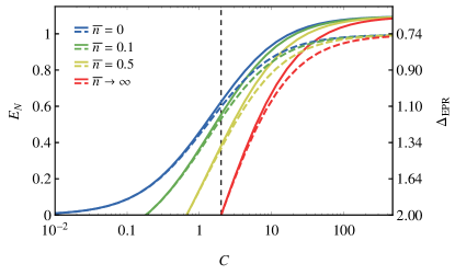
(b)

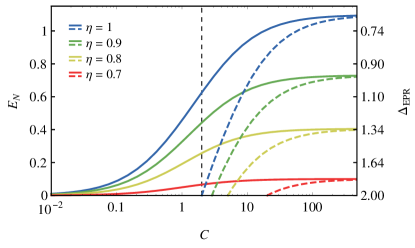
Figure 7: (Color online) Two-mode mechanical steady-state entanglement in terms of $E^{\mathrm{ss}}_{\mathcal{N}}$ and $\Delta_{\mathrm{EPR}}$ against cooperativity $C$, maximized with respect to feedback gain $\sigma$: (a) Varying mechanical bath occupation $\bar{n}=0,\,1/10,\,1/2,\,\infty$ (represented by different colors/gray levels) for unit detection efficiency $\eta=1$; The solid (dashed) lines represent a sideband resolution of $\kappa/\omega_{m}=1\ (1/10)$. (b) Different detection efficienies $\eta=1,\,9/10,\,7/10,\,6/10$ (represented by different colors/gray levels) and $\kappa=\omega_{m}/10$; Here the solid (dashed) lines represent $\bar{n}=0\ (\infty)$. The black vertical line shows the critical cooperativity $C_{\mathrm{crit}}=2$.

III Derivation of conditional and feedback master equations

We present here a brief (and informal) derivation of the stochastic master equations (SME) and Markovian feedback master equations (FME) we use throughout the paper. A rigorous and complete account of the quantum stochastic formalism and quantum filtering theory can be found in the literature, e. g., Hudson and Parthasarathy (1984); Carmichael (1993a); Zoller and Gardiner (1997); Bouten et al. (2007); Barchielli and Gregoratti (2009); Wiseman and Milburn (2009), and a brief summary of the most important relations is given in App. A.

III.1 The homodyne master equation

We consider a situation similar to Fig. 1(a), where a system $S$ couples to the one-dimensional electromagnetic field $A$, which is initially in vacuum and is subject to homodyne detection. We first assume unit detection efficiency, but will discuss the case of inefficient detection at the end of the section. The system–field coupling is mediated by the Hamiltonian

$$H_{\mathrm{int}}=\mathrm{i}[s\,a^{\dagger}(t)-s^{\dagger}a(t)],$$ (21)

where $s$ is a system operator (e. g., a cavity creation or destruction operator), and the light field is described (in an interaction picture at a central frequency $\omega_{0}$) by $a(t)=\int\operatorname{d}\!\omega\,a_{0}(\omega)\,\mathrm{e}^{-\mathrm{i}(\omega-\omega_{0})t}$ Gardiner and Collett (1985), where $a_{0}(\omega)$ is the (Schrödinger) annihilation operator of the field mode at $\omega$. In a Markov approximation the field operators are $\delta$-correlated, and fulfill the commutation relations

$$[a(t),a^{\dagger}(t^{\prime})]=\delta(t-t^{\prime}).$$ (22)

Under this approximation we can introduce the Itō increments $\operatorname{d}\!A$, $\operatorname{d}\!A^{\dagger}$, which (formally) obey $\operatorname{d}\!A(t)=a(t)\operatorname{d}\!t$, etc., and the vacuum multiplication table given in App. A.

The Schrödinger equation for the full system ($S+A$) initially in the state $|\phi_{0}\rangle=|\psi_{0}\rangle_{S}|\mathrm{vac}\rangle_{A}$ can be written in Itō-form as

$$\operatorname{d}\!|\phi(t)\rangle=\left\{-\mathrm{i}H_{\mathrm{eff}}\operatorname{d}\!t+s\left[\operatorname{d}\!A^{\dagger}(t)+\operatorname{d}\!A(t)\right]\right\}|\phi(t)\rangle,$$ (23)

where we used the fact that $\operatorname{d}\!A(t)|\phi(t)\rangle=\operatorname{d}\!A(t)|\phi_{0}\rangle=\operatorname{d}\!A(t)|\mathrm{vac}\rangle=0$ Gardiner and Zoller (2004). A homodyne measurement of an electromagnetic quadrature $x=a+a^{\dagger}$ with a result $I_{x}$ effectively projects the state of the light field onto the eigenstate $|I_{x}\rangle$ of $x$, where $x|I_{x}\rangle=I_{x}|I_{x}\rangle$ Goetsch and Graham (1994). Projecting (23) onto $|I_{x}\rangle$ leads to the linear stochastic Schrödinger equation (SSE) Carmichael (1993b)

$$\operatorname{d}\!|\tilde{\psi}_{c}(t)\rangle=\left[-\mathrm{i}H_{\mathrm{eff}}\operatorname{d}\!t+\,s\,I_{x}(t)\operatorname{d}\!t\right]|\psi_{c}(t)\rangle,$$ (24)

with the forward pointing Itō-increment $\operatorname{d}\!|\tilde{\psi}_{\mathrm{c}}(t)\rangle={|\tilde{\psi_{c}}(t+\operatorname{d}\!t)\rangle}-|\psi_{c}(t)\rangle$. $|\tilde{\psi}_{c}\rangle$ is the unnormalized system state which is conditioned on the homodyne photo-current $I_{x}$. $I_{x}$ is $\delta$-correlated, i. e., $\langle I_{x}(t)I_{x}(s)\rangle=\delta(t-s)$, and its probability distribution is given (for a fixed time $t$) by $\Upsilon_{t}(I_{x})=|\langle I_{x}|\phi(t+\operatorname{d}\!t)\rangle|^{2}$ Goetsch and Graham (1994); Wiseman and Milburn (2009). Using this, one can show that $I_{x}$ can be written as Gardiner and Zoller (2004); Wiseman and Milburn (2009)

$$I_{x}(t)\operatorname{d}\!t=\langle s+s^{\dagger}\rangle_{c}(t)\operatorname{d}\!t+\operatorname{d}\!W(t),$$ (25)

where $W$ is a classical Wiener process with $\operatorname{d}\!W(t)^{2}=\operatorname{d}\!t$ and $\mathbb{E}[\operatorname{d}\!W(t)]=0$. Here the conditional expectation value should be read as $\langle A\rangle_{c}(t)=\langle\psi_{c}(t)|A|\psi_{c}(t)\rangle$. We can introduce the classical stochastic process $\widetilde{X}$ defined by $\operatorname{d}\!\widetilde{X}(t)=I_{x}(t)\operatorname{d}\!t$, which is statistically equivalent to $\operatorname{d}\!A(t)+\operatorname{d}\!A(t)^{\dagger}$. This is due to non-demolition properties of the measurement operator, see Bouten et al. (2007). It obeys $\operatorname{d}\!\widetilde{X}(t)^{2}=\operatorname{d}\!t$.

The corresponding equation of motion for the unnormalized conditional state $\tilde{\rho}_{c}=|\tilde{\psi_{c}}\rangle\langle\tilde{\psi_{c}}|$ can be deduced from (24),

$$\operatorname{d}\!\tilde{\rho}_{c}(t) =\tilde{\rho}_{c}(t+\operatorname{d}\!t)-\rho_{c}(t)$$

$$=\mathcal{L}\rho_{c}(t)\operatorname{d}\!t+\left[s\rho_{c}(t)+\rho_{c}(t)s^{\dagger}\right]\operatorname{d}\!\widetilde{X}(t)$$ (26)

where we used Itō calculus as presented in App. A. Here the Liouvillian $\mathcal{L}$ is given by

$$\mathcal{L}{\rho}=-\mathrm{i}\left(H_{\mathrm{eff}}{\rho}-{\rho}H_{\mathrm{eff}}^{\dagger}\right)+s{\rho}s^{\dagger}.$$ (27)

Equation (26) is the quantum analog to the classical Zakai equation Xiong (2008). Note that although the Liouvillian is trace-preserving (i. e., $\mathrm{tr}[\mathcal{L}\rho]=0$), the second term in (26) does not possess this property. The equation for the normalized state $\rho_{c}(t)=\tilde{\rho}_{c}(t)/\mathrm{tr}[\tilde{\rho}_{c}(t)]$ is then found by noting that

$$\mathrm{tr}[\tilde{\rho}_{c}(t+\operatorname{d}\!t)]=1+\langle s+s^{\dagger}\rangle_{c}(t)\operatorname{d}\!\widetilde{X}(t),$$ (28)

where now $\langle A\rangle_{c}=\mathrm{tr}[\rho_{c}(t)A]$ and we used $\mathrm{tr}[\rho_{c}(t)]=1$. Thus we find

$$\mathrm{tr}[\tilde{\rho}_{c}(t+\operatorname{d}\!t)]^{-1}=1-\langle s+s^{\dagger}\rangle_{c}(t)\operatorname{d}\!\widetilde{X}(t)+[\langle s+s^{\dagger}\rangle_{c}(t)]^{2}\operatorname{d}\!t,$$ (29)

which is obtained by expanding $\mathrm{tr}[\tilde{\rho}_{c}(t+\operatorname{d}\!t)]^{-1}$ to second order in $\operatorname{d}\!\widetilde{X}$ (which leads to a first-order expansion in $\operatorname{d}\!t$). Using Itō multiplication rules this leads to

$$\operatorname{d}\!\rho_{c}(t) =\frac{\tilde{\rho}_{c}(t+\operatorname{d}\!t)}{\mathrm{tr}[\tilde{\rho}_{c}(t+\operatorname{d}\!t)]}-\rho_{c}(t)$$

$$=\mathcal{L}\rho_{c}(t)\operatorname{d}\!t+\mathcal{H}[s]\rho_{c}(t)\operatorname{d}\!W(t),$$ (30)

which is the desired result Gardiner and Zoller (2004); Wiseman and Milburn (2009). The (nonlinear) measurement term is given by

$$\mathcal{H}[s]\rho_{c}=\bigl{(}s-\mathrm{tr}[\rho_{c}s]\bigr{)}\rho_{c}+\rho_{c}\bigl{(}s-\mathrm{tr}[\rho_{c}s]\bigr{)}^{\dagger}.$$ (31)

It is clear from the derivation that under made assumptions the SSE (24) is equivalent to the SME (30). The stochastic master equation is more general, however, as it can accommodate for additional, unobserved decay channels (such as photon losses/inefficient detection or coupling of a mechanical oscillator to a heat bath), as well as for mixed initial states.

We can generalize the homodyne master equation in several ways: Above we assumed a measurement of a specific light quadrature $x=a+a^{\dagger}$. To measure a rotated quadrature $x^{\phi}=a\mathrm{e}^{-\mathrm{i}\phi}+a^{\dagger}\mathrm{e}^{+\mathrm{i}\phi}$ we have to make the replacement $s\rightarrow\mathrm{e}^{\mathrm{i}\phi}s$, which simply follows from replacing $a\rightarrow\mathrm{e}^{-\mathrm{i}\phi}a$. We can as easily obtain the SME corresponding to heterodyne detection at a LO frequency $\omega_{\mathrm{lo}}\neq\omega_{0}$ by substituting $s\rightarrow\mathrm{e}^{\mathrm{i}\Delta_{\mathrm{lo}}t}s$, where $\Delta_{\mathrm{lo}}=\omega_{\mathrm{lo}}-\omega_{0}$. Below we will discuss the situation where we split up the field with a beam-splitter (with a splitting ration $\eta:1-\eta$) and perform two simultaneous homodyne measurements on its outputs. The measured modes $A^{\prime}$, $B$ after the beam-splitter [see Fig. 1(a)] are related to $A$ before the beam-splitter via Gough and James (2009) $a(t)=\sqrt{\eta}\,a^{\prime}(t)+\sqrt{1-\eta}\,b(t)$, where $A^{\prime}$ and $B$ are both initially in vacuum and are uncorrelated such that $\operatorname{d}\!A(t)\operatorname{d}\!B^{\dagger}(t)=0$, etc. Plugging this relation into (23) and projecting onto the quadratures $\mathrm{e}^{-\mathrm{i}\phi_{1}}a^{\prime}+\mathrm{e}^{\mathrm{i}\phi_{1}}a^{\prime\dagger}$, $\mathrm{e}^{-\mathrm{i}\phi_{2}}b+\mathrm{e}^{\mathrm{i}\phi_{2}}b^{\dagger}$ one can repeat above steps and find

$$\operatorname{d}\!\rho_{c}=\mathcal{L}\rho_{c}\operatorname{d}\!t+\sqrt{\eta}\mathcal{H}[\mathrm{e}^{\mathrm{i}\phi_{1}}s]\rho_{c}\operatorname{d}\!W_{1}\\ +\sqrt{1-\eta}\mathcal{H}[\mathrm{e}^{\mathrm{i}\phi_{2}}s]\rho_{c}\operatorname{d}\!W_{2},$$ (32)

with uncorrelated Wiener processes $W_{i}$, i. e., $\operatorname{d}\!W_{i}\operatorname{d}\!W_{j}=\delta_{ij}$. To model photon losses or inefficient photo-detectors, we average over, say, the second measurement process, and thus discard all information obtained from it. Due to the fact that $\operatorname{\mathbb{E}}[\operatorname{d}\!W_{2}]=0$, the equation of motion for the resulting conditional state—which is now conditioned on the measurement results of the first channel only—is obtained by dropping the last term in (32). The beam-splitter transmissivity is then identified with the efficiency of the photo-detection. Formally we can obtain the same result from (30) by replacing $s\rightarrow\sqrt{\eta}s$ in the measurement term, while keeping the Liouvillian unchanged.

III.2 Time-continuous teleportation

III.2.1 Conditional master equation

We now extend the derivation of the homodyne SME presented in the previous section to the Bell-measurement setup depicted in Fig. 1(b). Again, a one-dimensional field mode $A$ [described by $a(t)$] couples to a system $S$ via (21). $A$ is assumed to be in the vacuum state. A second field mode, $B$ [with a field operator $b(t)$] is prepared in a pure squeezed state, parametrized by $M\in\mathbb{C}$, which we simply denote by $|M\rangle$. $M$ describes the degree and angle of squeezing, as described in App. C. The Itō multiplication table for $B$ is thus given by

$\times$	$\operatorname{d}\!B$	$\operatorname{d}\!B^{\dagger}$	$\operatorname{d}\!t$
$\operatorname{d}\!B$	$M\operatorname{d}\!t$	$(N+1)\operatorname{d}\!t$	0
$\operatorname{d}\!B^{\dagger}$	$N\operatorname{d}\!t$	$M^{*}\operatorname{d}\!t$	0
$\operatorname{d}\!t$	0	0	0

with the condition $|M|^{2}=N(N+1)$. $A$ and $B$ are combined on a balanced beam splitter, whose output is sent to two homodyne detection setups, which are set up such that they measure the EPR operators $x_{+}=(a+a^{\dagger}+b+b^{\dagger})/\sqrt{2}$ and $p_{-}=\mathrm{i}(a-a^{\dagger}-b+b^{\dagger})/\sqrt{2}$. We call the continuous measurement of the two quadratures $x_{+}$ and $p_{-}$ a time-continuous Bell measurement Hofer et al. (2013). To find the corresponding SME, describing the state of $S$ conditioned on measurements of $x_{+}$ and $p_{-}$, we apply the same reasoning as in the previous section. We start from the Schrödinger equation (23) but now choose the initial condition $|\phi_{0}\rangle=|\psi_{0}\rangle_{S}|\mathrm{vac}\rangle_{A}|M\rangle_{B}$. Using the eigenvalue equation for squeezed states (89), written as $[\operatorname{d}\!B(t)-\alpha\operatorname{d}\!B(t)]|M\rangle=0$ with $\alpha=(N+M)/(N+M^{*}+1)$, and again $\operatorname{d}\!A(t)|\mathrm{vac}\rangle=0$, we can write

$$\operatorname{d}\!|\phi\rangle =\left\{-\mathrm{i}H_{\mathrm{eff}}\operatorname{d}\!t+s\left[\operatorname{d}\!A^{\dagger}-\alpha\operatorname{d}\!A+\operatorname{d}\!B-\alpha\operatorname{d}\!B^{\dagger}\right]\right\}|\phi\rangle$$

$$=\left\{-\mathrm{i}H_{\mathrm{eff}}\operatorname{d}\!t+\sqrt{1/2}\,s\left[\mu\operatorname{d}\!X_{+}+\mathrm{i}\nu\operatorname{d}\!P_{-}\right]\right\}|\phi\rangle,$$ (33)

where $\mu=1-\alpha$, $\nu=1+\alpha$ and $\operatorname{d}\!X_{+}(t)=x_{+}(t)\operatorname{d}\!t$, $\operatorname{d}\!P_{-}(t)=p_{-}(t)\operatorname{d}\!t$. Going from the first to the second line we used the fact that $a^{\dagger}+b=(x_{+}+\mathrm{i}p_{-})/\sqrt{2}$. We emphasize that $x_{+}$ and $p_{-}$ commute and can be measured simultaneously. We can thus directly project equation (III.2.1) onto the EPR state $|I_{+}I_{-}\rangle_{AB}$ defined by $x_{+}|I_{+}I_{-}\rangle_{AB}=I_{+}|I_{+}I_{-}\rangle_{AB}$ and $p_{-}|I_{+}I_{-}\rangle_{AB}=I_{-}|I_{+}I_{-}\rangle_{AB}$. This yields the linear stochastic Schrödinger equation

$$\operatorname{d}\!|\tilde{\psi_{c}}\rangle=\left\{-\mathrm{i}H_{\mathrm{eff}}\operatorname{d}\!t+\sqrt{1/2}\,s[\mu\operatorname{d}\!\widetilde{X}_{+}+\mathrm{i}\nu\operatorname{d}\!\widetilde{P}_{-}]\right\}|\psi_{c}\rangle,$$ (34)

where $\operatorname{d}\!\widetilde{X}_{+}(t)=I_{+}(t)\operatorname{d}\!t$ and $\operatorname{d}\!\widetilde{P}_{-}(t)=I_{-}(t)\operatorname{d}\!t$ are again classical processes which possess the same statistical properties as their quantum counterparts. The photo-currents $I_{\pm}$ (analogous to the previous section) can be written as

$$I_{+}\operatorname{d}\!t =\sqrt{1/2}\langle s+s^{\dagger}\rangle_{c}\operatorname{d}\!t+\operatorname{d}\!W_{+},$$ (35a)

$$I_{-}\operatorname{d}\!t =\mathrm{i}\sqrt{1/2}\langle s-s^{\dagger}\rangle_{c}\operatorname{d}\!t+\operatorname{d}\!W_{-},$$ (35b)

with Wiener increments $\operatorname{d}\!W_{\pm}$. Comparison to the output of a single homodyne setup (25) shows that $I_{\pm}$ correspond to two simultaneous homodyne measurements with half efficiency. The (co-)variances of $\operatorname{d}\!W_{\pm}$ are given in equations (14) and directly follow from the definition of $\operatorname{d}\!X_{+}$, $\operatorname{d}\!P_{-}$ and the multiplication tables for $\operatorname{d}\!A$ and $\operatorname{d}\!B$. We now repeat the procedure from the previous section which is now more involved due to fact that we have to deal with two correlated random processes. It is convenient to introduce the complex process $\operatorname{d}\!Y(t)=\mu\operatorname{d}\!\widetilde{X}_{+}(t)+\mathrm{i}\nu\operatorname{d}\!\widetilde{P}_{-}(t)$, which obeys $\operatorname{d}\!Y^{2}=2\zeta\operatorname{d}\!t{:=}-2N/M^{*}\operatorname{d}\!t$ and $|\operatorname{d}\!Y|^{2}=2\operatorname{d}\!t$. We can then write the Zakai equation corresponding to (34) as

$$\operatorname{d}\!\tilde{\rho_{c}}=\mathcal{L}\rho_{c}\operatorname{d}\!t+\sqrt{1/2}\left(s\rho_{c}\operatorname{d}\!Y+\rho_{c}s^{\dagger}\operatorname{d}\!Y^{*}\right),$$ (36)

with $\mathcal{L}$ defined in (27). To normalize this equation we first calculate

$$\mathrm{tr}[\tilde{\rho_{c}}(t+\operatorname{d}\!t)]=1+\sqrt{1/2}\bigl{[}\langle s\rangle_{c}(t)\operatorname{d}\!Y(t)+\mathrm{H.\,c.}{}\bigr{]},$$ (37)

which we use to obtain (by expanding to second order in $\operatorname{d}\!Y$)

$$\mathrm{tr}[\tilde{\rho_{c}}(t+\operatorname{d}\!t)]^{-1}=1-\sqrt{1/2}\bigl{[}\langle s\rangle_{c}(t)\operatorname{d}\!Y(t)+\mathrm{H.\,c.}{}\bigr{]}\\ +(1/2)\left\{[\langle s\rangle_{c}(t)]^{2}\zeta+[\langle s^{\dagger}\rangle_{c}(t)]^{2}\zeta^{*}+4|\langle s\rangle_{c}(t)|^{2}\right\}\operatorname{d}\!t.$$ (38)

Combining this with (36) we find after some algebra

$$\operatorname{d}\!\rho_{c} =\mathcal{L}\rho_{c}\operatorname{d}\!t+\sqrt{1/2}\left[\mu\bigl{(}s-\langle s\rangle_{c}\bigr{)}\rho_{c}+\mathrm{H.\,c.}{}\right]\rho_{c}\operatorname{d}\!W_{+}$$ (39)

$$\quad+\sqrt{1/2}\left[\mathrm{i}\nu\bigl{(}s-\langle s\rangle_{c}\bigr{)}\rho_{c}+\mathrm{H.\,c.}{}\right]\rho_{c}\operatorname{d}\!W_{-}$$

$$=\mathcal{L}\rho_{c}\operatorname{d}\!t+\sqrt{1/2}\left\{\mathcal{H}[\mu s]\rho_{c}\operatorname{d}\!W_{+}+\mathcal{H}[\mathrm{i}\nu s]\rho_{c}\operatorname{d}\!W_{-}\right\}.$$

It can easily be checked that this is a equation of the form (70) and thus a valid Belavkin equation Belavkin (1992).

To conclude this section let us briefly discuss, as a slight variation of above setup, the situation where instead of the squeezed state $|M\rangle_{B}$ we use a displaced squeezed state $|M,\beta\rangle_{B}=D(\beta)|M\rangle_{B}$ (see App. C) as an initial state of mode $B$, and thus as an input state for teleportation. Transforming the Schrödinger equation (23) into a displaced frame with $D(\beta)$ shows that the structure of the SSE (24) and the SME (39) remains unchanged, if the measurement processes are replaced by appropriately displaced versions, $\operatorname{d}\!\widetilde{X}_{+}\rightarrow\operatorname{d}\!\widetilde{X}_{+}-\sqrt{1/2}(\beta+\beta^{*})\operatorname{d}\!t$ and $\operatorname{d}\!\widetilde{P}_{-}\rightarrow\operatorname{d}\!\widetilde{P}_{-}+\mathrm{i}\sqrt{1/2}(\beta-\beta^{*})\operatorname{d}\!t$. Consequently, the same transformation has to be applied to the currents $I_{\pm}$ in equations (35). A more rigorous derivation of the results in this section is presented in Dabrowska and Gough (2014).

III.2.2 Feedback master equation

We follow Wiseman and Milburn (1993) to apply Markovian (i. e., instantaneous) feedback proportional to the homodyne currents $I_{\pm}$ to the system $S$. This procedure consists of three steps: Converting the Itō-equation for the conditional state into Stratonovich form Gardiner and Zoller (2004), adding a feedback term, and converting back to Itō-form in order to average over all possible measurement trajectories and to obtain an unconditional master equation. The feedback we model as generalized forces $F_{\pm}=F_{\pm}^{\dagger}$ in the form of additional Hamiltonian terms which we write as $\mathcal{K}_{\pm}\rho I_{\pm}=-\mathrm{i}[F_{\pm}I_{\pm},\rho]$.

We start by rewriting the SME (39) in terms of the complex Wiener increment $\operatorname{d}\!W_{y}=\mu\operatorname{d}\!W_{+}+\mathrm{i}\nu\operatorname{d}\!W_{-}$ (this time including the detector efficiency $\eta$ as discussed in Sec. III.1),

$$\operatorname{d}\!\rho_{c}=\mathcal{L}\rho_{c}\operatorname{d}\!t+\sqrt{\eta/2}\left(\mathcal{G}\rho_{c}\operatorname{d}\!W_{y}+\mathcal{G}^{\dagger}\rho_{c}\operatorname{d}\!W_{y}^{*}\right),$$ (40)

where we defined $\mathcal{G}\rho=(s-\mathrm{tr}[s\rho])\rho$ and $\mathcal{G}^{\dagger}\rho=(\mathcal{G}\rho)^{\dagger}$. The Stratonovich form of this equation is given by

$$\begin{split}(\mathbf{S})\quad\operatorname{d}\!\rho_{c}&=\mathcal{L}\rho_{c}\operatorname{d}\!t+\sqrt{\frac{\eta}{2}}\left(\mathcal{G}\rho_{c}\operatorname{d}\!W_{y}+\mathcal{G}^{\dagger}\rho_{c}\operatorname{d}\!W_{y}^{*}\right)\\ &\qquad-\frac{\eta}{4}\left(\mathcal{G}\rho_{c}\operatorname{d}\!W_{y}+\mathcal{G}^{\dagger}\rho_{c}\operatorname{d}\!W_{y}^{*}\right)^{2}\\ &=\mathcal{\bar{L}}\rho_{c}\operatorname{d}\!t+\sqrt{\frac{\eta}{2}}\left(\mathcal{G}\rho_{c}\operatorname{d}\!W_{y}+\mathcal{G}^{\dagger}\rho_{c}\operatorname{d}\!W_{y}^{*}\right),\end{split}$$ (41)

with the definition $\mathcal{\bar{L}}=\mathcal{L}-\tfrac{\eta}{2}[\zeta\mathcal{G}^{2}+\zeta^{*}(\mathcal{G}^{\dagger})^{2}+2\mathcal{G^{\dagger}G}]$. Here we used the fact that $\mathcal{G^{\dagger}G}=\mathcal{GG^{\dagger}}$. Adding feedback terms $[\dot{\rho}_{c}]_{\mathrm{fb}}=\sqrt{1/2\eta}[\mathcal{K}_{+}I_{+}+\mathcal{K}_{-}I_{-}]$ and converting back to Itō form yields

$$\operatorname{d}\!\rho_{c}=\mathcal{L}\rho_{c}+(1/4\eta)\bigl{(}\mathcal{K}_{+}\operatorname{d}\!\widetilde{X}_{+}+\mathcal{K}_{-}\operatorname{d}\!\widetilde{P}_{-}\bigr{)}^{2}\rho_{c}\\ +(1/2)\bigl{(}\mathcal{K}_{+}\operatorname{d}\!\widetilde{X}_{+}+\mathcal{K}_{-}\operatorname{d}\!\widetilde{P}_{-}\bigr{)}\left(\mathcal{G}\operatorname{d}\!W_{y}+\mathcal{G}^{\dagger}\operatorname{d}\!W_{y}^{*}\right)\rho_{c}\\ +\sqrt{1/2\eta}\bigl{(}\mathcal{K}_{+}\operatorname{d}\!\widetilde{X}_{+}+\mathcal{K}_{-}\operatorname{d}\!\widetilde{P}_{-}\bigr{)}\\ +\sqrt{\eta/2}\left(\mathcal{G}\operatorname{d}\!W_{y}+\mathcal{G}^{\dagger}\operatorname{d}\!W_{y}^{*}\right)\rho_{c},$$ (42)

where we chose an ordering $\mathcal{KG}$ to get a trace preserving master equation Wiseman and Milburn (1993). We can now average over all possible measurement trajectories (i. e., over all classical processes $\widetilde{X}_{+}$, $\widetilde{P}_{-}$, $W_{y}$) to obtain an unconditional (deterministic) master equation. A longish calculation leads to

$$\dot{\rho}=\mathcal{L}\rho+\frac{1}{2}\left\{\frac{w_{1}-w_{3}}{\eta}\mathcal{D}[F_{+}]-\mathrm{i}[F_{+},s\rho+\rho s^{\dagger}]\right\}\\ +\frac{1}{2}\left\{\frac{w_{2}-w_{3}}{\eta}\mathcal{D}[F_{-}]-\mathrm{i}[F_{-},(\mathrm{i}s)\rho+\rho(\mathrm{i}s)^{\dagger}]\right\}\\ +\frac{w_{3}}{2\eta}\mathcal{D}[F_{+}+F_{-}],$$ (43)

where we used the fact that $\tfrac{1}{2}(\mathcal{K}_{\pm})^{2}=\mathcal{D}[F_{\pm}]$ and $\tfrac{1}{2}(\mathcal{K_{+}K_{-}}+\mathcal{K_{-}K_{+}})=\mathcal{D}[F_{+}+F_{-}]-\mathcal{D}[F_{-}]-\mathcal{D}[F_{+}]$. $w_{i}$ are the (co-)variances of $\operatorname{d}\!W_{+}$, $\operatorname{d}\!W_{-}$ and are given by (14). Using the identity $\mathcal{D}[s+\mathrm{i}F_{\pm}]\rho=\mathcal{D}[s]\rho+\mathcal{D}[F_{\pm}]\rho+\mathrm{i}[F_{\pm},s\rho+\rho s^{\dagger}]+\tfrac{\mathrm{i}}{2}[\rho,F_{\pm}s+s^{\dagger}F_{\pm}]$ this can be written in the more familiar form

$$\dot{\rho}=-\mathrm{i}\left[H+(1/4)\left\{(F_{+}+\mathrm{i}F_{-})s+s^{\dagger}(F_{+}-\mathrm{i}F_{-})\right\},\rho\right]\\ +(1/2)\big{\{}\mathcal{D}[s-\mathrm{i}F_{+}]\rho+\mathcal{D}[s-F_{-}]\rho+\frac{w_{3}}{\eta}\mathcal{D}[F_{+}+F_{-}]\rho\\ +\left(\frac{w_{1}-w_{3}}{\eta}-1\right)\mathcal{D}[F_{+}]\rho+\left(\frac{w_{2}-w_{3}}{\eta}-1\right)\mathcal{D}[F_{-}]\rho\big{\}}.$$ (44)

If we consider again the situation where we use a displace squeezed state $|M,\beta\rangle_{B}$ as input, we make the replacements $\operatorname{d}\!\widetilde{X}_{+}\rightarrow\operatorname{d}\!\widetilde{X}_{+}-\sqrt{1/2}(\beta+\beta^{*})\operatorname{d}\!t$ and $\operatorname{d}\!\widetilde{P}_{-}\rightarrow\operatorname{d}\!\widetilde{P}_{-}+\mathrm{i}\sqrt{1/2}(\beta-\beta^{*})\operatorname{d}\!t$ in equation (42). This only changes the third line as all products $\operatorname{d}\!\widetilde{X}^{2}$, $\operatorname{d}\!\widetilde{X}\operatorname{d}\!W_{y}$, etc. are unaffected. After taking the classical average this yields an additional Hamiltonian term $H_{\mathrm{coh}}=\sqrt{2}[\operatorname{Re}(\beta)F_{+}-\operatorname{Im}(\beta)F_{-}]$ which has to be incorporated into $\mathcal{L}$ in the FME (43).

Note that equation (44) is not necessarily a Lindblad equation, as the prefactors to the operators $\mathcal{D}$ may in general be negative. It can easily be brought into Lindblad form, however, see App. D.

III.3 Time-continuous entanglement swapping

III.3.1 Conditional master equation

Consider the setup depicted in 1(c): Two systems $S_{1}$ and $S_{2}$ couple to field modes $A$ and $B$ (described by field operators $a$ and $b$, both in vacuum) via interaction Hamiltonians analog to (21). $A$ and $B$ are combined on a 50:50 beam-splitter to form the combinations $a\pm b$ in the outputs. These outputs are sent to a pair of beam-splitters (with an uneven splitting ratio ${\upsilon:1-\upsilon}$) and subsequently to a total of four homodyne setups. If we label the modes incident on the homodyne detectors as $C_{i}$ (described by field operators $c_{i}$) for $i=1\dots 4$ [see Fig. 1(d)], we find the following relations to modes $A$ and $B$,

$$a =\sqrt{\upsilon/2}(c_{1}+c_{2})-\sqrt{(1-\upsilon)/2}(c_{3}+c_{4}),$$ (45)

$$b =\sqrt{\upsilon/2}(c_{1}-c_{2})-\sqrt{(1-\upsilon)/2}(c_{3}-c_{4}).$$ (46)

We now choose the LO phases of the four homodyne setups such that they measure $x_{+}{=}c_{1}+c_{1}^{\dagger}$, $p_{-}{=}-\mathrm{i}(c_{2}-c_{2}^{\dagger})$, $x_{-}{=}c_{4}+c_{4}^{\dagger}$ and $p_{+}{=}-\mathrm{i}(c_{3}-c_{3}^{\dagger})$. These four measurements allow us to simultaneously monitor both quadratures of both systems (although with imperfect precision). The measurement of $x_{+}$ and $p_{-}$, which we choose to have a relative strength $\upsilon$ set by the beam-splitting ratio, realize a Bell measurement as before, while the measurement of the conjugate quadratures $x_{-}$ and $p_{+}$, with a strength $1-\upsilon$, we will need for stabilization of $S_{1}$ and $S_{2}$.

To derive the SME we apply the same logic as before. We start from the Schrödinger equation for the full system ($S_{1}+S_{2}+\text{field modes}$),

$$\operatorname{d}\!|\phi\rangle=\left[-\mathrm{i}H_{\mathrm{eff}}\operatorname{d}\!t+s_{1}\operatorname{d}\!A^{\dagger}+s_{2}\operatorname{d}\!B^{\dagger}\right]|\phi\rangle,$$ (47)

with an initial state $|\phi\rangle=|\psi(0)\rangle_{S_{1}S_{2}}|\mathrm{vac}\rangle_{\mathrm{field}}$ and an effective Hamiltonian $H_{\mathrm{eff}}=H_{\mathrm{sys}}^{\mathrm{(1)}}+H_{\mathrm{sys}}^{\mathrm{(2)}}-\frac{\mathrm{i}}{2}\sum_{i=1,2}s_{i}^{\dagger}s_{i}$. We then rewrite this in terms of $\operatorname{d}\!X_{\pm}$ and $\operatorname{d}\!P_{\pm}$ and project onto eigenstates corresponding to measurement outcomes $I_{\pm}$, $I^{\prime}_{\pm}$. With the definition $s_{\pm}=s_{1}\pm s_{2}$ we find

$$\operatorname{d}\!|\tilde{\psi}_{c}\rangle=-\mathrm{i}H_{\mathrm{eff}}|\psi_{c}\rangle\operatorname{d}\!t\\ +\sqrt{\upsilon/2}[s_{+}\operatorname{d}\!\widetilde{X}_{+}+\mathrm{i}s_{-}\operatorname{d}\!\widetilde{P}_{-}]|\psi_{c}\rangle\\ +\sqrt{(1-\upsilon)/2}[\mathrm{i}s_{+}\operatorname{d}\!\widetilde{X}_{-}+s_{-}\operatorname{d}\!\widetilde{P}_{+}]|\psi_{c}\rangle$$ (48)

where $|\tilde{\psi}\rangle$ is unnormalized. As all electromagnetic field modes are assumed to be in vacuum we find that the measurement processes have unit variance, $\operatorname{d}\!\widetilde{X}_{\pm}(t)^{2}=\operatorname{d}\!\widetilde{P}_{\pm}(t)^{2}=\operatorname{d}\!t$, and that they are mutually uncorrelated, i. e., $\operatorname{d}\!\widetilde{X}_{+}\operatorname{d}\!\widetilde{X}_{-}=\operatorname{d}\!\widetilde{X}_{+}\operatorname{d}\!\widetilde{P}_{+}=0$, etc. This can be shown by expressing $c_{i}$ in terms of $a$, $b$ and using Itō rules, where we have to take into account vacuum noise entering through the open ports of the second pair of beam-splitters (not explicitly introduced here). The homodyne currents are given by

$$I_{+}\operatorname{d}\!t =\sqrt{\upsilon/2}\,\langle s_{+}+s_{+}^{\dagger}\rangle_{c}+\operatorname{d}\!W_{+},$$ (49a)

$$I_{-}\operatorname{d}\!t =\mathrm{i}\sqrt{\upsilon/2}\,\langle s_{-}-s_{-}^{\dagger}\rangle_{c}+\operatorname{d}\!W_{-},$$ (49b)

$$I^{\prime}_{+}\operatorname{d}\!t =\mathrm{i}\sqrt{(1-\upsilon)/2}\,\langle s_{+}-s_{+}^{\dagger}\rangle_{c}+\operatorname{d}\!V_{+},$$ (49c)

$$I^{\prime}_{-}\operatorname{d}\!t =\sqrt{(1-\upsilon)/2}\,\langle s_{-}+s_{-}^{\dagger}\rangle_{c}+\operatorname{d}\!V_{-}.$$ (49d)

where the Wiener increments $\operatorname{d}\!W_{\pm}$ and $\operatorname{d}\!V_{\pm}$ obey a multiplication table corresponding to the one of $\operatorname{d}\!\widetilde{X}_{\pm}$ and $\operatorname{d}\!\widetilde{P}_{\pm}$. Following the derivation from Sec. III.1 with four uncorrelated homodyne measurements with non-unit efficiency we can derive the corresponding SME

$$\operatorname{d}\!\rho_{c}=\mathcal{L}\rho_{c}\operatorname{d}\!t+\sqrt{\upsilon/2}\left\{\mathcal{H}[s_{+}]\rho_{c}\operatorname{d}\!W_{+}+\mathcal{H}[\mathrm{i}s_{-}]\rho_{c}\operatorname{d}\!W_{-}\right\}\\ +\sqrt{(1-\upsilon)/2}\left\{\mathcal{H}[\mathrm{i}s_{+}]\rho_{c}\operatorname{d}\!V_{+}+\mathcal{H}[s_{-}]\rho_{c}\operatorname{d}\!V_{-}\right\},$$ (50)

with $\mathcal{L}\rho=-\mathrm{i}[H^{\mathrm{(1)}}_{\mathrm{sys}}+H^{\mathrm{(2)}}_{\mathrm{sys}},\rho]+\mathcal{D}[s_{1}]\rho+\mathcal{D}[s_{2}]\rho$.

These results can alternatively be derived in a similar spirit but in a more formal way within the framework of quantum networks, as for example presented in Gough and James (2009).

III.3.2 Feedback master equation

In this entanglement swapping scheme all four homodyne currents, $I_{\pm}$ (Bell measurement) and $I^{\prime}_{\pm}$ (stabilizing measurements), are fed back to both systems. (For convenience we will in the following label the photo-currents by $I_{i}$, $i=1,\dots,4$, according to the light modes $C_{i}$ they correspond to.) We again describe this by the operations $\mathcal{K}[F_{i}]\rho I_{i}=-\mathrm{i}[F_{i}I_{i},\rho]$ ($i=1,\dots,4$), where $F_{i}=F_{i}^{\dagger}$ now act on the combined Hilbert space of $S_{1}+S_{2}$. Using the procedure from before it is straightforward to show that the corresponding FME can be written as

$$\dot{\rho}_{c}=-\mathrm{i}\left[H,\rho\right]-\frac{\mathrm{i}}{2}\sum_{i=1}^{4}\left[s_{i}^{\dagger}F_{i}+F_{i}s_{i},\rho_{c}\right]\\ +\sum_{i=1}^{4}\left\{\mathcal{D}[s_{i}-\mathrm{i}F_{i}]+\frac{1-\eta}{\eta}\mathcal{D}[F_{i}]\right\},$$ (51)

with $(s_{i})_{i=1}^{4}=(\sqrt{\upsilon}s_{+},\mathrm{i}\sqrt{\upsilon}s_{-},\mathrm{i}\sqrt{1-\upsilon}s_{+},\sqrt{1-\upsilon}s_{-})$. Here we assumed that all detectors have the same efficiency $\eta$.

III.4 Optomechanical implementation

III.4.1 Time-continuous teleporation

Here we derive the stochastic and feedback master equations for the optomechanical teleportation setup outlined in Sec. II.4, following the lines of Sec. III.2 with modifications accommodating the optomechanical implementation. The one-dimensional electromagnetic field $A$ couples to the cavity via the linear interaction $H_{\mathrm{int}}=\mathrm{i}\sqrt{\kappa}[c_{l}a^{\dagger}(t)-c_{l}^{\dagger}a(t)]$. As before, $A$ is assumed to be in the vaccuum state, while $B$ is in a pure squeezed state. In this section we refer to several different rotating frames: the frame of the driving laser rotating at $\omega_{0}$ (which is our standard frame of reference), the squeezing frame which defines the central frequency for the squeezed input light at $\omega_{s}$, and the local oscillator frame at $\omega_{\mathrm{lo}}$ in reference to which all measurements will be made. We therefore have the relations

$$a(t) =a_{\mathrm{lo}}(t)\mathrm{e}^{-\mathrm{i}\Delta_{\mathrm{lo}}t},$$ (52a)

$$b(t) =b_{s}(t)\mathrm{e}^{-\mathrm{i}\Delta_{s}t}=b_{\mathrm{lo}}(t)\mathrm{e}^{-\mathrm{i}\Delta_{\mathrm{lo}}t},$$ (52b)

with the definitions $\Delta_{\mathrm{lo}}=\omega_{\mathrm{lo}}-\omega_{0}$, $\Delta_{s}=\omega_{s}-\omega_{0}$. The squeezed input state is then, in the squeezing frame, defined by the eigenvalue equation $\left[b_{s}(t)-\alpha b_{s}^{\dagger}(t)\right]|M\rangle_{B}=0$ with $\alpha=(N+M)/(N+M^{*}+1)$. The Schrödinger equation of the full system in the LO frame can be written as (neglecting for the moment the coupling to the mechanical bath as this can easily added in the end)

$$\operatorname{d}\!|\phi\rangle=-\mathrm{i}H_{\mathrm{eff}}|\phi\rangle\operatorname{d}\!t+\sqrt{\kappa}\left(\operatorname{d}\!A_{\mathrm{lo}}^{\dagger}+\alpha\operatorname{d}\!A_{\mathrm{lo}}\right)\mathrm{e}^{\mathrm{i}\Delta_{\mathrm{lo}}t}c_{l}|\phi\rangle\\ +\sqrt{\kappa}\left(\operatorname{d}\!B_{\mathrm{lo}}\mathrm{e}^{-\mathrm{i}\delta t}-\alpha\operatorname{d}\!B^{\dagger}_{\mathrm{lo}}\mathrm{e}^{\mathrm{i}\delta t}\right)\mathrm{e}^{\mathrm{i}\Delta_{\mathrm{lo}}t}c_{l}|\phi\rangle,$$ (53)

where $|\phi\rangle$ is the state describing the complete system with an initial condition $|\phi_{0}\rangle=|\psi_{0}\rangle_{S}|\mathrm{vac}\rangle_{A}|M\rangle_{B}$ and $\delta=\Delta_{\mathrm{lo}}-\Delta_{\mathrm{s}}$. If we now choose $\Delta_{s}=\Delta_{\mathrm{lo}}$, i. e., $\delta=0$, we can rewrite this as

$$\operatorname{d}\!|\phi\rangle =\left[-\mathrm{i}H_{\mathrm{eff}}\operatorname{d}\!t+\sqrt{\kappa/2}\left(\mu\operatorname{d}\!X_{+}+\mathrm{i}\nu\operatorname{d}\!P_{-}\right)c_{l}\,\mathrm{e}^{\mathrm{i}\Delta_{\mathrm{lo}}t}\right]|\phi\rangle,$$

where $\operatorname{d}\!X_{+}=\sqrt{1/2}(a_{\mathrm{lo}}+a_{\mathrm{lo}}^{\dagger}+b_{\mathrm{lo}}+b_{\mathrm{lo}}^{\dagger})\operatorname{d}\!t$ and $\operatorname{d}\!P_{-}=\mathrm{i}\sqrt{1/2}(a_{\mathrm{lo}}-a_{\mathrm{lo}}^{\dagger}-b_{\mathrm{lo}}+b_{\mathrm{lo}}^{\dagger})\operatorname{d}\!t$, and $\mu=1-\alpha$, $\nu=1+\alpha$ as before. By comparing this to Schrödinger equation (III.2.1) we can deduce that the heterodyne Bell measurement at $\omega_{\mathrm{lo}}$ is described by SME (39) together with the expression for the measurement currents (35) if we set $s=c_{l}\mathrm{e}^{\mathrm{i}\Delta_{\mathrm{lo}}t}$. Thus the master equation

$$\operatorname{d}\!\rho_{c}=\mathcal{L}\rho_{c}\operatorname{d}\!t+\sqrt{\kappa}\mathcal{H}[(\mu\operatorname{d}\!W_{+}+\mathrm{i}\nu\operatorname{d}\!W_{-})c_{l}\mathrm{e}^{\mathrm{i}\Delta_{\mathrm{lo}}t}]\rho_{c}$$ (54)

together with the output equations

$$I_{+}\operatorname{d}\!t =\sqrt{1/2}\langle c_{l}\mathrm{e}^{\mathrm{i}\Delta_{\mathrm{lo}}t}+\mathrm{H.\,c.}{}\rangle_{c}\operatorname{d}\!t+\operatorname{d}\!W_{+},$$ (55a)

$$I_{-}\operatorname{d}\!t =\mathrm{i}\sqrt{1/2}\langle c_{l}\mathrm{e}^{\mathrm{i}\Delta_{\mathrm{lo}}t}-\mathrm{H.\,c.}{}\rangle_{c}\operatorname{d}\!t+\operatorname{d}\!W_{-}$$ (55b)

provides us with a description of the conditional state of the full optomechanical system (including the cavity mode) conditioned on the heterodyne currents $I_{\pm}$. What we eventually seek to obtain, however, is an effective description of the mechanical system only. In the weak coupling regime this can be achieved by adiabatically eliminating the cavity mode, which corresponds to a perturbative expansion in the small parameter $g/\kappa\ll 1$. At the same time it will be important to keep $\kappa/\omega_{m}$ and $\Delta_{l}/\omega_{m}$ constant in order to capture the dynamical back-action effects of the cavity, which are crucial for a correct description of these systems. As this procedure is well covered in the literature Doherty and Jacobs (1999), we will only outline it briefly and point out the most important differences from earlier work. To be able to make the desired expansion we must first transform (54) into the interaction picture defined by the free Hamiltonian $H_{0}=\omega_{m}c_{m}^{\dagger}c_{m}-\Delta_{l}c_{l}^{\dagger}c_{l}$,

$$\operatorname{d}\!\tilde{\rho}_{c}=-\mathrm{i}g\left[(c_{l}\mathrm{e}^{\mathrm{i}\Delta_{l}t}+\mathrm{H.\,c.}{})(c_{m}\mathrm{e}^{-\mathrm{i}\omega_{m}t}+\mathrm{H.\,c.}{}),\tilde{\rho}_{c}\right]\operatorname{d}\!t\\ +\sqrt{\kappa}\mathcal{H}[(\mu\operatorname{d}\!W_{+}+\mathrm{i}\nu\operatorname{d}\!W_{-})c_{l}\mathrm{e}^{\mathrm{i}(\Delta_{\mathrm{lo}}+\Delta_{l})t}]\tilde{\rho}_{c}\\ +\kappa\mathcal{D}[c_{l}]\tilde{\rho}_{c}\operatorname{d}\!t.$$ (56)

(All operators marked with a tilde, e. g., $\tilde{\rho}$, are defined with respect to this rotating frame.) Following Doherty and Jacobs (1999) one can show that the SME for the mechanical system (in the rotating frame at $\omega_{m}$) can be written as

$$\operatorname{d}\!\tilde{\rho}_{c}^{(m)}=-\sqrt{2}g^{2}\left[\tilde{x}_{m},\tilde{y}\tilde{\rho}_{c}^{(m)}-\tilde{\rho}_{c}^{(m)}\tilde{y}^{\dagger}\right]\operatorname{d}\!t\\ +\sqrt{g^{2}\kappa}\mathcal{H}[(-\mathrm{i}\mu\operatorname{d}\!W_{+}+\nu\operatorname{d}\!W_{-})\tilde{y}\mathrm{e}^{\mathrm{i}\Delta_{\mathrm{lo}}t}]\tilde{\rho}_{c}^{(m)},$$ (57)

where $\tilde{\rho}_{c}^{(m)}$ denotes the conditional state of the mechanical subsystem. Here we also defined $\tilde{y}=\eta_{-}c_{m}\mathrm{e}^{-\mathrm{i}\omega_{m}t}+\eta_{+}c_{m}^{\dagger}\mathrm{e}^{\mathrm{i}\omega_{m}t}$ and $\eta_{\pm}=[\kappa/2+\mathrm{i}(-\Delta_{l}\pm\omega_{m})]^{-1}$.

Equation (57) does not give rise to a valid Lindblad equation when averaged over all possible measurement trajectories as $\tilde{y}$ is not a Hermitian operator. In order to get a consistent equation we apply a rotating wave approximation (RWA) to both the dynamics generated by the first commutator term and the measurement term. Let us take a closer look at the first term in (56): Plugging in the definitions of $\tilde{x}_{m}$ and $\tilde{y}$ we find resonant terms of the form $c_{m}\tilde{\rho}^{(m)}c_{m}^{\dagger}$, $c_{m}^{\dagger}c_{m}\tilde{\rho}^{(m)}$, etc., and off-resonant terms oscillating at $\mathrm{e}^{\pm 2\mathrm{i}\omega_{m}t}$. The resonant terms have two effects: First they give rise to cooling and heating (see below), and second to a frequency shift of the mechanical resonance frequency (optical spring effect), yielding $\omega_{m}^{\mathrm{eff}}=\omega_{m}+g^{2}\operatorname{Im}(\eta_{+}+\eta_{-})$. We have to account for this frequency shift by changing to a different rotating frame at $\omega_{m}^{\mathrm{eff}}$, which we still denote by $\tilde{\rho}^{(m)}$ for simplicity.

We can now introduce a time coarse graining in the form of $\delta\tilde{\rho}_{c}^{(m)}=\int_{t}^{t+\delta t}\operatorname{d}\!\tilde{\rho}_{c}^{(m)}$ which we apply to the resulting equation. We assume that it can be arranged such that $\tilde{\rho}_{c}^{(m)}$ varies slowly on the timescale $\delta t$ (and can thus be pulled out from under all time integrals), while we still average over many mechanical periods, i. e., $\delta t\,\omega_{m}^{\mathrm{eff}}\gg 1$. In the adiabatic regime the relevant system timescales are given by $g^{2}/\kappa$ and $\bar{n}\gamma$, the effective interaction strength and mechanical decoherence rate respectively. Hence we find that $\delta t$ must fulfill $\omega_{m}^{\mathrm{eff}}\gg 1/\delta t\gg g^{2}/\kappa,\bar{n}\gamma$. Although equation (57) is valid for any $\Delta_{\mathrm{lo}}$ and $\Delta_{l}$, the form of the resulting equation in RWA depends on the choice of $\Delta_{\mathrm{lo}}$. As we illustrate in the main text we drive the optomechanical cavity on the blue sideband ($\omega_{0}=\omega_{c}+\omega_{m}$), but want the LO to be resonant with the scattered photons ($\omega_{\mathrm{lo}}=\omega_{0}-\omega_{m}^{\mathrm{eff}}$), and thus set $\Delta_{\mathrm{lo}}=-\omega_{m}^{\mathrm{eff}}$. For the first term in (57) the RWA then simply amounts to dropping all terms oscillating with $\mathrm{e}^{\pm 2\mathrm{i}\omega_{m}^{\mathrm{eff}}t}$ (as they are averaged out by the time coarse graining), which introduces an error of order $1/(\delta t\,\omega_{m}^{\mathrm{eff}})$. To treat the heterodyne measurement we introduce the coarse-grained noise increments $\delta W_{\pm}^{(0)}=\int_{t}^{t+\delta t}\operatorname{d}\!W_{\pm}$, which obey (14) if one replaces $\operatorname{d}\!t$ with $\delta t$. As we assumed that $\delta t$ is small on the relevant timescales of the system in the interaction picture, we can now take the limit $\delta t\rightarrow\operatorname{d}\!t$ (and thus also $\delta\rho\rightarrow\operatorname{d}\!\rho_{c}^{(m)}$, $\delta W_{\pm}^{(0)}\rightarrow\operatorname{d}\!W_{\pm}^{(0)}$). We find an effective SME for the mechanical system (valid for $\Delta_{\mathrm{lo}}=-\omega_{m}^{\mathrm{eff}}$ only),

$$\operatorname{d}\!\tilde{\rho}^{(m)}_{c}=\gamma_{-}\mathcal{D}[c_{m}]\tilde{\rho}^{(m)}_{c}\operatorname{d}\!t+\gamma_{+}\mathcal{D}[c_{m}^{\dagger}]\tilde{\rho}^{(m)}_{c}\operatorname{d}\!t\\ +\sqrt{g^{2}\kappa/2}\;\mathcal{H}[(-\mathrm{i}\mu\operatorname{d}\!W_{+}^{(0)}+\nu\operatorname{d}\!W_{-}^{(0)})\eta_{+}c_{m}^{\dagger}]\tilde{\rho}^{(m)}_{c},$$ (58)

where we added mechanical decoherence terms, and defined $\gamma_{-}=\gamma(\bar{n}+1)+2g^{2}\mathrm{Re}(\eta_{-})$ and $\gamma_{+}=\gamma\bar{n}+2g^{2}\mathrm{Re}(\eta_{+})$. This equation generalizes the standard optomechanical MEQ from Wilson-Rae et al. (2007). In principle there exist additional sideband modes centered at $\pm 2\omega_{m}^{\mathrm{eff}}$, which in RWA are not correlated with $W_{\pm}^{(0)}$, nor do are they entangled with the mechanical motion. We thus neglect them.

To apply feedback we have to extract the modes corresponding to the filtered noise processes $W_{\pm}^{(0)}$ from the heterodyne currents $I_{\pm}$. This can be achieved by applying the coarse-graining procedure from above to (55a) and (55b), i. e., $I_{\pm}^{(0)}=\int_{t}^{t+\delta t}I_{\pm}\operatorname{d}\!t$. Together with $\langle c_{l}\rangle_{c}=-\mathrm{i}g\langle y\rangle_{c}$, which results from the adiabatic elimination, we find

$$I_{+}^{(0)}\operatorname{d}\!t \approx-\mathrm{i}\sqrt{g^{2}\kappa/2}\langle\eta_{+}c_{m}^{\dagger}-\mathrm{H.\,c.}{}\rangle\operatorname{d}\!t+\operatorname{d}\!W_{+}^{(0)},$$ (59a)

$$I_{-}^{(0)}\operatorname{d}\!t \approx\sqrt{g^{2}\kappa/2}\langle\eta_{+}c_{m}^{\dagger}+\mathrm{H.\,c.}{}\rangle\operatorname{d}\!t+\operatorname{d}\!W_{-}^{(0)},$$ (59b)

where we neglected contributions from higher sidebands, introducing corrections on the order $1/(\delta t\,\omega_{m}^{\mathrm{eff}})$. With the identification $s=-\mathrm{i}\sqrt{g^{2}\kappa}\,\eta_{+}c_{m}^{\dagger}$ the set of equations (58), (59) is equivalent to the generic case discussed before. However, equation (58) additionally contains decoherence terms due to the coupling to the mechanical environment ($\gamma\bar{n}\mathcal{D}[c_{m}^{\dagger}]+\gamma(\bar{n}+1)\mathcal{D}[c_{m}]$) and due to optomechanical back-action ($2g^{2}\operatorname{Re}(\eta_{-})\mathcal{D}[c_{m}]$). For the choice $F_{+}=-\sqrt{g^{2}\kappa}\eta_{+}(c_{m}+c_{m}^{\dagger})$ and $F_{-}=\mathrm{i}\sqrt{g^{2}\kappa}\eta_{+}(c_{m}-c_{m}^{\dagger})$ (where the prefactors are chosen to match the operator $s$), and after adding the appropriate decoherence terms, the FME for optomechanical teleportation can be written as

$$\dot{\tilde{\rho}}^{(m)}=\left\{\gamma(\bar{n}+1)\mathcal{D}[c_{m}]+\gamma\bar{n}\mathcal{D}[c_{m}^{\dagger}]\right\}\tilde{\rho}^{(m)}\\ +\frac{4g^{2}}{\kappa}\left\{(1+\epsilon)\mathcal{D}[c_{m}]+\frac{w_{3}}{\eta}\mathcal{D}[x_{m}+p_{m}]\right.\\ +\left.\left(\frac{w_{1}-w_{3}}{\eta}-1\right)\mathcal{D}[p_{m}]+\left(\frac{w_{2}-w_{3}}{\eta}-1\right)\mathcal{D}[x_{m}]\right\}\tilde{\rho}^{(m)},$$ (60)

where $\epsilon=[1+(4\omega_{m}/\kappa)^{2}]^{-1}$ and we finally set $\Delta_{l}=\omega_{m}$. By applying the diagonalization procedure from App. D we can bring this into the form (15).

III.4.2 Time-continuous entanglement swapping

In this section we derive the SME (16) and FME (18) which specify the generic case in Sec. III.3 for the optomechanical implementation. Again, the goal is to derive equations for the mechanical systems, which we obtain by adiabatic elimination of the cavity and subsequent application of a RWA. As before the Bell detection operates at the cavity frequency $\omega_{c}$ detuned by $\Delta_{\mathrm{lo}}=\omega_{\mathrm{lo}}-\omega_{0}$ with respect to the driving laser, and relations (52) still apply. Following the logic from App. III.4.1 we thus define $s_{i}=\sqrt{\kappa}\,\mathrm{e}^{\mathrm{i}\Delta_{\mathrm{lo}}t}c_{l,i}$, which we use together with the generic entanglement SME (50) and FME (49) as the starting point for our approximations. Going to the rotating frame with $H_{0}=\sum_{i}(\omega_{m}c_{m,i}^{\dagger}c_{m,i}-\Delta_{l}c_{l,i}^{\dagger}c_{l,i})$ and applying the adiabatic approximation procedure to (50) leaves us with

$$\operatorname{d}\!\tilde{\rho}_{c}^{(m)}=-\sqrt{2}g^{2}\sum_{i=1,2}\left[\tilde{x}_{m,i},\tilde{y}_{i}\tilde{\rho}_{c}^{(m)}-\tilde{\rho}_{c}^{(m)}\tilde{y}_{i}^{\dagger}\right]\operatorname{d}\!t\\ +\sqrt{\frac{g^{2}\kappa\upsilon}{2}}\,\mathcal{H}[(\tilde{y}_{+}\operatorname{d}\!W_{+}+\mathrm{i}\tilde{y}_{-}\operatorname{d}\!W_{-})\mathrm{e}^{\mathrm{i}\Delta_{\mathrm{lo}}t}]\tilde{\rho}^{(m)}_{c}\\ +\sqrt{\frac{g^{2}\kappa(1-\upsilon)}{2}}\,\mathcal{H}[(\mathrm{i}\tilde{y}_{+}\operatorname{d}\!V_{+}+\tilde{y}_{-}\operatorname{d}\!V_{-})\mathrm{e}^{\mathrm{i}\Delta_{\mathrm{lo}}t}]\tilde{\rho}^{(m)}_{c},$$ (61)

where $\tilde{y}_{\pm}=\tilde{y}_{1}\pm\tilde{y}_{2}$ with $\tilde{y}_{i}=\eta_{-}c_{m,i}\mathrm{e}^{-\mathrm{i}\omega_{m}t}+\eta_{+}c_{m,i}^{\dagger}\mathrm{e}^{\mathrm{i}\omega_{m}t}$. To apply a time coarse graining $\delta\rho_{c}^{(m)}=\int_{t}^{t+\delta t}\operatorname{d}\!\rho_{c}^{(m)}$ we first change to the frame rotating with $\omega_{m}^{\mathrm{eff}}$ (taking into account the optical spring effect). If we choose $\Delta_{\mathrm{lo}}=-\omega_{m}^{\mathrm{eff}}$ we can drop the fast rotating terms in the first line of (61). For the measurement terms (second and third line) we again introduce $\delta W_{\pm}^{(0)}$ and neglect any sideband modes. After taking the limit $\delta t\rightarrow\operatorname{d}\!t$ we end up with

$$\operatorname{d}\!\tilde{\rho}_{c}^{(m)}=\gamma_{-}\{\mathcal{D}[c_{m,1}]+\mathcal{D}[c_{m,2}]\}\tilde{\rho}^{(m)}_{c}\operatorname{d}\!t\\ +\gamma_{+}\{\mathcal{D}[c_{m,1}^{\dagger}]+\mathcal{D}[c_{m,2}^{\dagger}]\}\tilde{\rho}^{(m)}_{c}\operatorname{d}\!t\\ +\sqrt{g^{2}\kappa\upsilon/2}\,\eta_{+}\mathcal{H}[c_{m,+}^{\dagger}\operatorname{d}\!W_{+}^{(0)}+\mathrm{i}c_{m,-}^{\dagger}\operatorname{d}\!W_{-}^{(0)}]\tilde{\rho}^{(m)}_{c}\\ +\sqrt{g^{2}\kappa(1-\upsilon)/2}\,\eta_{+}\mathcal{H}[\mathrm{i}c_{m,+}^{\dagger}\operatorname{d}\!V_{+}^{(0)}+c_{m,-}^{\dagger}\operatorname{d}\!V_{-}^{(0)}]\tilde{\rho}^{(m)}_{c}$$ (62)

where we introduced $c_{m,\pm}=c_{m,1}\pm c_{m,2}$ and we added mechanical decoherence terms. We apply the same coarse graining to the measurement currents (49) and find, by using $s_{i}=\sqrt{\kappa}\mathrm{e}^{\mathrm{i}\Delta_{\mathrm{lo}}t}c_{l,i}$ and $\langle c_{l,i}\rangle_{c}=-\mathrm{i}g\langle y_{i}\rangle_{c}$,

$$I^{(0)}_{+}\operatorname{d}\!t =-\mathrm{i}\sqrt{g^{2}\kappa\upsilon/2}\,\langle\eta_{+}c_{m,+}^{\dagger}-\mathrm{H.\,c.}{}\rangle_{c}+\operatorname{d}\!W_{+}^{(0)},$$ (63a)

$$I^{(0)}_{-}\operatorname{d}\!t =\sqrt{g^{2}\kappa\upsilon/2}\,\langle\eta_{+}c_{m,-}^{\dagger}+\mathrm{H.\,c.}{}\rangle_{c}+\operatorname{d}\!W_{-}^{(0)},$$ (63b)

$$I^{\prime(0)}_{+}\operatorname{d}\!t =\sqrt{g^{2}\kappa(1-\upsilon)/2}\,\langle\eta_{+}c_{m,+}^{\dagger}+\mathrm{H.\,c.}{}\rangle_{c}+\operatorname{d}\!V_{+}^{(0)},$$ (63c)

$$I^{\prime(0)}_{-}\operatorname{d}\!t =-\mathrm{i}\sqrt{g^{2}\kappa(1-\upsilon)/2}\,\langle\eta_{+}c_{m,-}^{\dagger}-\mathrm{H.\,c.}{}\rangle_{c}+\operatorname{d}\!V_{-}^{(0)}.$$ (63d)

One can clearly see that equations (62) and (63) are equivalent to SME (50) and measurement currents (49) if we set $s_{\pm}=\sqrt{g^{2}\kappa}\eta_{+}c_{m,\pm}^{\dagger}$ and add appropriate decoherence terms. We can therefore use FME (51) directly, and together with the choice $(F_{1},F_{2})=\sqrt{\upsilon}\beta(\mathrm{i}c_{m,+}-\mathrm{i}c_{m,+}^{\dagger},c_{m,-}+c_{m,-}^{\dagger})$, $(F_{3},F_{4})=\sqrt{1-\upsilon}(c_{m,+}+c_{m,+}^{\dagger},\mathrm{i}c_{m,-}-\mathrm{i}c_{m,-}^{\dagger})$ we find equation (18).

IV Conclusion

In this article we discuss different measurement-based feedback schemes which utilize entanglement as a resource in order to control the quantum state of mechanical systems. We derive and discuss in detail the dynamics of the optomechanical system under measurement and feedback, specifically the situations of feedback cooling, mechanical squeezing and generation of two-mode mechanical entanglement. The protocols are shown to be feasible in current optomechanical systems which operate in the strong-cooperativity regime.

Appendix A Quantum stochastic calculus

The joint unitary evolution of a system $S$ and a white-noise electromagnetic field $A$ can be described by a quantum stochastic differential equation in Itō-form Hudson and Parthasarathy (1984)

$$\operatorname{d}\!U(t)=\left[-\mathrm{i}H_{\mathrm{eff}}\operatorname{d}\!t+s\operatorname{d}\!A^{\dagger}(t)-s^{\dagger}\operatorname{d}\!A(t)\right]U(t),$$ (64)

with $U(0)=\mathds{1}$, where $s$ is a system operator, and the effective Hamiltonian is given by $H_{\mathrm{eff}}=H_{\mathrm{sys}}-\mathrm{i}\frac{1}{2}s^{\dagger}s$, where $H_{\mathrm{sys}}$ is the Hamiltonian describing the evolution of $S$. $A(t)$ and $A(t)^{\dagger}$ are the bosonic annihilation and creation processes acting on the Fock space of the electromagnetic field. The increments $\operatorname{d}\!A$, $\operatorname{d}\!A^{\dagger}$ are forward-pointing, $\operatorname{d}\!A(t){:=}A(t+\operatorname{d}\!t)-A(t)$, and are (formally) connected to the singular field operators $a(t)$ Gardiner and Collett (1985) introduced in Sec. III.1 by $\operatorname{d}\!A(t)=a(t)\operatorname{d}\!t$. The definition of the increments leads to the property that they commute with $U$ for equal times, i. e., $[U(t),\operatorname{d}\!A(t)]=[U(t),\operatorname{d}\!A^{\dagger}(t)]=0$. If we assume that initially the electromagnetic field is in the vacuum state, the increments obey the multiplication rules

$\times$	$\operatorname{d}\!A$	$\operatorname{d}\!A^{\dagger}$	$\operatorname{d}\!t$
$\operatorname{d}\!A$	0	$\operatorname{d}\!t$	0
$\operatorname{d}\!A^{\dagger}$	0	0	0
$\operatorname{d}\!t$	0	0	0

More generally two quantum stochastic processes $X(t)$, $Y(t)$ obey the Itō product rule

$$\operatorname{d}\![X(t)Y(t)]=[\operatorname{d}\!X(t)]Y(t)+X(t)\operatorname{d}\!Y(t)+\operatorname{d}\!X(t)\operatorname{d}\!Y(t),$$ (65)

again with $\operatorname{d}\!X(t){:=}X(t+\operatorname{d}\!t)-X(t)$, etc. The standard chain rule is modified in a similar way. For a differentiable function $f$, we have

$$\operatorname{d}\!f(X(t))=f^{\prime}(X(t))\operatorname{d}\!X(t)+\frac{1}{2}f^{\prime\prime}(X(t))\operatorname{d}\!X(t)^{2},$$ (66)

which in particular leads to $f(X(t+\operatorname{d}\!t))=f(X(t))+f^{\prime}(X(t))\operatorname{d}\!X(t)+\tfrac{1}{2}f^{\prime\prime}(X(t))\operatorname{d}\!X(t)^{2}$. To convert between the Itō and the Stratonovich formulation we can use the following approach Gardiner and Zoller (2004). Consider the Stratonovich stochastic differential equation

$$\mathbf{(S)}\qquad\operatorname{d}\!X(t)=\mathcal{A}X(t)\operatorname{d}\!t+\mathcal{B}X(t)\operatorname{d}\!W(t),$$ (67)

with linear operators $\mathcal{A}$ and $\mathcal{B}$, a Wiener process $W(t)$ with $\operatorname{d}\!W(t)^{2}=\operatorname{d}\!t$, and a initial condition $X(0)$. This equation has the formal solution

$$X(t)=\mathcal{T}\exp\left\{\int_{0}^{t}[\mathcal{A}\operatorname{d}\!s+\mathcal{B}\operatorname{d}\!W(s)]\right\}X(0),$$ (68)

where $\mathcal{T}$ denotes the time ordered product. We can now calculate the Itō increment $\operatorname{d}\!X(t)=X(t+\operatorname{d}\!t)-X(t)$ and find

$$\operatorname{d}\!X(t) =\left\{\exp[\mathcal{A}\operatorname{d}\!s+\mathcal{B}\operatorname{d}\!W(s)]-1\right\}X(t)$$ (69)

$$=\left\{[\mathcal{A}+\tfrac{1}{2}\mathcal{B}^{2}]\operatorname{d}\!t+\mathcal{B}\operatorname{d}\!W(s)\right\}X(t),$$

where we expanded the exponential to second order and used Itō rules. All stochastic differential equations in this manuscript are assumed to be in Itō form unless noted otherwise [and denoted by an $(\mathbf{S})$].

Appendix B Quantum LQG control

In this section we briefly review the most important equations of quantum LQG control, following closely the presentation in Edwards and Belavkin (2005). Consider a Gaussian $n$-dimensional open quantum system coupling to $m$ vacuum field channels, $m^{\prime}\leq m$ of which are subject to homodyne detection. (In the remainder of this section, we will assume that all channels are measured and thus $m^{\prime}=m$.) The joint evolution of system plus field is then given by (64). The system’s state conditioned on the outcomes of the homodyne measurements is described by the stochastic master equation (or quantum filter)

$$\operatorname{d}\!\rho_{c}=-\mathrm{i}[H,\rho_{c}]\operatorname{d}\!t+\sum_{i=1}^{m}\mathcal{D}[L_{i}]\rho_{c}\operatorname{d}\!t+\sum_{i=1}^{m^{\prime}}\mathcal{H}[L_{i}]\rho_{c}\operatorname{d}\!W_{i},$$ (70)

where $\operatorname{d}\!W_{i}$ are Wiener processes with $\operatorname{d}\!W_{i}\operatorname{d}\!W_{j}=\delta_{ij}\operatorname{d}\!t$ and the Hamiltonian is at most quadratic in the system’s quadratures, which we collect into a column vector $\boldsymbol{X}=(X_{1},\dots,X_{2n})^{\mathrm{T}}$. The canonical commutation relations can then be written as $[X_{i},X_{j}]=\mathrm{i}\mathbf{J}_{ij}$, where $\mathbf{J}$ is an skew-symmetric real matrix. We can parametrize $\boldsymbol{L}=(L_{1},\dots,L_{m})^{\mathrm{T}}$ and $H$ as $\boldsymbol{L}=\mathbf{\Lambda}\boldsymbol{X}$ and

$$H=\tfrac{1}{2}\boldsymbol{X}^{T}\mathbf{R}\boldsymbol{X}+\bigr{[}\boldsymbol{X}^{\mathrm{T}}\tilde{\mathbf{R}}\boldsymbol{u}(t)+\mathrm{H.\,c.}{}\bigl{]},$$ (71)

where $\mathbf{R}\in\mathbb{R}^{n\times n}$ is symmetric, $\tilde{\mathbf{R}}\in\mathbb{C}^{n\times m}$ and $\boldsymbol{u}(t)$ is a $m$-dimensional input signal, which will later be used as a control input. We can describe the system in terms of a vector quantum Langevin equation and an output equation Edwards and Belavkin (2005)

$$\operatorname{d}\!\boldsymbol{X}(t) =\bigr{[}\mathbf{F}\boldsymbol{X}(t)+\mathbf{G}\boldsymbol{u}(t)\bigl{]}\operatorname{d}\!t+\operatorname{d}\!\boldsymbol{V}(t),$$ (72a)

$$\operatorname{d}\!\boldsymbol{Y}(t) =\mathbf{H}\boldsymbol{X}(t)\operatorname{d}\!t+\bigr{[}\operatorname{d}\!\boldsymbol{A}(t)+\operatorname{d}\!\boldsymbol{A}(t)^{\dagger}\bigl{]},$$ (72b)

with the definitions $\mathbf{F}=\mathbf{J}[\mathbf{R}+\operatorname{Im}(\mathbf{\Lambda}^{\dagger}\mathbf{\Lambda})]$, $\mathbf{H}=\mathbf{\Lambda}+\mathbf{\Lambda}^{\dagger}$, $\mathbf{G}=\mathbf{J}(\tilde{\mathbf{R}}+\tilde{\mathbf{R}}^{*})$, and $\operatorname{d}\!\boldsymbol{V}=\mathrm{i}\mathbf{J}(\mathbf{\Lambda}^{\mathrm{T}}\operatorname{d}\!\boldsymbol{A}^{\dagger}-\mathbf{\Lambda}^{\dagger}\operatorname{d}\!\boldsymbol{A})$, where $\operatorname{d}\!\boldsymbol{A}=(\operatorname{d}\!A_{1},\dots,\operatorname{d}\!A_{m})^{\mathrm{T}}$. We assume the field is in the vacuum state $\rho_{\mathrm{vac}}$, such that $\operatorname{d}\!A_{i}(t)\operatorname{d}\!A_{j}(t)=\delta_{ij}\operatorname{d}\!t$. The measurement currents from the homodyne measurements are (formally) given by $\boldsymbol{I}(t)=\operatorname{d}\!\boldsymbol{Y}(t)/\operatorname{d}\!t$.

Using these definitions we can deduce the equations of motion for the conditional mean values $\boldsymbol{\hat{X}}=\mathrm{tr}[\boldsymbol{X}\rho_{c}]$ and symmetric covariance matrix $\mathbf{\hat{\Sigma}}=\mathrm{tr}[\boldsymbol{X}\boldsymbol{X}^{\mathrm{T}}\rho_{c}]-\boldsymbol{\hat{X}}\boldsymbol{\hat{X}}^{\mathrm{T}}$. We find Edwards and Belavkin (2005)

$$\operatorname{d}\!\boldsymbol{\hat{X}}(t) =\bigr{[}\mathbf{F}\boldsymbol{\hat{X}}(t)+\mathbf{G}\boldsymbol{u}(t)\bigl{]}\operatorname{d}\!t$$

$$\qquad+\mathbf{K}(t)\big{[}\operatorname{d}\!\boldsymbol{Y}(t)-\mathbf{H}\boldsymbol{\hat{X}}(t)\operatorname{d}\!t\big{]},$$ (73a)

$$\frac{\operatorname{d}\!}{\operatorname{d}\!t}{\mathbf{\hat{\Sigma}}(t)} =\mathbf{F}\mathbf{\hat{\Sigma}}(t)+\mathbf{\hat{\Sigma}}(t)\mathbf{F}^{\mathrm{T}}+\mathbf{N}$$

$$\qquad-\big{[}\mathbf{\hat{\Sigma}}(t)\mathbf{H}^{\mathrm{T}}+\mathbf{M}\big{]}\big{[}\mathbf{\hat{\Sigma}}(t)\mathbf{H}^{\mathrm{T}}+\mathbf{M}\big{]}^{\mathrm{T}},$$ (73b)

where

$$\mathbf{K}(t) =\mathbf{\hat{\Sigma}}(t)\mathbf{H}^{\mathrm{T}}+\mathbf{M},$$ (74a)

$$\mathbf{N}\operatorname{d}\!t =\operatorname{Re}\bigl{(}\operatorname{d}\!\boldsymbol{V}\operatorname{d}\!\boldsymbol{V}^{\mathrm{T}}\bigr{)}$$

$$=\frac{1}{2}\mathbf{J}(\mathbf{\Lambda}^{\dagger}\mathbf{\Lambda}+\mathbf{\Lambda}^{\mathrm{T}}\mathbf{\Lambda}^{*})\mathbf{J}^{\mathrm{T}}\operatorname{d}\!t,$$ (74b)

$$\mathbf{M}\operatorname{d}\!t =\operatorname{Re}\bigl{(}\operatorname{d}\!\boldsymbol{V}(\operatorname{d}\!\boldsymbol{A}+\operatorname{d}\!\boldsymbol{A}^{\dagger})^{\mathrm{T}}\bigr{)}$$

$$=\frac{\mathrm{i}}{2}\mathbf{J}(\mathbf{\Lambda}^{\mathrm{T}}-\mathbf{\Lambda}^{\dagger})\operatorname{d}\!t.$$ (74c)

Equations (73) together with (74) are known as the Kalman–Bucy filter in classical estimation theory Kalman and Bucy (1961). Assuming a stable system Wiseman and Milburn (2009), the steady-state solution of the conditional covariance matrix $\boldsymbol{\hat{\Sigma}}$ can be found by setting the right-hand side of (73) to zero, and solving the resulting algebraic Riccati equation. If instead we are interested in the properties of the unconditional state, we can solve the Lyapunov equation obtained from (73) by dropping the last term. [The resulting equation can also be obtained from (72a) by application of Itō calculus.]

The goal of LQG control is to control a system in a way that minimizes a quadratic cost function. In this paper we only deal with the asymptotic control problem for $t\rightarrow\infty$ as we are interested in the steady state of our systems. We therefore want to find a feedback strategy which minimizes the total cost Bouten and van Handel (2008)

$$\int_{0}^{\infty}\operatorname{\mathbb{E}}[h(\boldsymbol{X}(t),\boldsymbol{u}(t))]\operatorname{d}\!t,$$ (75)

where we introduced $\operatorname{\mathbb{E}}[\cdot]=\mathrm{tr}[\rho(0)\rho_{\mathrm{vac}}\,(\cdot)]$, the expectation value with respect to the initial state $\rho(0)$ of the system and the vacuum state of the field. We choose $h$ to be of the form

$$h(\boldsymbol{X},\boldsymbol{u})=\boldsymbol{X}^{\mathrm{T}}\mathbf{P}\boldsymbol{X}+\boldsymbol{u}^{\mathrm{T}}\mathbf{Q}\boldsymbol{u},$$ (76)

where $\mathbf{P}\geq 0$ and $\mathbf{Q}>0$ are both real, symmetric matrices of appropriate dimensions. Under the assumption of certain stability conditions Wiseman and Milburn (2009) the optimal feedback signal is given by Edwards and Belavkin (2005)

$$\boldsymbol{u}(t) =-\mathbf{C}(t)\boldsymbol{\hat{X}}(t),$$ (77)

$$\mathbf{C} =\mathbf{Q}^{-1}\mathbf{G}^{\mathrm{T}}\mathbf{\Omega}^{\mathrm{ss}},$$ (78)

with $\mathbf{\Omega}^{\mathrm{ss}}$ the solution of the algebraic Riccati equation

$$\mathbf{F}^{\mathrm{T}}\mathbf{\Omega}^{\mathrm{ss}}+\mathbf{\Omega}^{\mathrm{ss}}\mathbf{F}+\mathbf{P}-\mathbf{\Omega}^{\mathrm{ss}}\mathbf{G}\mathbf{Q}^{-1}\mathbf{G}^{\mathrm{T}}\mathbf{\Omega}^{\mathrm{ss}}=0.$$ (79)

In Sec. II.3 we need to calculate the steady-state covariance matrix of a linear system including optimal feedback. This can be achieved by first noting that (due to the separation principle Wiseman and Milburn (2009)) we can write (73) as

$$\operatorname{d}\!\boldsymbol{\hat{X}}(t)=\bigr{(}\mathbf{F}-\mathbf{G}\mathbf{C}\bigl{)}\boldsymbol{\hat{X}}(t)\operatorname{d}\!t+\mathbf{K}\operatorname{d}\!\widetilde{\boldsymbol{W}},$$ (80)

where $\operatorname{d}\!\widetilde{\boldsymbol{W}}$ is a Wiener process with $\operatorname{d}\!\widetilde{\boldsymbol{W}}(t)\operatorname{d}\!\widetilde{\boldsymbol{W}}(t)^{\mathrm{T}}=\mathds{1}_{m}\operatorname{d}\!t$ (the so-called innovations process). We also need that Edwards and Belavkin (2003); Bouten et al. (2007)

$$\operatorname{Re}\bigr{(}\operatorname{\mathbb{E}}[(\boldsymbol{X}(t)-\boldsymbol{\hat{X}}(t))(\boldsymbol{X}(t)-\boldsymbol{\hat{X}}(t))^{\mathrm{T}}]\bigl{)} =\mathbf{\hat{\boldsymbol{\Sigma}}}(t),$$ (81)

$$\operatorname{\mathbb{E}}[(\boldsymbol{X}(t)-\boldsymbol{\hat{X}}(t))\boldsymbol{\hat{X}}(t)^{\mathrm{T}}] =0,$$ (82)

where the first relation follows from the definition of $\boldsymbol{\hat{X}}$ and $\boldsymbol{\hat{\Sigma}}$, and the second from the orthogonality principle Bouten et al. (2007). We therefore find

$$\operatorname{Re}\bigr{(}\operatorname{\mathbb{E}}[\boldsymbol{X}(t)\boldsymbol{X}(t)^{\mathrm{T}}]\bigl{)}=\mathbf{\hat{\Sigma}}(t)+\operatorname{\mathbb{E}}[\boldsymbol{\hat{X}}(t)\boldsymbol{\hat{X}}(t)^{\mathrm{T}}],$$ (83)

where the equation of motion for the last term on the right-hand side $\mathbf{\Xi}(t)=\operatorname{\mathbb{E}}[\boldsymbol{\hat{X}}(t)\boldsymbol{\hat{X}}(t)^{\mathrm{T}}]$ can be deduced from (80), with a steady-state solution $\mathbf{\Xi}^{\mathrm{ss}}$ which fulfills

$$(\mathbf{F}-\mathbf{GC})\mathbf{\Xi}^{\mathrm{ss}}+\mathbf{\Xi}^{\mathrm{ss}}(\mathbf{F}-\mathbf{GC})^{\mathrm{T}}+\mathbf{K}\mathbf{K}^{\mathrm{T}}=0.$$ (84)

The steady-state solution of the symmetric covariance matrix of the controlled quantum system is thus given by

$$\lim_{t\rightarrow\infty}\operatorname{Re}\bigr{(}\operatorname{\mathbb{E}}[\boldsymbol{X}(t)\boldsymbol{X}(t)^{\mathrm{T}}]\bigl{)}=\mathbf{\hat{\Sigma}}^{\mathrm{ss}}+\mathbf{\Xi}^{\mathrm{ss}}.$$ (85)

Finally, we want to estimate the magnitude of the expected feedback signal. We quantify this by $\operatorname{\mathbb{E}}[\boldsymbol{u}^{\mathrm{T}}(t)\boldsymbol{u}(t)]$. In the steady state we find

$$\operatorname{\mathbb{E}}[\boldsymbol{u}^{\mathrm{T}}(t)\boldsymbol{u}(t)]=\operatorname{\mathbb{E}}[\boldsymbol{\hat{X}}^{\mathrm{T}}\mathbf{C}^{\mathrm{T}}\mathbf{C}\boldsymbol{\hat{X}}]=\mathrm{tr}[\mathbf{C}\mathbf{\Xi}^{\mathrm{ss}}\mathbf{C}^{\mathrm{T}}].$$ (86)

Appendix C Some basics on squeezed states

The field operator $b(t)$ describing an ideal, white, squeezed light field fulfills

$$\langle b^{\dagger}(t)b(t^{\prime})\rangle_{(N,M)} =N\,\delta(t-t^{\prime}),$$ (87a)

$$\langle b(t)b(t^{\prime})\rangle_{(N,M)} =M\,\delta(t-t^{\prime}),$$ (87b)

with $N>0$ and $M\in\mathbb{C}$. For the quadratures $x=(b+b^{\dagger})/\sqrt{2}$ and $p=-\mathrm{i}(b-b^{\dagger})/\sqrt{2}$ we therefore find

$$\langle x^{2}\rangle_{(N,M)} =\tfrac{1}{2}(2N+1+M+M^{*}),$$ (88a)

$$\langle p^{2}\rangle_{(N,M)} =\tfrac{1}{2}(2N+1-M-M^{*}),$$ (88b)

$$\tfrac{1}{2}\langle xp+px\rangle_{(N,M)} =-\tfrac{\mathrm{i}}{2}(M-M^{*}).$$ (88c)

For a physically meaningful state the uncertainty product must be ${(\Delta x)^{2}(\Delta p)^{2}-\tfrac{1}{4}\langle xp+px\rangle^{2}}\geq\tfrac{1}{4}$, which leads to $|M|^{2}\leq N(N+1)$ (where equality is valid for a pure state). In addition the pure squeezed state $|M\rangle$ fulfills the eigenvalue equation

$$\left[(N+M^{*}+1)b-(N+M)b^{\dagger}\right]|M\rangle=0.$$ (89)

It follows that the displaced squeezed state $|M,\beta\rangle=D(\beta)|M\rangle{:=}\exp(\beta b^{\dagger}-\beta^{*}b)|M\rangle$ fulfills the same equation if we make the replacement $b\rightarrow b-\beta$.

Appendix D Diagonalization of non-Lindblad terms

In general the feedback master equations in Sec. III are not in Lindblad form as the prefactors of the operators $\mathcal{D}$ can be negative. To cure this we can rewrite the non-unitary part of the evolution in terms of $R=(x,p)^{\mathrm{T}}$ as $\dot{\rho}=\sum_{ij}\Lambda_{ij}\left(R_{i}\rho R_{j}-\frac{1}{2}\rho R_{j}R_{i}-\frac{1}{2}R_{j}R_{i}\rho\right)$, where $\Lambda$ is a Hermitian matrix. By virtue of the eigenvalue decomposition of $\Lambda$ we can write $\dot{\rho}=\sum_{i}\lambda_{i}\mathcal{D}[J_{i}]\rho$ with $J_{i}=v_{i}\cdot R$, where $\lambda_{i}$ and $v_{i}$ $(i=1,2)$ are the eigenvalues and eigenvectors of $\Lambda$ respectively.

References

- Cohadon et al. (1999) P. F. Cohadon, A. Heidmann, and M. Pinard, “Cooling of a Mirror by Radiation Pressure,” Physical Review Letters 83, 3174–3177 (1999).
- Clerk et al. (2008) A. A. Clerk, F. Marquardt, and K. Jacobs, “Back-action evasion and squeezing of a mechanical resonator using a cavity detector,” New Journal of Physics 10, 095010 (2008).
- Woolley et al. (2008) M. J. Woolley, A. C. Doherty, G. J. Milburn, and K. C. Schwab, “Nanomechanical squeezing with detection via a microwave cavity,” Physical Review A 78, 062303 (2008).
- Woolley and Clerk (2013) M. J. Woolley and A. A. Clerk, “Two-mode back-action-evading measurements in cavity optomechanics,” Physical Review A 87, 063846 (2013).
- Wiseman (1995) H. M. Wiseman, “Using feedback to eliminate back-action in quantum measurements,” Physical Review A 51, 2459–2468 (1995).
- Courty et al. (2003) Jean-Michel Courty, Antoine Heidmann, and Michel Pinard, “Quantum Locking of Mirrors in Interferometers,” Physical Review Letters 90, 083601 (2003).
- Dolde et al. (2014) Florian Dolde, Ville Bergholm, Ya Wang, Ingmar Jakobi, Boris Naydenov, Sébastien Pezzagna, Jan Meijer, Fedor Jelezko, Philipp Neumann, Thomas Schulte-Herbrüggen, Jacob Biamonte, and Jörg Wrachtrup, “High-fidelity spin entanglement using optimal control,” Nature Communications 5 (2014), 10.1038/ncomms4371.
- Bennett et al. (1993) Charles H. Bennett, Gilles Brassard, Claude Crépeau, Richard Jozsa, Asher Peres, and William K. Wootters, “Teleporting an unknown quantum state via dual classical and Einstein-Podolsky-Rosen channels,” Physical Review Letters 70, 1895 (1993).
- Hofer et al. (2011) Sebastian G. Hofer, Witlef Wieczorek, Markus Aspelmeyer, and Klemens Hammerer, “Quantum entanglement and teleportation in pulsed cavity optomechanics,” Physical Review A 84, 052327 (2011).
- Palomaki et al. (2013) T. A. Palomaki, J. D. Teufel, R. W. Simmonds, and K. W. Lehnert, “Entangling Mechanical Motion with Microwave Fields,” Science 342, 710–713 (2013).
- O’Connell et al. (2010) A. D. O’Connell, M. Hofheinz, M. Ansmann, Radoslaw C. Bialczak, M. Lenander, Erik Lucero, M. Neeley, D. Sank, H. Wang, M. Weides, J. Wenner, John M. Martinis, and A. N. Cleland, “Quantum ground state and single-phonon control of a mechanical resonator,” Nature 464, 697–703 (2010).
- Wiseman and Milburn (2009) Howard M. Wiseman and Gerard J. Milburn, Quantum Measurement and Control (Cambridge University Press, Cambridge, 2009).
- Murch et al. (2008) Kater W. Murch, Kevin L. Moore, Subhadeep Gupta, and Dan M. Stamper-Kurn, “Observation of quantum-measurement backaction with an ultracold atomic gas,” Nature Physics 4, 561–564 (2008).
- Teufel et al. (2011) J. D. Teufel, T. Donner, Dale Li, J. W. Harlow, M. S. Allman, K. Cicak, A. J. Sirois, J. D. Whittaker, K. W. Lehnert, and R. W. Simmonds, “Sideband cooling of micromechanical motion to the quantum ground state,” Nature 475, 359–363 (2011).
- Chan et al. (2011) Jasper Chan, T. P. Mayer Alegre, Amir H. Safavi-Naeini, Jeff T. Hill, Alex Krause, Simon Groblacher, Markus Aspelmeyer, and Oskar Painter, “Laser cooling of a nanomechanical oscillator into its quantum ground state,” Nature 478, 89–92 (2011).
- Brooks et al. (2012) Daniel W. C. Brooks, Thierry Botter, Sydney Schreppler, Thomas P. Purdy, Nathan Brahms, and Dan M. Stamper-Kurn, “Non-classical light generated by quantum-noise-driven cavity optomechanics,” Nature 488, 476–480 (2012).
- Safavi-Naeini et al. (2013) Amir H. Safavi-Naeini, Simon Gröblacher, Jeff T. Hill, Jasper Chan, Markus Aspelmeyer, and Oskar Painter, “Squeezed light from a silicon micromechanical resonator,” Nature 500, 185–189 (2013).
- Purdy et al. (2013) T. P. Purdy, R. W. Peterson, and C. A. Regal, “Observation of Radiation Pressure Shot Noise on a Macroscopic Object,” Science 339, 801–804 (2013).
- Wilson et al. (2014) D. J. Wilson, V. Sudhir, N. Piro, R. Schilling, A. Ghadimi, and T. J. Kippenberg, “Measurement and control of a mechanical oscillator at its thermal decoherence rate,” arXiv:1410.6191 [quant-ph] (2014), arXiv: 1410.6191.
- Hofer et al. (2013) Sebastian G. Hofer, Denis V. Vasilyev, Markus Aspelmeyer, and Klemens Hammerer, “Time-Continuous Bell Measurements,” Physical Review Letters 111, 170404 (2013).
- Aspelmeyer et al. (2014) Markus Aspelmeyer, Tobias J. Kippenberg, and Florian Marquardt, “Cavity optomechanics,” Reviews of Modern Physics 86, 1391–1452 (2014).
- Ghobadi et al. (2011) R. Ghobadi, A. R. Bahrampour, and C. Simon, “Quantum optomechanics in the bistable regime,” Physical Review A 84, 033846 (2011).
- Thorne et al. (1978) Kip S. Thorne, Ronald W. P. Drever, Carlton M. Caves, Mark Zimmermann, and Vernon D. Sandberg, “Quantum Nondemolition Measurements of Harmonic Oscillators,” Physical Review Letters 40, 667–671 (1978).
- Braginsky et al. (1980) Vladimir B. Braginsky, Yuri I. Vorontsov, and Kip S. Thorne, “Quantum Nondemolition Measurements,” Science 209, 547–557 (1980).
- Mancini et al. (1998) Stefano Mancini, David Vitali, and Paolo Tombesi, “Optomechanical Cooling of a Macroscopic Oscillator by Homodyne Feedback,” Physical Review Letters 80, 688–691 (1998).
- Doherty and Jacobs (1999) A. C. Doherty and K. Jacobs, “Feedback control of quantum systems using continuous state estimation,” Physical Review A 60, 2700–2711 (1999).
- Hamerly and Mabuchi (2013) Ryan Hamerly and Hideo Mabuchi, “Coherent controllers for optical-feedback cooling of quantum oscillators,” Physical Review A 87, 013815 (2013).
- Wilson-Rae et al. (2007) I. Wilson-Rae, N. Nooshi, W. Zwerger, and T. J. Kippenberg, “Theory of Ground State Cooling of a Mechanical Oscillator Using Dynamical Backaction,” Physical Review Letters 99, 093901 (2007).
- Marquardt et al. (2007) Florian Marquardt, Joe P. Chen, A. A. Clerk, and S. M. Girvin, “Quantum Theory of Cavity-Assisted Sideband Cooling of Mechanical Motion,” Physical Review Letters 99, 093902 (2007).
- Genes et al. (2008a) C. Genes, D. Vitali, P. Tombesi, S. Gigan, and M. Aspelmeyer, “Ground-state cooling of a micromechanical oscillator: Comparing cold damping and cavity-assisted cooling schemes,” Physical Review A 77, 033804–9 (2008a).
- Genes et al. (2008b) C. Genes, A. Mari, P. Tombesi, and D. Vitali, “Robust entanglement of a micromechanical resonator with output optical fields,” Physical Review A 78, 032316–14 (2008b).
- I.S. Gradshteyn and I.M. Ryshik (2007) I.S. Gradshteyn and I.M. Ryshik, Table of Integrals, Series, and Products, 7th ed. (Academic Press, Amsterdam, 2007).
- Vidal and Werner (2002) G. Vidal and R. F. Werner, “Computable measure of entanglement,” Physical Review A 65, 032314 (2002).
- Plenio (2005) M. B. Plenio, “Logarithmic Negativity: A Full Entanglement Monotone That is not Convex,” Physical Review Letters 95, 090503 (2005).
- Gardiner and Zoller (2004) Crispin W. Gardiner and Peter Zoller, Quantum Noise, 3rd ed. (Springer, Berlin, 2004).
- Poggio et al. (2007) M. Poggio, C. L. Degen, H. J. Mamin, and D. Rugar, “Feedback Cooling of a Cantilever’s Fundamental Mode below 5mK,” Physical Review Letters 99, 017201 (2007).
- Belavkin (1999) V.P Belavkin, “Measurement, filtering and control in quantum open dynamical systems,” Reports on Mathematical Physics 43, A405–A425 (1999).
- Braginsky and Khalili (1996) V. B. Braginsky and F. Ya. Khalili, “Quantum nondemolition measurements: the route from toys to tools,” Reviews of Modern Physics 68, 1 (1996).
- Duan et al. (2000) L. M. Duan, G. Giedke, J. I. Cirac, and P. Zoller, “Inseparability Criterion for Continuous Variable Systems,” Physical Review Letters 84, 2722 (2000).
- Simon (2000) R. Simon, “Peres-Horodecki Separability Criterion for Continuous Variable Systems,” Physical Review Letters 84, 2726–2729 (2000).
- Hudson and Parthasarathy (1984) R. L. Hudson and K. R. Parthasarathy, “Quantum Ito’s formula and stochastic evolutions,” Communications in Mathematical Physics 93, 301–323 (1984).
- Carmichael (1993a) H. J. Carmichael, “Quantum trajectory theory for cascaded open systems,” Physical Review Letters 70, 2273 (1993a).
- Zoller and Gardiner (1997) Peter Zoller and Crispin W. Gardiner, “Quantum Noise in Quantum Optics: the Stochastic Schrödinger Equation,” in Quantum Fluctuations, Volume 63, edited by S. Reynaud, E. Giacobino, and F. David (North Holland, Amsterdam, 1997) 1st ed.
- Bouten et al. (2007) Luc Bouten, Ramon Van Handel, and Matthew R. James, “An Introduction to Quantum Filtering,” SIAM Journal on Control and Optimization 46, 2199–2241 (2007).
- Barchielli and Gregoratti (2009) Alberto Barchielli and Matteo Gregoratti, Quantum Trajectories and Measurements in Continuous Time: The Diffusive Case (Springer, Berlin, 2009).
- Gardiner and Collett (1985) C. W. Gardiner and M. J. Collett, “Input and output in damped quantum systems: Quantum stochastic differential equations and the master equation,” Physical Review A 31, 3761 (1985).
- Goetsch and Graham (1994) Peter Goetsch and Robert Graham, “Linear stochastic wave equations for continuously measured quantum systems,” Physical Review A 50, 5242–5255 (1994).
- Carmichael (1993b) Howard Carmichael, An open systems approach to quantum optics (Springer, Berlin, 1993).
- Xiong (2008) Jie Xiong, An Introduction to Stochastic Filtering Theory (OUP Oxford, 2008).
- Gough and James (2009) J. Gough and M.R. James, “The Series Product and Its Application to Quantum Feedforward and Feedback Networks,” Automatic Control, IEEE Transactions on 54, 2530 –2544 (2009).
- Belavkin (1992) Viacheslav P Belavkin, “Quantum stochastic calculus and quantum nonlinear filtering,” Journal of Multivariate Analysis 42, 171–201 (1992).
- Dabrowska and Gough (2014) Anita Dabrowska and John Gough, “Belavkin Filtering with Squeezed Light Sources,” arXiv:1405.7795 [quant-ph] (2014), arXiv: 1405.7795.
- Wiseman and Milburn (1993) H. M. Wiseman and G. J. Milburn, “Quantum theory of optical feedback via homodyne detection,” Physical Review Letters 70, 548 (1993).
- Edwards and Belavkin (2005) S. C Edwards and V. P Belavkin, “Optimal Quantum Filtering and Quantum Feedback Control,” arXiv:quant-ph/0506018 (2005).
- Kalman and Bucy (1961) R. E. Kalman and R. S. Bucy, “New Results in Linear Filtering and Prediction Theory,” Journal of Fluids Engineering 83, 95–108 (1961).
- Bouten and van Handel (2008) Luc Bouten and Ramon van Handel, “On the separation principle of quantum control,” in Quantum Stochastics and Information: Statistics, Filtering and Control, edited by V. P. Belavkin and M. I. Guta (World Scientific, Singapore, 2008).
- Edwards and Belavkin (2003) S.C. Edwards and V.P. Belavkin, “On the duality of quantum filtering and optimal feedback control in quantum open linear dynamical systems,” in Physics and Control, 2003. Proceedings. 2003 International Conference, Vol. 3 (2003) pp. 768 – 772 vol.3.