Variational Monte Carlo study of chiral spin liquid in the extended Heisenberg model on the Kagome lattice
Wen-Jun Hu,1 Wei Zhu,1 Yi Zhang,2 Shoushu Gong,1 Federico Becca,3 and D. N. Sheng11 Department of Physics and Astronomy, California State University, Northridge, California 91330, USA
2 Department of Physics, Stanford University, Stanford, California 94305, USA
3 Democritos National Simulation Center, Istituto Officina dei Materiali del CNR, and SISSA-International School for Advanced Studies, Via Bonomea 265, I-34136 Trieste, Italy
Abstract
We investigate the extended Heisenberg model on the Kagome lattice by using Gutzwiller
projected fermionic states and the variational Monte Carlo technique. In particular, when
both second- and third-neighbor super-exchanges are considered, we find that a gapped spin
liquid described by non-trivial magnetic fluxes and long-range chiral-chiral correlations is
energetically favored compared to the gapless U(1) Dirac state. Furthermore, the topological
Chern number, obtained by integrating the Berry curvature, and the degeneracy of the ground state,
by constructing linearly independent states, lead us to identify this flux state as the chiral
spin liquid with fractionalized Chern number.
pacs:
75.10.Jm, 75.10.Kt, 75.40.Mg, 75.50.Ee
Introduction –
Quantum spin liquids (QSL) are exotic phases of strongly correlated spin systems, which do
not possess any local order even at zero temperature balents but develop topological order
due to the long-range entanglement in the system. wen1990 Various QSL have been suggested
as the ground state of some frustrated magnetic systems, balents and have been searched
for many years in both experimental and theoretical studies. The Kagome antiferromagnet is the
most promising system for hosting QSL. lee2008 ; mendels ; han2012 ; marston ; hastings ; balents2002 ; wang ; hermele ; ymlu ; lhuillier ; ran ; yasir ; mei ; jiang2008 ; white ; schollwock ; jiang ; ssgong13 ; yche ; ludwig
In the corresponding Heisenberg model on the Kagome lattice with nearest-neighbor interactions,
a time-reversal symmetric QSL has been discovered by different advanced numerical
methods, with gapped jiang2008 ; white ; schollwock ; jiang or gapless excitations. ran ; yasir
A sub-class of QSL, which breaks time-reversal symmetry, is called chiral spin liquid
(CSL). kl1989 ; wen1989 ; yang ; haldane By doping the CSL, the condensation of the anyonic
quasi-particles might realize exotic superconductivity. wen1989 ; laughlin88 ; wilczek
The simplest CSL is given by the Kalmeyer-Laughlin state, which was proposed as the
fractional quantum Hall state in frustrated magnetic systems. kl1989 However, the
realization of CSL by a spontaneous time-reversal symmetry breaking in realistic frustrated
magnetic systems was elusive in past. thomale ; cirac Recently, the state-of-art
density-matrix renormalization group (DMRG) has been implemented to study different spin-
antiferromagnets on Kagome lattice with the spin couplings up to the third neighbors. ssgong13 ; yche
A CSL has been suggested as the Laughlin state in these systems, based upon the
calculation of the fractionally quantized Chern number ssgong13 and chiral edge
spectrum. yche Meanwhile, the same CSL has been also obtained in the Heisenberg model
with explicit time-reversal symmetry breaking chiral interactions on the Kagome lattice. ludwig
In theoretical studies, Wen et al.wen1989 described the CSL states through the
fluxes of an underlying gauge field theory within the fermionic representation, which had shed
light on the understanding of the topological order of the CSL, including the topological
degeneracy and fractionalized quasi-particles. wen1990 ; zee1984 ; laughlin83 ; arovas ; wen1991
Recently, Zhang et al.zhangyi revealed the semionic statistics of quasi-particles
for the CSL state on a square lattice using the Gutzwiller projective fermionic representation
with the -flux phase. wen1989 ; ludwig94
Motivated by the discovery of the CSL in extended Kagome systems, ssgong13 ; yche recent
variational studies based on the Gutzwiller projected parton wave function found that the
third-neighbor coupling could stabilize the CSL in the Heisenberg model on the Kagome
lattice. mei This finding stimulates a deeper study and characterization (e.g.,
topological properties) of variational wave functions. In particular, it is interesting to
compare the topological nature of such a CSL in the variational approach with the DMRG
results. ssgong13 ; yche ; ssgong2014
In this paper, we consider both the Heisenberg model:
(1)
and the model (with explicit chiral interactions):
(2)
on the Kagome lattice. In the model, the system has the first- (), second-
() and third-neighbor () couplings (the latter ones, only inside each hexagon); while
in the model, it has the chiral couplings in each up () and down
() triangles, and the sites , , and follow the clockwise order in the
triangles. In the following, we will take as the unit of energies.
Variational wave functions are constructed by projecting mean-field states in the fermionic
representation. Through careful optimization of the variational parameters and simulations on
large clusters, we compare the energies of the U(1) Dirac spin liquid (DSL) and CSL.
For the model, the CSL overcomes the DSL when is slightly larger
than . We would like to mention that, with even larger values of , DMRG calculations
suggested that the CSL has a transition to another spin ordered phase, ssgong2014 but this
issue is not addressed in the present paper. For the model, a consistent energy
gain is obtained for the CSL state at . The chiral-chiral correlation functions show
a long-range chiral order, consistent with DMRG results. Most importantly, the calculation of the
topological Chern number haldane allows us to conclude that the CSL in both models is
equivalent to the Laughlin state, as established in DMRG calculations. ssgong13 ; yche
Finally, we show that also the ground-state degeneracy, obtained by considering different boundary
conditions in the mean-field Hamiltonian, is consistent with what expected from a CSL.
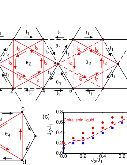
Figure 1:
(Color online) (a) and (b) The variational Ansatz with the NN hopping (black) and
NNN hopping (red) is shown. Solid (dashed) lines indicate positive (negative) hoppings,
which define the U(1) DSL. The phases and are added upon this Ansatz
to obtain a CSL. The direction of arrows indicates one possible convention of phases. In each up
and down triangle, the flux is ; in each hexagon the flux is .
The triangle has flux , and the triangle has flux
. (c) Phase diagram: the red dots (CSL) and blue squares (U(1) DSL) are the
calculated data. The red dashed line indicates the approximate phase boundary between the CSL and
U(1) DSL.
Method and Wave Function –
The variational wave functions are defined by the projected mean-field states:
(3)
where is the Gutzwiller projector,
which enforces no double occupation on each site. is the ground state of a
mean-field Hamiltonian that only contains hopping:
(4)
where () creates (destroys) an electron on site with
spin . Different spin-liquid phases can be described by the different patterns of
on the bonds of the lattice. Here, we consider the hoppings for nearest-neighbor (NN)
and next-nearest neighbor (NNN) bonds, indicated by and , respectively.
Since we are interested in CSL, we allow for both real and imaginary parts in the hopping i.e.,
. In Fig. 1, we show the Ansatz of our
variational wave function; since an orientation of the bond is needed:
for the hopping from to , () is taken in (opposite to) the direction
of the arrow.
Here, we choose the case where the up and down triangles have the same fluxes
(i.e., ), and the flux in the hexagon is .
This state can be represented as , as considered in Refs. ran,
and mei, . When including also the NNN bonds, a more complex flux structure appears in
the hexagon, as shown in Fig. 1: the triangles have flux
, and the triangles have flux .
Thus, the variational state can be represented by using the four fluxes () as
. The U(1) DSL, which has two Dirac point (for
each spin), has fluxes ; otherwise, the wave function describes a CSL. hastings
In our calculations, we set the real part of the NN hopping , and tune the imaginary
part to change . For each , we optimize the other two parameters (i.e.,
and ) using variational Monte Carlo to find the energetically favored state.
In particular, we use the stochastic reconfiguration (SR) optimization method, sorella
which allows us to obtain an extremely accurate determination of variational parameters.
Results –
We performed our variational calculations for the mean-field Hamiltonian Eq. (4)
at half filling on toric clusters with sites under the antiperiodic
boundary conditions (APBC), and compared the U(1) DSL and the CSL. We start from the U(1) DSL,
and add the fluxes gradually through increasing to get the CSL. If we only consider
the NN hopping term within the variational wave function, we find that, for ,
the CSL appears in the Heisenberg model as a local minimum. Most importantly,
only when the NNN term is taken into account, the CSL has an energy gain with respect to
the U(1) DSL. Therefore, in the following, we use the wave function including both and
.
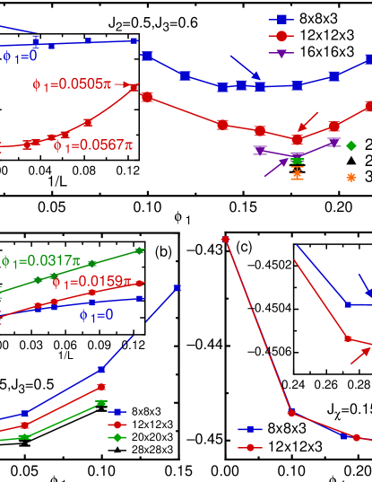
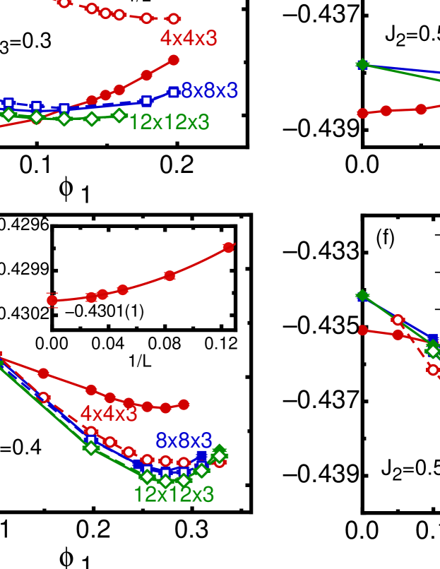
Figure 2:
(Color online) The energy per site as function of on different lattices. Results for the
Heisenberg model at with (a) and (b), for the
model at (c). Insets: the energy per site as function of for
the U(1) DSL () up to , and the CSL with on lattice
and on larger clusters up to (a); the finite size effect for different
(b) and with enlarged scale around (c). The arrows in (a) and (c)
show the energy minimum, and indicate the CSL stabilized in both models.
Our main results are presented in Fig. 2. For the
Heisenberg model of Eq. (1), we find that the CSL is energetically favored when
is a little larger than . As an example in Fig. 2(a), we show that,
at and , the energy exhibits a minimum at a finite value of , which
is for and for and . It is quite
time consuming to perform SR optimization on larger sizes, but, fortunately, the variational
parameters are only slightly modified from to (see supplemental material).
Therefore, we take the wave function optimized for to calculate variational energies up
to . After the finite-size scaling, which is shown in the inset of Fig. 2(a),
the estimated energy per site at and is . In this case, the
accuracy is about , compared with the DMRG data on cylinder geometries (where ).
By contrast, at and up to , the best energy is given by the U(1) DSL, see
Fig. 2(b). However, when we take the optimized wave functions at each and
perform the calculations up to , we find that the difference between the energies at
and is very small (i.e., of the order of ). Actually, performing
the finite size scaling yields the same estimated energy per site , as shown in the
insert of Fig. 2(b). This point is very close to the boundary of the phase transition,
thus it is hard to distinguish the CSL from the U(1) DSL. More results for different values of
and are shown in the supplemental material.
The rough phase diagram for the Heisenberg model is presented in
Fig. 1(c). Here, for , we get the CSL for , which is different
from the conclusion in Ref. mei, , which obtained . The reason of this
discrepancy might be due to the energy gain obtained by including the NNN hopping in the
variational wave function.
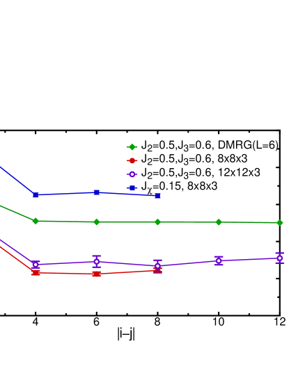
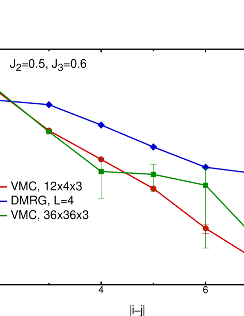
Figure 3:
(Color online) The chiral-chiral correlation function along direction on
and lattices for the Heisenberg model (at and ) and the
model (at ). The DMRG data are calculated on cylinder with
at and .
In order to detect the chiral order in the optimized wave functions, we measure the chiral-chiral
correlation function between two triangles defined as:
(5)
where is the chirality
of triangle . In Fig. 3, we show the chiral-chiral
correlation as a function of the distance between two
up triangles at and on and lattices.
On both clusters, decays rapidly to a finite value,
indicating the long-range chiral order, the difference between and being small.
It is interesting to note that the chiral order is larger in the accurate DMRG calculations
(performed cylinder with ) than in variational Monte Carlo ones.
The variational state with non-trivial fluxes ()
can be also implemented to the model of Eq. (2). In this case, the CSL is
stabilized much easier: even for a small value of , namely , there is
a clear minimum in the energy around , see Fig. 2(c).
For , the CSL has an energy per site , much lower than of the
U(1) DSL. Also the chiral-chiral correlation function in Fig. 3 indicates a robust
chiral order at .
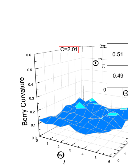
Figure 4:
(Color online) The Berry curvature at and on lattice. The Brillouin zone
is divided into a mesh with 100 plaquettes. The summation between and gives .
Until now, we have shown that the chiral state arises in these two models in view of the
chiral-chiral correlation. However, a CSL is further characterized by the non-trivial topological
structures, including the topological Chern number haldane and the degeneracy of the
ground state. wen1990 In the following, we proceed in these two directions to clarify
that our variational state indeed represents a CSL state.
First, the topological Chern number is computed as the integral over the Berry curvature
: niu1985 ; sheng2003 ; xwan ; hafezi
(6)
where (). To compute the Chern number numerically, we consider
twisted boundary conditions in the mean-field Hamiltonian, namely
and
. Then, we divide the
the Brillouin zone into plaquettes, with the Berry curvature being
(; for the four corners of the - plaquette, and
), where is the projected ground state of
the mean-field Hamiltonian with twisted boundary conditions. The overlap
is calculated by Monte Carlo method according to the weight
.
In order to numerically check the accuracy, we changed from 100 up to 400 plaquettes.
The numerical results show that the dimension of mesh changes the Berry curvature, but gives the same
topological Chern number. We must emphasize that the integration from to in the twist of
the fermionic operators includes two periods of phases for the spin operators and, therefore,
the result must be divided by . The integration between and gives with high
accuracy (see Fig. 4), leading to , which is fully consistent with recent DMRG
results. ssgong13
The degeneracy of the wave function, which indicates non-trivial ground-state structure, was not
obvious to obtain from the variational approach with the Gutzwiller projected parton
construction. Recently, Zhang et al.zhangyi realized that the ground-state
degeneracy is consistent with the linear dependence for variational wave functions through
fermionic construction for SU(2) Chern-Simons theory. We follow the same idea to construct the
linearly independent states from the four projected states that are obtained through changing
the boundary conditions of the mean field Hamiltonian in and
directions (see Fig. 1). We denote the four states as ,
where for periodic boundary condition and for antiperiodic boundary condition
(). In order to find the linearly independent states from these four projected states
(i.e., ), we calculate the overlaps
between all possible states. The numerical calculations up to indicate strong size effects,
due to the smallness of the mean-field gap. For example, for and on the
lattice with and , the band gap is only
about .
Thus, in order to suppress the finite-size effects on small clusters, we tune and
to enlarge the mean-field band gap (up to a value of ), still keeping the long-range chiral
order and a non-zero Chern number. Consequently, even on the small lattice, we
find the two linear independent states indicating the two-fold degeneracy,
which are (see the supplemental material for details):
(7)
(8)
Conclusions –
In conclusion, we investigated the CSL in the Heisenberg models on the Kagome
lattice by the variational approach with Gutzwiller projected fermionic construction. Our
variational studies reveal that the CSL is energetically favored in the phase region consistent
with the recent DMRG calculations. ssgong13 However, differently from the DMRG results,
we found that when is larger than , instead of , the CSL begins to appear
as indicated by the existence of energy minimum while tuning the fluxes.
On the other hand, we have shown that our wave function also works for the model,
which includes a three-spin parity and time reversal violating interaction.
Further investigations with these optimized wave functions show that the spin-spin correlation
functions decay fast (see supplemental material), indicating short-range correlations. Instead,
the chiral-chiral correlation function presents a long-range chiral order, consistent with DMRG
results. The variational wave function underestimates the robust of the CSL, as the accurate
DMRG calculations show stronger chiral order than variational state. Moreover, our calculations
of the topological Chern number and the ground state degeneracy suggest that the chiral state is
the Laughlin state.
Acknowledgements –
W.-J.H. and F.B. thank D. Poilblanc and Y. Iqbal for useful discussions.
This research is supported by the National Science Foundation through grants DMR-1408560 (W.-J.H,
D.N.S), DMR-1205734 (S.S.G.), and U.S. Department of Energy, Office of Basic Energy Sciences
under grant No. DE-FG02-06ER46305 (W.Z.). Y.Z. is supported by SITP. F.B. by PRIN 2010-11.
References
(1) L. Balents, Nature (London) 464, 199 (2010).
(2) X.-G. Wen, Phys. Rev. B 40, 7387 (1989); X.-G. Wen, Int. J. Mod. Phys. B 4, 239 (1990); X.-G. Wen and Q. Niu, Phys. Rev. B 41, 9377 (1990).
(3) P.A. Lee, Science 321, 1306 (2008).
(4) P. Mendels and F. Bert, J. Phys. Conf. Ser. 320, 012004 (2011).
(5) T.-H. Han, J. S. Helton, S. Chu, D. G. Nocera, J. A. Rodriguez-Rivera, C. Broholm, and Y. S. Lee, Nature 492, 406 (2012).
(6) J. Marston and C. Zeng, J. Appl. Phys. 69, 5962 (1991).
(7) M.B. Hastings, Phys. Rev. B 63, 014413 (2000).
(8) L. Balents, M.P.A. Fisher, and S.M. Girvin, Phys. Rev. B 65, 224412 (2002).
(9) F. Wang and A. Vishwanath, Phys. Rev. B 74, 174423 (2006).
(10) M. Hermele, Y. Ran, P.A. Lee, and X.-G. Wen, Phys. Rev. B 77, 224413 (2008).
(11) Y.-M. Lu, Y. Ran, and P.A. Lee, Phys. Rev. B 83, 224413 (2011); Y.-M. Lu, G. Y. Cho, and A. Vishwanath, arXiv: 1403.0575.
(12) L. Messio, B. Bernu, and C. Lhuillier, Phys. Rev. Lett. 108, 207204 (2012).
(13) Y. Ran, M. Hermele, P.A. Lee, and X.-G. Wen, Phys. Rev. Lett. 98, 117205 (2007).
(14) Y. Iqbal, F. Becca, and D. Poilblanc, Phys. Rev. B 84, 020407 (2011); Y. Iqbal, F. Becca, S. Sorella, and D. Poilblanc, Phys. Rev. B 87, 060405 (2013); Y. Iqbal, D. Poilblanc, and F. Becca, Phys. Rev. B 89, 020407 (2014).
(15) J.-W. Mei and X.-G. Wen, arXiv:1407.0869.
(16) H.C. Jiang, Z.Y. Weng, and D.N. Sheng, Phys. Rev. Lett. 101, 117203 (2008).
(17) S. Yan, D. Huse, and S. White, Science 332, 1173 (2011).
(18) S. Depenbrock, I.P. McCulloch, and U. Schollwck, Phys. Rev. Lett. 109, 067201 (2012).
(19) H.C. Jiang, Z. Wang, and L. Balents, Nat. Phys. 8, 902 (2012).
(20) S.S. Gong, W. Zhu, and D.N. Sheng, Scientific Reports 4, 6317 (2014).
(21) Y.C. He, D.N. Sheng, and Y. Chen, Phys. Rev. Lett. 112, 137202 (2014).
(22) B. Bauer, B.P. Keller, M. Dolfi, S. Trebst, and A.W.W. Ludwig, arXiv:1303.6963; B. Bauer, L. Cincio, B.P. Keller, M. Dolfi, G. Vidal, S. Trebst, and A.W.W. Ludwig, arXiv:1401.3017.
(23) V. Kalmeyer and R.B. Laughlin, Phys. Rev. B 39, 11879 (1989).
(24) X.-G. Wen, F. Wilczek, and A. Zee, Phys. Rev. B 39, 11413 (1989).
(25) K. Yang, L.K. Warman, and S.M. Girvin, Phys. Rev. Lett. 70, 2641 (1993).
(26) F.D.M. Haldane and D.P. Arovas, Phys. Rev. B 52, 4223 (1995).
(27) R.B. Laughlin, Phys. Rev. Lett. 60, 2677 (1988).
(28) F. Wilczek, Fractional Statistics and Anyon Superconductivity (World Science, Singapore, 1990).
(29) D.F. Schroeter, E. Kaplt, R. Thomale, and M. Grelter, Phys. Rev. Lett. 99, 097202 (2007).
(30) A.E.B. Nielsen, J.I. Cirac, and G. Sierra, Phys. Rev. Lett. 108, 257206 (2012).
(31) F. Wilczek and A. Zee, Phys. Rev. Lett. 52, 2111 (1984).
(32) R.B. Laughlin, Phys. Rev. Lett. 50, 1395 (1983).
(33) D. Arovas, J.R. Schrieffer, and F. Wilczek, Phys. Rev. Lett. 53, 722 (1984).
(34) X.-G. Wen, Phys. Rev. B 44, 2664 (1991).
(35) Y. Zhang, T. Grover, and A. Vishwanath, Phys. Rev. B 84, 075128 (2011); Y. Zhang, T. Grover, A. Turner, M. Oshikawa, and A. Vishwanath, Phys. Rev. B 85, 235151 (2012); Y. Zhang and A. Vishwanath, Phys. Rev. B 87, 161113 (2013).
(36) A.W.W. Ludwig, M.P.A. Fisher, R. Shankar, and G. Grinstein, Phys. Rev. B 50, 7526 (1994).
(37) S.S. Gong, W. Zhu, L. Balents, and D.N. Sheng, in preparation.
(38) S. Sorella, Phys. Rev. B 71, 241103 (2005).
(39) Q. Niu, D.J. Thouless, and Y.-S. Wu, Phys. Rev. B 31, 3372 (1985).
(40) D.N. Sheng, Xin Wan, E.H. Rezayi, Kun Yang, R.N. Bhatt, and F.D.M. Haldane, Phys. Rev. Lett. 90, 256802 (2003).
(41) X. Wan, D.N. Sheng, E.H. Rezayi, Kun Yang, R.N. Bhatt, and F.D.M. Haldane, Phys. Rev. B 72, 075325 (2005).
(42) M. Hafezi, A.S. Sorensen, M.D. Lukin, and E. Demler, Europhys. Lett. 81, 1005 (2008)
Supplemental Material
More energy data and spin-spin correlation functions —
We show the energy per site at different values of and with antiperiodic (APBC) and periodic (PBC)
boundary conditions in Fig. 5. On the lattice, the results depend on different
boundary conditions, owing to finite-size effect. As the size is increased to the lattice, the
energy per site only exhibits slight difference under different boundary conditions (of the order of ).
On larger clusters, the energy results with different boundary conditions are the same within one error bar.
The optimized values of the phases and for the wave functions with APBC and PBC are reported
in Table 1. By taking the wave functions optimized on the or
lattice, we perform variational calculations up to lattice, and perform the finite-size scaling
to obtain the estimated energies (see the insets of Fig. 5).
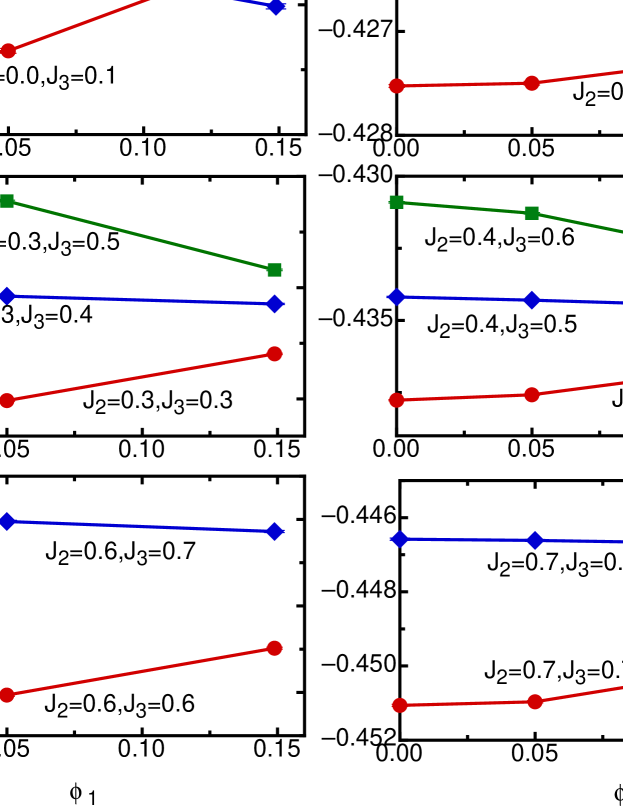
Fig. 6 shows several calculations on the lattice with APBC at different
and , qualitatively similar results are obtained with different boundary conditions. The CSL is energetically
favored when the energy per site decreases as the flux is increased. The schematic phase diagram shown
in the main text is constructed from these results.
Taking the optimized variational wave function on the lattice, we measure the spin-spin
correlation function, see Fig. 7 that also shows a comparison with DMRG results on cylinder with .
The fast decay of the spin correlation indicates the absence of a long-range order, consistent with DMRG conclusions.
Details for the degeneracy —
In order to find the linearly independent ground states, we numerically calculate all the overlaps between states
with different boundary conditions in the mean-field Hamiltonian, which are indicated by
.
In order to maximize the mean-field gap, i.e., , we take and
and perform the calculations on the lattice. By fixing the global phases in such a way
that all the overlaps with are real, we get the overlap matrix : zhangyi
(13)
(18)
(23)
The independent ground states can be found by diagonalizing the overlap matrix, i.e., .
We find that only two eigenvalues are non-zero, indicating that only two eigenvectors are linearly independent.
This fact implies that the ground-state degeneracy is two-fold. In particular, these two states can be constructed
such to preserve lattice symmetries. For example, we can consider the rotations, generated by the operator
. Within the Gutzwiller projected fermionic representation, the four wave functions from different boundary
conditions have the following relations under rotations:
Eigenstates of can be easily constructed, with eigenvalues , , and
:
Our numerical results of Eq. (13) imply that only two linearly independent states exist:
(24)
(25)
(26)
(27)
Therefore, the four projected states can be represented by using the two independent
states and :
Relation between the ground states and the minimum entropy states —
In this part, we want to find the relation between the two linearly independent states and of
Eqs. (24) and (25) and the minimum entropy states (MESs). zhangyi The MESs are the useful
basis of the degenerate ground-state manifold for topological ordered phases and label the eigenstates with different
quasiparticles threaded through the non-contractible loop along a given direction. The transformation between the
MES bases along different directions connected by a symmetry rotation is encoded in the corresponding modular
matrix. zhangyi
Since the Kagome lattice is symmetric under rotation and the topological order involve no
symmetry breaking, the overall ground-state manifold is invariant under . Nevertheless, each individual ground
state may still transform differently under , which can be interpreted as a conformal transformation:
,
where
are three directional vectors along the Bravais lattice vectors.
Therefore, on the Kagome lattice, the rotation leads to the modular transformation on
MESs. zhangyi For the CSL phase (e.g., the Laughlin state), we have the modular matrix:
(30)
(33)
where the phase factor in the definition of is given by the chiral edge central charge. The first and
the second columns (rows) are the identity particle and the semion quasi-particle, respectively. Physically, for Abelian
topological orders, the modular matrix determines the mutual statistics of a given quasi-particle encircling
around another one, while the modular matrix contains the self-statistics of the each quasi-particle.
With the modular matrix as the rotation operator, we can obtain the MESs along the
and directions and in terms of the MESs along
the direction , i.e., and
. Similarly, we can construct the other set of MESs ,
, and :
MES direction
Since under rotations, , and
, we may construct its eigenstates as the following:
(34)
(35)
(36)
which are consistent with the requirement that the ground states are only two-fold degenerate (similar results are
obtained by using ).
From Eqs. (24), (25), (34), and (35), we have that:
Figure 5:
(Color online) The energy per site on different lattices. The finite-size scaling and different flux is shown for
(a) and (b). Energy per site as a function of for different values of and
are reported in (c), (d), (e), and (f), for various sizes of the cluster: (red circles),
(blue squares), (green diamonds), and (black stars).
The filled (empty) points with solid (dashed) lines indicate APBC (PBC). The insets show the finite size scaling.
Table 1:
We list the fluxes and from the best chiral states in Fig. 5 for different
values of and on different sizes with APBC and PBC.
Figure 6:
(Color online) The energy per site at different and on the lattice. A CSL is energetically favored
when the energy per site shows a minimum as a function of .Figure 7:
(Color online) The spin-spin correlation function along the direction for and is shown for the
variational Monte Carlo (VMC) and density-matrix renormalization group (DMRG) calculations.