Making sense of the local Galactic escape speed estimates in direct dark matter searches

Abstract

Direct detection (DD) of dark matter (DM) candidates in the $\lesssim$10 GeV mass range is very sensitive to the tail of their velocity distribution. The important quantity is the maximum WIMP speed in the observer’s rest frame, i.e. in average the sum of the local Galactic escape speed $v_{\rm esc}$ and of the circular velocity of the Sun $v_{c}$. While the latter has been receiving continuous attention, the former is more difficult to constrain. The RAVE Collaboration has just released a new estimate of $v_{\rm esc}$ (Piffl et al., 2014 — P14) that supersedes the previous one (Smith et al., 2007), which is of interest in the perspective of reducing the astrophysical uncertainties in DD. Nevertheless, these new estimates cannot be used blindly as they rely on assumptions in the dark halo modeling which induce tight correlations between the escape speed and other local astrophysical parameters. We make a self-consistent study of the implications of the RAVE results on DD assuming isotropic DM velocity distributions, both Maxwellian and ergodic. Taking as references the experimental sensitivities currently achieved by LUX, CRESST-II, and SuperCDMS, we show that: (i) the exclusion curves associated with the best-fit points of P14 may be more constraining by up to $\sim 40$% with respect to standard limits, because the underlying astrophysical correlations induce a larger local DM density; (ii) the corresponding relative uncertainties inferred in the low WIMP mass region may be moderate, down to 10-15% below 10 GeV. We finally discuss the level of consistency of these results with other independent astrophysical constraints. This analysis is complementary to others based on rotation curves.

I Introduction

Direct detection (DD) of dark matter (DM) Goodman and Witten (1985); Drukier et al. (1986) has reached an impressive sensitivity thanks to developments in background rejection, increase in the target masses, and also boosted by the advent of dual-phase xenon detectors Angle et al. (2008); Ahmed et al. (2009); CDMS II Collaboration et al. (2010); Armengaud et al. (2011); Agnese et al. (2013); Aprile et al. (2013); Akerib et al. (2014). Weakly interacting massive particle (WIMP) candidates Primack et al. (1988); Jungman et al. (1996); Bergström (2000, 2009) are the main focus of such searches. In the last decade and half, important theoretical and experimental efforts have been invested in the inspection of the signal reported by the DAMA and DAMA/LIBRA Collaborations Bernabei et al. (2000, 2013), an annual modulation of the event rate possibly consistent with a WIMP signal Freese et al. (1988). Although some experiments have reported signal-like events in the light WIMP mass region $\sim 10$ GeV that might be consistent with the DAMA signal Aalseth et al. (2011); Angloher et al. (2012); Aalseth et al. (2013); Agnese et al. (2013), while not statistically significant, other negative results Agnese et al. (2014a); Akerib et al. (2014); CRESST Collaboration et al. (2014) tend to rule out the simplest interpretation in terms of spin-independent (SI) scatterings of WIMPs on nuclei. It also turns out that this WIMP mass range is not favored by indirect searches in the antiproton channel if the relic abundance is set by an s-wave annihilation to quarks Lavalle (2010); Cerdeno et al. (2012). Nevertheless, although the signal-like features show up very close to the experimental thresholds, and while there are some attempts to provide explanations of the DAMA signal in terms of backgrounds Pradler and Yavin (2013); Pradler et al. (2013); Davis (2014), a careful investigation of the phenomenology of light WIMPs is still worth it. We also note that this mass range has serious theoretical motivations from the model-building point of view (e.g. Refs. Bœhm and Fayet (2004); Kappl et al. (2011); Ellwanger and Hugonie (2014)).

The experimental sensitivity to light WIMPs strongly depends on both instrumental and astrophysical effects. The former is mostly related to the energy threshold and resolution of the detector, for given target nuclei and assuming perfect background rejection. The latter is related to the tail of the WIMP speed distribution function (DF) in the observer’s rest frame, as a detection threshold energy converts into larger speed thresholds for lighter WIMPs. The (annual average of the) maximum speed a WIMP can reach in the laboratory is the sum of the escape speed $v_{\rm esc}$, i.e. the speed a test particle would need to escape the Galactic gravitational potential at the Sun’s location, and of the circular velocity of the Sun. These are the two main astrophysical parameters relevant to assess the experimental sensitivity in the low WIMP mass regime. The latter is continuously investigated, and many studies have been revisiting and improving its estimation since the recommendation of 220 km/s by Kerr and Lynden-Bell Kerr and Lynden-Bell (1986). As for $v_{\rm esc}$, which should be a real physical cutoff in the velocity DF of the gravitationally bound WIMPs as measured in the dark halo rest frame, constraints are more scarce. Better understanding and better estimating the escape speed should therefore strongly benefit direct searches for light WIMP candidates.

The local Galactic escape velocity can be estimated with different approaches. One can go through a global halo modeling from photometric and kinematic data (e.g. Refs. Catena and Ullio (2010); McMillan (2011)) and compute the gravitational potential from the resulting mass model. This is an indirect estimate that mostly relies on rotation curve fitting procedures. A more direct estimate consists of trying to use those nearby high-velocity stars which are supposed to trace the tail of the corresponding stellar phase-space DF, which, though not necessarily equal to the DM DF, should still also vanish at the escape speed. Ideally, both kinds of estimate should converge, which would mean that the global dynamics is well understood and well modeled, and that the selected data are indeed sensible and relevant tracers. A few studies have pushed in the latter direction since the seminal work by Leonard and Tremaine Leonard and Tremaine (1990). In particular, two results have been published based on the data of the RAVE survey, a massive spectroscopic survey of which the first catalog was released in 2006 Steinmetz et al. (2006). One of these results was based upon the first data release Smith et al. (2007) (hereafter S07), and provided an estimate of $\mbox{$v_{\rm esc}$}=544^{+64}_{-46}$ at 90% confidence level (CL). This value is now used in the so-called standard/simplest halo model (SHM), a proxy for the local DM phase-space conventionally employed to derive DD exclusion curves (see e.g. Ref. McCabe (2010) for associated uncertainties). The latest RAVE analysis, which relies on the fourth data release and different assumptions, was published in 2014 Piffl et al. (2014a) (hereafter P14) and found $\mbox{$v_{\rm esc}$}=533^{+54}_{-41}$ at 90% CL, consistent with the previous result while slightly reducing the central value and the statistical errors (consistent with yet another even more recent study Kafle et al. (2014)). Among improvements with respect to S07, P14 used much better distance and velocity reconstructions, and a more robust star selection. This means that systematic errors should have decreased significantly. We will focus on this result in the following.

Whereas it is straightforward to derive the impact of this new escape speed range on the exclusion curves or signal contours, or to include it as independent constraints or priors in Bayesian analyses, it is worth stressing that this would lead to inconsistent conclusions in most cases, as, in particular, the range itself relies on a series of assumptions. In this paper, we will examine these assumptions and derive self-consistent local DM phase-space models, accounting for correlations in the astrophysical parameters. We will see that these correlations translate into DD uncertainties quite different from those that would be obtained by using the 90% CL range blindly, and even lead to slightly more stringent DD limits than in the standard derivation.

Although the way astrophysical parameters affect direct detection searches is rather well understood (e.g. Refs. Green (2010, 2012); Freese et al. (2013)), the related uncertainties are still to be refined. A consensual method to determine and reduce these uncertainties is essentially based upon building a Galactic mass model constrained from observational data. The issue is then twofold: (i) describe the Galactic content (baryons and DM) as consistently as possible and (ii) use the observational constraints as consistently as possible. There have been several studies mostly based on rotation curves and on local surface density measurements which tried to bracket the astrophysical uncertainties (e.g. Refs. Arina et al. (2011); Catena and Ullio (2012); Fairbairn et al. (2013); Bozorgnia et al. (2013)), and where essentially point (i) was brought to the fore. Here, we provide a complementary view focusing on constraints that rely on different observables, namely non corotating high-velocity stars, with emphasis on the escape speed. We will adopt the same global method as previous references (namely use a Galactic mass model), but will rather put the emphasis on point (ii). Concentrating on the escape speed is particularly relevant to light WIMP searches.

The outline of this paper is the following. We will first review the results obtained in Ref. Piffl et al. (2014a) (P14) and derive a local DM phase-space DF consistent with their assumptions. Then, thanks to this phase-space modeling, we will convert their 90 and 99% CL ranges into uncertainties in DD exclusion curves. We will eventually discuss these results in light of other complementary and independent astrophysical constraints before concluding.

II Local DM phase space from RAVE P14 assumptions and results

II.1 Brief description of RAVE P14 and main parameter assumptions

The RAVE-P14 analysis is based on a sample of stars from the RAVE catalog which are not corotating with the Galactic disk (34 or 69 stars after selection cuts, mostly hard ($>300$ km/s) or weak ($>200$ km/s) velocity cut, respectively. It is complemented with data from another catalog Beers et al. (2000), which were used to derive the best-fit range for the escape speed recalled above (19 or 17 stars). Therefore, the full sample contains high-velocity halo stars which are assumed to probe the high-velocity tail of the phase-space DF. We will only consider results obtained with a hard velocity cut in the following.

Assuming steady state and that the phase-space DFs of DM and non corotating stars mostly depends on energy, one may introduce the concept of escape speed $v_{\rm esc}$  by stating that the phase-space DF must vanish for speeds greater than $\mbox{$v_{\rm esc}$}(\vec{x})=\sqrt{-2\,\phi(\vec{x})}$ (consistently with Jeans theorem), where $\phi(\vec{x})$ is the gravitational potential at position $\vec{x}$ (e.g. Ref. Binney and Tremaine (2008)). Then, observational constraints on $v_{\rm esc}$ from stellar velocities can only be derived if the true shape of the underlying velocity DF is known. P14 used the Ansatz proposed in Ref. Leonard and Tremaine (1990) for the high-velocity tail of the DF of stars, which reads $f(v)\propto(\mbox{$v_{\rm esc}$}-v)^{k}\,\theta(\mbox{$v_{\rm esc}$}-v)$, where $v=|\vec{v}|$ and $k$ is a free index calibrated from galaxy simulations. This Ansatz is general enough and holds provided $v$ is close to $v_{\rm esc}$. It differs from the one used in S07, $f(v)\propto(v_{\rm esc}^{2}-v^{2})^{k}\,\theta(\mbox{$v_{\rm esc}$}-v)$. Actually, P14 tested both Ansätze with cosmological simulations performed in Ref. Scannapieco et al. (2009), which include baryons and star formation, and found the former to be more consistent with the simulation results—note that S07 also employed cosmological simulations, though less recent, to calibrate their reconstruction method. This is a significant systematic difference between S07 and P14, though the quantitative impact is not spectacular; when performing their likelihood analysis from the S07 Ansatz, P14 find $\mbox{$v_{\rm esc}$}=537^{+37}_{-33}$ km/s instead of their nominal result $\mbox{$v_{\rm esc}$}=533^{+54}_{-41}$ (90% CL).

Another systematic difference between S07 and P14 likelihood analyses, which allows the latter to increase statistics, is that P14 applied a correction to the selected star velocities to “relocate” them at the radial position of the Sun $r_{\odot}$ before running their likelihood. Given a line-of-sight velocity component $v_{||}(\vec{x})$ for a star located at position $\vec{x}$, the correction reads $v_{||}^{\prime}(\vec{x}_{\odot})=v_{||}(\vec{x})\times\sqrt{|\phi(\vec{x}_{\odot})/\phi(\vec{x})|}$, where $\vec{x}_{\odot}$ is the position of the Sun and $\phi$ is the total gravitational potential. These corrected speeds are supposed to describe the local DF more reliably and are expected to reduce the systematic uncertainties in the determination of $v_{\rm esc}$, while increasing the statistics.

S07 actually dealt with that issue by selecting stars within a small radial range centered around $r_{\odot}$, but from more recent distance estimates, it turns out that their sample is likely biased (see the discussion in P14). We may remark that, despite the improvements in the P14 methodology with respect to S07, correcting the star velocities by the gravitational potential automatically introduces a Galactic mass model dependence. Even though the gravitational potential is not expected to vary much for nearby stars, this aspect is important when one wants to use P14 results in the context of DD. We will show how to cope with that in the next (sub)sections.

Before going into the details of the Milky Way (MW) mass modeling, it is worth recalling some key parameters that are used in P14. First, $r_{\odot}$ is fixed to the central value found in Ref. Gillessen et al. (2009),

$$\mbox{$r_{\odot}$}=8.28\;{\rm kpc}\,.$$ (1)

For the circular velocity of the Sun, $v_{c}$, three cases were considered, each associated with different results for $v_{\rm esc}$: (i) 220 km/s, (ii) 240 km/s, and (iii) free $v_{c}$ — we will discuss these cases in more details later on. Finally, the peculiar velocity of the Sun was fixed to the vector elements found in Schönrich et al. (2010):

$$U_{\odot} = 11.1\;{\rm km/s}$$ (2)

$$V_{\odot} = 12.24\;{\rm km/s}$$

$$W_{\odot} = 7.25\;{\rm km/s}\,.$$

II.2 Milky Way mass model

Since P14 likelihood relies on star relocation, a procedure in which measured stellar speeds are corrected by the gravitational potential, the escape speed estimate must be used consistently with the Galactic mass model they assumed. The latter is made of three components: a dark matter halo, a baryonic bulge, and a baryonic disk. We note that the baryonic content is fixed, while the DM halo parameters are left free for the P14 likelihood analysis. There is therefore a direct correlation between the dark halo parameters and the escape speed as a result of P14 analysis.

The baryonic bulge is described with a spherical Hernquist density profile Hernquist (1990) as

$$\rho_{\rm b}(r)=\frac{M_{\rm b}}{2\,\pi}\frac{r_{\rm b}/r}{(r+r_{\rm b})^{3}}\,,$$ (3)

where $r$ denotes the Galactocentric radius, $G$ is Newton’s constant, $r_{\rm b}$ is a scale radius, and $M_{\rm b}$ is the total bulge mass. The parameter values are given in Table 1. To this profile is associated a gravitational potential:

$$\phi_{\rm b}(r) =-G\frac{M_{\rm b}}{(r+r_{\rm b})}\,.$$ (4)

The disk is modeled from an axisymmetric Miyamoto–Nagai profile Miyamoto and Nagai (1975),

$$\rho_{\rm d}(R,|z|)=z_{\rm d}^{2}\,\frac{M_{\rm d}}{4\,\pi}\,\left\{\frac{R_{\rm d}R^{2}+(R_{\rm d}+3\sqrt{z^{2}+z_{\rm d}^{2}})(R_{\rm d}+\sqrt{z^{2}+z_{\rm d}^{2}})^{2}}{\left[R^{2}+(R_{\rm d}+\sqrt{z^{2}+z_{\rm d}^{2}})^{2}\right]^{5/2}(z^{2}+z_{\rm d}^{2})^{3/2}}\right\},$$ (5)

where $M_{\rm d}$ is the total disk mass and $R_{\rm d}$ and $z_{\rm d}$ are radial and vertical scale lengths. The parameter values are given in Table 1. This profile converts into the following potential:

$$\phi_{\rm d}(R,|z|)=-G\frac{M_{\rm d}}{\sqrt{R^{2}+(R_{\rm d}+\sqrt{z^{2}+z_{\rm d}^{2}})^{2}}}\;.$$ (6)

Finally, the DM halo was modeled from a spherical NFW profile Navarro et al. (1997),

$$\rho(r)=\rho_{s}\,x^{-1}\,(1+x)^{-2}\,,$$ (7)

where $x=r/r_{s}$, and $\rho_{s}$ and $r_{s}$ are a scale density and a scale radius, respectively, which are left as free parameters in P14. The associated gravitational potential reads:

$$\phi_{\rm dm}(r) = -4\,\pi\,G\,\frac{\rho_{s}\,r_{s}^{3}}{r}\,\ln\left(1+\frac{r}{r_{s}}\right)$$

$$\underset{r\to 0}{\longrightarrow} -4\,\pi\,G\,\rho_{s}\,r_{s}^{2}\,,$$

which is minimal and finite at the Galactic center as shown by the limit above. Note that P14 also considered an adiabatically contracted NFW, but we will not discuss this case here.

Actually, P14 mostly used the concentration parameter $c$ and the total Milky Way mass instead of $r_{s}$ and $\rho_{s}$, which is strictly equivalent. The former is defined as

$$c_{340}=\frac{R_{340}}{r_{s}}\,,$$ (9)

where $R_{340}$ is the radius that encompasses the DM halo such that the average DM density is 340 times the critical density $\rho_{c}$ (taking a Hubble parameter of $H_{0}=73$ km/s/Mpc):

$$R_{340}=\left(\frac{3\,M_{\rm dm}(R_{340})}{4\,\pi\times 340\,\rho_{c}}\right)^{1/3}\,.$$ (10)

Here, $M_{\rm dm}$ is the full dark matter mass enclosed within a radius of $R_{340}$. The total Milky Way mass $M_{340}$ is defined as the sum of the DM and baryonic components inside $R_{340}$,

$$M_{340}=M_{\rm tot}(R_{340})=M_{\rm dm}(R_{340})+M_{\rm b}+M_{\rm d}\;.$$ (11)

Baryonic component	Total mass	Scale parameters
Bulge	$M_{\rm b}=1.5\times 10^{10}$$M_{\odot}$	$r_{\rm b}=0.6$ kpc
Disk	$M_{\rm d}=5\times 10^{10}$$M_{\odot}$	$R_{\rm d}=4$ kpc $z_{\rm d}=0.3$ kpc

Table 1: Values of the parameters associated with the baryonic components of the mass model.

II.3 Circular and escape speeds: Converting the original RAVE P14 results

The MW mass model defined in the previous section is used to connect the RAVE data, i.e. the stellar line-of-sight velocities, to the circular velocity $v_{c}$ in the MW disk ($z=0$) at the position of the Sun. Indeed, from classical dynamics, the circular velocity $v_{c}$ in the MW disk ($z=0$) is related to the radial gradient of the gravitational potential,

$$v_{c}^{2}(R,z=0)=R\,\partial_{R}\phi_{\rm tot}(R,z=0)\,,$$ (12)

where the expression is given in its axisymmetric form ($r^{2}=R^{2}+z^{2}$), and where $\phi_{\rm tot}$ is the sum of all contributions to the gravitational potential (baryonic components and DM). At distance $r_{\odot}$, one has therefore

$$v_{c}^{2}(\mbox{$r_{\odot}$},z=0)=\mbox{$r_{\odot}$}\,G\,\left\{\frac{M_{\rm b}}{(\mbox{$r_{\odot}$}+r_{\rm b})^{2}}+\frac{\mbox{$r_{\odot}$}\,M_{\rm d}}{(r_{\odot}^{2}+\bar{R}_{\rm d}^{2})^{3/2}}+4\,\pi\,\frac{\rho_{s}\,r_{s}}{x_{\odot}^{2}}\left(\ln(1+x_{\odot})-\frac{x_{\odot}}{1+x_{\odot}}\right)\right\}\,,$$ (13)

where $\bar{R}_{\rm d}=R_{\rm d}+z_{\rm d}$. In P14, three different choices were made for $v_{c}$: 220 km/s, 240 km/s, and free parameter for the likelihood. In the last case, the best fit to the data is obtained for $v_{c}=196$ km/s, a value significantly smaller than most recent estimates (e.g. Refs. Schönrich (2012); Reid et al. (2014)). Nevertheless, this fit includes a prior on the concentration parameter based on Ref. Macciò et al. (2008), which strongly affects the result (the best-fit obtained for the concentration is $c_{340}=5$). We will discuss this in more details in Sec. III.4.

Figure 1: P14 likelihood results converted in the plane $v_{\rm esc}$-$v_{c}$. See text for details.

We now come to the main observable constrained in P14: the escape speed at the solar location. It is in principle defined from the global gravitational potential at the position of the Sun, as $v_{\rm esc}=\sqrt{-2\,\phi_{\rm tot}(\mbox{$r_{\odot}$})}$. Nevertheless, even though the potential is usually assumed to vanish at infinity, the presence of nearby galaxies such as Andromeda, located at $\sim 790$ kpc Stanek and Garnavich (1998); Riess et al. (2012), makes it tricky to define the potential difference relevant to the escape. As an educated guess, P14 assumed a boundary

$$R_{\rm max}=3\,R_{340}\,,$$ (14)

which roughly lies in the range 500-600 kpc. Accordingly, the escape speed is defined from the (positive) potential difference $\psi$ such that

$$\mbox{$v_{\rm esc}$}(\mbox{$r_{\odot}$}) \equiv \sqrt{2\,\psi_{\rm tot}(\mbox{$r_{\odot}$})}\,,$$ (15)

$$\psi_{\rm tot}(\mbox{$r_{\odot}$}) \equiv -\left(\phi_{\rm tot}(\mbox{$r_{\odot}$})-\phi_{\rm tot}(R_{\rm max})\right)\,.$$ (16)

While $\psi_{\rm tot}$ contains all matter components, this definition will also be retained for individual components.

Since the baryonic MW mass model components are fixed, a pair of ($v_{c},\mbox{$v_{\rm esc}$}$) directly converts into a pair of NFW parameters ($\rho_{s},r_{s}$), or equivalently ($M_{340},c_{340}$). Actually, the likelihood function in P14 uses $v_{c}$ and $v_{\rm esc}$ as input variables, while the results for the $v_{c}$-free case (no prior on $v_{c}$) have been illustrated in the $M_{340}$-$c_{340}$ plane (see Fig. 13 in P14). For the latter case, we have used Eqs. (13) and (15) to convert the results back in the plane $v_{\rm esc}$-$v_{c}$, more relevant to derive uncertainties in direct detection, as it will be discussed in Sec. III.

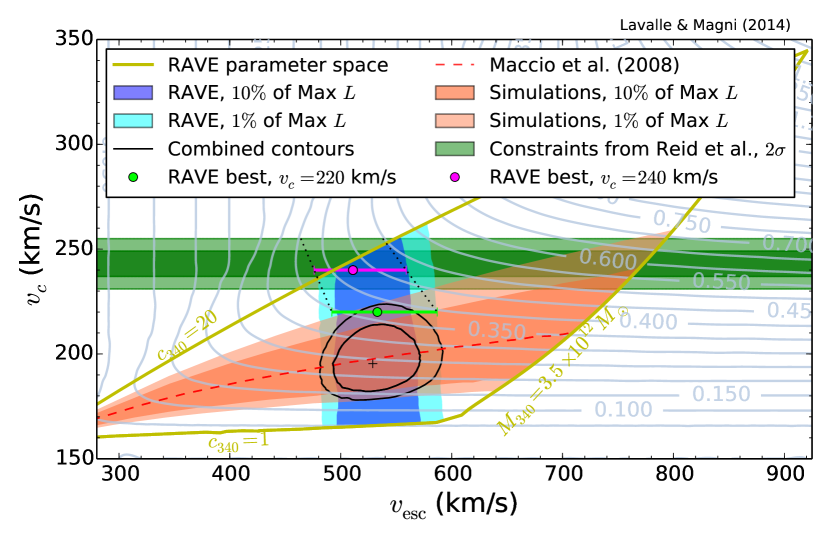
We summarize P14 results in Fig. 1, in the plane $v_{\rm esc}$-$v_{c}$. P14 best-fit values of $v_{\rm esc}$ obtained after enforcing $v_{c}=$ 220 (240) km/s —no prior on concentration— are shown as green (magenta) points, with associated 90% CL errors (these points are taken from Table 3 in P14). Then we report the P14 results obtained in the $v_{c}$-free case, which were originally shown in the $M_{340}$-$c_{340}$ plane (their Fig. 13, left panel). The original frame of Fig. 13 in P14 is reported as the yellowish curves. The 10% (1%) of the maximum likelihood band is shown as the dark (light) blue area, while the 90% (99%) CL log-normal prior on the concentration parameter appears as a dark (light) orange band, and the concentration model of Ref. Macciò et al. (2008) is displayed as a dashed red curve. The final contours accounting for the concentration prior is shown as black curves. Besides, we have also calculated and reported the iso-DM-density curves (gray lines) at the solar location, $\rho_{\odot}=\rho(\mbox{$r_{\odot}$})$, in units of GeV/cm³. Finally, the green band shows additional constraints on $v_{c}$ taken from Ref. Reid et al. (2014) that we will discuss in Sec. III.3.

We must specify that the 1 and 10% of maximum likelihood characterizing uncertainty bands in Fig. 1 are formally defined in the plane $M_{340}$-$c_{340}$, so there is a priori no reason as to why these bands should be representative of a meaningful probability range in the plane $v_{\rm esc}$-$v_{c}$. Nevertheless, this part of the P14 analysis still provides additional information with respect to the cases with priors on $v_{c}$, as it is supposed to leave $v_{c}$ as a free parameter. Since the 1% band fully encompasses the two best-fit points with priors $v_{c}=$220/240 km/s (the latter’s error slightly overshoots the 1% band), we may take it as roughly representative of a $\sim 90$% CL range in the plane $v_{\rm esc}$-$v_{c}$, even though the posterior PDFs associated with ($M_{340},c_{340}$) are different from the ones related to ($\mbox{$v_{\rm esc}$},v_{c}$). We may still grossly guess the relation between the posterior PDF $P$ for $M_{340}$ (marginalizing over $c_{340}$), and that for $v_{\rm esc}$, $\bar{P}$. Since we have the approximate scaling $v^{2}\sim M_{340}\,f(\mbox{$r_{\odot}$},c_{340})$, where $f$ is a function that would become constant after marginalization (this relation holds for both $v_{\rm esc}$ and $v_{c}$, and would only differ in the definition of $f$), then $P(M_{340})dM_{340}\sim P(M_{340}(v))\,v\,dv$, such that $\bar{P}(v)\sim v\,P(M_{340}(v))$. Therefore, we may expect a longer tail in $v$-space. Interestingly, we see that the offset between the 1% band and the 220 km/s point is consistent with this rough expectation (while not the 240 km/s point, likely because the data-induced $v_{c}$-$v_{\rm esc}$ anticorrelation was not included in the $v_{c}$-free analysis of P14, which was instead calibrated from the 220 km/s point — see discussion below).

We clearly see from Fig. 1 that the P14 results, because of the initial assumptions, induce strong correlations among the local DM parameters relevant to predictions in direct DM searches. Therefore, a blind use of the escape velocity constraints, as very often done (e.g. by taking arbitrary values of local DM density), can already be classified as inconsistent. Fig. 1 will be our primary tool to make a consistent interpretation of P14 results in the frame of direct DM detection.

We may also note that the trend of the blue band is in contrast with the claim in P14 that the authors’ $v_{\rm esc}$ estimate anticorrelates with $v_{c}$ as a result of their sample selection (biased to negative longitudes), which explains why $v_{\rm esc}$ decreases from 533 to 511 km/s as $v_{c}$ increases from 220 to 240 km/s — we have illustrated this anticorrelation in Fig. 1 with dotted lines. This actually comes from the method used in P14 to extract the likelihood region in the $c_{340}$-$M_{340}$ plane (see their Fig. 13): the authors kept the posterior PDF of $v_{\rm esc}$ frozen to the shape obtained with $v_{c}=220$ km/s, while varying only $c_{340}$ and $M_{340}$. This means that they did not recompute the velocities of their stellar sample according to the changes in $v_{c}$ induced by those in $c_{340}$ and $M_{340}$. Such an approximation is hard to guess from the text, and is even more difficult from their Fig. 13 showing the likelihood band in the $c_{340}$-$M_{340}$ plane. Indeed, they also report iso-$v_{c}$ curves on the same plot, so we may expect that the corresponding posterior PDF for $v_{\rm esc}$ was taken accordingly. We remind the reader that in principle the pair $v_{c}$-$v_{\rm esc}$ is strictly equivalent to the pair $c_{340}$-$M_{340}$, so we may have expected to recover the anticorrelation claimed for the former pair from the contours obtained for the latter. While the goal of P14 in the $v_{c}$-free case was mostly to investigate how to improve the matching between Galactic models and the primary fit results, with a focus on the Milky Way mass, this somehow breaks the self-consistency of the analysis. This has poor impact on the Galactic mass estimate, which was the main focus in P14, but this affects the true dynamical correlation that $v_{\rm esc}$ should exhibit with the other astrophysical parameters. Unfortunately, improving on this issue would require access to the original data, which is beyond the scope of this paper. Therefore, we will stick to this result in the following, and further comment on potential ways to remedy this limitation at the qualitative level in Sec. III.4.2.

To conclude this section, we calculate and provide in Table 2 the DM halo parameters associated with the P14 best-fit points. We stress that to each value of $v_{\rm esc}$ found in the table corresponds a specific value of the local DM density. This kind of correlations should be taken into account for a proper use of P14 results. It is obvious that the relevance of the values and ranges for these parameters should be questioned in light of complementary constraints. We will discuss this issue in Sec. III.4.

Model assumptions	$v_{c}$	$v_{\rm esc}$	$\rho_{s}$	$r_{s}$	$\rho_{\odot}$
	(km/s)	(km/s)	(GeV/cm3)	(kpc)	(GeV/cm3)
Prior $v_{c}=220$ km/s	220	$533^{+54+109}_{-41-60}$	$0.42^{+0.26+0.48}_{-0.16-0.24}$	$16.4^{+6.6+13.6}_{-4.5-6.4}$	$0.37^{+0.02+0.04}_{-0.03-0.04}$
Prior $v_{c}=240$ km/s	240	$511^{+48}_{-35}$	$1.92^{+1.85}_{-0.82}$	$7.8^{+3.8}_{-2.2}$	$0.43^{+0.05}_{-0.05}$
$v_{c}$ free	$196^{+26}_{-18}$	$537^{+44}_{-55}$	$0.08^{+0.31}_{-0.07}$	$36.7^{+50.7}_{-19.0}$	$0.25^{+0.14}_{-0.12}$

Table 2: Values of the DM halo parameters associated with P14 best-fit points. The reported errors correspond to 90% CL and 99% CL, the latter being inferred from the PDFs reported in Fig. 11 in P14. The 99%CL cannot be inferred for the “$v_{c}=240$ km/s” case from P14. For the “$v_{c}$-free” case, the errors are taken from Fig. 13 of P14, and roughly correspond to 90% CL — see also Fig. 1 of this paper. See the text for further details.

III Uncertainties in direct DM searches

In this section, we sketch a method to make a self-consistent interpretation of P14 results, and show how they convert into astrophysical uncertainties beyond only uncertainties in the escape speed. We will explicitly show the impact of dynamical correlations between the local circular and escape speeds and the DM parameters.

III.1 Generalities

We recall here the main equations and assumptions used to make predictions in direct DM searches, focusing on the spin-independent class of signals (reviews can be found in e.g. Refs. Lewin and Smith (1996); Jungman et al. (1996); Freese et al. (2013)). Assuming elastic collisions between WIMPs of mass $m_{\chi}$ and atomic targets of atomic mass number $A$ and mass $M$ (and equal effective couplings $f_{n}$ and $f_{p}$ of WIMPs to neutrons and protons), the differential event rate per atomic target mass in some DD experiment reads

$$\frac{dR}{dE_{\rm r}}=\frac{\rho_{\odot}}{\mbox{$m_{\chi}$}}\,\frac{A^{2}\,\sigma_{p}\,F^{2}(q)}{2\,\mu_{p}^{2}}\,\eta(v_{\rm min}(E_{\rm r}),t)\,,$$ (17)

where $\mu_{p}$ is the WIMP-proton reduced mass, $q$ is the exchanged momentum, $E_{\rm r}=q^{2}/(2\,M)$ is the nuclear recoil energy, $\sigma_{p}=(4/\pi)\,\mu_{p}^{2}\,f_{p}^{2}$ is the WIMP-proton cross section, $F(q)$ is a nuclear form factor, and $\eta$ is the truncated mean inverse local WIMP speed beyond a threshold $v_{\rm min}$:

$$\eta(v_{\rm min}(E_{\rm r}),t)=\int_{v>v_{\rm min}}d^{3}\vec{v}\,\frac{f_{\oplus}(\vec{v},t)}{v}\,.$$ (18)

Here, $v=|\vec{v}|$ is the WIMP speed in the observer frame, and $f_{\oplus}$ is the associated DF (normalized to unity over the full velocity range). The threshold speed

$$v_{\rm min}(E_{\rm r},\mbox{$m_{\chi}$},M)=\sqrt{M\,E_{\rm r}/(2\,\mu^{2})}\,,$$ (19)

where $\mu$ is the WIMP-nucleus reduced mass, is the minimal speed to achieve a recoil energy of $E_{\rm r}$. A simple Galilean transformation allows one to connect the WIMP velocity DF in the local frame $f_{\oplus}$ to that in the Milky Way frame $f$:

$$f_{\oplus}(\vec{v},t)=f(\vec{v}+\vec{v}_{\oplus}(t))\,.$$ (20)

We will further discuss the form of $f$ in Sec. III.2. The time dependence is explicitly shown to arise from the Earth’s motion around the Sun $\vec{v}_{\oplus/\odot}(t)$, since the Earth’s velocity in the MW frame is given by $\vec{v}_{\oplus}(t)=\vec{v}_{\odot}+\vec{v}_{\oplus/\odot}(t)$. In a frame whose first axis points to the Galactic center and the second one in the direction of the rotation Galactic flow in the disk, we may parametrize the solar velocity as

$$\vec{v}_{\odot}=(U_{\odot},V_{\odot}+v_{c},W_{\odot})\,,$$ (21)

where $v_{c}$ is the circular speed and the peculiar components are given in Eq. (2). For the Earth motion around the Sun, featured by $\vec{v}_{\oplus/\odot}(t)$, we will use the prescription of Ref. Green (2003), the accuracy of which has been recently confirmed again in Refs. Lee et al. (2013); McCabe (2014).

To compute the event rate above a threshold for a given experiment, or more generally inside an energy bin (or interval) $i$, one has further to account for the experiment efficiency $\epsilon(E_{\rm r})$ and (normalized) energy resolution $G(E_{\rm r},E_{\rm r}^{\prime})$ such that:

$$R_{i}(t)=\int_{0}^{\infty}dE_{\rm r}\,\epsilon(E_{\rm r})\,\frac{dR(E_{\rm r})}{dE_{\rm r}}\int_{E_{i}^{\rm min}}^{E_{i}^{\rm max}}dE_{\rm r}^{\prime}\,G(E_{\rm r},E_{\rm r}^{\prime})\,.$$

(22)

A sum over the fractions of atomic targets must obviously be considered in case of multitarget experiments (or to account for several isotopes). To very good approximation, we can define the average and modulated rates, $\bar{R}_{i}$ and $\tilde{R}_{i}$ as

$$\bar{R}_{i} = \frac{1}{2}\left\{R_{i}(t_{\rm max})+R_{i}(t_{\rm min})\right\}$$ (23)

$$\tilde{R}_{i} = \frac{1}{2}\left\{R_{i}(t_{\rm max})-R_{i}(t_{\rm min})\right\}\,,$$ (24)

where $t_{\rm max}\simeq 152$ ($t_{\rm min}\simeq 335$) is the day of the year where the rate is maximum (minimum), which can revert in some cases depending on the WIMP mass for a given energy threshold (and vice versa).

One can read the trivial scaling in the local density $\rho_{\odot}$ off Eq. (17), which still helps understand the implication of a self-consistent use of P14 results. Indeed, we have seen in the previous section that $\rho_{\odot}$ was correlated with the circular speed $v_{c}$ as well as to the escape speed $v_{\rm esc}$ by construction. We investigate the impact of the velocity DF in the next subsection.

III.2 Toward consistent DM velocity distributions

Figure 2: Comparison between a truncated MB DF and an ergodic DF. Left panel: Assuming the parameters of the P14 best-fit point with $v_{c}=220$ km/s, we show the MB curve and several curves for ergodic case to make the impact of the baryonic components explicit. Right panel: Comparison of the MB-like DFs with the ergodic DFs assuming the parameters of the P14 best-fit points with both $v_{c}=220$ and 240 km/s. Here, we also show the DFs associated with the upper and lower corners of the 90%CL interval.

Here we shortly introduce the usual way to deal with the WIMP velocity DF before specializing to the ergodic assumption. A nice review can be found in Ref. Green (2012).

III.2.1 Standard halo model

Most of the DD limits or signal regions are derived by means of the so-called standard halo model (SHM), which is conventionally used to compare experimental sensitivities and results. Beside fixing the local DM density $\rho_{\odot}$, the SHM specifies the WIMP velocity distribution as a truncated Maxwell-Boltzmann (MB) distribution, based on the assumption of an isothermal sphere, and defined in the MW rest frame as:

$$f_{\rm MB}(\vec{v})=\begin{cases}N_{0}\,\left\{e^{-\frac{v^{2}}{v_{c}^{2}}}-e^{-\frac{v_{\rm esc}^{2}}{v_{c}^{2}}}\right\}\;\forall v\leq\mbox{$v_{\rm esc}$}\\ 0\;\forall v>\mbox{$v_{\rm esc}$}\end{cases}$$ (25)

where $N_{0}$ allows a normalization to unity over $d^{3}\vec{v}$, and the right-hand side term enforces the phase-space DF to vanish at $v_{\rm esc}$. The SHM is also sometimes defined with a hard velocity cutoff, which corresponds to neglecting the second term of the right-hand side above. As this function is here defined in the Galactic frame, a proper use in DD merely rests upon the Galilean transformation of Eq. (20).

The SHM is defined with fixed parameters that we summarize below:

$$\rho_{\odot}^{\rm shm} = 0.3\;{\rm GeV/cm^{3}}$$ (26)

$$v_{c}^{\rm shm} = 220\;{\rm km/s}$$

$$v_{\rm esc}^{\rm shm} = 544\;{\rm km/s}\,.$$

The escape speed value is actually the central value found in the first RAVE analysis, S07  Smith et al. (2007). It is noteworthy that the velocity dispersion relation

$$\sigma_{\rm MB}^{2}=3\,v_{c}^{2}/2$$ (27)

predicted from the Jeans equations in the absence of anisotropy for the isothermal sphere is no longer valid as soon as the by-hand truncation at $v_{\rm esc}$ is introduced. While the difference is quantitatively not important, especially for both low circular speed and large escape speed, the consistency of the SHM velocity distribution is already broken at this stage. Anyway, the SHM provides a useful approximation to compare different results, and is particularly convenient as $\eta$ [see Eq. (18)] takes an analytic expression (see e.g. Ref. McCabe (2010)).

The SHM may be (and is actually widely) used to study the impact of astrophysical uncertainties in DD predictions, while keeping in mind that it relies on not fully consistent theoretical grounds. The real dynamical correlations among the different astrophysical parameters can still be implemented by hand in the SHM, but both the shape of the velocity distribution and the velocity dispersion are fixed.

III.2.2 Ergodic velocity distribution

Another approach to build a self-consistent velocity distribution is based on considering functions of integrals of motion, which automatically satisfy the Jeans equations Binney and Tremaine (2008). The simplest case, that we will consider here, arises for steady-state, nonrotating, and spherical systems where the energy, $E(r,v)=m\,v^{2}/2+m\,\phi(r)$, is an integral of motion. Then the phase-space distribution can be fully described by positive functions of $E$; such systems are called ergodic. In that case, it was shown by Eddington Eddington (1916) that one could relate the mass density profile of the objects population under scrutiny to its phase-space distribution (per phase-space volume and per mass unit) through the so-called Eddington equation,

$$f(\epsilon) = \frac{1}{\sqrt{8}\,\pi^{2}}\,\left\{\frac{1}{\sqrt{\epsilon}}\,\frac{d\rho}{d\psi}\big{|}_{\psi=0}+\int_{0}^{\epsilon}\frac{d\psi}{\sqrt{\epsilon-\psi}}\,\frac{d^{2}\rho}{d\psi^{2}}\right\}$$

$$= \frac{2}{\sqrt{8}\,\pi^{2}}\bigg{\{}\frac{1}{2\,\sqrt{\epsilon}}\frac{d\rho}{d\psi}\big{|}_{\psi=0}+\sqrt{\epsilon}\,\frac{d^{2}\rho}{d\psi^{2}}\big{|}_{\psi=0}$$

$$+\int_{0}^{\epsilon}d\psi\,\sqrt{\epsilon-\psi}\,\frac{d^{3}\rho}{d\psi^{3}}\bigg{\}}\,,$$

where $\rho$ is, in the case of interest here, the DM density profile and $\psi$ is the full potential difference given in Eq. (16) (including DM and baryons) and used to define the escape speed. Note that since both the DM profile and total gravitational potential are monotonous functions of $r$, each radial slice in $\rho$ can be matched to a slice in $\psi$, which allows for an unambiguous definition of $d\rho/d\psi$. The latest line of the previous equation is simply an integration by parts of the former line, and is more suitable for numerical convergence because of the absence of the $1/\sqrt{\epsilon-\psi}$ factor which diverges when $\psi\to\epsilon$. The relative energy (per mass unit) $\epsilon$ is positive defined and reads

$$\epsilon(r,v)\equiv\psi(r)-\frac{v^{2}}{2}$$ (29)

such that $\epsilon$ vanishes at $v_{\rm esc}$. Since by definition of the phase-space distribution $f$ we have $\rho(r)=\int d^{3}\vec{v}\,f(\epsilon)$, we can straightforwardly derive the velocity distribution at radius $r$ (in the MW rest frame):

$$f_{\rm erg}(v)\big{|}_{r}=\frac{f(\epsilon)}{\rho(r)}\,.$$ (30)

By construction, this function is positive defined in the range $|\vec{v}|\in[0,\mbox{$v_{\rm esc}$}]$, and vanishes outside. This formalism has already been used in the context of DD in several previous studies, for instance in Refs. Ullio et al. (2001); Vergados and Owen (2003) (see also e.g. Refs.  Catena and Ullio (2012); Bozorgnia et al. (2013); Fornasa and Green (2014) for more recent references). In practice, we calculate Eq. (III.2.2) from a dedicated C++ code. It is important to remark that since the zero of the relative gravitational potential $\psi$ is not met as $r\to\infty$, but instead at $r=R_{\rm max}$ [see Eqs. (14) and (16)], the terms of Eq. (III.2.2) evaluated at $\psi=0$ cannot be neglected, as very often done. In the following,

$$f_{1,{\rm erg}}(v)=4\,\pi\,v^{2}\,f_{\rm erg}(v)$$ (31)

will denote the DF associated with the velocity modulus $v$, sufficient to describe the isotropic case.

An important point for this derivation to be consistent is that the system must be spherically symmetric (by construction of the ergodic function, otherwise additional degrees of freedom would be necessary). This is not strictly the case as the gravitational potential associated with the Galactic disk, as given in Eq. (6), is axisymmetric. Since the disk does not dominate the gravitational potential, we can still force spherical symmetry while not affecting the circular velocity at the solar position ($\mbox{$r_{\odot}$},z=0$). We must make sure that the equation

$$v_{c}^{2}(\mbox{$r_{\odot}$},z=0)=\big{|}R\,\partial_{R}\phi_{\rm tot}(R,z)\big{|}_{{}^{R=\mbox{$r_{\odot}$}}_{z=0}}$$ (32)

is verified. As $r^{2}=R^{2}+z^{2}$, we can safely redefine a spherical potential,

$$\bar{\phi}_{\rm tot}(r)=\phi_{\rm tot}(R=r,z=0)\,,$$ (33)

for which Eq. (32) is obeyed. A more refined approach would be to include the angular momentum as a supplementary degree of freedom to allow for anisotropic velocity distributions (see e.g. Refs. Bozorgnia et al. (2013) and Fornasa and Green (2014) to get some insights), but we leave this potential improvement to further studies. We still note that a few studies have tested ergodic DFs against cosmological simulations, where the angular momentum was shown to play a role essentially far outside the central regions of the dark halo (see e.g. Ref. Wojtak et al. (2008)).

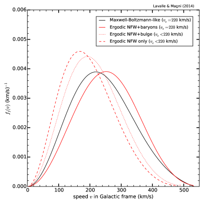
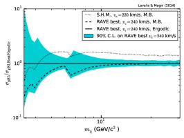
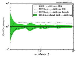
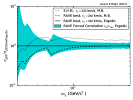
In Fig. 2, we show the differences between the one-dimensional truncated MB speed distribution and the ergodic function, in the MW rest frame. For the latter we explicitly plot the impact of the baryonic components of the gravitational potential (neglecting a component leads to lowering $v_{c}$ and $v_{\rm esc}$) in the left panel. In this panel, we took the P14 best-fit point $\mbox{$v_{\rm esc}$}=533$ km/s associated with the prior $v_{c}=220$ km/s — see Table 2. As expected, the peaks and the mean speeds are different, typically with larger values for the ergodic distribution.

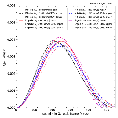
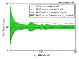
In the right panel of Fig. 2 we compare the MB and ergodic DFs for both P14 best-fit points $\mbox{$v_{\rm esc}$}=533$ and 511 km/s (with priors $v_{c}=220$ and 240 km/s, respectively), showing also the DFs associated with the 90%CL upper and lower corners. What is interesting to note is that while the peaks of the MB DFs move with $v_{c}$, the peaks of the ergodic DFs are almost unaffected; only the high-velocity tails are, which merely reflects the changes in $v_{\rm esc}$.

Figure 3: P14 90% CL results on $v_{\rm esc}$ converted into DD exclusion curves, from the LUX, CRESST-2, and SuperCDMS data. The dashed lines show the SHM exclusion curves (reproducing the original experimental results). Other exclusion curves and bands are obtained using self-consistent ergodic DFs properly correlated to the local DM density inferred from RAVE P14 results (priors) on $v_{\rm esc}$ (on $v_{c}$): plain (dotted) lines correspond to the best-fit values for $v_{\rm esc}$ obtained with the prior $v_{c}=240$ km/s ($v_{c}=220$ km/s) — surrounded by the corresponding 90% CL bands. The dotted-dashed lines represent the P14 $v_{c}$-free case, where the uncertainty bands indicate 1% of the maximum value of the (normalized) likelihood. See the text for more details.

Figure 4: Top panels: experimental limits calculated using the P14 best-fit point with the prior $v_{c}=240$ km/s ($\rho_{\odot}=0.43$ GeV/cm³; $\mbox{$v_{\rm esc}$}=511$ km/s), and associated 90% CL contour. Bottom panels: relative uncertainties with respect to the central value. Left panels: LUX data. Middle panels: SuperCDMS data. Right panels: CRESST-II data. See the text for details.

III.3 RAVE-P14 results on $v_{\rm esc}$ in terms of direct detection limits

Before converting P14 results on $v_{\rm esc}$ in terms of DD limits, we stress again that not only do they affect the whole WIMP velocity DF ($v_{c}$, $v_{\rm esc}$, and the velocity dispersion), but also the local DM density, as already shown in Sec. II.3. We first recall the effects of the main parameters on the DD exclusion curves:

• $\mbox{$v_{\rm esc}$}+v_{c}+V_{\odot}$: defines the average WIMP mass threshold $m_{\chi}^{\rm min}$ given an atomic target and a recoil energy threshold, by solving $v_{\rm min}(E_{\rm th},\mbox{$m_{\chi}$},M)=\mbox{$v_{\rm esc}$}+v_{c}+V_{\odot}$ — see Eq. (19). This corresponds to the position on the mass axis of the asymptote $\sigma_{\rm max}\to\infty$ of the upper limit on the SI cross section (the larger $v_{\rm esc}$ and/or $v_{c}$ the lower the mass threshold).

• $v_{c}$: impact on the relative position of the maximum sensitivity of a DD experiment (for a given atomic target); a larger $v_{c}$ globally shifts the cross section limit curve to the left while not fully affecting the asymptote at the mass threshold, for which $v_{\rm esc}$ is also relevant.

• Velocity dispersion: the larger the dispersion, the larger the sensitivity peak (in the SHM, it is fixed by $v_{c}$).

• Local DM density: global linear and vertical shift of the exclusion curve.

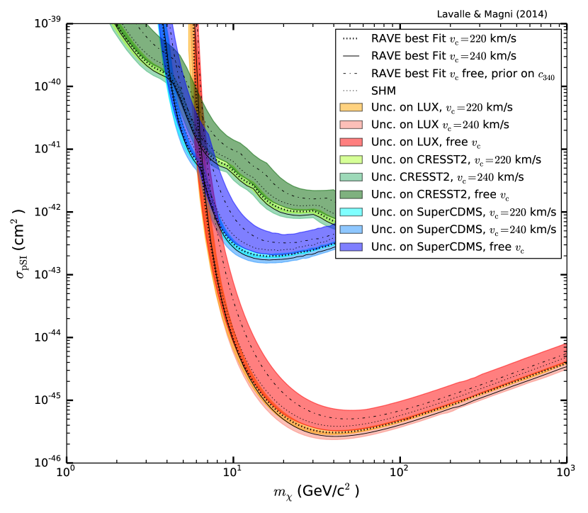
At this stage, we can already notice a few features from P14 results with the help of Fig. 1. First, we see that there is a strong correlation between the circular velocity $v_{c}$ and the local DM density $\rho_{\odot}$, while the latter is poorly correlated with $v_{\rm esc}$. Second, we note that though the two P14 best-fit points with priors on $v_{c}$ exhibit an anticorrelation between $v_{c}$ and $v_{\rm esc}$, this is no longer the case when $v_{c}$ is left free. While this is somewhat contradictory with P14 comments, this implies that the $v_{c}$-free case would provide constraints on $v_{\rm esc}$ independent of $v_{c}$ and $\rho_{\odot}$. Since there are different choices in P14 as for either the priors on $v_{c}$ or the prior on the dark halo concentration, there may be several ways to investigate how the constraints on $v_{\rm esc}$ affect the DD exclusion curves. Here, we first consider the three P14 results independently before comparing them together. For the sake of illustration, we will compute the DD limits by using the LUX results Akerib et al. (2014) as a reference for xenon experiments, the SuperCDMS results Agnese et al. (2014a) as a reference for Germanium experiments, and the CRESST-II results CRESST Collaboration et al. (2014) as a reference for multitarget experiments. As of today, these experiments provide the most stringent combined bounds on the spin-independent cross section for low WIMP masses (assuming elastic scattering and no isospin violation). More technical details are given in the Appendix.

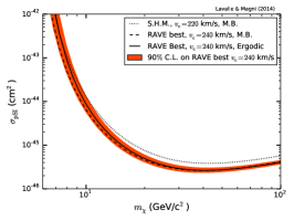
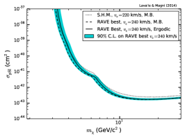
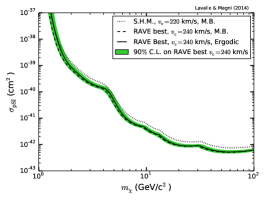
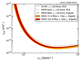
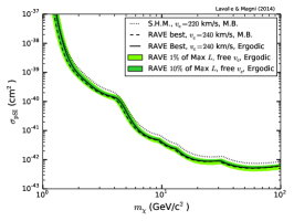
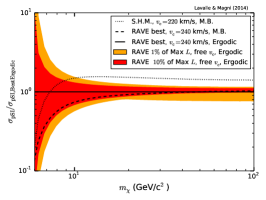
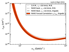
In Fig. 3, we show the exclusion curves obtained in the $\sigma_{p}$-$m_{\chi}$ plane with the uncertainty contours associated with the astrophysical configurations derived from the three P14 best-fit points: (i) the best-fit points with priors $v_{c}=220/240$ km/s and associated 90% CL uncertainty bands and (ii) the best-fit point with free $v_{c}$ (plus an additional prior on the concentration) and associated uncertainty band corresponding to 1% of maximum likelihood in the $M_{340}$-$c_{340}$ plane, rougly matching a 90% CL in the $v_{\rm esc}$-$v_{c}$ plane (see the discussion in Sec. II.3). These curves have been derived by using ergodic DFs that self-consistently correlate the dark halo parameters with $v_{\rm esc}$ and $v_{c}$. We also report on the same plot the exclusion curves calculated from the SHM, with the parameters given in Eq. (26). We may note that the best-fit points associated with priors on $v_{c}$ lead to similar curves and bands, in particular in the low WIMP mass region. This is due to the anticorrelation between $v_{c}$ and $v_{\rm esc}$, which is such that the sum $v_{c}+\mbox{$v_{\rm esc}$}$, relevant to characterize the WIMP mass threshold, remains almost constant. From Fig. 1, we also see that $\rho_{\odot}$ spans only a reduced range of $\sim[0.35,0.47]$ GeV/cm³ for these two points, which leads to less than $\pm 15$% of relative difference in the predicted event rate. In contrast, the exclusion curves associated with the $v_{c}$-free case have (i) a slight offset toward larger WIMP masses while (ii) lying slightly above the others with a larger uncertainty. This is due to (i) the prior on the concentration parameter that forces small values of $v_{c}$ while not affecting $v_{\rm esc}$, and, as a result, to (ii) lower values of $\rho_{\odot}$ spanning the less favorable, while larger range $[0.15,0.35]$ GeV/cm³. We will further comment on the $v_{c}$-free case in Sec. III.4. In comparison, the SHM curves (aimed at reproducing the limits published by the experimental collaborations) lie in between, and are less constraining than the P14 parameters with priors on $v_{c}$.

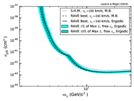
As a reference case to investigate more deeply the uncertainties coming from these P14 results on $v_{\rm esc}$, let us first focus on the best-fit P14 point with the $v_{c}=240$ km/s prior, which we assume to be the most motivated case (see the discussion in Sec. III.4.1). In Fig. 4, we display the exclusion curves and the associated 90% CL uncertainties for this astrophysical configuration (this corresponds to zooming on and decomposing the $v_{c}=$240 km/s case in Fig. 3). The LUX (SuperCDMS, CRESST-II) limits are shown in the left (middle, right) panels; the absolute (relative) uncertainties are given in the top (bottom) panels. We also compare the limits obtained from the ergodic DF to those calculated from the SHM model on the one hand, and from the MB DF with the P14 values for the astrophysical parameters on the other hand. The fact that the P14 escape speed estimate $\mbox{$v_{\rm esc}$}=511^{+48}_{-35}$ (90% CL) converts into $\rho_{\odot}=0.43\pm 0.05$ GeV/cm³ explains why the ergodic limit is more constraining, by $\sim 40$%, than the SHM one ($\rho_{\odot}=0.3$ GeV/cm³) over a large part of the depicted WIMP mass range. In contrast, the SHM limit beats the ergodic one at very low WIMP masses because $v_{\rm esc}$ itself affects the effective WIMP mass threshold: it is set to 544 km/s in the SHM (i.e. $v_{c}+\mbox{$v_{\rm esc}$}=764$ km/s), while the P14 best-fit point (for $v_{c}=240$ km/s) corresponds to $v_{\rm esc}$=511 km/s (i.e. $v_{c}+\mbox{$v_{\rm esc}$}=751$ km/s). Interestingly, we also see the differences induced by different DFs while using the same astrophysical inputs, by comparing the MB and ergodic curves. The former is actually more constraining at energy recoils leading to $v_{\rm min}$ larger than the peak velocity of the DFs. This is because the MB DF exhibits a less steep tail at high velocities than the ergodic DF (see Fig. 2, right panel). This illustrates why not only is the escape speed important in the low WIMP mass region, but also the high-velocity tail of the DF, and thereby the DF itself (see a similar discussion in Ref. Lisanti et al. (2011)). Finally, we may notice that the relative uncertainties in the exclusion curves for this specific P14 point saturate around $\sim\pm 10$% (90% CL) at large WIMP masses, which is mostly set by the allowed range in $\rho_{\odot}$. In the low WIMP mass region, the high-velocity tail and $v_{\rm esc}$ come also into play, and the uncertainties strongly degrade, obviously, as the maximum possible recoil energy approaches the experimental energy threshold. This can clearly be observed in the case of LUX, the efficiency of which drops for WIMP masses below $\sim 8$ GeV (Fig. 4, bottom left panel). However, we may also remark about the nice complementarity between the different experiments that employ different target atoms, as one reaches a relative uncertainty $\sim\pm 30$% for the CRESST-2 proxy down to WIMP masses $\sim 3$ GeV. The bumps appearing in the bottom middle and right panels of Fig. 4 (corresponding to SuperCDMS and CRESST-II) not only come from the differences in the atomic targets, but also from the impact of the observed nuclear-recoil-like events on the maximum gap method Yellin (2002) that we used to derive the exclusion curves (see more details in the Appendix).

At this stage, it is still difficult to draw strong conclusions as for the overall uncertainties in the exclusion curves induced by the P14 results without questioning more carefully the initial assumptions or priors — we will proceed so in Sec. III.4. Nevertheless, we can already emphasize that a self-consistent use of these estimates of $v_{\rm esc}$ is not straightforward (for instance, one cannot just vary $v_{\rm esc}$ in a given CL range irrespective of the other astrophysical parameters). A proper use must take the correlations between all the relevant astrophysical parameters into account. Indeed, we have just seen that not only is the WIMP mass threshold affected (direct consequence of varying $\mbox{$v_{\rm esc}$}+v_{c}$), but also the global event rate, as $\rho_{\odot}$ must be varied accordingly.

III.4 Discussion

In this section, we wish to examine the previous results in light of independent constraints on the astrophysical inputs. As we saw, P14 provided three best-fit configurations each based on different priors. The most conservative approach would be to relax fixed priors as much as possible, as all astrophysical parameters are affected by uncertainties. We will therefore focus on the $v_{c}$-free case in the following.

Figure 5: Top panels: experimental limits calculated with a combination of the P14 $v_{c}$-free analysis with additional constraints on $v_{c}$ from Ref. Reid et al. (2014). Bottom panels: relative uncertainties with respect to the $v_{c}=240$ km/s best-fit point of P14. Left panels: LUX data. Middle panels: SuperCDMS data. Right panels: CRESST-II data. See the text for details.

III.4.1 Additional and independent constraints on $v_{c}$

In Fig. 1, we see that the prior on the concentration model forces the fit to low values of $v_{c}$, with a central value $v_{c}=196$ km/s; the best-fit point and associated uncertainty region lead to the DD exclusion curves flagged “$v_{c}$-free” in Fig. 3. Nevertheless, this prior on concentration is based upon Ref. Macciò et al. (2008), which studies the halo mass-concentration relation in cosmological simulations that do not contain baryons. Since we now know that baryons may affect the structuring of dark matter significantly on galactic scales (see e.g. Refs.  Guedes et al. (2011); Pontzen (2014); Mollitor et al. (2014)), the motivation to use such a constraint appears to us to be rather weak. In the following, we will therefore relax this prior and rather consider the entire range provided by the P14 likelihood in the $v_{c}$-$v_{\rm esc}$ plane.

If we relax the prior on the concentration law, we see that although the astrophysical parameters relevant to DD are not much correlated with $v_{\rm esc}$ (see the explanation and warning in Sec. II.3), which lies in the range $\sim 500$-570 km/s, the local DM density $\rho_{\odot}$ is strongly correlated with the circular velocity $v_{c}$, which was explored over a large range of $\sim 160$-260 km/s. We recall that in their $v_{c}$-free analysis, P14 originally explored the $M_{340}$-$c_{340}$ plane that we had to convert back into $v_{c}$-$v_{\rm esc}$ for the sake of DD interpretations.

The circular velocity $v_{c}$ can actually be constrained independently of any assumption on the dark halo modeling. Indeed, for instance, one can use measures of trigonometric parallaxes and proper motions of stars to reconstruct the local kinematics, where the only model ingredients to consider are the circular and peculiar motions of the Sun in the Milky Way rest frame, and the distance of the Sun to the Galactic center. It turns out that the ratio $v_{c}/\mbox{$r_{\odot}$}$ is often better constrained than $v_{c}$ and $r_{\odot}$ individually. More precisely, in the absence of a prior on the peculiar velocity of the Sun, these observations constrain the ratio $(v_{c}+V_{\odot})/\mbox{$r_{\odot}$}$ (see for instance Refs. Reid et al. (2009); McMillan (2011); Reid et al. (2014)). Since both $r_{\odot}$ and the peculiar velocity of the Sun have been fixed in P14, we could still use these independent constraints on $v_{c}/\mbox{$r_{\odot}$}$ to delineate an observationally motivated range for $v_{c}$. Fortunately, the recent study in Ref. Reid et al. (2014) on local kinematics, based on a large statistics of parallaxes and proper motions of masers associated with young and massive stars, provides results that can be used rather straightforwardly as some of their priors are similar to those of P14. This avoids relying on the $(v_{c}+V_{\odot})/\mbox{$r_{\odot}$}$ ratio, which induces the risk of underestimating the errors for fixed values of $V_{\odot}$ and $r_{\odot}$. Indeed, in their Bayesian fit model B1 (associated with the cleanest data sample), the authors of Ref. Reid et al. (2014) take as a prior on the peculiar velocity the results of Ref. Schönrich et al. (2010), also chosen by P14 [see Eq. (2)]. They then derive a best-fit value for $\mbox{$r_{\odot}$}=8.33\pm 0.16$ kpc, fully consistent with the 8.28 kpc adopted in P14. Accordingly, they get the range for $v_{c}$,

$$v_{c}=243\pm 6\;{\rm km/s}\,(1\,\sigma),$$ (34)

that we can use directly (we will actually use the 2-$\sigma$ range $\pm 12$ km/s for a more realistic discussion on the uncertainties — the posterior PDF is found close to Gaussian Reid et al. (2014)). We report this range as a green band in Fig. 1, which represents an independent constraint in the $v_{c}$-$v_{\rm esc}$ plane. We emphasize that this additional constraint does not depend on the dark halo model, as it was extracted from parallax and proper motion reconstruction methods. We only need to make sure that our Galactic mass models are consistent with a last feature of model B1 of Ref. Reid et al. (2014) regarding the local derivative of the circular velocity, $dv_{c}/dR=-0.2\pm 0.4$ km/s/kpc, pointing to an almost flat local rotation curve. We have checked that this is the case almost everywhere in the relevant part of the uncertainty band of Fig. 1 within three standard deviations. The largest tensions with respect to the range allowed for $dv_{c}/dR$ arise for the lowest values allowed for $v_{\rm esc}$, which force the scale radius $r_{s}$ of the NFW profile to be smaller than $r_{\odot}$ and thereby affect the local slope of the rotation curve. This is not favored by independent analyses (see e.g. Ref. McMillan (2011)), and interestingly enough, this disfavored zone also corresponds to the lowest values of the local DM density.

In Fig. 1, we have reported this 2-$\sigma$ range for $v_{c}$. It crosses the full blue band of the $v_{c}$-free case of P14, which allows to define a constrained region in the plane $v_{c}$-$v_{\rm esc}$, that we will use to determine the uncertainties implied for DD exclusion curves. We recall that the blue band corresponds to likelihood values larger than 1% of the maximum in the plane $M_{340}$-$c_{340}$, which we may interpret as $\sim 2$-$\sigma$ uncertainties in the plane $v_{\rm esc}$-$v_{c}$ relevant to DD calculations (see the discussion in Sec. II.3). We note that this region allows for large values of the local DM density, up to 0.55 GeV/cm³. This is actually consistent with the tendency found in recent independent studies (see e.g. Refs. Bovy et al. (2012); Bienaymé et al. (2014); Piffl et al. (2014b)), and reinforces the potential of DD experiments. However, we warn the reader that the dynamical mass model used in the present study is rather simplistic and is not meant to discuss the local amount of DM. In particular, all the baryonic matter – including gas and dust in addition to stars – is bound to the stellar disk and bulge components of the model, while additional components may have different spatial properties (see e.g. Ref. Catena and Ullio (2010)). This mass model is actually imposed by consistency in properly using P14 results, which were obtained under the assumption of this specific mass model. We may still note that the parameters of this model are in reasonable agreement with the recent study of Ref. Kafle et al. (2014), based on a dedicated global kinematic analysis.

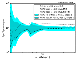
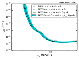
In Fig. 5 we show the uncertainties obtained when considering the combination of the P14 $v_{c}$-free case with the additional constraints on $v_{c}$ discussed above. These plots are similar to those of Fig. 4 as only the uncertainty contours change. In particular, we have also reported the exclusion curves obtained with the P14 “$v_{c}$=240 km/s” best-fit configuration, which are shown to lie within the contours of the $v_{c}$-free case (plus independent and additional constraints on $v_{c}$). This can easily be understood from Fig. 1. The changes in the uncertainty contours can again be understood in terms of local DM density, which is found in the range [0.37,0.57] GeV/cm³. This sets the relative uncertainties to $\sim\pm 20$% for large WIMP masses, while they further degrade toward low WIMP masses because of the additional effects from $v_{\rm esc}$ and $v_{c}$.

Figure 6: Same as Fig. 5, but for the $v_{c}$-$v_{\rm esc}$ range supposed to properly take the anticorrelation into account (cite dotted lines in Fig. 1).

Figure 7: Effect of not considering the correlation of the astrophysical parameters (local DM density and relevant speeds) in drawing the relative uncertainty in the LUX DD exclusion curve. The dashed region is the same as the colored region in the bottom left panel of Fig. 6.

III.4.2 Speculating beyond P14

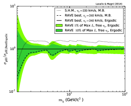
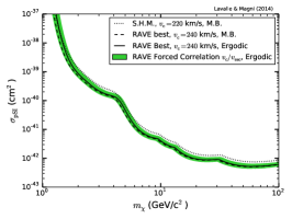
Because of the caveats affecting the $v_{c}$-free case of P14 (see the discussion in Sec. II.3), and in order to try to recover a better consistency in the Galactic mass modeling, we may try to further speculate about what a self-consistent $v_{c}$-free band would look like. The P14 argument that $v_{c}$ and $v_{\rm esc}$ should linearly anticorrelate is sound as it is based on a purely geometrical reasoning (the fact that the stellar sample is completely biased toward negative longitudes). Therefore, it is quite reasonable to think that the dotted lines in Fig. 1, that relate the two best-fit points and errors associated with the 220 and 240 km/s priors on $v_{c}$, may represent a more consistent range than the $v_{c}$-free band. As before, we also investigate how the uncertainties export to DD, using again the additional 2-$\sigma$ constraints on $v_{c}$ from Ref. Reid et al. (2014) — see Eq. (34).

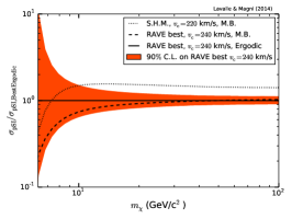
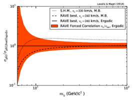
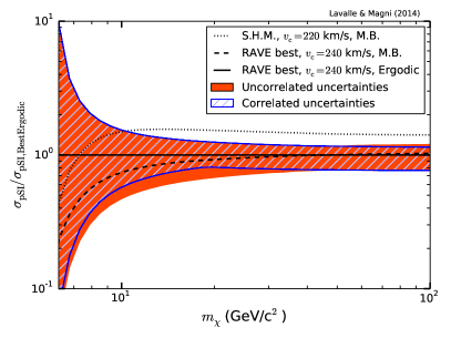
We show our results in Fig. 6, similar to those of Fig. 5, though likely more consistent with the original data used in P14 (because of the supposed anticorrelation between $v_{\rm esc}$ and $v_{c}$). As expected, the relative uncertainties improve on the entire WIMP mass range. They improve down to $\sim\pm 10$% in the large WIMP mass region. While not spectacular, this still illustrates the need to account for as many astrophysical correlations as possible in deriving the DD limits. To quantify this, we show the difference in the relative uncertainty band between the correlated and uncorrelated cases in Fig. 7, using the LUX setup — where the dashed region shows the correlated uncertainty band obtained in the bottom left panel of Fig. 6. The improvement is not as tremendous as one would naively expect, but still clearly visible around the maximum sensitivity region: this is due to the fact that large speeds ($v_{c}$ and $v_{\rm esc}$) are dynamically correlated with a large local DM density, which tends to maximize the uncertainty in the low WIMP mass region (there is still a gain in the intermediate region). Nevertheless, we stress that accounting for these dynamical correlations would become critical when using DD to check a WIMP model that would be invoked to interpret any putative indirect detection signal (the WIMP annihilation rate scales like $\rho^{2}_{\odot}$).

IV Conclusion

In this article, we have studied the impact of the recent estimate of the Galactic escape speed $v_{\rm esc}$ from Ref. Piffl et al. (2014a) (P14) in deriving the DD exclusion curves. We note that this observable is difficult to reconstruct, and the method used in P14, as recognized by the authors, is potentially subject to systematic errors. Nevertheless, these constraints are independent of those coming from studies of rotation curves, and thereby may provide complementary information on the WIMP phase space. We have shown that the conversion of these results is highly nontrivial, as the constraints on $v_{\rm esc}$ are obtained from a series of assumptions that relate each value of $v_{\rm esc}$ to a different set of parameters for the dark halo profile. This implies that one cannot use the different $v_{\rm esc}$ ranges provided by P14 blindly and irrespective of these assumptions (as is often done by implementing them with flat or Gaussian priors in likelihood or Monte Carlo Markov chain calculations). We have assumed spherical symmetry and gone beyond the Maxwell-Boltzmann approximation by considering ergodic WIMP velocity DFs. This method ensures a self-consistent physical connection between the DFs and the underlying Galactic mass model. In particular, all local variables relevant to DD calculations, i.e. the average WIMP speed, the dispersion velocity, and the local DM density, are consistently dynamically correlated in this approach.

We have studied the three best-fit configurations provided by P14, two with priors on the circular velocity $v_{c}$ (220 and 240 km/s), and one with $v_{c}$ left free. These configurations are shown in the $v_{c}$-$v_{\rm esc}$ plane in Fig. 1. As the first two appeared to us too specific, we concentrated on the latest, which was originally optimized for Milky Way mass estimates (we had to convert the P14 results from the $c_{340}$-$M_{340}$ plane to the $v_{c}$-$v_{\rm esc}$ plane). We discovered that the anticorrelation between $v_{c}$ and $v_{\rm esc}$ arising from the biased locations of the stars of the RAVE-P14 sample toward negative longitudes, and found in the $v_{c}=220$-240 km/s cases, was no longer present. This is actually due to the use of the posterior PDF for $v_{\rm esc}$ with the $v_{c}=220$ km/s prior as a proxy, which could hardly be divined from Fig. 13 in P14. We therefore further speculated on what a fully self-consistent $v_{c}$-free case could look like, and considered this guess as an alternative. Finally, we accounted for independent constraints on $v_{c}$ from Ref. Reid et al. (2014), which have the advantage of being almost fully independent of the Galactic mass model. This has driven us to favor large $v_{c}$ regions, around 240 km/s, which are in principle associated with lower escape speeds in P14.

We have translated these P14 results in terms of DD exclusion curves focusing on the LUX, SuperCDMS, and CRESST-II experiments as references. We emphasize that a self-consistent use of these P14 results implies rather large values of the local DM density and thereby more constraining exclusion curves (up to $\sim$40% more). Interestingly enough, this is consistent with several independent recent results on the local DM density (see e.g. Refs. Bovy et al. (2012); Bienaymé et al. (2014); Piffl et al. (2014b)). This is good news for direct DM searches as this tends to increase their potential of discovery or exclusion. We have also investigated the associated relative uncertainties, and shown that they are highly nontrivial as P14 values of $v_{\rm esc}$ are correlated with other astrophysical parameters, as already stated above. We have shown that taking P14 results at face value (plus eventually additional independent constraints on $v_{c}$) converts into moderate uncertainties, down to $\sim\pm 10$% in the regime where the experiments can trigger on the whole phase space (large WIMP masses). This is not to be considered as a definitive estimate of the overall astrophysical uncertainties, as both P14 and our phase-space modeling suffer from simplifying assumptions (simplistic baryonic mass model, spherical symmetry, etc.); this is still indicative, and compares to the low-edge estimates of other studies based on rotation curves (see e.g. Ref. Fairbairn et al. (2013)). When getting closer to the high-velocity tail (low WIMP masses), the uncertainties explode as the experimental efficiency drops, but we have illustrated the nice complementarity between the experiments using different target atoms in this regime. This complementarity allows to maintain a moderate uncertainty of $\sim\pm 20$% down to WIMP masses of a few GeV. Nevertheless, since the SHM value for the sum $v_{c}+\mbox{$v_{\rm esc}$}$ is 764 km/s (based on S07), i.e. slightly more than the 751 km/s found from the more recent P14 estimate (with the prior $v_{c}=240$ km/s), the generic outcome is that we find an effective WIMP mass threshold slightly heavier than in the SHM.

There are several limitations in our analysis. First, the Galactic mass model is rather simple and the baryonic content has been fixed in P14. Unfortunately, we cannot go beyond this choice as this would no longer be consistent with P14 results. Second, we made the assumption that the WIMP phase-space was governed by energy in a spherically symmetric system, which led to the derivation of ergodic velocity DFs. While this approach self-consistently correlates the local velocity features and the local DM density to the full gravitational potential, it remains to be investigated in detail whether it reliably captures the dynamics at stake in spiral galaxies. Some works do indicate that this approach provides a reasonable description of cosmological simulation results (see e.g. Refs. Wojtak et al. (2008); Lisanti et al. (2011)), but it is obvious that more studies will be necessary to clarify this issue. We plan to discuss this in more detail in a forthcoming paper. Still, it is less ad hoc an assumption than using the Maxwell-Boltzmann velocity distribution.

Finally, we stress that our study is complementary to those based e.g. on rotation curves, as it relies on different, and independent, observational constraints. Further merging these different sets of constraints would be interesting in the future. Moreover, because of these dynamical correlations inherently arising in the local astrophysical parameters, which was continuously underlined throughout this paper, several improvements could also be expected in the complementary use of direct and indirect detection constraints in order to exclude or validate some WIMP scenarios.

Appendix A Direct detection data and limits

For every experiment, we briefly summarize the most important quantities that allow us to reproduce the experiment results.

A.1 LUX

LUX is a liquid xenon time-projection chamber experiment which currently runs with a 370 kg target. We use the results released by the collaboration in Ref. Akerib et al. (2014). The first run described there collected $85.3$ days of data, with a detector fiducial xenon mass of 118 kg. The next 300-day run expected for the end of 2014 should improve the sensitivity by a factor of 5.

As the published results are based on a private likelihood analysis, we cannot reproduce them exactly. Instead, we follow the approach detailed in Ref. Del Nobile et al. (2014), relying on the maximum gap method (MGM) Yellin (2002) over an S1 range of 2-30 photoelectrons, the same as the one used in the private likelihood. In this range, 160 events are observed, all consistent with the predicted background of electronic recoils. Of these events, 24 fall into the calibration nuclear recoil band. Nevertheless, as these events are distributed only in the lower half of the band, while WIMP events should spread over the full range, it is unlikely that a significant part of them really comes from WIMP scatterings. In Ref. Del Nobile et al. (2014), several configurations of event counting are considered to feed the MGM procedure: 0, 1, 3, 5 or all the 24 events. The best matching with the experimental result is obtained for the MGM method run with between 0 and 1 event. As the former better reproduces the experimental curve at low WIMP masses, we adopt this one.

For the experimental efficiency after cuts, we have used Fig. 9 of Ref. Akerib et al. (2014). As in Ref. Del Nobile et al. (2014), we set the counting efficiency to $0$ below $3$ keVnr. We use a Gaussian energy resolution, with a dispersion $\sigma(E_{\rm nr})=\sigma_{\rm PMT}\,Q(E_{\rm nr})$, with $Q(E_{\rm nr})=\frac{4.131}{E_{nr}/KeV}+0.690$ and an S1 single photoelectron resolution of $\sigma_{\rm PMT}=0.37$ photoelectrons.

An indicative conversion from S1 and S2 signals to $E_{\rm nr}$ can be inferred from the contour lines in Fig. 4 of Ref. Akerib et al. (2014). We have used the relation

$$E_{\rm nr}=\frac{{\rm S}1}{L_{y}\,{\cal L}_{\rm eff}}\frac{S_{\rm e}}{S_{\rm n}}$$ (35)

with the light yeld $L_{y}=3$ photoelectrons/keVee and the scintillation quenching $S_{\rm e}=0.54$ for electron recoils and $S_{\rm n}=0.93$ for nuclear recoils from Ref. Sorensen et al. (2009). Even if the value of the Lindhard factor ${\cal L}_{\rm eff}$ in liquid xenon is still subject to debate, we simply assumed the value ${\cal L}_{eff}=0.14$ in this analysis which is not aimed at investigating the compatibility of exclusions with putative signal regions. Finally, we use the Helm form factor Lewin and Smith (1996) to model effects of the nuclear shape on the elastic scattering.

A.2 CRESST-II

The CRESST experiment is a multitarget detector made of CaWO₄ crystals — calcium (Ca), oxygen (O) and Tungsten (W). We base our limits on the recent results released in Ref. CRESST Collaboration et al. (2014), relying on an exposure (before cuts) of 29.35 kg$\cdot$day. The energy range used in the data analysis is $[0.6,40]$ keV, for which we consider all the events collected, i.e. around 77 events. The energies of these events can be inferred from Fig. 1 and from the inset of Fig. 2 of Ref. CRESST Collaboration et al. (2014). We obtain the $90\%$ CL upper limits by means of the MGM, while the original analysis employs the optimum interval method. We use the following atomic target fractions: $f_{\rm Ca}=1/6$, $f_{\rm O}=4/6$, and $f_{\rm W}=1/6$. We accounted for a Gaussian energy resolution with $\sigma=0.107$ keV, and took the experimental efficiency after cuts from the blue curve in Fig. 3 of Ref. CRESST Collaboration et al. (2014).

A.3 SuperCDMS

SuperCDMS is a detector using Ge crystals. A recent data analysis focused on low-mass WIMPs has been released in Ref. Agnese et al. (2014a), based on an exposure of 577 kg$\cdot$day. The energy range used in the data analysis is $[1.6,10]$ keV_nr, in which 11 candidate events were observed for a background expectation of 6.198 events. Their energies are listed in Table I of Ref. Agnese et al. (2014a). While the experiment limit is derived from the optimum interval method without background subtraction Yellin (2002), we still use the MGM which gives similar results. We take into account the experimental efficiency that we obtain from the red curve of Fig. 1 in Ref. Agnese et al. (2014a), and which is an exposure-weighted sum of the measured efficiency for each detector and period. We assumed a Gaussian energy resolution, and for lack of better information we used the same energy dispersion as in CDMSLite Agnese et al. (2014b), $\sigma=14$ eV_ee (which corresponds to 87.5 eV_nr after conversion by means of the Lindard theory, as done in Ref. Agnese et al. (2014b)).

References

- Goodman and Witten (1985) M. W. Goodman and E. Witten, Phys. Rev. D 31, 3059 (1985).
- Drukier et al. (1986) A. K. Drukier, K. Freese, and D. N. Spergel, Phys. Rev. D 33, 3495 (1986).
- Angle et al. (2008) J. Angle et al., Phys. Rev. Lett. 100, 021303 (2008), arXiv:0706.0039 .
- Ahmed et al. (2009) Z. Ahmed et al., Phys. Rev. Lett. 102, 011301 (2009), arXiv:0802.3530 .
- CDMS II Collaboration et al. (2010) CDMS II Collaboration, Z. Ahmed et al., Science 327, 1619 (2010), arXiv:0912.3592 [astro-ph.CO] .
- Armengaud et al. (2011) EDELWEISS Collaboration, E. Armengaud et al., Phys. Lett. B 702, 329 (2011).
- Agnese et al. (2013) R. Agnese et al., Phys. Rev. D 88, 031104 (2013), arXiv:1304.3706 [astro-ph.CO] .
- Aprile et al. (2013) E. Aprile et al., Phys. Rev. D 88, 012006 (2013), arXiv:1304.1427 [astro-ph.IM] .
- Akerib et al. (2014) LUX Collaboration, D. S. Akerib et al., Phys. Rev. Lett. 112, 091303 (2014).
- Primack et al. (1988) J. R. Primack, D. Seckel, and B. Sadoulet, Annu. Rev. Nucl. Part. Sci. 38, 751 (1988).
- Jungman et al. (1996) G. Jungman, M. Kamionkowski, and K. Griest, Phys. Rept. 267, 195 (1996), hep-ph/9506380 .
- Bergström (2000) L. Bergström, Rep. Prog. Phys. 63, 793 (2000), hep-ph/0002126 .
- Bergström (2009) L. Bergström, New J. Phys. 11, 105006 (2009), arXiv:0903.4849 [hep-ph] .
- Bernabei et al. (2000) R. Bernabei et al., Eur. Phys. J. C 18, 283 (2000).
- Bernabei et al. (2013) R. Bernabei et al., Eur. Phys. J. C 73, 2648 (2013), arXiv:1308.5109 [astro-ph.GA] .
- Freese et al. (1988) K. Freese, J. Frieman, and A. Gould, Phys. Rev. D 37, 3388 (1988).
- Aalseth et al. (2011) C. E. Aalseth et al., Phys. Rev. Lett. 106, 131301 (2011), arXiv:1002.4703 [astro-ph.CO] .
- Angloher et al. (2012) G. Angloher et al., Eur. Phys. J. C 72, 1971 (2012), arXiv:1109.0702 [astro-ph.CO] .
- Aalseth et al. (2013) C. E. Aalseth et al., Phys. Rev. D 88, 012002 (2013), arXiv:1208.5737 [astro-ph.CO] .
- Agnese et al. (2014a) SuperCDMS Collaboration, R. Agnese et al., Phys. Rev. Lett. 112, 041302 (2014a), arXiv:1309.3259 [physics.ins-det] .
- CRESST Collaboration et al. (2014) CRESST Collaboration, G. Angloher et al., ArXiv e-prints (2014), arXiv:1407.3146 .
- Lavalle (2010) J. Lavalle, Phys. Rev. D 82, 081302 (2010), arXiv:1007.5253 [astro-ph.HE] .
- Cerdeno et al. (2012) D. G. Cerdeno, T. Delahaye, and J. Lavalle, Nucl. Phys. B 854, 738 (2012), arXiv:1108.1128 [hep-ph] .
- Pradler and Yavin (2013) J. Pradler and I. Yavin, Phys. Lett. B 723, 168 (2013), arXiv:1210.7548 [hep-ph] .
- Pradler et al. (2013) J. Pradler, B. Singh, and I. Yavin, Phys. Lett. B 720, 399 (2013), arXiv:1210.5501 [hep-ph] .
- Davis (2014) J. H. Davis, ArXiv e-prints (2014), arXiv:1407.1052 [hep-ph] .
- Bœhm and Fayet (2004) C. Bœhm and P. Fayet, Nucl. Phys. B 683, 219 (2004), hep-ph/0305261 .
- Kappl et al. (2011) R. Kappl, M. Ratz, and M. W. Winkler, Phys. Lett. B 695, 169 (2011), arXiv:1010.0553 [hep-ph] .
- Ellwanger and Hugonie (2014) U. Ellwanger and C. Hugonie, ArXiv e-prints (2014), arXiv:1405.6647 [hep-ph] .
- Kerr and Lynden-Bell (1986) F. J. Kerr and D. Lynden-Bell, MNRAS 221, 1023 (1986).
- Catena and Ullio (2010) R. Catena and P. Ullio, JCAP 8, 004 (2010), arXiv:0907.0018 [astro-ph.CO] .
- McMillan (2011) P. J. McMillan, MNRAS 414, 2446 (2011), arXiv:1102.4340 [astro-ph.GA] .
- Leonard and Tremaine (1990) P. J. T. Leonard and S. Tremaine, Astrophys. J. 353, 486 (1990).
- Steinmetz et al. (2006) M. Steinmetz et al., Astron. J. 132, 1645 (2006), astro-ph/0606211 .
- Smith et al. (2007) M. C. Smith et al., MNRAS 379, 755 (2007), astro-ph/0611671 .
- McCabe (2010) C. McCabe, Phys. Rev. D 82, 023530 (2010), arXiv:1005.0579 [hep-ph] .
- Piffl et al. (2014a) T. Piffl et al., Astron. Astroph. 562, A91 (2014a), arXiv:1309.4293 [astro-ph.GA] .
- Kafle et al. (2014) P. R. Kafle, S. Sharma, G. F. Lewis, and J. Bland-Hawthorn, Astrophys. J. 794, 59 (2014), arXiv:1408.1787 .
- Green (2010) A. M. Green, JCAP 10, 034 (2010), arXiv:1009.0916 [astro-ph.CO] .
- Green (2012) A. M. Green, Mod. Phys. Lett. A 27, 1230004 (2012), arXiv:1112.0524 [astro-ph.CO] .
- Freese et al. (2013) K. Freese, M. Lisanti, and C. Savage, Rev. Mod. Phys. 85, 1561 (2013).
- Arina et al. (2011) C. Arina, J. Hamann, and Y. Y. Y. Wong, JCAP 9, 022 (2011), arXiv:1105.5121 [hep-ph] .
- Catena and Ullio (2012) R. Catena and P. Ullio, JCAP 5, 005 (2012), arXiv:1111.3556 [astro-ph.CO] .
- Fairbairn et al. (2013) M. Fairbairn, T. Douce, and J. Swift, Astropart. Phys. 47, 45 (2013), arXiv:1206.2693 [astro-ph.CO] .
- Bozorgnia et al. (2013) N. Bozorgnia, R. Catena, and T. Schwetz, JCAP 12, 050 (2013), arXiv:1310.0468 [astro-ph.CO] .
- Beers et al. (2000) T. C. Beers et al., Astron. J. 119, 2866 (2000), astro-ph/0003103 .
- Binney and Tremaine (2008) J. Binney and S. Tremaine, Galactic Dynamics: Second Edition. ISBN 978-0-691-13026-2 (HB). (Princeton University Press, NJ USA, 2008).
- Scannapieco et al. (2009) C. Scannapieco, S. D. M. White, V. Springel, and P. B. Tissera, MNRAS 396, 696 (2009), arXiv:0812.0976 .
- Gillessen et al. (2009) S. Gillessen et al., Astrophys. J. 692, 1075 (2009), arXiv:0810.4674 .
- Schönrich et al. (2010) R. Schönrich, J. Binney, and W. Dehnen, MNRAS 403, 1829 (2010), arXiv:0912.3693 [astro-ph.GA] .
- Hernquist (1990) L. Hernquist, Astrophys. J. 356, 359 (1990).
- Miyamoto and Nagai (1975) M. Miyamoto and R. Nagai, Pub. Astron. Soc. Jap. 27, 533 (1975).
- Navarro et al. (1997) J. F. Navarro, C. S. Frenk, and S. D. M. White, Astrophys. J. 490, 493 (1997), astro-ph/9611107 .
- Schönrich (2012) R. Schönrich, MNRAS 427, 274 (2012), arXiv:1207.3079 [astro-ph.GA] .
- Reid et al. (2014) M. J. Reid et al., Astrophys. J. 783, 130 (2014), arXiv:1401.5377 [astro-ph.GA] .
- Macciò et al. (2008) A. V. Macciò, A. A. Dutton, and F. C. van den Bosch, MNRAS 391, 1940 (2008), arXiv:0805.1926 .
- Stanek and Garnavich (1998) K. Z. Stanek and P. M. Garnavich, Astrophys. J. Lett. 503, L131 (1998), astro-ph/9802121 .
- Riess et al. (2012) A. G. Riess, J. Fliri, and D. Valls-Gabaud, Astrophys. J. 745, 156 (2012), arXiv:1110.3769 [astro-ph.CO] .
- Lewin and Smith (1996) J. D. Lewin and P. F. Smith, Astropart. Phys. 6, 87 (1996).
- Green (2003) A. M. Green, Phys. Rev. D 68, 023004 (2003), astro-ph/0304446 .
- Lee et al. (2013) S. K. Lee, M. Lisanti, and B. R. Safdi, JCAP 11, 033 (2013), arXiv:1307.5323 [hep-ph] .
- McCabe (2014) C. McCabe, JCAP 2, 027 (2014), arXiv:1312.1355 [astro-ph.CO] .
- Eddington (1916) A. S. Eddington, MNRAS 76, 525 (1916).
- Ullio et al. (2001) P. Ullio, H. Zhao, and M. Kamionkowski, Phys. Rev. D 64, 043504 (2001), astro-ph/0101481 .
- Vergados and Owen (2003) J. D. Vergados and D. Owen, Astrophys. J. 589, 17 (2003), astro-ph/0203293 .
- Fornasa and Green (2014) M. Fornasa and A. M. Green, Phys. Rev. D 89, 063531 (2014), arXiv:1311.5477 .
- Wojtak et al. (2008) R. Wojtak et al., MNRAS 388, 815 (2008), arXiv:0802.0429 .
- Lisanti et al. (2011) M. Lisanti, L. E. Strigari, J. G. Wacker, and R. H. Wechsler, Phys. Rev. D 83, 023519 (2011), arXiv:1010.4300 [astro-ph.CO] .
- Yellin (2002) S. Yellin, Phys. Rev. D 66, 032005 (2002), physics/0203002 .
- Guedes et al. (2011) J. Guedes, S. Callegari, P. Madau, and L. Mayer, Astrophys. J. 742, 76 (2011), arXiv:1103.6030 [astro-ph.CO] .
- Pontzen (2014) A. Pontzen, Phys. Rev. D 89, 083010 (2014), arXiv:1402.0506 .
- Mollitor et al. (2014) P. Mollitor, E. Nezri, and R. Teyssier, ArXiv e-prints (2014), arXiv:1405.4318 .
- Reid et al. (2009) M. J. Reid et al., Astrophys. J. 700, 137 (2009), arXiv:0902.3913 [astro-ph.GA] .
- Bovy et al. (2012) J. Bovy et al., Astrophys. J. 759, 131 (2012), arXiv:1209.0759 [astro-ph.GA] .
- Bienaymé et al. (2014) O. Bienaymé et al., ArXiv e-prints (2014), arXiv:1406.6896 .
- Piffl et al. (2014b) T. Piffl et al., ArXiv e-prints (2014b), arXiv:1406.4130 .
- JabRef Development Team (2014) JabRef Development Team, JabRef (2014).
- Del Nobile et al. (2014) E. Del Nobile, G. B. Gelmini, P. Gondolo, and J.-H. Huh, JCAP 3, 014 (2014), arXiv:1311.4247 [hep-ph] .
- Sorensen et al. (2009) P. Sorensen et al., Nucl. Instrum. Methods Phys. Res. A 601, 339 (2009).
- Agnese et al. (2014b) SuperCDMS Collaboration, R. Agnese et al., Phys. Rev. Lett. 112, 241302 (2014b), arXiv:1402.7137 [hep-ex] .