Maëlle Salmon, Dirk Schumacher, Michael Höhle surveillance: Aberration detection in R Public health surveillance aims at lessening disease burden, e.g., in case of infectious diseases by timely recognizing emerging outbreaks. Seen from a statistical perspective, this implies the use of appropriate methods for monitoring time series of aggregated case reports. This paper presents the tools for such automatic aberration detection offered by the R package surveillance. We introduce the functionality for the visualization, modelling and monitoring of surveillance time series. With respect to modelling we focus on univariate time series modelling based on generalized linear models (GLMs), multivariate GLMs, generalized additive models and generalized additive models for location, shape and scale. This ranges from illustrating implementational improvements and extensions of the well-known Farrington algorithm, e.g., by spline-modelling or by treating it in a Bayesian context. Furthermore, we look at categorical time series and address overdispersion using beta-binomial or Dirichlet-Multinomial modelling. With respect to monitoring we consider detectors based on either a Shewhart-like single timepoint comparison between the observed count and the predictive distribution or by likelihood-ratio based cumulative sum methods. Finally, we illustrate how surveillance can support aberration detection in practice by integrating it into the monitoring workflow of a public health institution. Altogether, the present article shows how well surveillance can support automatic aberration detection in a public health surveillance context. R, surveillance, outbreak detection, statistical process control R, surveillance, outbreak detection, statistical process control Maëlle Salmon
Department for Infectious Diseases Epidemiology
Robert Koch Institut Berlin
Seestrasse 10
13353 Berlin, Germany
E-mail:
URL: http://www.normalesup.org/~masalmon/

Dirk Schumacher
Department for Infectious Diseases Epidemiology
Robert Koch Institut Berlin
Seestrasse 10
13353 Berlin, Germany
E-mail:
URL: http://www.dirk-schumacher.net/

Michael Höhle
Department of Mathematics
Stockholm University
Kräftriket
106 91 Stockholm,Sweden E-mail:
URL: http://www.math.su.se/~hoehle/

Monitoring Count Time Series in R: Aberration Detection in Public Health Surveillance

Introduction

Nowadays, the fight against infectious diseases does not only require treating patients and setting up measures for prevention but also demands the timely recognition of emerging outbreaks in order to avoid their expansion. Along these lines, health institutions such as hospitals and public health authorities collect and store information about health events – typically represented as individual case reports containing clinical information, and subject to specific case definitions. Analysing these data is crucial. It enables situational awareness in general and in particular the timely detection of aberrant counts empowering the prevention of additional disease cases through early interventions. For any specific aggregation of characteristics of events, such as over-the-counter sales of pain medication, new cases of foot-and-mouth disease among cattle, or adults becoming sick with hepatitis C in Germany, data can be represented as time series of counts with days, weeks, months or years as time units of the aggregation. Abnormally high or low values at a given time point can reveal critical issues such as an outbreak of the disease or a malfunction of data transmission. Thus, identifying aberrations in the collected data is decisive, for human as well as for animal health.

In this paper we present the R package surveillance, which implements a range of methods for aberration detection in time series of counts and proportions. Statistical algorithms provide an objective and reproducible analysis of the data and allow the automation of time-consuming aspects of the monitoring process. In the recent years, a variety of such tools has flourished in the literature. Reviews of methods for aberration detection in time series of counts can be found in Buckeridge et al. (2005) and Unkel et al. (2012). However, the great variety of statistical algorithms for aberration detection can be a hurdle to practitioners wishing to find a suitable method for their data. It is our experience that ready-to-use and understandable implementation and the possibility to use the methods in a routine and automatic fashion are the criteria most important to the epidemiologists.

The package offers an open-source implementation of state-of-the-art methods for the prospective detection of outbreaks in count data time series with established methods, as well as the visualization of the analysed time series. With the package, the practitioner can introduce statistical surveillance into routine practice without too much difficulty. As far as we know, the package is now used in several public health institutions in Europe: at the National Public Health Institute of Finland, at the Swedish Institute for Communicable Disease Control, at the French National Reference Centre for Salmonella, and at the Robert Koch Institute (RKI) in Berlin. The use of surveillance at the RKI shall be the focus of this paper. The package also provides many other functions serving epidemic modelling purposes. Such susceptible-infectious-recovered based models and their extensions towards regression based approaches are documented in other works (Held et al., 2005, 2006; Meyer et al., 2012, 2014).

The present paper is designed as an extension of two previous articles about the surveillance package published as Höhle (2007) and Höhle and Mazick (2010). On the one hand, the paper aims at giving an overview of the new features added to the package since the publication of the two former papers. On the other hand it intends to illustrate how well the surveillance package can support routine practical disease surveillance by presenting the current surveillance system of infectious diseases at the RKI.

This paper is structured as follows. Section 1 gives an introduction to the data structure used in the package for representing and visualizing univariate or multivariate time series. Furthermore, the structure and use of aberration detection algorithms are explained. Section 2 leads the reader through different surveillance methods available in the package. Section 3 describes the integration of such methods in a complete surveillance system as currently in use at the RKI. Finally, a discussion rounds off the work.

1 Getting to know the basics of the package

The package provides a central S4 data class sts to capture multivariate or univariate time series. All further methods use objects of this class as an input. Therefore we first describe how to use the sts class and then, as all monitoring methods of the package conform to the same syntax, a typical call of a function for aberration detection will be presented. Furthermore, the visualization of time series and of the results of their monitoring is depicted.

1.1 How to store time series and related information

In surveillance, time series of counts and related information are encoded in a specific S4-class called sts (surveillance time series) that represents possibly multivariate time series of counts. Denote the counts as $\left(y_{it};i=1,\ldots,m,t=1,\ldots,n\right)$, where $n$ is the length of the time series and $m$ is the number of entities, e.g., geographical regions, hospitals or age groups, being monitored. An example which we shall look at in more details is a time series representing the weekly counts of cases of infection with Salmonella Newport in all 16 federal states of Germany from 2004 to 2013 with $n=525$ weeks and $m=16$ geographical units. Infections with Salmonella Newport, a subtype of Salmonella, can trigger gastroenteritis, prompting the seek of medical care. Infections with Salmonella are notifiable in Germany since 2001 with data being forwarded to the RKI by federal states health authorities on behalf of the local health authorities.

Slots of the class sts

The key slots of the sts class are those describing the observed counts and the corresponding time periods of the aggregation. The observed counts $\left(y_{it}\right)$ are stored in the $n\times m$ matrix observed. A number of other slots characterize time. First, epoch denotes the corresponding time period of the aggregation. If the Boolean epochAsDate is TRUE, epoch is the numeric representation of Date objects corresponding to each observation in observed. If the Boolean epochAsDate is FALSE, epoch is the time index $1\leq t\leq n$ of each of these observations. Then, freq is the number of observations per year: 365 for daily data, 52 for weekly data and 12 for monthly data. Finally, start is a vector representing the origin of the time series with two values that are the year and the epoch within that year for the first observation of the time series – c(2014,1) for a time series starting on the first week of 2014 for instance.

Other slots enable the storage of additional information. Known aberrations are recorded in the Boolean slot state of the same dimensions as observed with TRUE indicating an outbreak and FALSE indicating the absence of any known aberration. The monitored population in each of the units is stored in slot populationFrac, which gives either proportions or numbers. The geography of the zone under surveillance is accessible through slot map which is an object of class SpatialPolygonsDataFrame (Pebesma and Bivand, 2005; Bivand et al., 2013) providing a shape of the $m$ areas which are monitored and slot neighbourhood, which is a symmetric matrix of Booleans size $m^{2}$ stating the neighbourhood matrix. Slot map is pertinent when units are geographical units, whereas neighbourhood could be useful in any case, e.g., for storing a contact matrix between age groups for modelling purposes. Finally, if monitoring has been performed on the data the information on its control arguments and its results are stored in control, upperbound and alarm presented in Section 1.2.

Creation of an object of class sts

The creation of a sts object is straightforward, requiring a call to the function new together with the slots to be assigned as arguments. The input of data from external files is one possibility for getting the counts as is described in Höhle and Mazick (2010). To exemplify the process we shall use weekly counts of Salmonella Newport in Germany loaded using data("salmNewport"). "). Alternatively, one can use coercion methods to convert between the ts class and the sts class. Note that this only converts the content of the slot observed, that is,

R> all.equal(observed(salmNewport),observed(as(as(salmNewport,"ts"),"sts")))

Using the ts class as intermediate step also allows the conversion between other time series classes, e.g. from packages zoo (Zeileis and Grothendieck, 2005) or xts (Ryan and Ulrich, 2014).

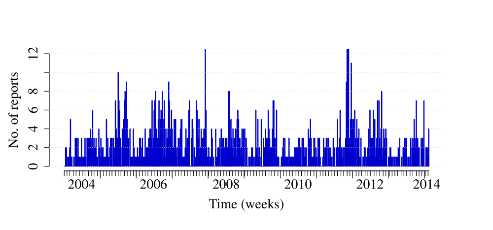
Figure 1: Weekly number of cases of S. Newport in Germany, 2004-2013.

Basic manipulation of objects of the class sts

This time series above is represented as a multivariate sts-object whose dimensions correspond to the 16 German federal states. Values are weekly counts so freq=52. Weeks are here handled as Date objects by setting epochAsDate to TRUE. One can thus for instance get the weekday of the date by calling weekdays(salmNewport). Furthermore, one can use the function format (and the package specific platform independent version dateFormat) to obtain strftime compatible formatting of the epochs. Another advantage of using Date objects is that the plot functions have been re-written for better management of ticks and labelling of the x-axis based on strtime compatible conversion specifications. For example, to get ticks at all weeks corresponding to the first week in a month as well as all weeks corresponding to the first in a year while placing labels consisting of the year at the median index per year:

R> plot(salmNewport, xaxis.tickFreq = list("%V" = atChange, "%m" = atChange, "%G" = atChange), xaxis.labelFreq = list("%Y" = atMedian), xaxis.labelFormat = "%Y", type = observed ~ time) which is shown in Fig. 1. Here, the atChange and atMedian functions are small helper functions and the respective tick lengths are controlled by the surveillance specific option surveillance.options("stsTickFactors"). Actually sts-objects can be plotted using different options: type = observed   time produces the time series for whole Germany as shown on Fig. 1, whereas type = observed   time | unit is a panelled graph with each panel representing the time series of counts of a federal state as seen on Fig. 2.

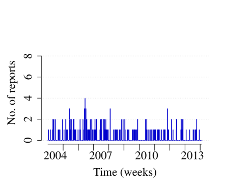
(a)

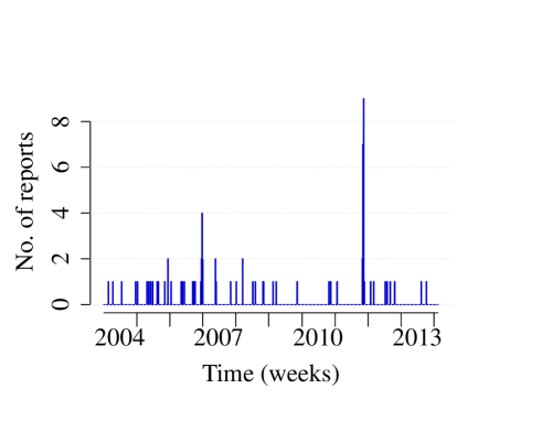
(b)

Figure 2: Weekly count of S. Newport in the German federal states (a) Bavaria and (b) Berlin.

Once created one can use typical subset operations on a sts-object: for instance salmNewport
[1:10,"Berlin"] is a new sts-object with weekly counts for Berlin during the 10 first weeks of the initial dataset; salmNewport[isoWeekYear(epoch(salmNewport))$ISOYear<=2010,] uses the surveillance’s isoWeekYear() function to get a sts-object with weekly counts for all federal states up to 2010. Moreover, one can take advantage of the R function aggregate(). For instance, aggregate(salmNewport,by="unit") returns a sts-object representing weekly counts of Salmonella Newport in Germany as a whole, whereas aggregate(salmNewport,
by="time") corresponds to the total count of cases in each federal state over the whole period.

1.2 How to use aberration detection algorithms

Monitoring algorithms in the package operate on objects of the class sts as described below.

Statistical framework for aberration detection

We introduce the framework for aberration detection on an univariate time series of counts $\left\{y_{t},\>t=1,2,\ldots\right\}$. Surveillance aims at detecting an aberration, that is to say, an important change in the process occurring at an unknown time $\tau$. This change can be a step increase of the counts of cases or a more gradual change (Sonesson and Bock, 2003).

Based on the possibility of such a change, for each time $t$ we want to differentiate between the two states in-control and out-of-control. At any timepoint $t_{0}\geq 1$, the available information – i.e., past counts – is defined as $\bm{y}_{t_{0}}=\left\{y_{t}\>;\>t\leq t_{0}\right\}$. Detection is based on a statistic $r(\cdot)$ with resulting alarm time $T_{A}=\min\left\{t_{0}\geq 1:r(\bm{y}_{t_{0}})>g\right\}$ where $g$ is a known threshold. Functions for aberration detection thus use past data to estimate $r(\bm{y}_{t_{0}})$, and compare it to the threshold $g$, above which the current count can be considered as suspicious and thus doomed as out-of-control.

Threshold values and alarm Booleans for each timepoint of the monitored range are saved in the slots upperbound and alarm, of the same dimensions as observed, while the method parameters used for computing the threshold values and alarm Booleans are stored in the slot control.

Aberration detection in the package

To perform such a monitoring of the counts of cases, one has to choose one of the surveillance algorithms of the package – this choice will be the topic of Section 2. Then, one must indicate which part of the time series or range has to be monitored – for instance the current year. Lastly, one needs to specify the parameters specific to the algorithm.

Example with the EARS C1 method

We will illustrate the basic principle by using the earsC function that implements the EARS (Early Aberration Detection System) methods of the CDC as described in Fricker et al. (2008). This algorithm is especially convenient in situations when little historic information is available. It offers three variants called C1, C2 and C3.

Here we shall expand on C1 for which the baseline are the 7 timepoints before the assessed timepoint $t_{0}$, that is to say $\left(y_{t_{0}-7},\ldots,y_{t_{0}-1}\right)$. The expected value is the mean of the baseline. The method is based on a statistic called $C_{t_{0}}$ defined as $C_{t_{0}}=\nicefrac{{(y_{t_{0}}-\bar{y}_{t_{0}})}}{{s_{t_{0}}}}$, where

$$\bar{y}_{t_{0}}=\frac{1}{7}\cdot\sum_{i=t_{0}-7}^{t_{0}-1}y_{i}\textnormal{ and }s_{t_{0}}^{2}=\frac{1}{7-1}\cdot\sum_{i=t_{0}-7}^{t_{0}-1}\left(y_{i}-\bar{y}_{t_{0}}\right)^{2}.$$

Under the null hypothesis of no outbreak, it is assumed that $C_{t_{0}}\stackrel{{\scriptstyle H_{0}}}{{\sim}}{N}(0,1)$. The upperbound $U_{t_{0}}$ is defined by a $(1-\alpha)\cdot 100\%$ confidence interval for the mean: $U_{t_{0}}=\bar{y}_{t_{0}}+z_{1-\alpha}s_{t_{0}}$ where $z_{1-\alpha}$ is the $(1-\alpha)$’th quantile of the standard normal distribution. An alarm is raised if $y_{t_{0}}>U_{t_{0}}$.

The output of the algorithm is a sts-object that contains subsets of slots observed, population and state defined by the range of timepoints specified in the input – e.g the last 20 timepoints of the timeseries, and with the slots upperbound and alarm filled by the output of the algorithm. Information relative to the range of data to be monitored and to the parameters of the algorithm, such as alpha for earsC, has to be formulated in the slot control. This information is also stored in the slot control of the returned sts-object for later inspection.

R> in2011 <- which(isoWeekYear(epoch(salmNewport))$ISOYear == 2011)R> salmNewportGermany <- aggregate(salmNewport, by = "unit")R> control <- list(range = in2011, method = "C1", alpha = 0.05)R> surv <- earsC(salmNewportGermany, control = control)R> plot(surv)

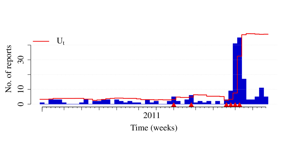
Figure 3: Weekly reports of S. Newport in Germany in 2011 monitored by the EARS C1 method. The line represents the upperbound calculated by the algorithm. Triangles indicate alarms that are the timepoints where the observed number of counts is higher than the upperbound.

The sts-object is easily visualized using the function plot as depicted in Fig. 3, which shows the upperbound as a dashed line and the alarms – timepoints where the upperbound has been exceeded – as triangles. The four last alarms correspond to a known outbreak in 2011 due to sprouts (Bayer et al., 2014). One sees that the upperbound right after the outbreak is affected by the outbreak: it is very high, so that a smaller outbreak would not be detected.

The EARS methods C1, C2 and C3 are simple in that they only use information from the very recent past. This is appropriate when data has only been collected for a short time or when one expects the count to be fairly constant. However, data from the less recent past often encompass relevant information about e.g., seasonality and time trend, that one should take into account when estimating the expected count and the associated threshold. For instance, ignoring an increasing time trend could decrease sensitivity. Inversely, overlooking an annual surge in counts during the summer could decrease specificity. Therefore, it is advisable to use detection methods whose underlying models incorporate essential characteristics of time series of disease count data such as overdispersion, seasonality, time trend and presence of past outbreaks in the records (Unkel et al., 2012; Shmueli and Burkom, 2010). Moreover, the EARS methods do not compute a proper prediction interval for the current count. Sounder statistical methods will be reviewed in the next section.

2 Using surveillance in selected contexts

More than a dozen algorithms for aberration detection are implemented in the package. Among those, this section presents a set of representative algorithms, which are already in routine application at several public health institutions or which we think have the potential to become so. First we describe the Farrington method introduced by Farrington et al. (1996) together with the improvements proposed by Noufaily et al. (2012). As a Bayesian counterpart to these methods we present the BODA method published by Manitz and Höhle (2013) which allows the easy integration of covariates. All these methods perform one-timepoint detection in that they detect aberrations only when the count at the currently monitored timepoint is above the threshold. Hence, no accumulation of evidence takes place. As an extension, we introduce an implementation of the negative binomial cumulative sum (CUSUM) of Höhle and Paul (2008) that allows the detection of sustained shifts by accumulating evidence over several timepoints. Finally, we present a method suitable for categorical data described in Höhle (2010) that is also based on cumulative sums.

2.1 One size fits them all for count data

Two implementations of the Farrington method, which is currently the method of choice at European public health institutes (Hulth et al., 2010), exist in the package. First, the original method as described in  Farrington et al. (1996) is implemented as function farrington. Its use was already described in Höhle and Mazick (2010). Now, the newly implemented function farringtonFlexible supports the use of this original method as well as of the improved method built on suggestions made by Noufaily et al. (2012) for improving the specificity without reducing the sensitivity.

In the function farringtonFlexible one can choose to use the original method or the improved method by specification of appropriate control arguments. Which variant of the algorithm is to be used is determined by the contents of the control slot. In the example below, control1 corresponds to the use of the original method and control2 indicates the options for the improved method.

R> control1 <- list(range = in2011, noPeriods = 1,                  b = 4, w = 3, weightsThreshold = 1,                  pastWeeksNotIncluded = 3, pThresholdTrend = 0.05,                  thresholdMethod = "delta")R> control2 <- list(range = in2011, noPeriods = 10,                  b = 4, w = 3, weightsThreshold = 2.58,                  pastWeeksNotIncluded = 26, pThresholdTrend = 1,                  thresholdMethod = "nbPlugin")

In both cases the steps of the algorithm are the same. In a first step, an overdispersed Poisson generalized linear model with log link is fitted to the reference data $\bm{y}_{t_{0}}\subseteq\left\{y_{t}\>;\>t\leq t_{0}\right\}$, where $\E(y_{t})=\mu_{t}$ with $\log\mu_{t}=\alpha+\beta t$ and $\operatorname{Var}(y_{t})=\phi\cdot\mu_{t}$ and where $\phi\geq 1$ is ensured.

The original method took seasonality into account by using a subset of the available data as reference data for fitting the GLM: w timepoints centred around the timepoint located $1,2,\ldots,b$ years before $t_{0}$, amounting to a total $b\cdot(2w+1)$ reference values. Yet, it was shown in Noufaily et al. (2012) that the algorithm performs better when using more historical data. In order to do do so without disregarding seasonality, the authors introduced a zero order spline with 11 knots, which can be conveniently represented as a 10-level factor. We have extended this idea in our implementation so that one can choose an arbitrary number of periods in each year. Thus, $\log\mu_{t}=\alpha+\beta t+f(t)$ where $f(t)$ is a zero order periodic spline with $\texttt{noPeriods}+1$ knots represented as a noPeriods-level factor. The algorithm uses w, b and noPeriods to deduce the length of periods so they have the same length up to rounding. An exception is the reference window centred around $t_{0}$. Figure 4 shows a minimal example, where each character corresponds to a different period. Note that setting $\texttt{noPeriods}=1$ corresponds to using the original method with only a subset of the data: there is only one period defined per year, the reference window around $t_{0}$ and other timepoints are not included in the model.

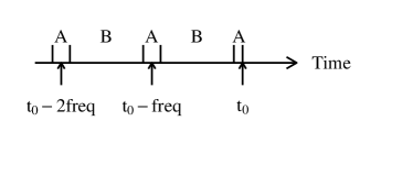
(a) $\texttt{noPeriods}=2$

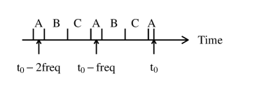
(b) $\texttt{noPeriods}=3$

Figure 4: Construction of the noPeriods-level factor to account for seasonality, depending on the value of the half-window size $w$ and of the freq of the data. Here the number of years to go back in the past $b$ is 2. Each level of the factor variable corresponds to a period delimited by ticks and is denoted by a character. The windows around $t_{0}$ are respectively of size $2w+1$, $2w+1$ and $w+1$. The segments between them are divided into the other periods so that they have the same length up to rounding.

Moreover, it was shown in Noufaily et al. (2012) that is is better to exclude the last 26 weeks before $t_{0}$ from the baseline in order to avoid reducing sensitivity when an outbreak has started recently before $t_{0}$. In the farringtonFlexible function, one controls this by specifying pastWeeksNotIncluded, which is the number of last timepoints before $t_{0}$ that are not to be used. The default value is 26.

Lastly, in the new implementation a population offset can be included in the GLM by setting populationBool to TRUE and supplying the possibly time-varying population size in the population slot of the sts-object, but this will not be discussed further here.

In a second step, the expected number of counts $\mu_{t_{0}}$ is predicted for the current timepoint $t_{0}$ using this GLM. An upperbound $U_{t_{0}}$ is calculated based on this predicted value and its variance. The two versions of the algorithm make different assumptions for this calculation. The original method assumes that a transformation of the prediction error $g\left(y_{t_{0}}-\hat{\mu}_{t_{0}}\right)$ is normally distributed, for instance when using the identity transformation $g(x)=x$ one obtains

$$y_{t_{0}}-\hat{\mu}_{0}\sim\mathcal{N}(0,\operatorname{Var}(y_{t_{0}}-\hat{\mu}_{0}))\cdot$$

The upperbound of the prediction interval is then calculated based on this distribution. First we have that

$$\operatorname{Var}(y_{t_{0}}-\hat{\mu}_{t_{0}})=\operatorname{Var}(\hat{y}_{t_{0}})+\operatorname{Var}(\hat{\mu}_{t_{0}})=\phi\mu_{0}+\operatorname{Var}(\hat{\mu}_{t_{0}})$$

with $\operatorname{Var}(\hat{y}_{t_{0}})$ being the variance of an observation and $\operatorname{Var}(\hat{\mu}_{t_{0}})$ being the variance of the estimate. The threshold, defined as the upperbound of a one-sided $(1-\alpha)\cdot 100\%$ confidence interval, is

$$U_{t_{0}}=\hat{\mu}_{0}+z_{1-\alpha}\widehat{\operatorname{Var}}(y_{t_{0}}-\hat{\mu}_{t_{0}})\cdot$$

This method can be used by setting the control option thresholdMethod equal to "delta". However, a weakness of this procedure is the normality assumption itself, so that an alternative was presented in Noufaily et al. (2012) and implemented as thresholdMethod="Noufaily". The central assumption of this approach is that $y_{t_{0}}\sim\operatorname{NB}\left(\mu_{t_{0}},\nu\right)$, with $\mu_{t_{0}}$ the mean of the distribution and $\nu=\nicefrac{{\mu_{t_{0}}}}{{\phi-1}}$ its overdispersion parameter. In this parameterization, we still have $\E(y_{t})=\mu_{t}$ and $\operatorname{Var}(y_{t})=\phi\cdot\mu_{t}$ with $\phi>1$ – otherwise a Poisson distribution is assumed for the observed count. The threshold is defined as a quantile of the negative binomial distribution with plug-in estimates $\hat{\mu}_{t_{0}}$ and $\hat{\phi}$. Note that this disregards the estimation uncertainty in $\hat{\mu}_{t_{0}}$ and $\hat{\phi}$. As a consequence, the method "muan" (mu for $\mu$ and an for asymptotic normal) tries to solve the problem by using the asymptotic normal distribution of $(\hat{\alpha},\hat{\beta})$ to derive the upper $(1-\alpha)\cdot 100\%$ quantile of the asymptotic normal distribution of $\hat{\mu}_{t_{0}}=\hat{\alpha}+\hat{\beta}t_{0}$. Note that this does not reflect all estimation uncertainty because it disregards the estimation uncertainty of $\hat{\phi}$. Note also that for time series where the variance of the estimator is large, the upperbound also ends up being very large. Thus, the method "nbPlugin" seems to provide information that is easier to interpret by epidemiologists but with "muan" being more statistically correct.

In a last step, the observed count $y_{t_{0}}$ is compared to the upperbound $U_{t_{0}}$ and an alarm is raised if $y_{t_{0}}>U_{t_{0}}$. In both cases the fitting of the GLM involves three important steps. First, the algorithm performs an optional power-transformation for skewness correction and variance stabilisation, depending on the value of the parameter powertrans in the control slot. Then, the significance of the time trend is checked. The time trend is included only when significant at a chosen level pThresholdTrend, when they are more than three years reference data and if no overextrapolation occurs because of the time trend. Lastly, past outbreaks are reweighted based on their Anscombe residuals. In farringtonFlexible the limit for reweighting past counts, weightsThreshold, can be specified by the user. If the Anscombe residuals of a count is higher than weightsThreshold it is reweighted accordingly in a second fitting of the GLM. Farrington et al. (1996) used a value of $1$ whereas Noufaily et al. (2012) advises a value of $2.56$ so that the reweighting procedure is less drastic, because it also shrinks the variance of the observations.

The original method is widely used in public health surveillance (Hulth et al., 2010). The reason for its success is primarily that it does not need to be fine-tuned for each specific pathogen. It is hence easy to implement it for scanning data for many different pathogens. Furthermore, it does tackle classical issues of surveillance data: overdispersion, presence of past outbreaks that are reweighted, seasonality that is taken into account differently in the two methods. An example of use of the function is shown on Fig. 5 with the code below.

R> salm.farrington <- farringtonFlexible(salmNewportGermany, control1)R> salm.noufaily <- farringtonFlexible(salmNewportGermany, control2)

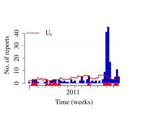
(a)

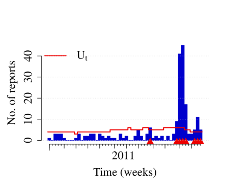
(b)

Figure 5: S. Newport in Germany in 2011 monitored by (a) the original method and (b) the improved method. For the figure we turned off the option that the threshold is only computed if there were more than 5 cases during the 4 last timepoints including $t_{0}$. One gets less alarms with the most recent method and still does not miss the outbreak in the summer. Simulations on more time series support the use of the improved method instead of the original method.

With our implementation of the improvements presented in Noufaily et al. (2012) we hope that the method with time can replace the original method in routine use. The RKI system described in section 3.2 already uses this improved method.

2.1.1 Similar methods in the package

The package also contains further methods based on a subset of the historical data: bayes, rki and cdc. See Tab. 1 for the corresponding references. Here, bayes uses a simple conjugate prior-posterior approach and computes the parameters of a negative binomial distribution based on past values. The procedure rki makes either the assumption of a normal or a Poisson distribution based on the mean of past counts. Finally, cdc aggregates weekly data into 4-week-counts and computes a normal distribution based upper confidence interval. None of these methods offers the inclusion of a linear trend, down-weighting of past outbreaks or power transformation of the data. Although these methods are good to have at hand, we personally recommend the use of the improved method implemented in the function farringtonFlexible.

2.2 A Bayesian refinement

The farringtonFlexible function described previously was a first indication that the monitoring of surveillance time series requires a good modelling of the time series before assessing aberrations. Generalized linear models (GLMs) and generalized additive models (GAMs) are well-established and powerful modelling frameworks for handling the count data nature and trends of time series in a regression context. The boda procedure (Manitz and Höhle, 2013) continues this line of thinking by extending the simple GLMs used in the farrington and farringtonFlexible procedures to a fully fledged Bayesian GAM allowing for penalized splines, e.g., to describe trends and seasonality, while simultaneously adjusting for previous outbreaks or concurrent processes influencing the case counts. A particular advantage of the Bayesian approach is that it constitutes a seamless framework for performing both estimation and subsequent prediction: the uncertainty in parameter estimation is directly carried forward to the predictive posterior distribution. No asymptotic normal approximations nor plug-in inference is needed. For fast approximate Bayesian inference we use the INLA R package (Rue et al., 2013) to fit the Bayesian GAM.

Still, monitoring with boda is substantially slower than using the Farrington procedures. Furthermore, detailed regression modelling is only meaningful if the time series is known to be subject to external influences on which information is available. Hence, the typical use at a public health institution would be the detailed analysis of a few selected time series, e.g., critical ones or those with known trend character.

As an example, Manitz and Höhle (2013) studied the influence of absolute humidity on the occurence of weekly reported campylobacter cases in Germany.

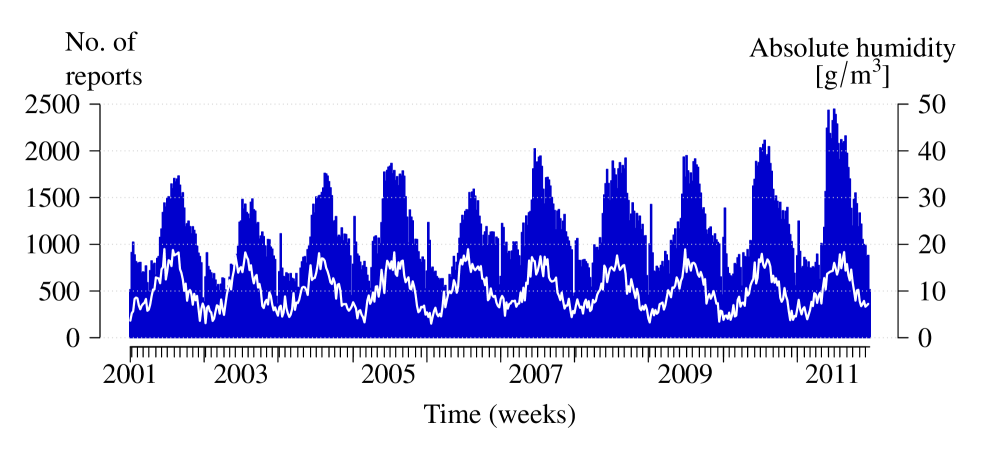
Figure 6: Weekly number of reported campylobacteriosis cases in Germany 2002-2011 as vertical bars. In addition, the corresponding mean absolute humidity time series is shown as a white curve.

R> data("campyDE")R> cam.sts <- new("sts", epoch = as.numeric(campyDE$date),                observed = campyDE$case, state = campyDE$state,                epochAsDate = TRUE)R> plot(cam.sts, legend = NULL, xlab = "time [weeks]", ylab = "No. reported",      col = "gray", cex = 2, cex.axis = 2, cex.lab = 2)R> lines(campyDE$hum * 50, col = "darkblue", lwd = 2)

The corresponding plot of the weekly time series is shown in Fig. 6. We observe a strong association between humidity and case numbers - an association which is stronger than with, e.g., temperature or relative humidity. As noted in Manitz and Höhle (2013) the excess in cases in 2007 is thus partly explained by the high atmospheric humidity. Furthermore, an increase in case numbers during the 2011 STEC O104:H4 outbreak is observed, which is explained by increased awareness and testing of many gastroenteritits pathogens during that period. The hypothesis is thus that there is no actual increased disease activity (Bernard et al., 2014). Unfortunately, the German reporting system only records positive test results without keeping track of the number of actual tests performed – otherwise this would have been a natural adjustment variable. Altogether, the series contains several artefacts which appear prudent to address when monitoring the campylobacteriosis series.

The GAM in boda is based on the negative binomial distribution with time-varying expectation and time constant overdispersion parameter, i.e.,

$$y_{t} \sim\operatorname{NB}(\mu_{t},\nu)$$

with $\mu_{t}$ the mean of the distribution and $\nu$ the dispersion parameter (Lawless, 1987). To achieve compatibility with the quasi-Poisson model we let $\phi=\nicefrac{{(\mu_{t}+\nu)}}{{\nu}}$. Hence we have $\E(y_{t})=\mu_{t}$ and $\operatorname{Var}(y_{t})=\phi\cdot\mu_{t}$ with $\phi>1$. The linear predictor is given by

$$\log(\mu_{t}) =\alpha_{0t}+\beta t+\gamma_{t}+\bm{x}_{t}^{\top}\bm{\delta}+\xi z_{t},\quad t=1,\ldots,t_{0}.$$

Here, the time-varying intercept $\alpha_{0t}$ is described by a penalized spline (e.g., first or second order random walk) and $\gamma_{t}$ denotes a periodic penalized spline (as implemented in INLA) with period equal to the periodicity of the data. Furthermore, $\beta$ characterizes the effect of a possible linear trend (on the log-scale) and $\xi$ is the effect of previous outbreaks. Typically, $z_{t}$ is a zero-one process denoting if there was an outbreak in week $t$, but more involved adaptive and non-binary forms are imaginable. Finally, $\bm{x}_{t}$ denotes a vector of possibly time-varying covariates, which influence the expected number of cases. Data from timepoints $1,\ldots,t_{0}-1$ are now used to determine the posterior distribution of all model parameters and subsequently the posterior predictive distribution of $y_{t_{0}}$ is computed. If the actual observed value of $y_{t_{0}}$ is above the $(1-\alpha)\cdot 100\%$ quantile of the predictive posterior distribution an alarm is flagged for $t_{0}$.

Below we illustrate the use of boda to monitor the campylobacterioris time series from 2007. In the first case we include in the model for $\log\left(\mu_{t}\right)$ penalized splines for trend and seasonality and a simple linear trend.

R> rangeBoda <- which(epoch(cam.sts) >= as.Date("2007-01-01"))R> control.boda <- list(range = rangeBoda, X = NULL, trend = TRUE,                      season = TRUE, prior = "iid", alpha = 0.025,                      mc.munu = 10000, mc.y = 1000)R> boda <- boda(cam.sts, control = control.boda)

In the second case we instead use only penalized and linear trend components, and, furthermore, include as covariates lags 1-4 of the absolute humidity as well as zero-one indicators for $t_{0}$ belonging to the last two weeks (christmas) or first two years (newyears) of the year, respectively. The later two variables are needed, because there is a systematically changed reporting behaviour at the turn of the year (c.f. Fig. 6). Finally, O104period is an indicator variable on whether the reporting week belongs to the W21-W30 - 2011 period of increased awareness during the O104:H4 STEC outbreak. No additional correction for past outbreaks is made.

R> covarNames <- c("l1.hum", "l2.hum", "l3.hum", "l4.hum",                 "newyears", "christmas", "O104period")R> control.boda2 <- modifyList(control.boda,                             list(X = campyDE[, covarNames], season = FALSE))R> boda.covars <- boda(cam.sts, control = control.boda2)

We plot boda.covars in Fig. 7 and compare the output of the two boda calls with the output of farrington, farringtonFlexible and bayes in Fig. 8.

R> cam.surv <- combineSTS(list(boda.covars=boda.covars,boda=boda,bayes=bayes,                             farrington=far,farringtonFlexible=farflex))R> plot(cam.surv,type = alarm ~ time)

Note here that the Bayes procedure is not really useful as the adjustment for seasonality only works poorly. Moreover, we think that this method produces many false alarms for this time series because it disregards the increasing time trend in number of reported cases. Furthermore, it becomes clear that the improved Farrington procedure acts similar to the original procedure, but the improved reweighting and trend inclusion produces fewer alarms.

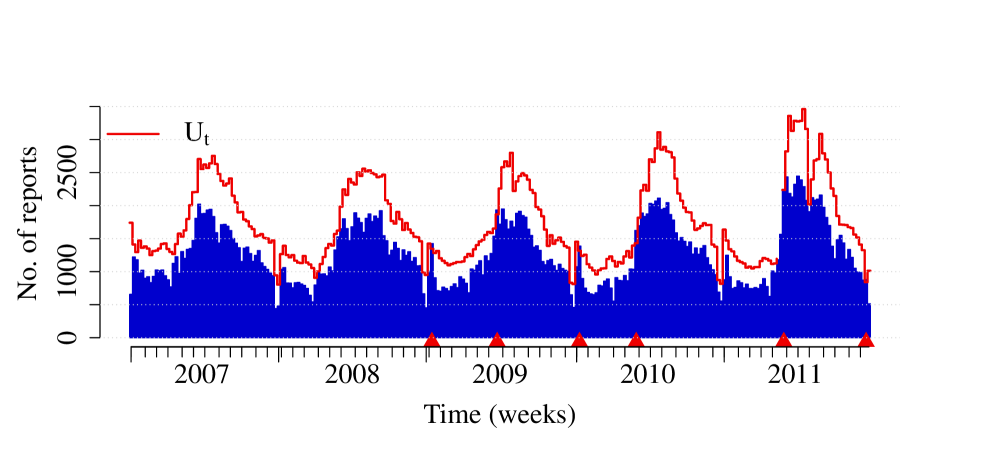
Figure 7: Weekly reports of Campylobacter in Germany in 2007-2011 monitored by the boda method with covariates. The line represents the upperbound calculated by the algorithm. Triangles indicate alarms, i.e. timepoints where the observed number of counts is higher than the upperbound.

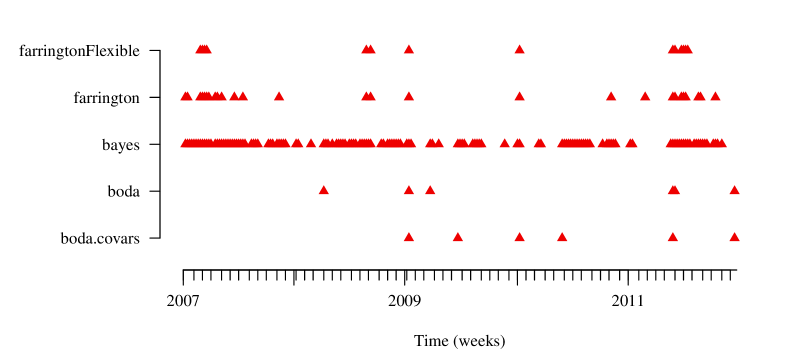
Figure 8: Alarmplot showing the alarms for the campylobacteriosis time series for four different algorithms.

2.3 Beyond one-timepoint detection

GLMs as used in the Farrington method are suitable for the purpose of aberration detection since they allow a regression approach for adjusting counts for known phenomena such as trend or seasonality in surveillance data. Nevertheless, the Farrington method only performs one-timepoint detection. In some contexts it can be more relevant to detect sustained shifts early, e.g., an outbreak could be characterized at first by counts slightly higher than usual in subsequent weeks without each weekly count being flagged by one-timepoint detection methods. Control charts inspired by statistical process control (SPC) e.g., cumulative sums would allow the detection of sustained shifts. Yet they were not tailored the specific characteristics of surveillance data such as overdispersion or seasonality. The method presented in Höhle and Paul (2008) conducts a synthesis of both worlds, i.e. traditional surveillance methods and SPC. The method is implemented in the package as the function glrnb, whose use is explained here.

2.3.1 Definition of the control chart

For the control chart, two distributions are defined, one for each of the two states in-control and out-of-control, whose likelihoods are compared at each time step. The in-control distribution $f_{\bm{\theta}_{0}}(y_{t}|\bm{z}_{t})$ with the covariates $\bm{z}_{t}$ is estimated by a GLM of the Poisson or negative binomial family with a log link, depending on the overdispersion of the data. In this context, the standard model for the in-control mean is

$$\log\mu_{0,t}=\beta_{0}+\beta_{1}t+\sum_{s=1}^{S}\left[\beta_{2s}\cos\left(\frac{2\pi st}{\texttt{Period}}\right)+\beta_{2s+1}\sin\left(\frac{2\pi st}{\texttt{Period}}\right)\right]$$

where $S$ is the number of harmonic waves to use and Period is the period of the data as indicated in the control slot, for instance 52 for weekly data. But more flexible linear predictors, e.g., containing splines, concurrent covariates or an offset could be used on the right hand-side of the equation. The GLM could therefore be made very close to the one used by Noufaily et al. (2012), with reweighting of past outbreaks and various criteria for including the time trend.

The parameters of the in-control and out-of-control models are respectively given by $\bm{\theta}_{0}$ and $\bm{\theta}_{1}$. The out-of-control mean is defined as a function of the in-control mean, either with a multiplicative shift (additive on the log-scale) whose size $\kappa$ can be given as an input or reestimated at each timepoint $t>1$, $\mu_{1,t}=\mu_{0,t}\cdot\exp(\kappa)$, or with an unknown autoregressive component as in Held et al. (2005), $\mu_{1,t}=\mu_{0,t}+\lambda y_{t-1}$ with unknown $\lambda>0$.

In glrnb, timepoints are divided into two intervals: phase 1 and phase 2. The in-control mean and overdispersion are estimated with a GLM fitted on phase 1 data, whereas surveillance operates on phase 2 data. When $\lambda$ is fixed, one uses a likelihood-ratio and defines the stopping time for alarm as

$$N=\min\left\{t_{0}\geq 1:\max_{1\leq t\leq t_{0}}\left[\sum_{s=t}^{t_{0}}\log\left\{\frac{f_{\bm{\theta}_{1}}(y_{s}|\bm{z}_{s})}{f_{\bm{\theta}_{0}}(y_{s}|\bm{z}_{s})}\right\}\right]\geq\texttt{c.ARL}\right\},$$

where $n$ is the number of timepoints in the phase 2 data and c.ARL is the threshold of the CUSUM.

When $\lambda$ is unknown and with the autoregressive component one has to use a generalized likelihood ration (GLR) with the following stopping rule to estimate them on the fly at each time point so that

$$N_{G}=\min\left\{t_{0}\geq 1:\max_{1\leq t\leq t_{0}}\sup_{\bm{\theta}\in\bm{\Theta}}\left[\sum_{s=t}^{t_{0}}\log\left\{\frac{f_{\bm{\theta}}(y_{s}|\bm{z}_{s})}{f_{\bm{\theta}_{0}}(y_{s}|\bm{z}_{s})}\right\}\right]\geq\texttt{c.ARL}\right\}\cdot$$

Thus, one does not make any hypothesis about the specific value of the change to detect, but this GLR is more computationally intensive than the LR.

2.3.2 Practical use

For using glrnb one has two choices to make. First, one has to choose an in-control model that will be fitted on phase 1 data. One can either provide the predictions for the vector of in-control means mu0 and the overdispersion parameter alpha by relying on an external fit, or use the built-in GLM estimator, that will use all data before the beginning of the surveillance range to fit a GLM with the number of harmonics S and a time trend if trend is TRUE. The choice of the exact in-control model depends on the data under surveillance. Performing model selection is a compulsory step in practical applications.

Then, one needs to tune the surveillance function itself, for one of the two possible change forms, intercept or epi. One can choose either to set theta to a given value and thus perform LR instead of GLR. The value of theta has to be adapted to the specific context in which the algorithm is applied: how big are shifts one wants to detect optimally? Is it better not to specify any and use GLR instead?

The threshold c.ARL also has to be specified by the user. As explained in Höhle and Mazick (2010) one can compute the threshold for a desired run-length in control through direct Monte Carlo simulation or a Markov chain approximation. Lastly, as mentioned in Höhle and Paul (2008), a window-limited approach of surveillance, instead of looking at all the timepoints until the first observation, can make computation faster.

Here we apply glrnb to the time series of report counts of Salmonella Newport in Germany by assuming a known multiplicative shift of factor $2$ and by using the built-in estimator to fit an in-control model with one harmonic for seasonality and a trend. This model will be refitted after each alarm, but first we use data from the years before 2011 as reference or phase1, and the data from 2011 as data to be monitored or phase2. The threshold c.ARL was chosen to be 4 as we found with the same approach as Höhle and Mazick (2010) that it made the probability of a false alarm within one year smaller than 0.1. Figure  9 shows the results of this monitoring.

R> phase1 <- which(isoWeekYear(epoch(salmNewportGermany))$ISOYear < 2011)R> phase2 <- in2011R> control = list(range = phase2, c.ARL = 4, theta = log(2), ret = "cases",                mu0 = list(S = 1, trend = TRUE, refit = FALSE))R> salmGlrnb <- glrnb(salmNewportGermany, control = control)

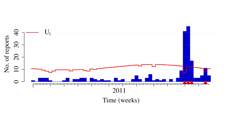
Figure 9: S. Newport in Germany in 2011 monitored by the glrnb function.

The implementation of glrnb on individual time series was already thoroughly explained in Höhle and Mazick (2010). Our objective in the present document is rather to provide practical tips for the implementation of this function on huge amounts of data in public health surveillance applications. Issues of computational speed become very significant in such a context. Our proposal to reduce the computational burden incurred by this algorithm is to compute the in-control model for each time serie (pathogen, subtype, subtype in a given location, etc.) only once a year and to use this estimation for the computation of a threshold for each time series. An idea to avoid starting with a 0 CUSUM is to use either $\left(\nicefrac{{1}}{{2}}\right)\cdot\texttt{c.ARL}$ as a starting value (fast initial response CUSUM as presented in Lucas and Crosier (1982)) or to let surveillance run with the new in-control model during a buffer period and use the resulting CUSUM as an initial value. One could also choose the maximum of these two possible starting values as a starting value. During the buffer period alarms would be generated with the old model. Lastly, using GLR is much more computationally intensive than using LR, whereas LR performs reasonably well on shifts different from the one indicated by theta as seen in the simulation studies of Höhle and Paul (2008). Our advice would therefore be to use LR with a reasonable predefined theta. The amount of historical data used each year to update the model, the length of the buffer period and the value of theta have to be fixed for each specific application, e.g. using simulations and/or discussion with experts.

2.3.3 Similar methods in the package

The algorithm glrPois is the same function as glrnb but for Poisson distributed data. Other CUSUM methods for count data are found in the package: cusum and rogerson. Both methods are discussed and compared to glrnb in Höhle and Paul (2008). The package also includes a semi-parametric method outbreakP that aims at detecting changes from a constant level to a monotonically increasing incidence, for instance the beginning of the influenza season. See Tab. 1 for the corresponding references.

2.4 A method for monitoring categorical data

All monitoring methods presented up to now have been methods for analysing count data. Nevertheless, in public health surveillance one also encounters categorical time series which are time series where the response variable obtains one of $k\geq 2$ different categories (nominal or ordinal). When $k=2$ the time series is binary, for instance representing a specific outcome in cases such as hospitalization, death or a positive result to some diagnostic test. One can also think of applications with $k>2$ if one studies e.g., the age groups of the cases in the context of monitoring a vaccination program: vaccination targeted at children could induce a shift towards older cases which one wants to detect as quickly as possible – this will be explained thorougly with an example.

The developments of prospective surveillance methods for such categorical time series were up to recently limited to CUSUM-based approaches for binary data such as those explained in Chen (1978), Reynolds and Stoumbos (2000) and Rogerson and Yamada (2004). Other than being only suitable for binary data these methods have the drawback of not handling overdispersion. A method improving on these two limitations while casting the problem into a more comprehending GLM regression framework for categorical data was presented in Höhle (2010). It is implemented as the function categoricalCUSUM.

The way categoricalCUSUM operates is very similar to what glrnb does with fixed out-of-control parameter. First, the parameters in a multivariate GLM for the in-control distribution are estimated from the historical data. Then the out-of-control distribution is defined by a given change in the parameters of this GLM, e.g., an intercept change, as explained later. Lastly, prospective monitoring is performed on current data using a likelihood ratio detector which compares the likelihood of the response under the in-control and out-of-control distributions.

2.4.1 Categorical CUSUM for Binomial Models

The challenge when performing these steps with categorical data from surveillance systems is finding an appropriate model. Binary GLMs as presented in Chapter 6 of Fahrmeir et al. (2013) could be a solution but they do not tackle well the inherent overdispersion in the binomial time series. Of course one could choose a quasi family but these are not proper statistical distributions making many issues such as prediction complicated. A better alternative is offered by the use of generalized additive models for location, scale and shape (GAMLSS) (Rigby and Stasinopoulos, 2005), that support distributions such as the beta-binomial distribution, suitable for overdispersed binary data. With GAMLSS one can model the dependency of the mean – location – upon explanatory variables but the regression modelling is also extended to other parameters of the distribution, e.g. scale. Moreover any modelled parameter can be put under surveillance, be it the mean (as in the example later developed) or the time trend in the linear predictor of the mean. This very flexible modelling framework is implemented in R through the gamlss package (Stasinopoulos and Rigby, 2007).

As an example we consider the time series of the weekly number of hospitalized cases among all Salmonella cases in Germany in Jan 2004-Jan 2014, depicted on Fig. 10. We use 2004-2012 data to estimate the in-control parameters and then perform surveillance on the data from 2013 and early 2014. We start by preprocessing the data.

R> data("salmHospitalized")R> isoWeekYearData <- isoWeekYear(epoch(salmHospitalized))R> dataBefore2013 <- which(isoWeekYearData$ISOYear < 2013)R> data2013 <- which(isoWeekYearData$ISOYear == 2013)R> dataEarly2014 <- which(isoWeekYearData$ISOYear == 2014                       & isoWeekYearData$ISOWeek <= 4)R> phase1 <- dataBefore2013R> phase2 <- c(data2013, dataEarly2014)R> weekNumbers <- isoWeekYearData$ISOWeekR> salmHospitalized.df <- cbind(as.data.frame(salmHospitalized), weekNumbers)R> colnames(salmHospitalized.df) <- c("y", "t", "state", "alarm", "n",                                    "freq", "epochInPeriod", "weekNumber")

We assume that the number of hospitalized cases follows a beta-binomial distribution, i.e., $y_{t}\sim\operatorname{BetaBin}(n_{t},\pi_{t},\sigma_{t})$ with $n_{t}$ the total number of reported cases at time $t$, $\pi_{t}$ the proportion of these cases that were hospitalized and $\sigma$ the dispersion parameter. In this parametrization,

$$E(y_{t})=n_{t}\pi_{t},\quad\text{and}$$

$$\operatorname{Var}(y_{t})=n_{t}\pi_{t}(1-\pi_{t})\left(1+\frac{\sigma(n_{t}-1)}{\sigma+1}\right)\cdot$$

We choose to model the expectation $n_{t}\pi_{t}$ using a beta-binomial model with a logit-link which is a special case of a GAMLSS, i.e.,

$$\operatorname{logit}(\pi_{t})=\bm{z}_{t}^{\top}\bm{\beta}$$

where $\bm{z}_{t}$ is a vector of possibly time-varying covariates and $\bm{\beta}$ a vector of covariate effects in our example.

The proportion of hospitalized cases varies throughout the year as seen in Fig. 10. One observes that in the summer the proportion of hospitalized cases is smaller than in other seasons. However, over the holidays in December the proportion of hospitalized cases increases. Note that the number of non-hospitalized cases drops while the number of hospitalized cases remains constant (data not shown): this might be explained by the fact that cases that are not serious enough to go to the hospital are not seen by general practitioners because sick workers do not need a sick note during the holidays. Therefore, the in-control model should contain these elements, as well as the fact that there is an increasing trend of the proportion because GPs prescribe less and less stool diagnoses so that more diagnoses are done on hospitalized cases.

We choose a model with an intercept, a time trend, two harmonic terms and a factor variable for the first two weeks of each year. The variable epochInPeriod takes into account the fact that not all years have 52 weeks.

R> vars <- c( "y", "n", "t", "epochInPeriod", "weekNumber")R> m.bbin <- gamlss(cbind(y, n-y) ~ 1 + t                  + sin(2 * pi * epochInPeriod) + cos(2 * pi * epochInPeriod)                  + sin(4 * pi * epochInPeriod) + cos(4 * pi * epochInPeriod)                  + I(weekNumber == 1) + I(weekNumber == 2),                  sigma.formula =~ 1,                  family = BB(sigma.link = "log"),                  data = salmHospitalized.df[phase1, vars])

The change we aim to detect is defined by a multiplicative change of odds, from $\nicefrac{{\pi_{t}^{0}}}{{(1-\pi_{t}^{0})}}$ to $R\cdot\nicefrac{{\pi_{t}^{0}}}{{(1-\pi_{t}^{0})}}$ with $R>0$, similar to what was done in Steiner et al. (1999) for the logistic regression model. This is equivalent to an additive change of the log-odds,

$$\operatorname{logit}(\pi_{t}^{1})=\operatorname{logit}(\pi_{t}^{0})+\log R$$

with $\pi_{t}^{0}$ being the in-control proportion and $\pi_{t}^{1}$ the out-of-control distribution. The likelihood ratio based CUSUM statistic is now defined as

$$C_{t_{0}}=\max_{1\leq t\leq{t_{0}}}\left(\sum_{s=t}^{t_{0}}\log\left(\frac{f(y_{s};\bm{z}_{s},\bm{\theta}_{1})}{f(y_{s};\bm{z}_{s},\bm{\theta}_{0})}\right)\right)$$

with $\bm{\theta}_{0}$ and $\bm{\theta}_{1}$ being the vector in- and out-of-control parameters, respectively. Given a threshold h, an alarm is sounded at the first time when $C_{t_{0}}>\texttt{h}$.

We set the parameters of the categoricalCUSUM to optimally detect a doubling of the odds in 2013 and 2014, i.e. $R=2$. Furthermore, we for now set the threshold of the CUSUM at $h=2$. We use the GAMLSS to predict the mean of the in-control and out-of-control distributions and store them into matrices with two columns among which the second one represents the reference category.

R> R <- 2R> h <- 2R> pi0 <- predict(m.bbin, newdata = salmHospitalized.df[phase2, vars],                type = "response")R> pi1 <- plogis(qlogis(pi0) + log(R))R> pi0m <- rbind(pi0, 1 - pi0)R> pi1m <- rbind(pi1, 1 - pi1) Note that the categoricalCUSUM function is constructed to operate on the observed slot of sts-objects which have as columns the number of cases in each category at each timepoint, i.e., each row of the observed slot contains the elements $(y_{t1},...,y_{tk})$.

R> populationHosp <- cbind(population(salmHospitalized),                         population(salmHospitalized))R> observedHosp <- cbind(observed(salmHospitalized),                       population(salmHospitalized) -   observed(salmHospitalized))R> nrowHosp <- nrow(salmHospitalized)R> salmHospitalized.multi <- new("sts", freq = 52, start = c(2004, 1),                               epoch = as.numeric(epoch(salmHospitalized)),                               epochAsDate = TRUE,                               observed = observedHosp,                               populationFrac = populationHosp,                               state = matrix(0, nrow = nrowHosp, ncol = 2),                               multinomialTS = TRUE) Furthermore, one needs to define a wrapper for the distribution function in order to have a argument named "mu" in the function.

R> dBB.cusum <- function(y, mu, sigma, size, log = FALSE) {  return(dBB(if (is.matrix(y)) y[1, ] else y, if (is.matrix(y)) mu[1, ] else mu, sigma = sigma, bd = size, log = log)) }

After these preliminary steps, the monitoring can be performed.

R> controlCat <- list(range = phase2, h = 2, pi0 = pi0m, pi1 = pi1m,                 ret = "cases", dfun = dBB.cusum)R> salmHospitalizedCat <- categoricalCUSUM(salmHospitalized.multi,                                         control = controlCat,                                         sigma = exp(m.bbin$sigma.coef)) The results can be seen in Fig. 11(a). With the given settings, there are alarms at week 16 in 2004 and at week 3 in 2004. The one in 2014 corresponds to the usual peak of the beginning of the year, which was larger than expected this year, maybe because the weekdays of the holidays were particularly worker-friendly so that sick notes were even less needed.

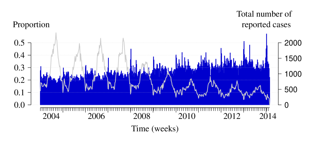
Figure 10: Weekly proportion of Salmonella cases that were hospitalized in Germany 2004-2014. In addition the corresponding number of reported cases is shown as a light curve.

The value for the threshold h can be determined following the procedures presented in Höhle and Mazick (2010) for count data, and as in the code exhibited below. Two methods can be used for determining the probability of a false alarm within a pre-specified number of steps for a given value of the threshold h: a Monte Carlo method relying on e.g., 1000 simulations and a Markov Chain approximation of the CUSUM. The former is much more computationally intensive than the latter: with the code below, the Monte Carlo method needed approximately 300 times more time than the Markov Chain method. Since both results are close we recommend the Markov Chain approximation for practical use. The Monte Carlo method works by sampling observed values from the estimated distribution and performing monitoring with categoricalCUSUM on this sts-object. As observed values are estimated from the in-control distribution every alarm thus obtained is a false alarm so that the simulations allow to estimate the probability of a false alarm when monitoring in-control data over the timepoints of phase2. The Markov Chain approximation introduced by Brook and Evans (1972) is implemented as LRCUSUM.runlength which is already used for glrnb. Results from both methods can be seen on figure 11(b). We chose a value of 2 for h so that the probability of a false alarm within the 56 timepoints of phase2 is less than $0.1$.

One first has to set the values of the threshold to be investigated and to prepare the function used for simulation, that draws observed values from the in-control distribution and performs monitoring on the corresponding time series, then indicating if there was at least one alarms. Then 1000 simulations were performed with a fixed seed value for the sake of reproducibility. Afterwards, we tested the Markov Chain approximation using the function LRCUSUM.runlength over the same grid of values for the threshold.

R> h.grid <- seq(1, 10, by = 0.5)R> simone <- function(sts, h) {   y <- rBB(length(phase2), mu = pi0m[1, , drop = FALSE],  bd = population(sts)[phase2, ],          sigma = exp(m.bbin$sigma.coef))   observed(sts)[phase2, ] <- cbind(y, sts@populationFrac[phase2, 1] - y)   one.surv <- categoricalCUSUM(sts, modifyList(controlCat, list(h = h)),                            sigma = exp(m.bbin$sigma.coef))   return(any(alarms(one.surv)[, 1])) }R> set.seed(123)R> nSims <- 1000R> pMC <- sapply(h.grid, function(h) { mean(replicate(nSims, simone(salmHospitalized.multi, h))) })R> pMarkovChain <- sapply( h.grid, function(h) {   TA <- LRCUSUM.runlength(mu = pi0m[1,, drop = FALSE],                           mu0 = pi0m[1,, drop = FALSE],                           mu1 = pi1m[1,, drop = FALSE],                           n = population(salmHospitalized.multi)[phase2, ],                           h = h, dfun = dBB.cusum,                           sigma = exp(m.bbin$sigma.coef))   return(tail(TA$cdf, n = 1)) })

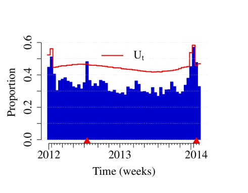
(a)

(b)

Figure 11: (a) Results of the monitoring with categoricalCUSUM of the proportion of Salmonella cases that were hospitalized in Germany in Jan 2013 - Jan 2014. (b) Probability of a false alarm within the 56 timepoints of the monitoring as a function of the threshold $h$.

The procedure for using the function for multicategorical variable follows the same steps (as illustrated later). Moreover, one could expand the approach to utilize the multiple regression possibilities offered by GAMLSS. Here we chose to try to detect a change in the mean of the distribution of counts but as GAMLSS provides more general regression tools than GLM we could also aim at detecting a change in the time trend included in the model for the mean.

2.4.2 Categorical CUSUM for Multinomial Models

In order to illustrate the use of categoricalCUSUM for more than two classes we analyse the monthly number of rotavirus cases in the federal state Brandenburg during 2002-2013 and which are stratified into the five age-groups 00-04, 05-09, 10-14, 15-69, 70+ years. In 2006 two rotavirus vaccines were introduced, which are administered in children at the age of 4-6 months. Since then, coverage of these vaccination has steadily increased and interest is to detect possible age-shifts in the distribution of cases.

R> data("rotaBB")R> plot(rotaBB, xlab = "Time (months)",      ylab = "Proportion of reported cases")

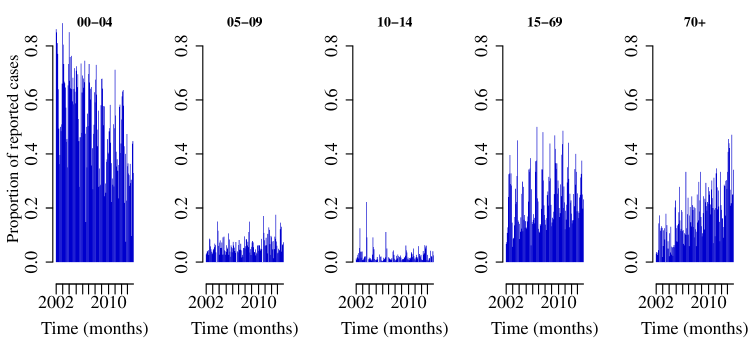
Figure 12: Monthly proportions in five age-groups for the reported rotavirus cases in Brandenburg, Germany, 2002-2013.

From Fig. 12 we observe a shift in proportion away from the very young. However, interpreting the proportions only makes sense in combination with the absolute numbers. In these plots (not shown) it becomes clear that the absolute numbers in the 0-4 year old have decreased since 2009. However, in the 70+ group a small increase is observed with 2013 by far being the strongest season so far. Hence, our interest is in prospectively detecting a possible age-shift. Since the vaccine was recommended for routine vaccination in Brandenburg in 2009 we choose to start the monitoring at that time point. We do so by fitting a multinomial logit-model containing a trend as well as one harmonic wave and use the age group 0-4 years as reference category, to the data from the years 2002-2008. Different R packages implement such type of modelling, but we shall use the MGLM package Zhang and Zhou (2014), because it also offers the fitting of extended multinomial regression models allowing for extra dispersion.

R> rotaBB.df <- as.data.frame(rotaBB)R> X <- with(rotaBB.df, cbind(intercept = 1, epoch,                            sin1 = sin(2 * pi * epochInPeriod),                            cos1 = cos(2 * pi * epochInPeriod)))R> phase1 <- epoch(rotaBB) < as.Date("2009-01-01")R> phase2 <- !phase1R> order <- c(2:5, 1); reorder <- c(5, 1:4)R> library("MGLM")R> m0 <- MGLMreg(as.matrix(rotaBB.df[phase1, order]) ~ -1 + X[phase1, ],               dist = "MN")

As described in Höhle (2010) we can try to detect a specific shift in the intercept coefficients of the model. For example, a multiplicative shift of factor 7 in the example below, in the odds of each of the four age categories against the reference category is modelled by changing the intercept value of each category. Based on this, the in-control and out-of-control proportions are easily computed using the predict function for MGLMreg objects.

R> m1 <- m0R> m1$coefficients[1, ] <- m0$coefficients[1, ] + log(7)R> pi0 <- t(predict(m0, newdata = X[phase2, ])[, reorder])R> pi1 <- t(predict(m1, newdata = X[phase2,])[, reorder])

For applying the categoricalCUSUM function one needs to define a compatible wrapper function for the multinomial as in the binomial example.

With $\bm{\pi}^{0}$ and $\bm{\pi}^{1}$ in place one only needs to define a wrapper function, which defines the PMF of the sampling distribution – in this case the multinomial – in a categoricalCUSUM compatible way.

R> dfun <- function(y, size, mu, log = FALSE) { return(dmultinom(x = y, size = size, prob = mu, log = log)) }R> control <- list(range = seq(nrow(rotaBB))[phase2], h = h, pi0 = pi0, pi1 = pi1, ret = "value", dfun = dfun)R> surv <- categoricalCUSUM(rotaBB,control=control)

The resulting CUSUM statistic $C_{t}$ as a function of time is shown in Fig. 13(a). The first time an aberration is detected is July 2009. Using 10000 Monte Carlo simulations we estimate that with the chosen threshold $h=2$ the probability for a false alarm within the 60 time points of phase2 is 0.02.

As the above example shows, the LR based categorical CUSUM is rather flexible in handling any type of multivariate GLM modelling to specify the in-control and out-of-control proportions. However, it requires a direction of the change to be specified – for which detection is optimal. One sensitive part of such monitoring is the fit of the multinomial distribution to a multivariate time series of proportions, which usually exhibit extra dispersion when compared to the multinomial. For example comparing the AIC between the multinomial logit-model and a Dirichlet-multinomial model with $\alpha_{ti}=\exp(\bm{x}_{t}^{\top}\bm{\beta})$ (Zhang and Zhou, 2014) shows that overdispersion is present. The Dirichlet distribution is the multicategorical equivalent of the beta-binomial distribution. We exemplify its use in the code below.

R> m0.dm <- MGLMreg(as.matrix(rotaBB.df[phase1, 1:5]) ~ -1 + X[phase1, ],                 dist = "DM")R> c(m0$AIC, m0.dm$AIC)

[1] 2485.446 2060.532

Hence, the above estimated false alarm probability might be too low for the actual monitoring problem, because the variation in the time series is larger than implied by the multinomial. Hence, it appears prudent to repeat the analysis using the more flexible Dirichlet-multinomial model. This is straightforward with categoricalCUSUM once the out-of-control proportions are specified in terms of the model. Such a specification is, however, hampered by the fact that the two models use different parametrizations.

For performing monitoring in this new setting we first need to calculate the $\alpha$’s of the multinomial-Dirichlet for the in-control and out-of-control distributions.

R> delta <- 2R> m1.dm <- m0.dmR> m1.dm$coefficients[1, ] <- m0.dm$coefficients[1, ] +                            c(-delta, rep(delta/4, 4))R> alpha0 <- exp(X[phase2,] %*% m0.dm$coefficients)R> alpha1 <- exp(X[phase2,] %*% m1.dm$coefficients)R> dfun <- function(y, size, mu, log = FALSE) { dLog <- ddirm(t(y), t(mu)) if (log) { return(dLog) } else { return(exp(dLog)) } }R> h <- 2R> control <- list(range = seq(nrow(rotaBB))[phase2], h = h,                 pi0 = t(alpha0), pi1 = t(alpha1),                 ret = "value", dfun = dfun)R> surv.dm <- categoricalCUSUM(rotaBB, control = control)

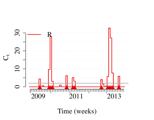
(a)

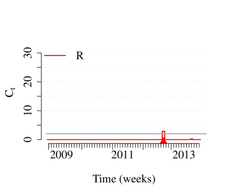
(b)

Figure 13: Categorical CUSUM statistic $C_{t}$. Once $C_{t}>2$ an alarm is sounded and the statistic is reset. In (a) surveillance uses the multinomial distribution and in (b) surveillance uses the Dirichlet-multinomial distribution.

The resulting CUSUM statistic $C_{t}$ using the Dirichlet multinomial distribution is shown in Fig. 13(b). We notice a rather similar behaviour even though the shift-type specified by this model is slightly different than in the model of Fig. 13(a).

2.4.3 Categorical data in routine surveillance

The multidimensionality of data available in public health surveillance creates many opportunities for the application of categorical time series: one could e.g., look at the sex ratio of cases of a given disease, at the age categories distribution, at the regions sending data, etc. If one is interested in monitoring with respect to a categorical variable, a choice has to be made between monitoring each time series individually, for instance a time series of Salmonella cases for each age category, or to monitor the distribution of cases with respect to that factor via categoricalCUSUM. A downside of the latter solution is that one has to specify the change parameter R in advance. However, more straightforward applications could be found in the surveillance of positive diagnostics if one were to obtain data about tests performed by laboratories and not only about confirmed cases. An alternative would be to apply farringtonFlexible while using the number of tests as populationOffset.

2.4.4 Similar methods in the package

The package also offers another CUSUM method suitable for binary data, pairedbinCUSUM that implements the method introduced by Steiner et al. (1999), which does not, however, take overdispersion into account as well as glrnb. The algorithm rogerson also supports the analysis of binomial data. See Tab. 1 for the corresponding references.

2.5 Other algorithms implemented in the package

We conclude this description of surveillance methods by giving an overview of all algorithms implemented in the package with the corresponding references in Tab. 1. One can refer to the relative reference articles and to the reference manual of the package for more information about each method.

Criteria for choosing a method in practice are numerous. First one needs to ponder on the amount of historical data at hand – for instance the EARS methods only need data for the last timepoints whereas the Farrington methods use data up to $b$ years in the past. Then one should consider the amount of past data used by the algorithm – historical reference methods use only a subset of the past data, namely the timepoints located around the same timepoint in the past years, whereas other methods use all past data included in the reference data. This can be a criterion of choice since one can prefer using all available data. It is also important to decide whether one wants to detect one-timepoint aberration or more prolonged shifts. And lastly, an important criteria is how much work needs to be done for finetuning the algorithm for each specific time series.

The package on the one hand provides the means for analysing nearly all type of surveillance data and on the other hand makes the comparison of algorithms possible. This is useful in practical applications when those algorithms are implemented into routine use, which will be the topic of section 3.

surveillance function	References
boda	Manitz and Höhle (2013)
bayes	Riebler (2004)
categoricalCUSUM	Höhle (2010)
cdc	Stroup et al. (1989); Farrington and Andrews (2003)
cusum	Rossi et al. (1999); Pierce and Schafer (1986)
earsC	Fricker et al. (2008)
farrington	Farrington et al. (1996)
farringtonFlexible	Farrington et al. (1996); Noufaily et al. (2012)
glrnb	Höhle and Paul (2008)
glrpois	Höhle and Paul (2008)
outbreakP	Frisén et al. (2009); Frisén and Andersson (2009)
pairedbinCUSUM	Steiner et al. (1999)
rki	Not available – unpublished
rogerson	Rogerson and Yamada (2004)

Table 1: Algorithms for aberration detection implemented in surveillance.

3 Implementing surveillance in routine monitoring

Combining surveillance with other R packages and programs is easy, allowing the integration of the aberration detection into a comprehensive surveillance system to be used in routine practice. In our opinion, such a surveillance system has to at least support the following process: loading data from local databases, analysing them within surveillance and sending the results of this analysis to the end-user who is typically an epidemiologist in charge of the specific pathogen. This section exemplifies the integration of the package into a whole analysis stack, first through the introduction of a simple workflow from data query to a Sweave report of signals, and secondly through the presentation of the more elaborate system in use at the German Robert Koch Institute.

3.1 A simple surveillance system

Suppose you have a database with surveillance time series but little resources to build a surveillance system encompassing all the above stages. Using R and Sweave for LaTeX you can still set up a simple surveillance analysis without having to do everything by hand. You only need to input the data into R and create sts-objects for each time series of interest as explained thoroughly in Höhle and Mazick (2010). Then, after choosing a surveillance algorithm, say farringtonFlexible, and feeding it with the appropriate control argument, you can get a sts-object with upperbounds and alarms for each of your time series of interest over the range supplied in control. For defining the range automatically one could use the R-function SysDate() to get today’s date. These steps can be introduced as a code chunk in a Sweave code that will translate it into a report that you can send to the epidemiologists in charge of the respective pathogen whose cases are monitored.

Below is an example of a short code segment showing the analysis of the S. Newport weekly counts of cases in the German federal states Baden-Württemberg and North Rhine-Westphalia with the improved method implemented in farringtonFlexible. The package provides a toLatex method for sts objects that produces a table with the observed number of counts and upperbound for each column in observed, where alarms can be highlighted by for instance bold text. The resulting table is shown in Tab. 2.

R> data("salmNewport")R> today <- which(epoch(salmNewport) == as.Date("2013-12-23"))R> rangeAnalysis <- (today - 4):todayR> in2013 <- which(isoWeekYear(epoch(salmNewport))$ISOYear == 2013)R> algoParameters <- list(range = rangeAnalysis, noPeriods = 10,                        populationBool = FALSE,                        b = 4, w = 3, weightsThreshold = 2.58,                        pastWeeksNotIncluded = 26, pThresholdTrend = 1,                        thresholdMethod = "nbPlugin", alpha = 0.05,                        limit54 = c(0, 50))R> results <- farringtonFlexible(salmNewport[, c("Baden.Wuerttemberg",                                              "North.Rhine.Westphalia")],                   control = algoParameters)R> start <- isoWeekYear(epoch(salmNewport)[range(range)[1]])R> end <- isoWeekYear(epoch(salmNewport)[range(range)[2]])R> caption <- paste("Results of the analysis of reported S. Newport                  counts in two German federal states for the weeks W-",                  start$ISOWeek, "-", start$ISOYear, " - W-", end$ISOWeek,                  "-", end$ISOYear, " performed on ", Sys.Date(),                  ". Bold upperbounds (UB) indicate weeks with alarms.",                  sep="")R> toLatex(results, caption = caption)

Year	Week	Baden-Wuerttemberg	Threshold	North-Rhine-Westphalen	Threshold
2013	48	0	5	0	4
2013	49	1	3	0	3
2013	50	1	3	0	3
2013	51	2	3	0	3
2013	52	3	2	1	3

Table 2: Results of the analysis of reported S. Newport counts in two German federal states for the weeks W-48 2013 - W-52 2013 performed on 2014-07-29. Bold upperbounds (thresholds) indicate weeks with alarms.

The advantage of this approach is that it can be made automatic. The downside of such a system is that the report is not interactive, for instance one cannot click on the cases and get the linelist. Nevertheless, this is a workable solution in many cases – especially when human and financial resources are narrow. In the next Section, we present a more advanced surveillance system built on the package.

3.2 Automatic detection of outbreaks at the Robert Koch Institute

The package surveillance was used as a core building block for designing and implementing the automated outbreak detection system at the RKI in Germany (Schumacher et al., 2014). Due to the Infection Protection Act (IfSG) the RKI daily receives over 1,000 notifiable disease reports. The system analyses about half a million time series per day to identify possible aberrations in the reported number of cases. Structurally, it consists of two components: an analytical process written in R that daily monitors the data and a reporting component that compiles and communicates the results to the epidemiologists.

The analysis task relies on surveillance and three other R packages, namely data.table, RODBC and testthat as described in the following. The data-backend is an OLAP-system (Microsoft Corp., 2012a) and relational databases, which are queried using RODBC (Ripley and Lapsley, 2012). The case reports are then fastly aggregated into univariate time series using data.table (Dowle et al., 2013). To each time series we apply the farringtonFlexible algorithm on univariate sts-objects and store the analysis results in another SQL-database. We make intensive use of testthat (Wickham, 2013) for automatic testing of the component. Although R is not the typical language to write bigger software components for production, choosing R in combination with surveillance enabled us to quickly develop the analysis workflow. We can hence report positive experience using R also for larger software components in production.

The reporting component was realized using Microsoft Reporting Services (Microsoft Corp., 2012b), because this technology is widely used within the RKI. It allows quick development of reports and works well with existing Microsoft Office tools, which the end-user, the epidemiologist, is used to. For example, one major requirement by the epidemiologists was to have the results compiled as Excel documents. Moreover, pathogen-specific reports are automatically sent once a week by email to epidemiologists in charge of the respective pathogen.

Having state-of-the-art detection methods already implemented in surveillance helped us to focus on other challenges during development, such as bringing the system in the organization’s workflow and finding ways to efficiently and effectively analyse about half a million of time series per day. In addition, major developments in the R component can be shared with the community and are thus available to other public health institutes as well.

Discussion

The R package surveillance was initially created as an implementational framework for the development and the evaluation of outbreak detection algorithms in routine collected public health surveillance data. Throughout the years it has more and more also become a tool for the use of surveillance in routine practice. The presented description aimed at showing the potential of the package for aberration derection. Other functions offered by the package for modelling (Meyer et al., 2014) or back-projection of incidence cases (Becker and Marschner, 1993) are documented elsewhere and contribute to widening the scope of possible analysis in infectious disease epidemiology when using surveillance. Future areas of interest for the package are e.g., to better take into account the multivariate and hierarchical structure of the data streams analysed. Another important topic is the adjustment for reporting delays when performing the surveillance. The package can be obtained from CRAN and resources for learning its use are listed in the documentation section of the project. As all R packages, surveillance is distributed with a manual describing each function with corresponding examples. The manual, the present article and two previous ones (Höhle, 2007; Höhle and Mazick, 2010) form a good basis for getting started with the package. The data and analysis of the present manuscript are accessible as the vignette "monitoringCounts.Rnw" in the package.

Since all functionality is available just at the cost of learning R we hope that parts of the package can be useful in health facilities around the world. Even though the package is tailored for surveillance in public health contexts, properties such as overdispersion, low counts, presence of past outbreaks, apply to a wide range of count and categorical time series in other surveillance contexts such as financial surveillance (Frisén, 2008), occupational safety monitoring (Schuh et al., 2013) or environmental surveillance (Luo et al., 2012).

Other R packages can be worth of interest to surveillance users. Statistical process control is offered by two other packages, spc (Knoth, 2014) and qcc (Scrucca, 2004). The package strucchange allows detecting structural changes in general parametric models including GLMs (Zeileis et al., 2002). For epidemic modelling and outbreaks, packages such as EpiEstim (Cori, 2013), outbreaker (Jombart et al., 2014) and OutbreakTools (The Hackout team, 2014) offer good functionalities for investigating outbreaks that may for instance have been detected through to the use of surveillance. They are listed on the website of the R-epi project that was initiated for compiling information about R tools useful for infectious diseases epidemiology. Another software of interest for aberration detection is SaTScan (Kulldorff, 1997) which allows the detection of spatial, temporal and space-time clusters of events – note that it is not a R package.

Code contributions to the package are very welcome as well as feedback and suggestions for improving the package.

References

- Bayer et al. (2014) Bayer C, Bernard H, Prager R, Rabsch W, Hiller P, Malorny B, Pfefferkorn B, Frank C, de Jong A, Friesema I, et al. (2014). “An Outbreak of Salmonella Newport Associated with Mung Bean Sprouts in Germany and the Netherlands, October to November 2011.” Eurosurveillance, 19(1).
- Becker and Marschner (1993) Becker NG, Marschner IC (1993). “A Method for Estimating the Age-Specific Relative Risk of HIV Infection from AIDS Incidence Data.” Biometrika, 80(1).
- Bernard et al. (2014) Bernard H, Werber D, Hohle M (2014). “Estimating the under-reporting of norovirus illness in Germany utilizing enhanced awareness of diarrhoea during a large outbreak of Shiga toxin-producing E. coli O104:H4 in 2011 - a time series analysis.” BMC Infectious Diseases, 14(1), 116. 10.1186/1471-2334-14-116.
- Bivand et al. (2013) Bivand RS, Pebesma E, Gomez-Rubio V (2013). Applied Spatial Data Analysis With \proglangR, Second Edition. Springer-Verlag.
- Brook and Evans (1972) Brook D, Evans DA (1972). “An Approach to the Probability Distribution of Cusum Run Length.” Biometrika, 59(3), 539–549.
- Buckeridge et al. (2005) Buckeridge DL, Burkom H, Campbell M, Hogan WR, Moore AW (2005). “Algorithms for Rapid Outbreak Detection: a Research Synthesis.” Journal of Biomedical Informatics, 38(2), 99 – 113. ISSN 1532-0464. http://dx.doi.org/10.1016/j.jbi.2004.11.007.
- Chen (1978) Chen R (1978). “A Surveillance System for Congenital Malformations.” Journal of the American Statistical Association, 73(362), 323–327. 10.1080/01621459.1978.10481577.
- Cori (2013) Cori A (2013). \pkgEpiEstim: a Package to Estimate Time Varying Reproduction Numbers from Epidemic Curves. \proglangR Package Version 1.1-2, URL http://CRAN.R-project.org/package=EpiEstim.
- Dowle et al. (2013) Dowle M, Short T, Lianoglou S (2013). \pkgdata.table: Extension of \pkgdata.frame for Fast Indexing, Fast Ordered Joins, Fast Assignment, Fast Grouping and List Columns. \proglangR Package Version 1.8.8, URL http://CRAN.R-project.org/package=data.table.
- Fahrmeir et al. (2013) Fahrmeir L, Kneib T, Lang S, Marx B (2013). Regression: Models, Methods and Applications. Springer-Verlag. ISBN 978-3-642-34333-9.
- Farrington and Andrews (2003) Farrington C, Andrews N (2003). “Outbreak Detection: Application to Infectious Disease Surveillance.” In R Brookmeyer, D Stroup (eds.), Monitoring the Health of Populations, pp. 203–231. Oxford University Press.
- Farrington et al. (1996) Farrington C, Andrews N, Beale A, Catchpole M (1996). “A Statistical Algorithm for the Early Detection of Outbreaks of Infectious Disease.” Journal of the Royal Statistical Society A, 159, 547–563.
- Fricker et al. (2008) Fricker RD, Hegler BL, Dunfee DA (2008). “Comparing Syndromic Surveillance Detection Methods: EARS’ versus a CUSUM-Based Methodology.” Statistics in Medicine, 27(17), 3407–3429.
- Frisén (2008) Frisén M (2008). Financial surveillance. John Wiley & Sons.
- Frisén and Andersson (2009) Frisén M, Andersson E (2009). “Semiparametric Surveillance of Monotonic Changes.” Sequential Analysis, 28(4), 434–454.
- Frisén et al. (2009) Frisén M, Andersson E, Schiöler L (2009). “Robust Outbreak Surveillance of Epidemics in Sweden.” Statistics in Medicine, 28, 476–493.
- Held et al. (2006) Held L, Hofmann M, Höhle M, Schmid V (2006). “A Two Component Model for Counts of Infectious Diseases.” Biostatistics, 7, 422–437.
- Held et al. (2005) Held L, Höhle M, Hofmann M (2005). “A Statistical Framework for the Analysis of Multivariate Infectious Disease Surveillance Data.” Statistical Modelling, 5, 187–199.
- Höhle (2007) Höhle M (2007). “\pkgsurveillance: An \proglangR Package for the Monitoring of Infectious Diseases.” Computational Statistics, 22(4), 571–582.
- Höhle (2010) Höhle M (2010). “Online Change-Point Detection in Categorical Time Series.” In T Kneib, G Tutz (eds.), Statistical Modelling and Regression Structures, pp. 377–397. Physica-Verlag HD. 10.1007/978-3-7908-2413-1_20.
- Höhle and Mazick (2010) Höhle M, Mazick A (2010). “Aberration Detection in \proglangR Illustrated by Danish Mortality Monitoring.” In T Kass-Hout, X Zhang (eds.), Biosurveillance: A Health Protection Priority, chapter 12, pp. 215–238. CRC Press.
- Höhle and Paul (2008) Höhle M, Paul M (2008). “Count Data Regression Charts for the Monitoring of Surveillance Time Series.” Computational Statistics & Data Analysis, 52(9), 4357–4368.
- Hulth et al. (2010) Hulth A, Andrews N, Ethelberg S, Dreesman J, Faensen D, van Pelt W, Schnitzler J (2010). “Practical Usage of Computer-Supported Outbreak Detection in Five European Countries.” Eurosurveillance, 15(36).
- Jombart et al. (2014) Jombart T, Cori A, Didelot X, Cauchemez S, Fraser C, Ferguson N (2014). “Bayesian Reconstruction of Disease Outbreaks by Combining Epidemiologic and Genomic Data.” PLoS Comput Biol, 10(1), e1003457. 10.1371/journal.pcbi.1003457.
- Knoth (2014) Knoth S (2014). \pkgspc: Statistical Process Control – Collection of Some Useful Functions. \proglangR Package Version 0.5.0, URL http://CRAN.R-project.org/package=spc.
- Kulldorff (1997) Kulldorff M (1997). \proglangSaTScan: Software for the Spatial, Temporal and Space-Time Scan Statistics. Boston, MA, USA. URL http://www.satscan.org/.
- Lawless (1987) Lawless JF (1987). “Negative Binomial and Mixed Poisson Regression.” Canadian Journal of Statistics, 15(3), 209–225.
- Lucas and Crosier (1982) Lucas JM, Crosier RB (1982). “Fast Initial Response for CUSUM Quality-Control Schemes: Give Your CUSUM a Head Start.” Technometrics, 24(3), 199–205.
- Luo et al. (2012) Luo P, DeVol TA, Sharp JL (2012). “CUSUM Analyses of Time-Interval Data for Online Radiation Monitoring.” Health physics, 102(6), 637–645.
- Manitz and Höhle (2013) Manitz J, Höhle M (2013). “Bayesian Outbreak Detection Algorithm for Monitoring Reported Cases of Campylobacteriosis in Germany.” Biometrical Journal, 55(4), 509–526. ISSN 1521-4036. 10.1002/bimj.201200141.
- Meyer et al. (2012) Meyer S, Elias J, Höhle M (2012). “A Space-Time Conditional Intensity Model for Invasive Meningococcal Disease Occurrence.” Biometrics, 68(2), 607–616.
- Meyer et al. (2014) Meyer S, Held L, Höhle M (2014). “Spatio-Temporal Analysis of Epidemic Phenomena Using the \proglangR Package \pkgsurveillance.” In preparation.
- Microsoft Corp. (2012a) Microsoft Corp (2012a). Microsoft SQL Server Analysis Services, Version 2012. URL http://www.microsoft.com/.
- Microsoft Corp. (2012b) Microsoft Corp (2012b). Microsoft SQL Server Reporting Services, Version 2012. URL http://www.microsoft.com/.
- Noufaily et al. (2012) Noufaily A, Enki D, Farrington P, Garthwaite P, Andrews N, Charlett A (2012). “An Improved Algorithm for Outbreak Detection in Multiple Surveillance Systems.” Statistics in Medicine.
- Pebesma and Bivand (2005) Pebesma EJ, Bivand RS (2005). “Classes and Methods for Spatial Data In \proglangR.” R News, 5(2), 9–13. URL http://CRAN.R-project.org/doc/Rnews/.
- Pierce and Schafer (1986) Pierce D, Schafer D (1986). “Residuals in Generalized Linear Models.” Journal of the American Statistical Association, 81(396), 977–986.
- Reynolds and Stoumbos (2000) Reynolds M, Stoumbos Z (2000). “A general approach to modeling CUSUM charts for a proportion.” IIE Transactions, 32(6), 515–535.
- Riebler (2004) Riebler A (2004). Empirischer Vergleich von statistischen Methoden zur Ausbruchserkennung bei Surveillance Daten. Master’s thesis, Department of Statistics, University of Munich. Bachelor’s thesis.
- Rigby and Stasinopoulos (2005) Rigby RA, Stasinopoulos DM (2005). “Generalized Additive Models for Location, Scale and Shape.” Journal of the Royal Statistical Society C, 54(3), 507–554. 10.1111/j.1467-9876.2005.00510.x.
- Ripley and Lapsley (2012) Ripley B, Lapsley M (2012). \pkgRODBC: ODBC Database Access. \proglangR Package Version 1.3-6, URL http://CRAN.R-project.org/package=RODBC.
- Rogerson and Yamada (2004) Rogerson P, Yamada I (2004). “Approaches to Syndromic Surveillance When Data Consist of Small Regional Counts.” Morbidity and Mortality Weekly Report, 53, 79–85.
- Rossi et al. (1999) Rossi G, Lampugnani L, Marchi M (1999). “An Approximate CUSUM Procedure for Surveillance of Health Events.” Statistics in Medicine, 18, 2111–2122.
- Rue et al. (2013) Rue H, Martino S, Lindgren F, Simpson D, Riebler A (2013). \pkgINLA: Functions Which Allow to Perform Full Bayesian Analysis of Latent Gaussian Models Using Integrated Nested Laplace Approximation. \proglangR Package Version 0.0-1386250221.
- Ryan and Ulrich (2014) Ryan JA, Ulrich JM (2014). Package \pkgxts. \proglangR Package Version 0.9-7, URL http://CRAN.R-project.org/package=xts.
- Schuh et al. (2013) Schuh A, Camelio JA, Woodall WH (2013). “Control Charts for Accident Frequency: a Motivation for Real-Time Occupational Safety Monitoring.” International Journal of Injury Control and Safety Promotion, pp. 1–9. 10.1080/17457300.2013.792285.
- Schumacher et al. (2014) Schumacher D, Salmon M, Frank C, Claus H, Höhle M (2014). “Automated outbreak detection system for notifiable diseases in Germany.” Submitted.
- Scrucca (2004) Scrucca L (2004). “\pkgqcc: an \proglangR Package for Quality Control Charting and Statistical Process Control.” R News, 4/1, 11–17. URL http://CRAN.R-project.org/doc/Rnews/.
- Shmueli and Burkom (2010) Shmueli G, Burkom H (2010). “Statistical Challenges Facing Early Outbreak Detection in Biosurveillance.” Technometrics, 52(1), 39–51. 10.1198/TECH.2010.06134.
- Sonesson and Bock (2003) Sonesson C, Bock D (2003). “A Review and Discussion of Prospective Statistical Surveillance in Public Health.” Journal of the Royal Statistical Society A, 166(1), 5–21. ISSN 1467-985X.
- Stasinopoulos and Rigby (2007) Stasinopoulos DM, Rigby RA (2007). “Generalized Additive Models for Location Scale and Shape (GAMLSS) in \proglangR.” Journal of Statistical Software, 23(7), 1–46. ISSN 1548-7660. URL http://www.jstatsoft.org/v23/i07.
- Steiner et al. (1999) Steiner SH, Cook RJ, Farewell VT (1999). “Monitoring Paired Binary Surgical Outcomes Using Cumulative Sum Charts.” Statistics in Medicine, 18, 69–86.
- Stroup et al. (1989) Stroup D, Williamson G, Herndon J, Karon J (1989). “Detection of Aberrations in the Occurrence of Notifiable Diseases Surveillance Data.” Statistics in Medicine, 8, 323–329.
- The Hackout team (2014) The Hackout team (2014). \pkgOutbreakTools: Basic Tools for the Analysis of Disease Outbreaks. \proglangR Package Version 0.1-0, URL http://CRAN.R-project.org/package=OutbreakTools.
- Unkel et al. (2012) Unkel S, Farrington CP, Garthwaite PH, Robertson C, Andrews N (2012). “Statistical Methods for the Prospective Detection of Infectious Disease Outbreaks: a Review.” Journal of the Royal Statistical Society A, 175(1), 49–82. ISSN 1467-985X. 10.1111/j.1467-985X.2011.00714.x.
- Wickham (2013) Wickham H (2013). \pkgtestthat: Testthat Code. Tools to Make Testing Fun :). \proglangR Package Version 0.7.1, URL http://CRAN.R-project.org/package=testthat.
- Zeileis and Grothendieck (2005) Zeileis A, Grothendieck G (2005). “zoo: S3 Infrastructure for Regular and Irregular Time Series.” Journal of Statistical Software, 14(6), 1–27. URL http://www.jstatsoft.org/v14/i06/.
- Zeileis et al. (2002) Zeileis A, Leisch F, Hornik K, Kleiber C (2002). “\pkgstrucchange: An \proglangR Package for Testing for Structural Change in Linear Regression Models.” Journal of Statistical Software, 7(2), 1–38. ISSN 1548-7660. URL http://www.jstatsoft.org/v07/i02.
- Zhang and Zhou (2014) Zhang Y, Zhou H (2014). \pkgMGLM: Multivariate Response Generalized Linear Models. \proglangR Package Version 0.0.4, URL http://CRAN.R-project.org/package=MGLM.