Kullback-Leibler divergence for interacting multiple model estimation with random matrices

Abstract

This paper studies the problem of interacting multiple model (IMM) estimation for jump Markov linear systems with unknown measurement noise covariance. The system state and the unknown covariance are jointly estimated in the framework of Bayesian estimation, where the unknown covariance is modeled as a random matrix according to an inverse-Wishart distribution. For the IMM estimation with random matrices, one difficulty encountered is the combination of a set of weighted inverse-Wishart distributions. Instead of using the moment matching approach, this difficulty is overcome by minimizing the weighted Kullback-Leibler divergence for inverse-Wishart distributions. It is shown that a closed form solution can be derived for the optimization problem and the resulting solution coincides with an inverse-Wishart distribution. Simulation results show that the proposed filter performs better than the previous work using the moment matching approach.

I Introduction

Jump Markov linear systems have received considerable attention due to its applications in a wide variety of signal processing systems and control systems [1, 2, 3, 4]. For discrete-time jump Markov linear systems, the dynamics are represented by a number of modes governed by a finite state Markov chain and within each mode the continuous state is described by a stochastic difference equation. Unfortunately, computing the optimal state estimate of jump Markov linear systems requires exponential complexity as time progresses. As a result, many suboptimal filters have been proposed such as the generalized pseudo Bayesian [5], the interacting multiple model (IMM) estimator [6], the particle filter [7, 8, 9] and the array algorithms [10]. See the survey for more detailed discussions on multiple model methods [11].

State estimation for jump Markov systems with unknown measurement noise statistics has been investigated in recent years. In [12], a robust extended Kalman filter (EKF) has been developed for jump Markov nonlinear systems with uncertain noise, where the uncertainty of noise covariance matrix is limited by an upper bound and the filter is derived by solving a nonlinear programming problem with inequality constraints. In [13], a linear minimum mean square error (LMMSE) estimator has been proposed for jump Markov linear systems without Gaussian assumptions on the noise and the estimator has been extended to develop an optimal polynomial filter for stochastic systems with switching measurements in [14]. In [15], a minimax filter has been derived for stochastic bimodal systems with unknown binary switching statistics. In [16], the $H_{\infty}$ filter has been combined with the IMM approach, where the purpose of the $H_{\infty}$ filter is to minimize the worst possible effects of the unknown noise to the estimation errors. In addition, some weighting parameters should be designed carefully to guarantee the existence and the performance of the $H_{\infty}$ filter.

Recently, the random matrix approach has been used for state estimation of stochastic systems with unknown measurement noise covariance [17, 18]. By using different conjugate prior distributions for the unknown measurement noise covariance, state estimation for jump Markov linear systems with unknown measurement noise covariance has been addressed in the framework of Bayesian estimation. In [19], by treating the conjugate prior for the noise variance parameters as the inverse-Gamma distribution, an IMM estimator has been developed for jump Markov linear systems. However, a serious limitation in this filter is that the noise covariance is restricted as a diagonal matrix. This assumption is used due to the fact that each diagonal element of the matrix can be modeled by an inverse-Gamma distribution but not the matrix itself. In fact, a matrix can be considered as multivariate random variable and the inverse-Wishart distribution can be used as the conjugate prior for the covariance matrix of a multivariate Gaussian distribution [20]. By using the inverse-Wishart distribution as the conjugate prior for the measurement noise covariance, an IMM estimator has been proposed in [21]. Due to the presence of the estimation of random matrices, one difficulty encountered in the IMM estimation is the combination of a set of weighted inverse-Wishart distributions. In [21], an inverse-Wishart distribution is used to approximate a set of weighted inverse-Wishart distributions by matching the first order moment and the mean squared estimation errors. However, it is not clear whether it is effective to approximate a set of weighted inverse-Wishart distributions by using the moment matching method.

In this paper, we attempt to propose a novel IMM estimator for jump Markov linear systems with unknown measurement noise covariance. By modeling the unknown measurement covariance as a random matrix according to an inverse-Wishart distribution, the state and the random matrix are estimated jointly in the framework of Bayesian estimation. Instead of using the moment matching approach to address the combination of a set of weighted inverse-Wishart distributions, this difficulty is overcome by minimizing the weighted Kullback-Leibler divergence for inverse-Wishart distributions. It is shown that a closed form solution can be derived for the optimization problem and the resulting solution coincides with an inverse-Wishart distribution. A simulation study of maneuvering target tracking is provided to illustrate the effectiveness of the proposed filter. Simulation results show that the proposed filter performs better than the previous work using the moment matching approach.

The rest of this paper is organized as follows. In section ii@, the problem of state estimation for jump Markov linear systems is formulated. In section iii@, the weighted Kullback-Leibler divergence is introduced and it is applied in the IMM approach to develop a novel estimator. A numerical example is provided in section iv@, followed by conclusions in section v@.

II Problem formulation

Consider the following jump Markov linear system

$$x_{k} =F_{k-1}(r_{k})x_{k-1}+G_{k-1}(r_{k})w_{k-1}(r_{k})$$ (1)

$$z_{k} =H_{k}x_{k}+v_{k}$$ (2)

where $x_{k}\in\mathbb{R}^{n}$ and $z_{k}\in\mathbb{R}^{m}$ denote the state and the measurement vectors, respectively. $r_{k}$ is a discrete variable denoting the state of a Markov chain and taking values in the set $\mathcal{M}\triangleq\{1,2,\cdots,M\}$ according to the transition probability matrix $\Pi=[\pi_{ij}]_{M\times M}$ with

$$\pi_{ij} \triangleq\mathbb{P}\{r_{k}=j|r_{k-1}=i\}$$ (3)

$$\sum_{n=1}^{M}\pi_{ij}=1,~{}i\in\mathcal{M}$$ (4)

The quantities $F_{k-1}(r_{k})$, $G_{k-1}(r_{k})$ and $H_{k}$ are known matrices. Note that the measurement equation (2) does not evolve with time according to the Markov state. This is a reasonable condition since the measurement is generally insensitive to the state of the model. The process noise $w_{k-1}(r_{k})$ corresponding to mode $r_{k}$ and the measurement noise $v_{k}$ are assumed to be mutually uncorrelated zero-mean white Gaussian processes with covariance matrices $Q_{k-1}(r_{k})$ and $R_{k}$, respectively. The measurement noise covariance $R_{k}$ is assumed to be unknown and it is modeled as a random matrix with the conjugate prior of an inverse-Wishart distribution [20].

The aim of this paper is to derive the estimates of the state $x_{k}$ and the random matrix $R_{k}$ in the framework of Bayesian estimation. To this end, the IMM approach is adopted to derive the estimates recursively. One cycle of the IMM estimator consists of four steps including interacting of mode-conditioned estimates, mode-conditioned filtering, mode probability update and fusion of mode-conditioned estimates [6]. Specifically, at each time step, the initial condition for the filter matched to a certain model is derived by mixing the estimates of all filters at the previous time step. This is followed by a regular filtering step, performed in parallel for each model. Then, the mode probability is updated by using the measurement and a combination of the updated estimates of all filters yields the final estimates. For IMM estimation with random matrices, one difficulty encountered is how to combine a set of weighted inverse-Wishart distributions in the interacting and fusion steps. Moreover, the combined probability density function is expected to be an inverse-Wishart distribution which facilitates to derive the Bayesian estimation recursion. This is illustrated in the following formulation.

Problem Formulation: Assume that the mode-conditioned posterior density function at time step $k-1$ is approximated by a product of Gaussian and inverse-Wishart (GIW) distributions

$$p(x_{k-1},R_{k-1}|r_{k-1}=i,Z_{k-1})=\mathcal{N}(x_{k-1};\hat{x}_{k-1}^{i},P_{k-1}^{i})\mathcal{IW}_{m}(R_{k-1};\nu_{k-1}^{i},\Sigma_{k-1}^{i})$$ (5)

where $Z_{k-1}\triangleq\{z_{1},\cdots,z_{k-1}\}$ is the cumulative set of measurements up to time $k-1$. $\mathcal{N}(x;\hat{x},P)$ denotes the probability density function of Gaussian distribution with mean $\hat{x}$ and covariance matrix $P$

$$\mathcal{N}(x;\hat{x},P)=\frac{1}{(2\pi)^{n/2}|P|^{1/2}}\exp\Big{[}-\frac{1}{2}(x-\hat{x})^{T}P^{-1}(x-\hat{x})\Big{]}$$ (6)

The notation $\mathcal{IW}_{m}(R;\nu,\Sigma)$ represents the probability density function of an inverse-Wishart distribution with degree $\nu$ and scalar matrix $\Sigma$

$$\mathcal{IW}_{m}(R;\nu,\Sigma)=\frac{2^{\frac{-(\nu-m-1)m}{2}}|\Sigma|^{\frac{\nu-m-1}{2}}}{\Gamma_{m}(\frac{\nu-m-1}{2})|R|^{\frac{\nu}{2}}}\exp\Big{[}-\frac{1}{2}\mathrm{Tr}(R^{-1}\Sigma)\Big{]}$$ (7)

with $\Gamma_{m}(\cdot)$ being the multivariate Gamma function and $\mathrm{Tr}$ being the trace function of a matrix.

Assume that the mode probabilities are also derived at time step $k-1$

$$\mathbb{P}\{r_{k-1}=i|Z_{k-1}\}=\mu_{k-1}^{i}$$ (8)

The problem considered in this paper is to, given a set of mode-conditioned posterior density functions (5) and mode probabilities (8), obtain a solution to the mixed probability density function is of the same function form as (5), i.e.,

$$p(x_{k-1},R_{k-1}|r_{k}=j,Z_{k-1})=\mathcal{N}(x_{k-1};\hat{x}_{k-1}^{0j},P_{k-1}^{0j})\mathcal{IW}_{m}(R_{k-1};\nu_{k-1}^{0j},\Sigma_{k-1}^{0j})$$ (9)

and the fusion of mode-conditioned posterior density function at time $k$

$$p(x_{k},R_{k}|Z_{k})=\mathcal{N}(x_{k};\hat{x}_{k},P_{k})\mathcal{IW}_{m}(R_{k};\nu_{k},\Sigma_{k})$$ (10)

III Proposed estimator

In this section, the Kullback-Leibler divergence is briefly reviewed, based on which the weighted Kullback-Leibler divergence is defined to derive an optimal probability density function for a set of weighted inverse-Wishart distributions. Then, the proposed approach is utilized to address the problem of combination of inverse-Wishart distributions in the IMM estimator.

III-A Kullback-Leibler divergence

Let

$$\mathcal{P}\triangleq\{p(x):\mathbb{R}^{n}\rightarrow\mathbb{R}~{}\mathrm{such~{}that}~{}\int_{\mathbb{R}^{n}}p(x)dx=1~{}\mathrm{and}~{}p(x)\geq 0,\forall x\in\mathbb{R}^{n}\}$$ (11)

denotes the set of probability density functions over $\mathbb{R}^{n}$.

From the information-theoretic point of view, the difference between two probability density functions $p(x)$ and $q(x)$ in $\mathcal{P}$ can be measured by the following Kullback-Leibler divergence

$$\mathrm{D}_{\mathrm{KL}}(p||q)=\int p(x)\log\frac{p(x)}{q(x)}dx$$ (12)

In Bayesian statistics, the Kullback-Leibler divergence can be used as a measure of the information gain in moving from a prior probability density function $q(x)$ to a posterior probability density function $p(x)$. The Kullback-Leibler divergence satisfies $\mathrm{D}_{\mathrm{KL}}(p||q)\geq 0$ with equality if, and only if $p(x)=q(x)$. However, it is not a symmetrical quantity, that is to say $\mathrm{D}_{\mathrm{KL}}(p||q)\neq\mathrm{D}_{\mathrm{KL}}(q||p)$ [22]. Thus, the Kullback-Leibler divergence should not be taken as a distance rigorously. Nevertheless, the Kullback-Leibler divergence has been shown to be geometrically important and it can be evaluated numerically. In addition, the Kullback-Leibler divergence can be considered an example of the Ali-Silvey class of information theoretic measures [23], and it quantities how close a probability distribution is to a candidate. The Kullback-Leibler divergence can be used to find a probability distribution that best approximates the candidate in the sense of minimizing the Kullback-Leibler divergence. To represent the difference between a probability density function and a set of probability density functions, we adopt the following definition of the weighted Kullback-Leibler divergence [24].

Definition 1

Given $N$ probability density functions $p_{i}(x)\in\mathcal{P}$, and relative weights $\lambda_{i}$ satisfying

$$\lambda_{i}\geq 0,~{}~{}~{}\sum_{i=1}^{N}\lambda_{i}=1$$ (13)

their weighted Kullback-Leibler divergence is defined as follows

$$\bar{p}(x)=\arg\inf_{p\in\mathcal{P}}\sum_{i=1}^{N}\lambda_{i}\mathrm{D}_{\mathrm{KL}}(p||p_{i})$$ (14)

It can be seen that the weighted Kullback-Leibler divergence $\bar{p}(x)$ is the one that minimizes the sum of the information gains from the initial probability density functions. Thus, it is coherent with the Principle of Minimum Discrimination Information (PMDI) according to which the probability density function best represents the current state of knowledge is the one which produces an information gain as small as possible [25]. It has been shown that the above weighted Kullback-Leibler divergence can be derived explicitly as follows.

Lemma 1

([24]) The weighted Kullback-Leibler divergence defined in (14) turns out to be

$$\bar{p}(x)=\frac{\prod_{i=1}^{N}[p^{i}(x)]^{\lambda_{i}}}{\int\prod_{i=1}^{N}[p^{i}(x)]^{\lambda_{i}}dx}$$ (15)

By applying the weighted Kullback-Leibler divergence to the inverse-Wishart distributions, we can obtain a closed form solution to (15), as shown in the following theorem.

Theorem 1

Given $N$ inverse-Wishart probability density functions $\mathcal{IW}_{m}(X;a_{i};A_{i})$ and weights $\lambda_{i}$ satisfying (13), their weighted Kullback-Leibler divergence in (15) takes the form

$$\bar{p}(X)=\mathcal{IW}_{m}(X;\bar{a};\bar{A})$$ (16)

where

$$\bar{a} =\sum_{i=1}^{N}\lambda_{i}a_{i}$$ (17)

$$\bar{A} =\sum_{i=1}^{N}\lambda_{i}A_{i}$$ (18)

Proof. From the definition of the inverse-Wishart distribution (7), we have

$$\prod_{i=1}^{N}[\mathcal{IW}_{m}(X;a_{i};A_{i})]^{\lambda_{i}} \propto\prod_{i=1}^{N}|X|^{-\frac{\lambda_{i}a_{i}}{2}}\exp\Big{[}-\frac{1}{2}\mathrm{Tr}(\lambda_{i}X^{-1}A_{i})\Big{]}$$

$$\propto|X|^{-\frac{\sum_{i=1}^{N}\lambda_{i}a_{i}}{2}}\exp\Big{[}-\frac{1}{2}\mathrm{Tr}(X^{-1}\sum_{i=1}^{N}\lambda_{i}A_{i})\Big{]}$$

$$\propto\mathcal{IW}_{m}(X;\sum_{i=1}^{N}\lambda_{i}a_{i};\sum_{i=1}^{N}\lambda_{i}A_{i})$$ (19)

Notice that the denominator of (15) is a constant, hence

$$\bar{p}(X)=c\mathcal{IW}_{m}(X;\bar{a};\bar{A})$$ (20)

where $c$ is a normalizing constant, $\bar{a}$ and $\bar{A}$ are given by (17)-(18), respectively.

Since $\bar{p}(X)$ is a probability density function, we have

$$\int\bar{p}(X)dX=c\int\mathcal{IW}_{m}(X;\bar{a};\bar{A})dX=c=1$$ (21)

the result is proved. $\blacksquare$

Remark 1

Theorem 1 states that the weighted Kullback-Leibler divergence provides an optimal probability density function to a set of weighted inverse-Wishart distributions. Moreover, the resulting solution coincides with an inverse-Wishart distribution, where the parameters $\bar{a}$ and $\bar{A}$ can be simply obtained by the algebraic average. This strategy can be applied in the IMM estimation with random matrices by treating mode-conditioned posterior density functions and mode probabilities as a set of weighted inverse-Wishart distributions.

III-B IMM estimator by Kullback-Leibler divergence

As the IMM approach has been well studied in the previous work [6, 19, 21], we present one cycle of recursion in the following steps.

Step 1. Interacting of mode-conditioned estimates

Since the state $x_{k-1}$ and the random matrix $R_{k-1}$ are independent, the posterior density function (5) can be rewritten as

$$p(x_{k-1}|r_{k-1}=i,Z_{k-1}) =\mathcal{N}(x_{k-1};\hat{x}_{k-1}^{i},P_{k-1}^{i})$$ (22)

$$p(R_{k-1}|r_{k-1}=i,Z_{k-1}) =\mathcal{IW}(R_{k-1};\nu_{k-1}^{i},\Sigma_{k-1}^{i})$$ (23)

The mixed posterior density function for the state $x_{k-1}$ is given by

$$p(x_{k-1}|r_{k}=j,Z_{k-1}) =\sum_{i=1}^{M}p(x_{k-1}|r_{k-1}=i,Z_{k-1})\mathbb{P}\{r_{k-1}=i|r_{k}=j\}$$

$$=\sum_{i=1}^{M}\mu_{k-1}^{i|j}\mathcal{N}(x_{k-1};\hat{x}_{k-1}^{i},P_{k-1}^{i})$$

$$\approx\mathcal{N}(x_{k-1};\hat{x}_{k-1}^{0j},P_{k-1}^{0j})$$ (24)

where the moment matching method is used to approximate the Gaussian mixture terms

$$\mu^{i|j}_{k-1} =\frac{\pi_{ij}\mu^{i}_{k-1}}{\sum_{l=1}^{M}\pi_{lj}\mu^{l}_{k-1}}$$ (25)

$$\hat{x}^{0j}_{k-1} =\sum_{i=1}^{M}\mu^{i|j}_{k-1}\hat{x}^{i}_{k-1}$$ (26)

$$P^{0j}_{k-1} =\sum_{i=1}^{M}\mu^{i|j}_{k-1}\big{[}P^{i}_{k-1}+(\hat{x}^{i}_{k-1}-\hat{x}^{0j}_{k-1})(\hat{x}^{i}_{k-1}-\hat{x}^{0j}_{k-1})^{T}\big{]}$$ (27)

The mixed posterior density function for the random matrix $R_{k-1}$ is derived by

$$p(R_{k-1}|r_{k}=j,Z_{k-1})=\arg\inf_{p}\sum_{i=1}^{M}\mu_{k-1}^{i|j}\mathrm{D}_{\mathrm{KL}}(p||p(R_{k-1}|r_{k-1}=i,Z_{k-1}))$$ (28)

By using Theorem 1, the weighted Kullback-Leibler divergence is given by

$$p(R_{k-1}|r_{k}=j,Z_{k-1})=\mathcal{IW}_{m}(R_{k-1};\nu_{k-1}^{0j},\Sigma_{k-1}^{0j})$$ (29)

where

$$\nu_{k-1}^{0j} =\sum_{i=1}^{M}\mu_{k-1}^{i|j}\nu_{k-1}^{i}$$ (30)

$$\Sigma_{k-1}^{0j} =\sum_{i=1}^{M}\mu_{k-1}^{i|j}\Sigma_{k-1}^{i}$$ (31)

Step 2. Mode-conditioned filtering

As in [21], taking the mixing estimates as inputs of filters, the mode-conditioned posterior density function at time $k$ can be obtained by using variational Bayesian approximation

$$p(x_{k}|r_{k}=j,Z_{k}) \approx\mathcal{N}(x_{k};\hat{x}_{k}^{j},P_{k}^{j})$$ (32)

$$p(R_{k}|r_{k}=j,Z_{k}) \approx\mathcal{IW}_{m}(R_{k};\nu_{k}^{j},\Sigma_{k}^{j})$$ (33)

Step 3. Update of mode probabilities

As in [21], the mode probabilities are updated by

$$\mu_{k}^{j}=\frac{\Lambda_{k}^{j}\sum_{l=1}^{M}\pi_{lj}\mu^{l}_{k-1}}{\sum_{i=1}^{M}\sum_{l=1}^{M}\pi_{li}\mu^{l}_{k-1}\Lambda_{k}^{i}}$$ (34)

where $\Lambda_{k}^{i}$ the likelihood function.

Step 4. Fusion of mode-conditioned estimates

The overall posterior density function for the state $x_{k}$ is given by

$$p(x_{k}|Z_{k}) =\sum_{j=1}^{M}p(x_{k}|r_{k}=j,Z_{k})\mathbb{P}\{r_{k}=j|Z_{k}\}$$

$$=\sum_{j=1}^{M}\mu_{k}^{j}\mathcal{N}(x_{k};\hat{x}_{k}^{j},P_{k}^{j})$$

$$\approx\mathcal{N}(x_{k};\hat{x}_{k},P_{k})$$ (35)

where the moment matching method is used to approximate the Gaussian mixture terms

$$\hat{x}_{k} =\sum_{j=1}^{M}\mu^{j}_{k}\hat{x}^{j}_{k}$$ (36)

$$P_{k} =\sum_{j=1}^{M}\mu^{j}_{k}\big{[}P^{j}_{k}+(\hat{x}^{j}_{k}-\hat{x}_{k})(\hat{x}^{j}_{k}-\hat{x}_{k})^{T}\big{]}$$ (37)

The overall posterior density function for the random matrix $R_{k}$ is derived by

$$p(R_{k}|Z_{k})=\arg\inf_{p}\sum_{j=1}^{M}\mu_{k}^{j}\mathrm{D}_{\mathrm{KL}}(p||p(R_{k}|r_{k}=j,Z_{k}))$$ (38)

By using Theorem 1, the weighted Kullback-Leibler divergence is given by

$$p(R_{k}|Z_{k})=\mathcal{IW}_{m}(R_{k};\nu_{k},\Sigma_{k})$$ (39)

where

$$\nu_{k} =\sum_{j=1}^{M}\mu_{k}^{j}\nu_{k}^{j}$$ (40)

$$\Sigma_{k} =\sum_{j=1}^{M}\mu_{k}^{j}\Sigma_{k}^{j}$$ (41)

Notice that the overall estimate of the random matrix is the expectation of the inverse-Wishart distribution (39)

$$\hat{R}_{k}=\frac{\Sigma_{k}}{\nu_{k}-2m-2}$$ (42)

Remark 2

In the proposed filter, two different strategies are utilized to fuse the mode-conditioned estimates of the state and the random matrix. Specifically, for the probability density function of the state $x_{k}$, the moment matching approach is used to approximate a set of weighted Gaussian distributions, which is widely used in the IMM estimation. For the probability density function of the random matrix $R_{k}$, the weighted Kullback-Leibler divergence is adopted to approximate a set of weighted inverse-Wishart distributions. The weighted Kullback-Leibler divergence is adopted because only the first order moment can be matched for a set of weighted inverse-Wishart distributions by using the moment matching approach. Moreover, the weighted Kullback-Leibler divergence provides a closed form solution with an inverse-Wishart distribution.

Remark 3

The difference between the proposed filter and the previous version in [21] is that the sum of weighted inverse-Wishart distributions in Step 1 and Step 4 is approximated by using the weighted Kullback-Leibler divergence instead of moment matching method. Specifically, an inverse-Wishart distribution is used to approximate the sum of weighted inverse-Wishart distributions in [21], where the first order moment and the mean-squared estimation error are matched to determine the parameters of the inverse-Wishart distribution, e.g., the overall estimate of the random matrix in [21] is given by

$$\hat{R}_{k}=\sum_{j=1}^{N}\frac{\mu_{k}^{j}\Sigma_{k}^{j}}{\nu_{k}^{j}-2m-2}$$ (43)

It can be seen that the overall estimates of the random matrix in (42) and (43) are not matched in general. However, they are matched if $\nu_{k}^{i}=\nu_{k}^{j}$ for all $i,j=1,2,\cdots,M$.

IV Numerical Example

In this section, we compare the performance of the proposed filter with the previous work via a two-dimensional (2-D) maneuvering target tracking example. In order to produce a fair comparison, the tracking parameters in [21] are adopted. To be specific, the target dynamics is described by the following coordinated turn model

$$x_{k}=\begin{bmatrix}1&\frac{\sin(\omega T)}{\omega}&0&-\frac{1-\cos(\omega T)}{\omega}\\ 0&\cos(\omega T)&0&-\sin(\omega T)\\ 0&\frac{1-\cos(\omega T)}{\omega}&1&\frac{\sin(\omega T)}{\omega}\\ 0&\sin(\omega T)&0&\cos(\omega T)\end{bmatrix}x_{k-1}+w_{k-1}$$ (44)

where $x_{k}=(p_{x,k}~{}v_{x,k}~{}p_{y,k}~{}v_{y,k})^{T}$ denotes the target state. $\omega$ denotes the coordinated turn rate and $T=1$ is the sampling time period. The process noise $w_{k-1}$ is zero-mean white Gaussian with covariance matrix

$$Q=qI_{2\times 2}\otimes\begin{bmatrix}T^{4}/4&T^{3}/2\\ T^{3}/2&T^{2}\\ \end{bmatrix}$$ (45)

where $q=0.09$ is the level of power spectral density and $\otimes$ denotes the Kronecker product.

Three models corresponding to different turn rates are used in the simulations, i.e., $-4^{\circ}/\mathrm{s}$, $0^{\circ}/\mathrm{s}$ and $4^{\circ}/\mathrm{s}$. The switching between three models is governed by a first order time-homogeneous Markov chain with known transition probabilities $\pi_{ii}=0.8$ ($i=1,2,3$) and $\pi_{ij}=0.1$ ($i\neq j$). It is assumed that only the target positions are measured and the measurement noise is zero-mean white Gaussian with unknown covariance matrix

$$R_{k}=\begin{bmatrix}r&r/20\\ r/20&r\end{bmatrix}$$ (46)

where $r$ is the level of power spectral density .

To evaluate the performance of the proposed filter, the IMM-KF with known measurement noise covariance matrix is considered as the baseline algorithm. For simplicity of notation, the proposed filter with weighted Kullback-Leibler divergence is shortly denoted by IMM-KL and the IMM estimation with moment matching approach is shortly denoted by IMM-MM [21]. Simulation results are derived from 1000 Monte Carlo runs, where the root mean square error (RMSE) in position and the estimation error of the random matrix $R_{k}$ defined in [26] are used.

The initial inverse-Wishart distribution for $R_{0}$ is chosen as $\nu_{0}^{i}=20$ and $\Sigma_{0}^{i}=\mathrm{diag}\{50,50\}$ $(i=1,2,3)$. The number of fixed iteration steps in the variational Bayesian update is taken to be $N_{c}=2$ to derive mode-conditioned estimates. The level of the measurement noise density is taken to be $r=200$. The RMSE in position are shown in Fig.1. The simulation results show that the IMM-KL outperforms the IMM-MM and the IMM-KL converges faster than the IMM-MM at the beginning of the simulation intervals. Especially, the IMM-KL generates almost identical results with the IMM-KF as time progresses. The IMM-KF performs better than the IMM-MM and IMM-KL at the beginning of the simulation intervals. This is due to the fact that there is a large gap between the initial prior distributions and the truth for covariance matrix. The estimation errors with respect to the random matrix $R_{k}$ are shown in Fig.2. It can be seen that the IMM-KL achieves higher accuracy than the IMM-MM.

To further evaluate the performance of the proposed filter with respect to different levels $r$, the averaged RMSE in position and the averaged estimation errors with respect to the covariance matrix are presented in Fig.3 and Fig.4, respectively. It can be observed that the performance of the proposed IMM-KL is comparable to that of the IMM-KF with known covariance matrix. The IMM-KL outperforms the IMM-MM with respect to the estimation of covariance matrix.

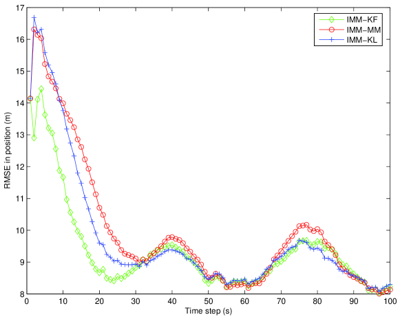
Figure 1: RMSE in position versus time.

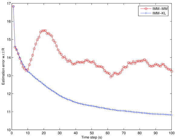
Figure 2: Estimation error of the covariance matrix versus time.

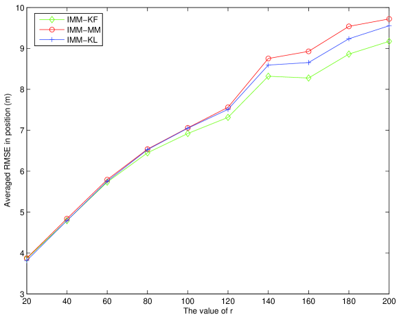
Figure 3: Averaged RMSE in position versus different levels $r$.

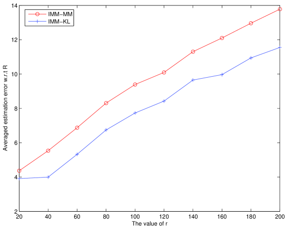
Figure 4: Estimation error of the covariance matrix versus different levels $r$.

V Conclusion

In this paper, we proposed a novel IMM estimation approach with random matrices. Instead of using the moment matching method to address of the combination of a set of weighted inverse-Wishart distributions in the IMM estimation, the weighted Kullback-Leibler divergence is applied and a closed form solution can be derived. Simulation results show that the proposed filter outperforms the previous work using the moment matching method. The proposed approach can be expected to be used for maneuvering extended targets tracking where the target extent is modeled via a random matrix [27, 28, 32, 29, 30, 31].

References

- [1] Costa, O.L.V., Fragoso, M.D., Marques, R.P., Discrete-Time Markov Jump Linear Systems. New York: Springer, 2005.
- [2] Y. Bar-Shalom, X.R. Li, T. Kirubarajan, Estimation with Applications to Tracking and Navigation, Wiley-Interscience, 2001.
- [3] Y. Zhang, X.R. Li, “Detection and diagnosis of sensor and actuator failures using IMM estimator”, IEEE Trans. Aerosp. Electron. Syst., vol. 34, no. 4, pp. 1293-1313, 1998.
- [4] J. Moore, V. Krishnamurthy, “De-interleaving pulse trains using discrete-time stochastic dynamic-linear models”, IEEE Trans. Signal Process., vol. 42, no. 11, pp. 3092-3103, 1994.
- [5] G.A. Ackerson, K.S. Fu, “On state estimation in switching environments”, IEEE Trans. Automat. Contr., vol. 15, no. 1, pp. 10-17, 1970.
- [6] Blom, H., Bar-Shalom, Y., “The interacting multiple model algorithm for systems with Markovian switching coefficients”, IEEE Transactions on Automatic Control, vol. 33, no. 8, pp. 780-783, 1988.
- [7] S. McGinnity, G. Irwin, “Multiple model bootstrap filter for maneuvering target tracking”, IEEE Trans. Aerosp. Electron. Syst., vol. 36, no. 3, pp. 1006-1012, 2000.
- [8] Doucet, A., Gordon, N.J., Krishnamurthy, V., “Particle filters for state estimation of jump Markov linear systems”, IEEE Transactions on Signal Processing, vol. 49, no. 3, pp. 613-624, 2001.
- [9] Y. Boers, J. Driessen, “Interacting multiple model particle filter”, IEE Proc., Radar Sonar Navig., vol. 150, no. 5, pp. 344-349, 2003.
- [10] Terra, M., Ishihara, J., Jesus G., “Information filtering and array algorithms for discrete-time Markovian jump linear systems”, IEEE Transactions on Automatic Control, vol. 54, no. 1, pp. 158-162, 2009.
- [11] X. R. Li, V. P. Jilkov, “Survey of maneuvering target tracking. Part V: multiple-model methods”, IEEE Trans. Aerosp. Electron. Syst., vol. 41, no. 4, pp. 1255-1321, 2004.
- [12] Zhu, J., Park, J., Lee, K., Spiryagin, M., “Robust extended Kalman filter of discrete-time Markovian jump nonlinear system under uncertain noise”, Journal of Mechanical Science and Technology, vol. 22, no. 6, pp. 1132-1139, 2008.
- [13] Costa, O.L.V., “Linear minimum mean square error estimation for discrete-time Markovian jump linear systems”, IEEE Transactions on Automatic Control, vol. 39, no. 8, pp. 1685-1689, 1994.
- [14] Germani, A., Manes, C., Palumbo, P., “State estimation of stochastic systems with switching measurements: a polynomial approach”, International Journal of Robust and Nonlinear Control, vol. 19, no. 14, pp. 1632-1665, 2009.
- [15] Germani A., Manes, C., Palumbo, P., “Filtering for bimodal systems: the case of unknown switching statistics”, IEEE Transactions on Circuits and Systems I: Regular Papers, vol. 53, no. 6, pp. 1266-1277, 2006.
- [16] Li, W., Jia, Y., “Distributed interacting multiple model filtering fusion for multiplatform maneuvering target tracking in clutter”, Signal Processing, vol. 90, no. 5, pp. 1655-1668, 2010.
- [17] Srkk, S., Nummenmaa, A., “Recursive noise adaptive Kalman filtering by variational Bayesian approximations”, IEEE Transactions on Automatic Control, vol. 54, no. 3, pp. 596-600, 2009.
- [18] Gao, X., Chen, J., Tao, D., Li X., “Multi-sensor centralized fusion without measurement noise covariance by variational Bayesian approximation”, IEEE Transactions on Aerospace and Electronic Systems, vol. 47, no. 1, pp. 718-727, 2011.
- [19] Li, W., Jia Y., “State estimation for jump Markov linear systems by variational Bayesian approximation”, IET Control Theory and Applications, vol. 6, no. 2, pp. 319-326, 2012.
- [20] Gupta, A.K., Nagar, D.K., Matrix Variate Distributions, London: Chapman and Hall, 1999.
- [21] Li, W., Jia Y., “Adaptive filtering for jump Markov systems with unknown noise covariance”, IET Control Theory and Applications, vol. 7, no. 13, pp. 1765-1772, 2013.
- [22] C. M. Bishop, Pattern Recognition and Machine Learning, Springer, 2006.
- [23] S. M. Ali, S. D. Silvey. “A general class of coefficients of divergence of one distribution from another”, J. Roy. Stat. Soc., vol. 28, no. 1, pp. 131-142, 1966.
- [24] G. Battistelli, L. Chisci, “Kullback-Leibler average, consensus on probability densities, and distributed state estimation with guaranteed stability”, Automatica, vol. 50, no. 3, pp. 707-718, 2014.
- [25] H. Akaike, “Information theory and an extension of the maximum likelihood principle”, Proceedings of the Second International Symposium on Information Theory, pp. 267-281, 1973.
- [26] Orguner, U., A variational measurement update for extended target tracking with random matrices, IEEE Transactions on Signal Processing, vol. 60, no. 7, pp. 3827-3834, 2012.
- [27] Koch, W., “Bayesian approach to extended object and cluster tracking using random matrices”, IEEE Transactions on Aerospace and Electronic Systems, vol. 44, no. 3, pp. 1042-1059, 2008.
- [28] Feldmann, M., Franken, D., Koch, W., “Tracking of extended objects and group targets using random matrices”, IEEE Transactions on Signal Processing, vol. 59, no. 4, pp. 1409-1420, 2011.
- [29] Lan, J., Li, X.R., “Tracking of extended object or target group using random matrix, part I: New model and approach”, In Proceedings of the International Conference on Information Fusion, Singapore, July 2012, pp. 2177-2184.
- [30] Lan, J., Li, X.R., “Tracking of extended object or target group using random matrix, part II: Irregular object”, In Proceedings of the International Conference on Information Fusion, Singapore, July 2012, pp. 2185-2192.
- [31] Lan, J., Li, X.R., “Tracking of maneuvering non-ellipsoidal extended object or target group using random matrix”, IEEE Transactions on Signal Processing, vol. 62, no. 9, pp. 2450-2463, 2014.
- [32] K. Granstrom, U.” Orguner, “New prediction for extended targets with random matrices, IEEE Transactions on Aerospace and Electronic Systems, vol. 50, no. 2, pp. 1577-1589, 2014.