Equation of State for QCD at finite temperature and density. Resummation versus lattice data
Abstract
The perturbative series for finite-temperature field theories has very poor convergence properties and one needs a way to reorganize it. In this talk, I review two ways of reorganizing the perturbative series for field theories at finite temperature and chemical potential, namely hard-thermal-loop perturbation theory (HTLpt) and dimensional reduction (DR). I will present results for the pressure, trace anomaly, speed of sound and the quark susceptibilities from a 3-loop HTLpt calculation and for the quark susceptibilities using DR at four loops. A careful comparison with available lattice data shows good agreement for a number of physical quantities.
Keywords:
QCD equation of state, Quark-gluon plasma, Hard-thermal-loop perturbation theory, Lattice QCD calculations.:
64.30.Ef, 12.38.Mh, 12.38.Gc.1 Introduction
In this talk I would like to discuss a problem that has been around for a couple of decades namely the poor convergence of the perturbative series of the thermodynamic functions of hot and dense QCD. The weak-coupling expansion of the QCD pressure has a very long story going back to the late 1970s shuryak ; chin ; kapusta79 ; toimela ; arnoldzhai1 ; arnoldzhai2 ; zhaikastening ; eric3 and the interest has in part been spurred by application to quark-gluon plasma phenomenology in heavy-ion collisions. The calculational frontier has been pushed to order at zero chemical potential kajantie and finite chemical potential aleksi0 ; aleksi ; ibb .
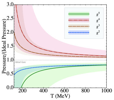
In Fig. 1, we show the weak-coupling expansion of the
QCD pressure with normalized to that of an ideal gas of
quarks and gluons
through order , , , and .
The curves are obtained by using the strong coupling constant
evaluated at the renormalization scale .
The bands are obtained by varying the renormalization scale by a factor of two
around this central value.
As successive terms in the weak-coupling expansion are added,
the predictions for the pressure fluctuate wildly and the
sensitivity to the renormalization scale grows.
Due to asymptotic freedom, the weak-coupling expansion does converge
for sufficiently high temperatures.
However, this is only the case for temperatures many orders of magnitude
larger than the critical temperature for deconfinement.
For example the order- term is smaller than
the order- only if is larger than approximately .
We note in passing that the poor convergence is not specific to QCD,
it is a generic feature of hot quantum field theories.
This together with the large corrections suggests that the
problem is in the soft sector of the theory, i.e. momenta on the order
of , and is not related to the breakdown of perturbation theory
due to infrared divergences at four loops (Linde’s problem) linde .
There are several ways of reorganizing the perturbative
series review1 ; review2 , here I will focus on
hard-thermal-loop perturbation theory (HTLpt) and dimensional
reduction (DR).
The results presented in this talk are published
in the papers leg1 ; syl ; 3l1 ; 3l2 .
2 Reorganization of the perturbative series
2.1 Screened perturbation theory
Before we discuss hard-thermal-loop perturbation theory in some detail, it is useful to take a step back and discuss resummation in a self-interacting scalar field theory. The starting point is the Euclidean Lagrangian for massless -theory
| (1) |
We are interested in calculating perturbative corrections to various
quantities, for example the two-point function.
Fig. 2 shows diagrammatically the inverse propagator to one-loop
order.

Calculating the one-loop diagram, the inverse propagator can be written as
| (2) |
where . For hard momenta, i.e. for or , we see that the correction is a perturbative correction at weak coupling. However, for soft momenta, i.e. for or , the correction is as large as the tree-level term. This is the simplest example of a hard thermal loop (HTL) eric , namely a loop correction which is dominated by hard loop momenta on the order and is as large as a tree-level term. In this case, the HTL is a simple local mass term. The fact that this term is as large as the tree-level term suggests that we need to reorganize perturbation theory at high temperature.
Screened perturbation theory (SPT) spt0 ; chiku ; spt3 ; spt4 ; spt5 is one way of reorganizing the perturbative series, which was inspired by variational perturbation theory vpt1 ; vpt2 ; vpt3 . It is defined by writing the Lagrangian as follows
| (3) | |||||
| (4) |
The perturbative expansion is then an expansion around an ideal gas of
massive particles. In other words, we incorporate a (thermal)
mass to all loop orders via the propagator.
In order to avoid overcounting of Feynman diagrams, we
need to subtract the quadratic term and consider it as an interaction
on the same footing as the quartic interaction. The Feynman rules
for SPT are shown in Fig. 3

Using a massive propagator, all infrared divergences are screened and one can, in principle, calculate Feynman diagrams at any order in screened perturbation theory. However, at this stage the mass parameter in the Lagrangian is arbitrary and in order to complete a calculation in SPT, we need a prescription for it. I will return to this point later in my talk.
2.2 Hard-thermal-loop perturbation theory
Hard-thermal-loop perturbation theory is a generalization of SPT to gauge theories and was developed by Andersen, Braaten, and Strickland over a decade ago andersen1 . In gauge theories one cannot simply add and subtract a local mass term for the gluons as this would violate gauge invariance.
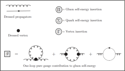
Looking more carefully at the gluon self-energy function at one-loop order, one realizes that there are contributions (see Fig. 4) which are as large as the tree-level term for soft external momenta. The corresponding loop integral is again dominated by hard momenta and is another example of a hard thermal loop.

The contribution to the self-energy function
from the one-loop diagram is then used
to construct an effective two-point function, as shown in Fig. 5.

It turns out that not only the two-point function receives loop
corrections that are as a large as the tree-level contribution, but
also higher -point functions do. Thus, we need to use
effective vertices together with effective propagators, see Fig. 6.
This is essential in order to maintain gauge invariance.

There is a nonlocal effective action that generated all the hard-thermal-loop -point functions wong ; efflag1 . It can be written in a manifestly gauge invariant form and reads
| (5) |
where is the field strength, is the covariant derivative, and and are the Debye screening mass and fermion mass parameters. Moreover, is lightlike four-vector with being a unit three-vector. The bracket indicates an angular average over the directions of . The QCD Lagrangian is then reorganized by writing
| (6) |
where the QCD Lagrangian in Minkowski space is
| (7) |
The term contains counterterms necessary to cancel the ultraviolet divergences in perturbative calculations, and contains the counterterms necessary to cancel additional ultraviolet divergences generated by HTLpt. is the ghost term that depends on the gauge-fixing term , however we emphasize that HTLpt is a gauge invariant framework by construction. It can be used to calculate both static and dynamical quantities. We point out, however, that HTLpt suffers from the same infrared problems related to the magnetic mass as does perturbative QCD, cf. Linde’s problem nan . HTLpt systematically shifts the perturbative expansion from being around an ideal gas of massless particles to being around a gas of massive quasiparticles which are the appropriate physical degrees of freedom at high temperature and/or chemical potential.
Note that the HTLpt Lagrangian (6) reduces to the QCD Lagrangian (7) if we set . The parameter is an expansion parameter and HTLpt is defined by an expansion in powers of around . For example at leading order in , , HTLpt describes free massive quasiparticles that include screening effects and Landau damping. At higher orders in , we include interactions among these quasiparticles.
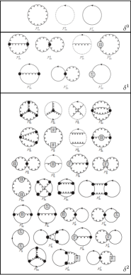
In Fig. 7 we show the diagrams contributing
to the pressure at order
, , and (left).
The different insertions are
shown to the right.
A three-loop calculation at finite temperature and with a separate quark chemical potential for each quark yields 3l1 ; 3l2 .
| (8) | |||||
where the sums over and include all quark flavors, , is the pure-glue contribution 3loopglue2 , , etc, and . Moreover , where is the digamma function and where . , , , with . Note that there are two renormalization scales and , we use former in the purely gluonic graphs and the latter in all other graphs. In this way the susceptibilities vanish in the limit . In addition, the thermodynamic potential produces the correct weak-coupling result if expanded in a strict power series in .
2.3 Dimensional reduction
In scalar field theory, we have seen that the resummed effective propagator
is of the form , where is on the order .
There are two momentum scales in scalar theory (and in QED), namely the
hard scale and the soft scale (, where is the electric charge).
At weak coupling, the term is a perturbative correction
to the propagator for the nonzero Matsubara modes, while it is essential
to include for the static mode . At weak coupling, one therefore
has to well separated mass scales and one can integrate out the
nonzero Matsubara frequencies to obtain an effectice
three-dimensional field theory for the zeroth Matsubara
mode eric2 ; laine . The idea is shown in Fig. 8, where
the imaginary time dimension is and so the system becomes effectively
three-dimensional at high temperature.

The scale can be integrated out perturbatively and in the case of scalar -theory, the effective three-dimensional Lagrangian becomes
| (9) |
where contains higher-order operators. The parameters of the effective Lagrangian are functions of , , and a renormalization scale . For example and to leading order in . In QED, dimensional reduction can be carried out the same way and one obtains an effective three-dimensional theory for a massive scalar field , which can be identified with the zeroth component of the original gauge field, and a gauge field , which can identified with the spatial components of the original gauge field 222The fermions are massive since so they are integrated out as well.. In QCD, it is somewhat more complicated as we have three momentum scales, namely the hard scale , soft scale , and the supersoft scale . At weak coupling, we then have three well separated momentum scales and we can successive integrate out the scales and . Integrating out the scale , we obtain an effective three-dimensional theory, Electrostatic QCD (EQCD), whose Lagrangian is
| (10) |
where is the nonabelian field strength tensor and is a scalar field in the adjoint representation of the gauge group . Moreover, is the color electric screening mass, is the scalar self-coupling, and dimred . The term contains all higher-order operators that start to contribute to the pressure beyond order . We note in passing that EQCD breaks the center symmetry of four-dimensinonal QCD, which can be remedied by formulating the theory in terms of Wilson loop type variables instead of the field poly1 ; poly2 . However, for high temperatures, this is of little consequence as the probability of thermal fluctuations crossing the barriers that separate the trivial minimum we are expanding about, and other minima is exponentially small.
Dimensional reduction has been carried out both at zero density finns1 ; finns2 as well as at finite density aleksi to order . The color electric screening mass is on the order , and as a result, we integrate it out perturbatively to obtain a second effective field theory (Magnetostatic QCD). This theory is plagued with infrared divergences in perturbation theory and must be treated nonperturbatively using lattice simulations. We can now write the pressure in QCD as a sum of contributions from the different momentum scales
| (11) |
The contribution from the hard scale comes from dimensional reduction (which can be identified with the unit operator in ). The contribution from the soft scale comes from calculations in using EQCD, while the contribution from the supersoft scale comes from calculations in MQCD. However, MQCD contributes first at order , and as a result, we can ignore these contributions if we restrict ourselves to order .
3 Numerical results
We next present our numerical results. Physical quantities such as the pressure and susceptibilities depend on the mass parameters and as well as the running coupling and the renormalization scales and We fixed the scale by requiring that , which is obtained from lattice measurements runbaza . Using one-loop running this gives MeV, while two-loop running gives MeV. We used one-loop running for HTLpt and two-loop running for DR. We take the central values and in our HTL calculations. In our DR calculations, we used a central value of for , which is based on the principle of fastest apparent convergence. This can be generalized to nonzero density, see Ref. syl for details. In all plots, the thick lines indicate the results obtained using these central values and the bands are obtained by varying the scales by a factor of two. For the numerical results presented in this talk, we use and .
As mentioned before, one needs to give a prescription for the mass parameters and . One can think of a variational prescription such as
| (12) |
where is the free energy. At one-loop order in HTLpt, the only solution is the trivial solution. At higher orders, this equation has complex solution for some values of the coupling. We therefore decided to use value for the fermion mass parameter and the Debye mass given by the two-loop expression for the mass parameter in EQCD aleksi ,
| (13) | |||||
When we evaluate various physical quantities either in HTLpt or DR, it is essential that we do not expand the mass parameter in powers of , but keep the full -dependence to resum the perturbative series.
3.1 Pressure
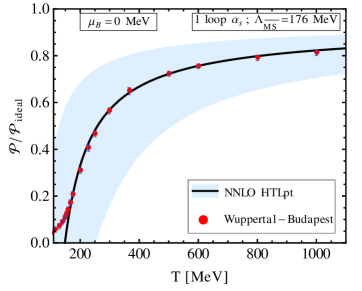
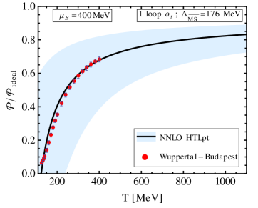
In Fig. 9, we show the normalized pressure as a function of
for (left) and MeV (right).
The solid lines are obtained by using the
central value
and
for the renormalization scales. The blue bands
are obtained by varying this scale around the central value by a factor
of two. The lattice data are from the Budapest-Wuppertal
collaboration borsap ; borsapmu . The agreement with the
central line and the lattice data is remarkable all the way down
to approximately MeV. Since HTLpt is a perturbative approach that
does not incorporate the center symmetry, there is no
reason to expect agreement with the data at temperatures close to
and the agreement seen may be fortuitous.
3.2 Susceptibilities
We next turn to the quark and baryon susceptibilities. The pressure is a function of the temperature and the quark chemical potentials . Furthermore, we can expand the pressure as a Taylor series in powers of around zero chemical potential:
| (14) |
where the coefficients are given by
| (15) |
Below, we will use the shorthand notation for the susceptibilities by specifying derivatives by a string of quark flavors in superscript form, e.g. , , etc. We will also interested in the baryon-number susceptibilities, which are defined by
| (16) |
Using the relation and the chain rule we can find relations between the quark and baryon susceptibilities. For example, one finds
| (17) |
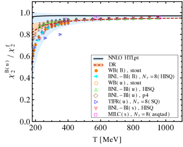
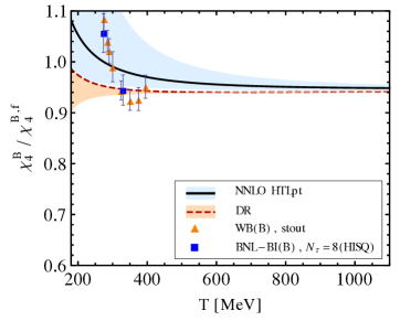
In Fig. 10, we compare the scaled second (left) and fourth-order (right) baryon number susceptibility from HTLpt and DR compared with various lattice data. Both resummation schemes are in good agreement with the data. We also notice that the band using DR is significantly smaller than that obtained in HTLpt.
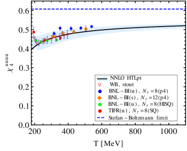
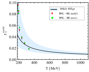
In Fig. 11, we show the NNLO HTLpt fourth order diagonal single quark number susceptibility (left) and the only non-vanishing fourth order off-diagonal quark number susceptibility (right) with lattice data. Again the agreement between the HTLpt prediction and the lattice data is good.
3.3 Interaction measure and speed of sound
The interaction measure is given by
| (18) |
where is the energy density.
Since this quantity is the trace of the energy-momentum tensor
and vanishes for an ideal gas of massless particles,
it is also referred to as the trace anomaly.
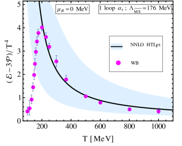
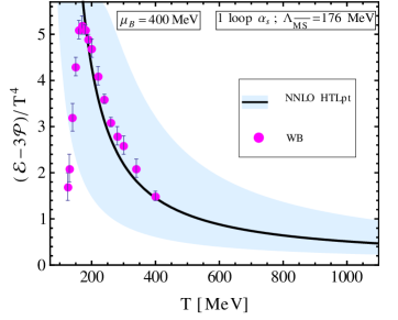
In Fig. 12, we show the interaction measure
normalized by as a function of temperature for
(upper left panel) and
MeV (upper right panel).
The lattice data are from the Wuppertal-Budapest
collaboration borsap ; borsapmu .
We see that the agreeement between the prediction from HTLpt
and lattice data is very good all the way down to MeV, which
is very near where the peak is located. For lower values of the temperature,
HTLpt fails completely, but this is not very surprising.
There is no reason to expect that resummed perturbation theory
works close to the QCD transition temperature.
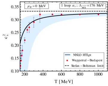
Another quantity which is phenomenologically interesting is the speed of sound. The speed of sound squared is defined as
| (19) |
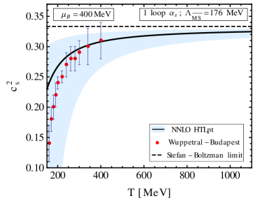
In Fig. 13 we plot the NNLO HTLpt speed of sound squared for (left) and MeV (right) together with lattice data from Refs. borsap and borsapmu . As we can see from this figure, there is quite good agreement between the NNLO HTLpt speed of sound and the lattice data when the central value of the scale is used.
4 Summary and Outlook
In this talk, I have presented results for QCD thermodynamic functions using hard-thermal-loop perturbation theory and dimensional reduction. We note that our results are completely analytic and that, after we have chosen the renormalization scales and , there are no fit parameters. Comparing our results with available lattice data, they suggest that for temperatures above MeV (depending on the quantity we are looking at), the pressure, quark number susceptibilities, and other quantities can be accurately described via resummed perturbation theory.
Hard-thermal-loop perturbation theory represents a gauge-invariant reorganization of the perturbative series. It is formulated in Minkowski space and so can be used to calculate static and dynamical quantities alike. The good agreement between HTLpt and lattice offers some hope that applications to real-time quantities will be useful.
There are several directions for future work. One is to include finite quark masses, another is to resum logarithms to reduce the scale variation of our results. Extending our results to larger values of is also of interest as there currently no other first principle method is available.
References
- (1) E. V. Shuryak, Sov. Phys. JETP 47, 212–219 (1978).
- (2) S. A. Chin, Phys. Lett. B 78, 552–555 (1978).
- (3) J. I. Kapusta, Nucl. Phys. B 148, 461–498 (1979).
- (4) T. Toimela, Phys. Lett. B 124, 407–409 (1983).
- (5) P. Arnold, C. X. Zhai, Phys. Rev. D 50, 7603–7623 (1994).
- (6) P. Arnold, C. X. Zhai, Phys. Rev. D 51, 1906–1918 (1995).
- (7) C. X. Zhai and B. M. Kastening, Phys. Rev. D 52, 7232–7246 (1995).
- (8) E. Braaten, and A. Nieto, Phys. Rev. D 53, 3421–3437 (1996).
- (9) K. Kajantie, M. Laine, K. Rummukainen and Y. Schröder, Phys. Rev. D 67, 105008 (2003).
- (10) A. Vuorinen, Phys. Rev. D 67, 074032 (2003).
- (11) A. Vuorinen, Phys. Rev. D 68, 054017 (2003).
- (12) A. Ipp, K. Kajantie, A. Rebhan, and A. Vuorinen, Phys. Rev. D 74, 045016 (2006).
- (13) A. D. Linde, Phys. Lett. B 96, 289–292 (1980).
- (14) J. O. Andersen and M. Strickland, Ann. Phys. 317, 281–353 (2005).
- (15) U. Kraemmer and A. Rebhan, Rept. Prog. Phys. 67, 351–431 (2004).
- (16) J. O. Andersen, L. E. Leganger, M. Strickland, and N. Su, JHEP 08, 053 (2011).
- (17) S. Mogliacci, J. O. Andersen, M. Strickland, N. Su, and A. Vuorinen, JHEP 12, 055 (2013).
- (18) N. Haque, J. O. Andersen, M. G. Mustafa, M. Strickland, and N. Su, Phys. Rev. D 89, 061701 (2014).
- (19) N. Haque, A. Bandyopadhyay, J. O. Andersen, M. G. Mustafa, M. Strickland, and N. Su, JHEP 05, 027 (2014).
- (20) E. Braaten, and R. D. Pisarski, Nucl. Phys. B, 337, 569–634 (1990).
- (21) F. Karsch, A. Patkos and P. Petreczky, Phys. Lett. B 401, 69–73, (1997).
- (22) S. Chiku and T. Hatsuda, Phys. Rev. D 58, 076001 (1998).
- (23) J. O. Andersen, E. Braaten and M. Strickland, Phys. Rev. D 63, 105008 (2001).
- (24) J. O. Andersen and L. Kyllingstad, Phys. Rev. D 78, 076008 (2008).
- (25) J. O. Andersen and M. Strickland, Phys. Rev. D 64, 105012 (2001) .
- (26) V. I. Yukalov, Teor. Mat. Fiz. 26, 403–413, (1976).
- (27) P. M. Stevenson, Phys. Rev. D 23, 2916–2944 (1981).
- (28) A. Duncan and M. Moshe, Phys. Lett. B 215, 352–358 (1988).
- (29) J. O. Andersen, E. Braaten, and M. Strickland, Phys. Rev. Lett. 83, 2139–2142 (1999).
- (30) J. C. Taylor, and S. M. H. Wong, Nucl. Phys. B 346, 115–128 (1990).
- (31) E. Braaten, and R. D. Pisarski, Phys. Rev. D 45, 1827–1830 (1992).
- (32) N. Su and K. Tywoniuk, arXiv:1409.3203 [hep-ph].
- (33) J. O. Andersen, M. Strickland, and N. Su, JHEP 1008, 113 (2010).
- (34) E. Braaten, and A. Nieto, Phys. Rev. D, 51, 6990–7006 (1995).
- (35) K. Kajantie, M. Laine, K. Rummukainen, and M. E. Shaposhnikov, Nucl. Phys. B, 458, 90–136 (1996).
- (36) A. Hart, M. Laine, and O. Philipsen, Nucl. Phys. B 586, 443–474 (2000)
- (37) A. Vuorinen and L. G. Yaffe, Phys. Rev. D 74, 025011 (2006).
- (38) P. de Forcrand, A. Kurkela and A. Vuorinen, Phys. Rev. D 77, 125014 (2008).
- (39) K. Kajantie, M. Laine, K. Rummukainen, and Y. Schröder, Phys. Rev. D, 67, 105008 (2003).
- (40) K. Kajantie, M. Laine, K. Rummukainen, and Y. Schröder, JHEP 04, 036 (2003).
- (41) A. Bazavov, N. Brambilla, X. Garcia i Tormo, P. Petreczky, J. Soto, and A. Vairo, Phys. Rev. D 86, 114031 (2012).
- (42) S. Borsányi et al., JHEP 11, 077 (2010).
- (43) S. Borsányi et al., JHEP 08, 53 (2012).
- (44) S. Borsányi, Z. Fodor, S. D. Katz, S. Krieg, C. Ratti, and K. Szabo, JHEP 01 , 138 (2012).
- (45) A. Bazavov et al., Phys. Rev. Lett. 111, 082301 (2013).
- (46) Phys.Rev. D 88, 094021 (2013).
- (47) C. Bernard et al., Phys. Rev. D 71, 034504 (2005).
- (48) S. Datta, R.V. Gavai and S. Gupta, PoS LATTICE2013, 202 (2013).