Physical and cut-off effects of heavy sea quarks

Abstract:

We simulate a theory with two dynamical O($a$) improved Wilson quarks whose mass $M$ ranges from a factor eight up to a factor two below the charm quark mass and at three values of the lattice spacing ranging from 0.066 to 0.034 fm. This theory is a prototype to study the decoupling of heavy quarks. We measure the mass and cut-off dependence of ratios of gluonic observables defined from the Wilson flow or the static potential. The size of the 1/$M$ corrections can be determined and disentangled from the lattice artifacts. The difference with the pure gauge theory is at the percent level when two quarks with a mass of the charm quark are present.

WUP 14-14

DESY 14-209

SFB/CPP-14-86

CERN-PH-TH-2014-215

1 Decoupling of heavy quarks

Heavy quarks are expected to decouple from low energy observables. We consider here only observables where the quarks with mass $M$ contribute through loops and no states with an explicit heavy quark. At energies $E$ much smaller than the mass $M$ of the heavy quark, the theory with $N_{\mathrm{f}}$ quarks, of which one is heavy, is described by an effective Lagrangian with $N_{\mathrm{f}}-1$ quark fields

$${\mathscr{L}}^{(N_{\mathrm{f}}-1)}_{\rm eff}={\mathscr{L}}^{(N_{\mathrm{f}}-1)}_{\rm QCD}(\psi_{\mathrm{light}},\bar{\psi}_{\mathrm{light}},A_{\mu};g_{\mathrm{eff}}(M),m_{\mathrm{light,\,eff}}(M))+{1\over M^{2}}{\mathscr{L}}_{6}\,.$$ (1)

In this sense we denote by $N_{\mathrm{f}}\to N_{\mathrm{f}}-1$ the decoupling of one heavy quark. Here we assume a situation where in finite volume there is a non-anomalous chiral symmetry in the sector of the light quarks (which is spontaneously broken in infinite volume). The terms in the effective Lagrangian have to be gauge-, Euclidean- and chiral-invariant. In particular chiral symmetry forbids a dimension five Pauli term. ${\mathscr{L}}_{6}$ contains composite fields of dimension six. The Pauli term only appears in ${\mathscr{L}}_{6}$ in the combination $m_{\mathrm{light}}\bar{\psi}_{\mathrm{light}}\sigma_{\mu\nu}F_{\mu\nu}\psi_{\mathrm{light}}$ when the light quarks have a mass $m_{\mathrm{light}}$.

At low energies the decoupling of the heavy quark leaves traces through renormalization. The gauge coupling $g_{\mathrm{eff}}(M)$ of the effective theory depends on the mass $M$ of the heavy quark. This dependence comes from the matching of the effective theory with the full theory. When we assume all light quarks to be mass-less and neglect all terms $O(E^{2}/M^{2})$, $g_{\mathrm{eff}}$ is the only coupling in Eq. (1). Only it has to be matched. However, the value of the coupling at a given scale is equivalent to the $\Lambda$-parameter of the theory. This drops out [1] in all dimensionless physical quantities such as ratios

$$R(M)={t_{0}(M)\over w_{0}^{2}(M)}\,,\;{r_{1}(M)\over r_{0}(M)}\,,\;\ldots$$ (2)

Thus for such ratios, the matching is irrelevant. In the same way, the value of the bare improved coupling $\tilde{g}_{0}^{2}$ is irrelevant when one computes ratios such as $r_{1}/r_{0}$ with $r_{1}/a$ and $r_{0}/a$ at the same mass. Therefore these ratios are directly given by their values in the theory with the heavy quark removed up to power corrections in $1/M^{2}$. It is the size of these corrections which we want to estimate here. In the following we denote by $M$ the renormalization group invariant quark mass [2].

$\beta$	$a$ [$\,\mathrm{fm}$]	BC	$T\times L^{3}$	$M/\Lambda_{\rm\overline{MS\kern-0.35002pt}\kern 0.35002pt}$	kMDU
$5.3$	$0.0658(10)$	p	$64\times 32^{3}$	0.638(46)	1
		p	$64\times 32^{3}$	1.308(95)	2
		p	$64\times 32^{3}$	2.60(19)	2
$5.5$	$0.0486($0$7)$	o	$120\times 32^{3}$	0.630(46)	8
		o	$120\times 32^{3}$	1.282(93)	8
		p	$96\times 48^{3}$	2.45(18)	4
$5.7$	$0.0341($0$5)$	o	$192\times 48^{3}$	1.277(94)	4
		o	$192\times 48^{3}$	2.50(18)	8

Table 1: Overview of the ensembles. The entries in the column BC refer to periodic (p) or open (o) boundary conditions. The values of $M/\Lambda=0.63$, $1.28$ and $2.50$ correspond approximately to $M=200$, $400$ and $800$ MeV.

2 Simulations

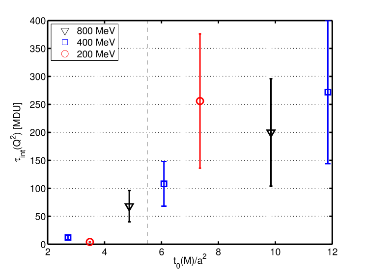
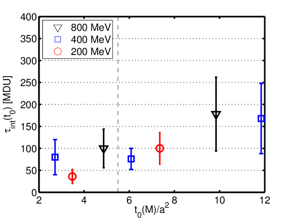
Figure 1: Autocorrelation times of the topological charge squared $Q^{2}$ (left) and of the scale $t_{0}(M)$ (right) as a function of $t_{0}(M)/a^{2}$. Simulations with $t_{0}(M)/a^{2}>5.5$ have been performed with open boundary conditions.

We simulate a model, namely QCD with two heavy, mass-degenerate quarks. The decoupling is then $2\to 0$ and the effective theory, ${\mathscr{L}}^{(N_{\mathrm{f}}-2)}_{\rm eff}$, is the Yang-Mills theory up to $1/M^{2}$ corrections. We use $N_{\mathrm{f}}=2$ O($a$) improved Wilson fermions [3] at three values of the lattice coupling $g_{0}^{2}$ and lattice spacing $a$: $6/g_{0}^{2}=5.3$ ($a=0.0658(10)\,\,\mathrm{fm}$ from [4]), $6/g_{0}^{2}=5.5$ ($a=0.0486(7)\,\,\mathrm{fm}$ from [4]) and $6/g_{0}^{2}=5.7$ ($a=0.0341(5)\,\,\mathrm{fm}$ estimated from the ratio of the scale $t_{0}/a^{2}$ at $6/g_{0}^{2}=5.5$ and $5.7$). Our volumes are such that the lightest pseudo-scalar mass times the box size is $m_{\rm PS}L\geq 7.4$ and $L/r_{0}(M)\geq 3.8$, where significant finite volume effects can be excluded. A list of the simulated ensembles is given in Table 1.

Part of the simulations are performed using periodic boundary conditions (except for anti-periodic boundary conditions in temporal direction for the fermions) and the MP-HMC algorithm [5]. In order to avoid the freezing of the topological charge, for simulations with $t_{0}/a^{2}>5.5$ [6, 7] we adopt open boundary conditions in time and use the publicly available openQCD package [8]. At the smallest lattice spacing $a=0.034\,\,\mathrm{fm}$ we find autocorrelation times for observables such as $t_{0}$ or the topological charge squared of $\tau_{\rm exp}\simeq 250$ MDU (Molecular Dynamics Units), see Fig. 1. Our statistics of $4000$–$8000$ MDU is therefore adequate. The error analysis, based on [9], nevertheless includes the effects of modes with these large autocorrelation times [6]. The cost of our simulations is relatively low compared to simulations in the chiral regime.

The renormalized quark mass $\kern 1.0pt\overline{\kern-1.0ptm\kern-1.0pt}\kern 1.0pt_{{\rm SF}}(L_{1})$ at length scale $L_{1}$ is defined by $\kern 1.0pt\overline{\kern-1.0ptm\kern-1.0pt}\kern 1.0pt_{{\rm SF}}(L_{1})=Z_{\rm A}/Z_{\rm P}(L_{1})\,m$, where the renormalisation factor $Z_{\rm P}(L_{1})$ is defined in the Schrödinger Functional scheme as in [4]. The axial current renormalization factor, $Z_{\rm A}$, is fixed by a chiral Ward identity [10]. For the determination of the PCAC masses we use Tomasz Korzec’s program. The renormalization group invariant mass $M$ is obtained by multiplying $\kern 1.0pt\overline{\kern-1.0ptm\kern-1.0pt}\kern 1.0pt_{{\rm SF}}(L_{1})$ with the factor [11] $M/\kern 1.0pt\overline{\kern-1.0ptm\kern-1.0pt}\kern 1.0pt_{{\rm SF}}(L_{1})=1.308(16)$. The ratio

$$\frac{M}{\Lambda}=\frac{(aM)\,(L_{1}/a)}{(\Lambda L_{1})}$$ (3)

is computed using the values of $L_{1}/a$ from [4] (at $6/g_{0}^{2}=5.7$ we get $L_{1}/a=11.07(17)$) and $\Lambda\,L_{1}$ from [12]. We take the $\Lambda$ parameter to be defined in the ${\rm\overline{MS\kern-0.50003pt}\kern 0.50003pt}$ scheme. The values of $M/\Lambda$ are tabulated in Table 1. Their accuracy is around 7% and is dominated by the relative error of $\Lambda\,L_{1}$.

3 Numerical results

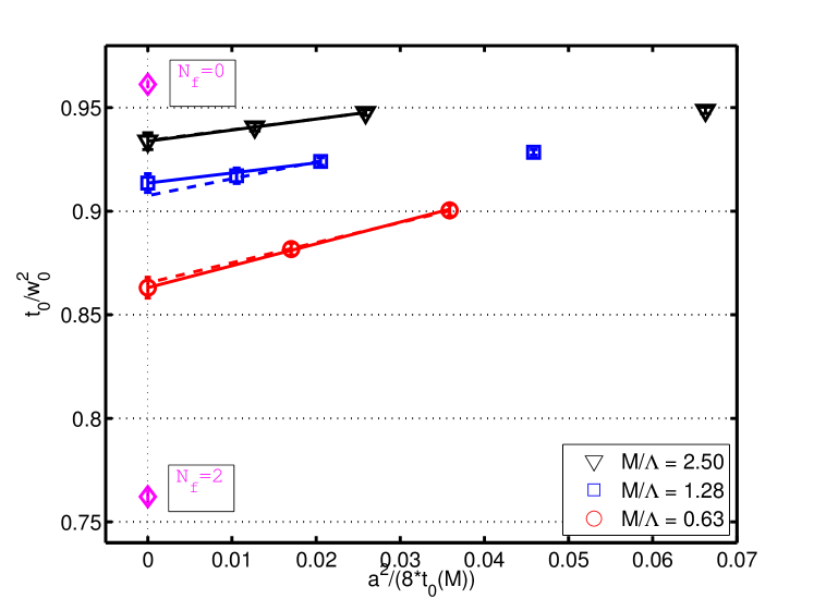
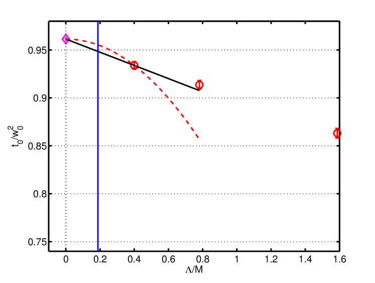
Figure 2: Continuum extrapolation of the ratio $t_{0}/w_{0}^{2}$ (left) and its mass dependence (right).

In order to study the effects of heavy sea quarks, we pick low energy gluonic observables with a strong dependence on the number $N_{\mathrm{f}}$ of sea quarks [13]. For example we consider the scales $t_{0}$ [14] and $w_{0}$ [15] defined from the action density ${\mathcal{E}}(t)=t^{2}\left\langle E(x,t)\right\rangle$, where $t$ is the Wilson flow time, through

$$t_{0} : {\mathcal{E}}(t_{0})=0.3\,,$$ (4)

$$w_{0} : t{\mathcal{E}}^{\prime}(t)|_{t=w_{0}^{2}}=0.3\,.$$ (5)

Furthermore we take the scales $r_{0}$ [16] and $r_{1}$ [17] defined from the static force $F(r)$ through

$$r^{2}F(r)|_{r=r_{c}}=c\,,\quad r_{0}\equiv r_{1.65}\,.$$ (6)

Using these scales we form dimensionless ratios

$$R=t_{0}/w_{0}^{2}\,,\;r_{1}/r_{0}\,,\;r_{0}^{2}/t_{0}\,.$$ (7)

We correct the values of the ratios for small differences in the values of $M/\Lambda$, cf. Table 1. The target values are

$$\frac{M}{\Lambda}=0.63\,,\;1.28\,,\;2.50$$ (8)

and have been chosen to keep the size of the mass corrections small at the finer lattice spacings. The strategy is to fit the data points on the finest lattices linearly in $M/\Lambda$ and in $\Lambda/M$ and then take the slopes from the fits to correct the data at the other lattice spacings. The statistical error of the corrected data is augmented by the difference between the two fits. We neglect in the corrections the error on $M/\Lambda$ since it mainly comes from $\Lambda$ and is therefore common to all points.

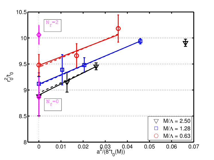
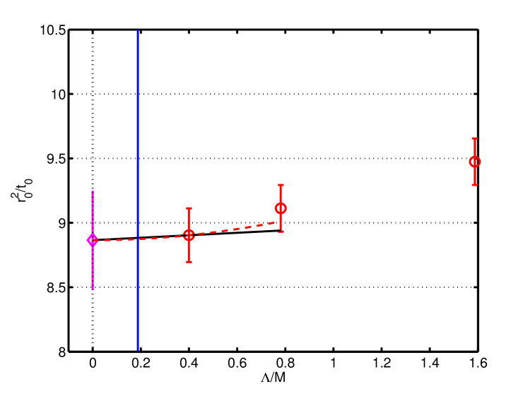
Figure 3: Continuum extrapolation of the ratio $r_{0}^{2}/t_{0}$ (left) and its mass dependence (right).

The continuum extrapolations are done by global fits to the ratios $R_{\rm Lat}$ measured on the lattices, see the left panel of Fig. 2 for $R=t_{0}/w_{0}^{2}$ and of Fig. 3 for $R=r_{0}^{2}/t_{0}$. The continued lines correspond to fits where the slope $s$ of the $a^{2}$ effects at $M=0$ is fixed from [18] ($s\approx 2$ for $R=t_{0}/w_{0}^{2}$, $s\approx 15$ for $R=r_{0}^{2}/t_{0}$)

$$R_{\rm Lat}=R(M)+s\frac{a^{2}}{8t_{0}}\left(1+k_{1}\frac{M}{\Lambda}+k_{2}\frac{M^{2}}{\Lambda^{2}}\right)\,,$$ (9)

where the continuum values $R(M)$ and $k_{1}$, $k_{2}$ are the fit parameters. The dashed lines correspond to fits

$$R_{\rm Lat}=R(M)+k_{0}\frac{a^{2}}{8t_{0}}+k_{1}\frac{a^{2}}{8t_{0}}\frac{M}{\Lambda}$$ (10)

where the continuum values $R(M)$ and $k_{0}$, $k_{1}$ are the fit parameters. The continuum values for $N_{\mathrm{f}}=0$ ($M/\Lambda=\infty$) are taken from [14] and our own results, while the values for $N_{\mathrm{f}}=2$ at $M=0$ are from [13].

	$M/\Lambda$
$R$	$M_{\rm c}/\Lambda$		2.50	1.28	0.63	$0$
	$1/M$-scaled	$1/M^{2}$-scaled
$\sqrt{t_{0}}/w_{0}$	0.34(5)%	0.16(2)%	0.72(11)%	1.26(12)%	2.62(14)%	5.4%
$r_{1}/r_{0}$	0.45(13)%	0.21(6)%	1.0(3)%	1.8(5)%	2.6(6)%	$\approx$4%
$r_{0}/\sqrt{t_{0}}$	0.05(28)%	0.02(12)%	0.1(6)%	0.7(5)%	1.7(5)%	3%

Table 2: Relative effects from decoupling of one heavy sea quark in ratios of quantities of dimension one. At $M_{\rm c}$ we quote the results from interpolations in $1/M$ and $1/M^{2}$.

The continuum extrapolated values are plotted as function of $\Lambda/M$ in the right plots of Fig. 2 and Fig. 3. In order to estimate the size of the mass effects at the charm mass $M_{\rm c}$ (marked by a blue vertical line in the plots), we consider linear (black continued lines) and quadratic (dashed red lines) interpolation between our largest mass $M/\Lambda=2.50$ and the $N_{\mathrm{f}}=0$ ($M/\Lambda=\infty$) values. The relative effects

$${1\over N_{\mathrm{f}}}{R(M)-R(\infty)\over R(\infty)}$$ (11)

are listed in Table 2 for ratios like in Eq. (7) but taken between quantities of dimension one. The factor $1/N_{\mathrm{f}}$ is used to rescale the effects to the case of the decoupling of a single heavy quark $1\to 0$.

4 Conclusions

Our numbers provide an estimate for charm effects in low energy observables in $2+1+1$ simulations. As can be seen from Table 2 these effects are very small, between 1 and 6 permille, in our model of decoupling $2\to 0$ heavy quarks (the numbers in Table 2 are rescaled for decoupling $1\to 0$). This suggests that tiny effects are being missed in $2+1$ simulations at low energies, given that no qualitative difference between decoupling $2\to 0$ and decoupling $2+1+1\to 2+1$ is expected. In this work we investigated low energies up to $r_{1}^{-1}$.

Acknowledgement. We are grateful for computer time allocated for our project on the Konrad and Gottfried computers at the North-German Supercomputing Alliance HLRN, the Cheops computer at the University of Cologne (financed by the Deutsche Forschungsgemeinschaft), the Stromboli cluster at the University of Wuppertal and the PAX cluster at DESY, Zeuthen. This work is supported by the Deutsche Forschungsgemeinschaft in the SFB/TR 09 and the SFB/TR 55.

References

- [1] M. Bruno, J. Finkenrath, F. Knechtli, B. Leder and R. Sommer, On the effects of heavy sea quarks at low energies, arXiv:1410.8374 [hep-lat].
- [2] ALPHA Collaboration, S. Capitani, M. Lüscher, R. Sommer and H. Wittig, Nonperturbative quark mass renormalization in quenched lattice QCD, Nucl. Phys. B 544 (1999) 669 [hep-lat/9810063].
- [3] ALPHA Collaboration, K. Jansen and R. Sommer, O() improvement of lattice QCD with two flavors of Wilson quarks, Nucl. Phys. B 530 (1998) 185 [Erratum-ibid. B 643 (2002) 517] [hep-lat/9803017].
- [4] P. Fritzsch, F. Knechtli, B. Leder, M. Marinkovic, S. Schaefer, R. Sommer and F. Virotta, The strange quark mass and Lambda parameter of two flavor QCD, Nucl. Phys. B 865 (2012) 397 [arXiv:1205.5380].
- [5] M. Marinkovic and S. Schaefer, Comparison of the mass preconditioned HMC and the DD-HMC algorithm for two-flavour QCD, PoS LATTICE 2010 (2010) 031 [arXiv:1011.0911].
- [6] ALPHA Collaboration, S. Schaefer, R. Sommer, and F. Virotta, Critical slowing down and error analysis in lattice QCD simulations, Nucl. Phys. B 845 (2011) 93 [arXiv:1009.5228].
- [7] ALPHA Collaboration, M. Bruno, S. Schaefer, and R. Sommer, Topological susceptibility and the sampling of field space in Nf = 2 lattice QCD simulations, JHEP 1408 (2014) 150 [arXiv:1406.5363].
- [8] M. Lüscher and S. Schaefer, Lattice QCD with open boundary conditions and twisted-mass reweighting, Comput. Phys. Commun. 184 (2013) 519 [arXiv:1206.2809].
- [9] ALPHA Collaboration, U. Wolff, Monte Carlo errors with less errors, Comput. Phys. Commun. 156 (2004) 143 [Erratum-ibid. 176 (2007) 383] [hep-lat/0306017].
- [10] M. Della Morte, R. Sommer, and S. Takeda, On cutoff effects in lattice QCD from short to long distances, Phys. Lett. B 672 (2009) 407 [arXiv:0807.1120].
- [11] ALPHA Collaboration, M. Della Morte, R. Hoffmann, F. Knechtli, J. Rolf, R. Sommer, I. Wetzorke and U. Wolff, Non-perturbative quark mass renormalization in two-flavor QCD, Nucl. Phys. B 729 (2005) 117 [hep-lat/0507035].
- [12] ALPHA Collaboration, M. Della Morte, R. Frezzotti. J. Heitger, J. Rolf, R. Sommer and U. Wolff, Computation of the strong coupling in QCD with two dynamical flavours, Nucl. Phys. B 713 (2005) 378 [hep-lat/0411025].
- [13] M. Bruno and R. Sommer, On the -dependence of gluonic observables, PoS LATTICE2013 (2013) 321 [arXiv:1311.5585].
- [14] M. Lüscher, Properties and uses of the Wilson flow in lattice QCD, JHEP 1008 (2010) 071 [arXiv:1006.4518].
- [15] S. Borsanyi, S. Dürr, Z. Fodor, C. Hoelbling, S. D. Katz, S. Krieg, T. Kurth, L. Lellouch, T. Lippert, C. McNeile and K. K. Szabo, High-precision scale setting in lattice QCD, JHEP 1209 (2012) 010 [arXiv:1203.4469].
- [16] R. Sommer, A new way to set the energy scale in lattice gauge theories and its applications to the static force and in SU(2) Yang-Mills theory, Nucl. Phys. B 411 (1994) 839 [hep-lat/9310022].
- [17] C. W. Bernard, T. Burch, K. Orginos, D. Toussaint, T. A. DeGrand, C. E. DeTar, S. A. Gottlieb, U. M. Heller, J. E. Hetrick and R. L. Sugar, The Static quark potential in three flavor QCD, Phys. Rev. D 62 (2000) 034503 [hep-lat/0002028].
- [18] R. Sommer, Scale setting in lattice QCD, PoS LATTICE2013 (2014) 015 [arXiv:1401.3270].