Non-observable nature of the nuclear shell structure.
Meaning, illustrations and consequences

Abstract

Background

The concept of single-nucleon shells constitutes a basic pillar of our understanding of nuclear structure. Effective single-particle energies (ESPEs) introduced by French and Baranger represent the most appropriate tool to relate many-body observables to a single-nucleon shell structure. As briefly discussed in [T. Duguet, G. Hagen, Phys. Rev. C 85, 034330 (2012)], the dependence of ESPEs on one-nucleon transfer probability matrices makes them purely theoretical quantities that “run” with the non-observable resolution scale $\lambda$ employed in the calculation.

Purpose

Given that ESPEs provide a way to interpret the many-body problem in terms of simpler theoretical ingredients, the goal is to specify the terms, i.e. the exact sense and conditions, in which this interpretation can be conducted meaningfully.

Methods

While the nuclear shell structure is both scale and scheme dependent, the present study focuses on the former. A detailed discussion is provided to illustrate the scale (in)dependence of observables and non-observables and the reasons why ESPEs, i.e. the shell structure, belong to the latter category. State-of-the-art multi-reference in-medium similarity renormalization group and self-consistent Gorkov Green’s function many-body calculations are employed to corroborate the formal analysis. This is done by comparing the behavior of several observables and of non-observable ESPEs (and spectroscopic factors) under (quasi) unitary similarity renormalization group transformations of the Hamiltonian parameterized by the resolution scale $\lambda$.

Results

The formal proofs are confirmed by the results of ab initio many-body calculations in their current stage of implementation. In practice, the unitarity of the similarity transformations is broken due to the omission of induced many-body interactions beyond three-body operators and to the non-exact treatment of the many-body Schrödinger equation. The impact of this breaking is first characterized by quantifying the artificial running of observables over a (necessarily) finite interval of $\lambda$ values. Then, the genuine running of ESPEs is characterized and shown to be convincingly larger than the one of observables (which would be zero in an exact calculation).

Conclusions

The non-observable nature of the nuclear shell structure, i.e. the fact that it constitutes an intrinsically theoretical object with no counterpart in the empirical world, must be recognized and assimilated. Indeed, the shell structure cannot be determined uniquely from experimental data and cannot be talked about in an absolute sense as it depends on the non-observable resolution scale employed in the theoretical calculation. It is only at the price of fixing arbitrarily (but conveniently!) such a scale that one can establish correlations between observables and the shell structure. To some extent, fixing the resolution scale provides ESPEs (and spectroscopic factors) with a quasi-observable character. Eventually, practitioners can refer to nuclear shells and spectroscopic factors in their analyses of nuclear phenomena if, and only if, they use consistent structure and reaction theoretical schemes based on a fixed resolution scale they have agreed on prior to performing their analysis and comparisons.

I Introduction

The concept of single-nucleon shells dates back to the early days of contemporary nuclear physics and constitutes the basic pillar of the nuclear shell model Goeppert-Mayer (1949). In fact, the notion of single-particle energy levels is a fundamental element of a large number of nuclear many-body theories and underlies our understanding of nuclear structure. Based on such a rationale, the correlated shell model has been able to explain the occurrence of extraordinarily stable configurations for specific neutron and proton numbers, known as magic numbers. The universal character of those magic numbers away from the valley of beta stability remains an open question Sorlin and Porquet (2008) currently receiving considerable experimental and theoretical attention, e.g. see Refs. Baumann et al. (2007); Janssens (2009); Wienholtz et al. (2013); Steppenbeck et al. (2013); Otsuka et al. (2010); Holt et al. (2012); Hagen et al. (2012). Whether a certain nucleon number qualifies as a (new) magic number cannot be postulated a priori. Experimentally, several quantities are measured to make such an assessment, e.g., the excitation energy and the collective character of the first $2^{+}$ state, the size of the gap in the one-nucleon addition/removal spectrum, etc. Theoretically, the same quantities need to be computed by solving the many-body Schrödinger equation with sufficient accuracy in order to check whether the picture associated with a magic number holds.

As such, the characterization of the (non-)magic character of a nucleus is based on a set of many-body observables, and does not involve the concept of single-nucleon shells. Still, effective single-particle energies Baranger (1970) (ESPEs) associated with an auxiliary independent-particle-like problem appear as a useful tool to interpret the evolution of many-body observables in terms of simpler theoretical ingredients. The typical picture is that the size of the first $2^{+}$ excitation energy of even-even isotopes as well as the size of the gap between their one-nucleon addition and removal spectra reflect (at least) qualitatively the size of the particle-hole gap in the ESPE spectrum and the value of the associated spectroscopic factors. For instance, a large gap at the Fermi energy in the ESPE spectrum is manifested as a large $2^{+}$ excitation energy with a reduced electric quadrupole transition probability $B(E2)$ to the ground state. Figure 1 illustrates such a correlation for the first $2^{+}$ excitation energy of selected Ca isotopes on the basis of a $pf$ shell-model calculation. The phenomenological GXPF1 Honma et al. (2004) and KB3G Poves et al. (2001) interactions both yield a high $2^{+}$ excitation energy and a large neutron $p_{3/2}-f_{7/2}$ shell gap in ${}^{48}\mathrm{Ca}$, but give very different predictions for the neutron-rich ${}^{54}\mathrm{Ca}$: GXPF1 predicts a large $f_{5/2}-p_{1/2}$ gap and high $2^{+}$ energy, KB3G the opposite.

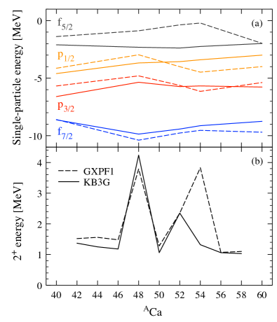
Figure 1: (Color online). Shell-model calculation of selected Ca isotopes performed in the $pf$ valence space with GXPF1 Honma et al. (2004) and KB3G Poves et al. (2001) empirical interactions. Upper panel: effective single-particle energies. Lower panel: first $2^{+}$ excitation energy.

It is thus fair to say that the current paradigm underlining our understanding of nuclear structure provides the single-nucleon shell structure with a certain degree of “reality”. As a matter of fact, reference to an underlying single-particle spectrum is almost systematically made to explain the characteristics and the evolution of low-energy observables in nuclei. Still, such a systematic reference raises basic questions given that individual nucleons do not occupy stationary single-particle states inside a correlated system. This relates to the fact that the only unambiguously defined problem that one can aim at addressing is the interacting many-body problem, which translates into solving the A-body Schrödinger eigenvalue equation

$$H|\Psi^{\text{A}}_{k}\rangle=E^{\text{A}}_{k}|\Psi^{\text{A}}_{k}\rangle\,\,,$$ (1)

and/or its time-dependent counterpart. While the outcome of the former takes the form of A-body energies $E^{\text{A}}_{k}$ and associated A-body states $|\Psi^{\text{A}}_{k}\rangle$, the latter provides reaction cross sections $\sigma(A_{k}\!+\!B_{l}\!\rightarrow\!C_{m}\!+\!D_{n})$ associated with many-body systems transitioning from an initial state $|\Psi^{\text{A+B}}_{\text{initial}}\rangle=|\Psi^{\text{A}}_{k}\rangle\otimes|\Psi^{\text{B}}_{l}\rangle$ to a final state $|\Psi^{\text{C+D}}_{\text{final}}\rangle=|\Psi^{\text{C}}_{m}\rangle\otimes|\Psi^{\text{D}}_{n}\rangle$. As such, single-nucleon shells do not appear explicitly in the formulation of the problem of interest.

The closest accessible quantities relate to the dynamics of a nucleon that is added to or removed from the A-body correlated system, i.e., one-nucleon addition and removal energies $E^{\pm}_{k}\equiv\pm\big{(}E^{\text{A}\pm 1}_{k}-E^{\text{A}}_{0}\big{)}$ along with associated reaction cross sections $\sigma^{\pm}_{k}$. As will be discussed in detail below, the computation of ESPEs, $e^{\text{cent}}_{p}(\lambda)$, combines one-nucleon addition and removal energies $E^{\pm}_{k}$ with associated spectroscopic probability matrices, $\mathbf{S}_{k}^{\pm}(\lambda)$. The dependence of ESPEs on the latter make them intrinsically non-observable quantities that change with the resolution scale $\lambda$ employed in the theoretical description of the system. Thus, a unitary transformation of the Hamiltonian $H(\lambda)\rightarrow H(\lambda^{\prime})$ changes the ESPE spectrum $e^{\text{cent}}_{p}(\lambda)\neq e^{\text{cent}}_{p}(\lambda^{\prime})$ while leaving true observables invariant, e.g. $E^{\pm}_{k}(\lambda)=E^{\pm}_{k}(\lambda^{\prime})$. Expanding on the brief discussion and the limited numerical illustrations provided in Ref. Duguet and Hagen (2012), the goal of the present paper is to further characterize the non-observable character of the nuclear shell structure by presenting a detailed formal analysis along with systematic results obtained from ab initio many-body calculations.

The discussion proposed here is not meant to disqualify the notion of shell structure and the use of ESPEs in our interpretation of experimental data but to specify the terms, i.e., the exact sense and conditions, in which this can be done meaningfully. Still, it is crucial to state upfront that the non-observable character of the shell structure establishes that nuclear shells have no counterpart in the empirical world, i.e. in experiment, and that any apparent correlation between ESPEs and actual observables can only exist in a non-absolute sense. Indeed, ESPEs change with a “parameter” that is internal to the theory and that can be tuned at will without modifying actual observables. As will appear below, this “parameter” presently takes the form of a momentum scale $\lambda$ parameterizing families of unitary transformations that can be arbitrarily applied on the many-body Hilbert space. While these unitary transformations do not modify the physics output, i.e., true observables $O$, they typically change any quantity that results from partitioning these observables, e.g. $O\equiv o_{1}(\lambda)+o_{2}(\lambda)$ or $O\equiv o_{1}(\lambda)\times o_{2}(\lambda)$.

The non-observable nature of the one-nucleon momentum distribution Furnstahl and Hammer (2002), of spectroscopic factors Jennings (2011), or of the one-nucleon shell structure Duguet and Hagen (2012) is not as esoteric or shocking as it may seem at first as it parallels situations encountered in other fields of physics. As a matter of fact, quantum mechanics and quantum field theories possess internal degrees of freedom (e.g. the gauge symmetry) that are essential to their formulation but that are not observable, i.e., nothing in the empirical world can fix their value. Eventually, one can fix this freedom arbitrarily (and conveniently) such that non-observable quantities depending on it acquire a fixed value as well. Still, one must comply with the fact that the behavior of observables cannot be correlated with non-observable quantities in an absolute sense, but only when the internal degree of freedom is fixed to a particular value. Conversely, it is mandatory to agree on the way to fix this freedom prior to doing any comparison or even formulating any discourse on non-observable quantities Furnstahl and Hammer (2002); Duguet and Hagen (2012). The very same care associated with partitioning or factorizing observables is also routine in the discussion of parton distributions in hadronic physics (see, e.g., Sterman et al. (1995)).

The non-observable character of ESPEs make them both resolution scale and theoretical scheme dependent. The present paper focuses on the former by studying at length the“running” of ESPEs with the scale $\lambda$ characterizing similarity renormalization group (SRG) transformations of the Hamiltonian Bogner et al. (2010). Figure 2 anticipates this discussion by illustrating this feature from a microscopic shell model calculation  Holt et al. (2013); Caesar et al. (2013) of ^22,24O. This calculation is performed in a $sd$ valence space and is based on realistic two-nucleon (2N) and three-nucleon (3N) chiral effective field theory ($\chi$-EFT) interactions (see, e.g., Epelbaum et al. (2009); Hammer et al. (2013)) that are evolved to low momenta and further renormalized to the $sd$ shell through third-order many-body perturbation theory Holt et al. (2013). The resolution scale characterizing the 2N interaction is varied from $1.8$ to $2.2$ fm^-1 while keeping the regulator of the 3N interaction unchanged Hebeler et al. (2011); Simonis et al. (2015).

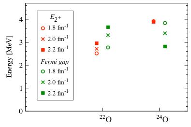
Figure 2: (Color online). Comparison between the Fermi gap in the effective single-particle energy spectrum and the first $2^{+}$ excitation energy in ^22,24O. Results are obtained from a microscopic shell model Holt et al. (2013); Caesar et al. (2013) based on realistic 2N and 3N interactions. Calculations are displayed for three different values of the resolution scale characterizing the 2N interaction; see Ref. Hebeler et al. (2011); Simonis et al. (2015) and the text for details.

In Fig. 2 the resulting values of the Fermi gap in the Baranger ESPE spectrum are compared with the first $2^{+}$ excitation energies. We observe that, while the ESPE Fermi gap typically changes by more than 1 MeV for both nuclei, the $2^{+}$ excitation energy varies by 400 keV in ²²O and only 30 keV in ²⁴O. Moreover, whereas the Fermi gap is relatively close to the 2+ energy for the lowest resolution scale, it can differ by up to 1 MeV for the highest one. Consequently, after varying the resolution scale the correlation between both quantities alluded to in connection with Fig. 1 is weakened, while the observable $2^{+}$ excitation energy is unchanged.

The paper is organized as follows. Section II provides the detailed formal basis for the proper definition of ESPEs and to characterize their non-observable nature. Section III illustrates the formal proofs via state-of-the-art many-body calculations based on $\chi$-EFT 2N and 3N interactions. Conclusions are given in Sec. IV.

II Nuclear shell energies

II.1 Rationale

As already alluded to above, the interest of referring to single-nucleon shells resides in the hypothesis that low-energy observables reflect key patterns of the ESPE spectrum. Besides $2^{+}$ excitation energies, this is supposed to apply first and foremost to one-nucleon separation energies $E^{\pm}_{k}$. Such a rationale translates into the assumption that the observables can be partitioned into a dominant “independent-particle-like” component complemented by many-body correlations, i.e., that one can write schematically

$$\underset{\text{Outcome of Schr. equation}}{\underbrace{E^{\pm}_{k}}}\,\,\,=\,\,\,\underset{\text{Ind. particles}}{\underbrace{e_{p}}}\,\,\,+\,\,\,\underset{\text{Correlations}}{\underbrace{\Delta E_{p\rightarrow k}}}\,.$$ (2)

Equation (2) is a basic tenet of numerous many-body methods. For instance, in many-body perturbation theory, the independent-particle-like contribution refers to a chosen zeroth-order approximation. As such, it is the eigenvalue associated with an ad hoc one-body potential given a priori, e.g., of harmonic-oscillator (HO) or Woods-Saxon type. Alternatively, it can stem from a one-body potential that is derived from an auxiliary condition, e.g., the Hartree-Fock (HF) potential that results from minimizing the correlation contribution to the total binding energy. Another prime example is density functional theory (DFT), where single-particle energies are generated by a local one-body potential that emerges as a result of the constraint that the one-body local density of the Kohn-Sham Slater determinant matches the one of the exact A-body ground-state. Consequently, the single-particle energies typically discussed in the literature reflect a choice (among infinitely many) made by a practitioner. As such, they do not carry any deep meaning, and they certainly do not reflect a unique and unambiguous one-nucleon shell structure of the studied nucleus. Let us now introduce a superior definition of ESPEs Baranger (1970); Duguet and Hagen (2012).

II.2 Definition

The model-independent definition of effective single-particle energies relates them unambiguously to the process of adding (removing) a nucleon to (from) the ground-state of the A-body system of interest in (from) a specific single-particle state. The single-nucleon states in question are not known a priori, but emerge together with ESPEs (see Eq. (11)).

We first specify the second-quantized form of the Hamiltonian entering Eq. (1). It is expressed in an arbitrary single-particle basis as

$$H = T+V^{\text{2N}}+V^{\text{3N}}+\ldots$$ (3b)

$$= \sum_{pq}t_{pq}a^{\dagger}_{p}a_{q}$$

$$+\left(\frac{1}{2!}\right)^{2}\sum_{pqrs}\overline{v}^{\text{2N}}_{pqrs}a^{\dagger}_{p}a^{\dagger}_{q}a_{s}a_{r}$$

$$+\left(\frac{1}{3!}\right)^{2}\sum_{pqrstu}\overline{v}^{\text{3N}}_{pqrstu}a^{\dagger}_{p}a^{\dagger}_{q}a^{\dagger}_{r}a_{u}a_{t}a_{s}$$

$$+\ldots\,,$$

where $\overline{v}^{\text{2N}}_{pqrs}$ and $\overline{v}^{\text{3N}}_{pqrstu}$ denote antisymmetrized matrix elements of 2N and 3N interactions while dots symbolize omitted higher-body forces.

Next, we introduce the probability amplitudes $\mathbf{U}_{\mu}$ ($\mathbf{V}_{\nu}$) to reach a specific eigenstate $|\Psi^{\text{A+1}}_{\mu}\rangle$ ($|\Psi^{\text{A-1}}_{\nu}\rangle$) of the A+1 (A-1) system by adding (removing) a nucleon in (from) a single-particle state to (from) the ground state $|\Psi^{\text{A}}_{0}\rangle$ of an even-even system. Those amplitudes characterize direct one-nucleon addition and removal processes and can be expanded in an arbitrary, e.g., spherical, single-particle basis $\{a^{\dagger}_{p}\}$ according to

$$U^{p}_{\mu} \equiv \langle\Psi^{\text{A}}_{0}|a_{p}|\Psi^{\text{A+1}}_{\mu}\rangle\,,$$ (4a)

$$V^{p}_{\nu} \equiv \langle\Psi^{\text{A}}_{0}|a^{\dagger}_{p}|\Psi^{\text{A-1}}_{\nu}\rangle\,.$$ (4b)

From these amplitudes, one builds spectroscopic probability matrices for the nucleon addition and removal, $\mathbf{S}_{\mu}^{+}\equiv\mathbf{U}_{\mu}\mathbf{U}^{\dagger}_{\mu}$ and $\mathbf{S}_{\nu}^{-}\equiv\mathbf{V}^{\ast}_{\nu}\mathbf{V}^{T}_{\nu}$, respectively. Their elements are

$$S_{\mu}^{+pq} \equiv \langle\Psi^{\text{A}}_{0}|a_{p}|\Psi^{\text{A+1}}_{\mu}\rangle\langle\Psi^{\text{A+1}}_{\mu}|a^{\dagger}_{q}|\Psi^{\text{A}}_{0}\rangle\,\,\,,$$ (5a)

$$S_{\nu}^{-pq} \equiv \langle\Psi^{\text{A}}_{0}|a^{\dagger}_{q}|\Psi^{\text{A-1}}_{\nu}\rangle\langle\Psi^{\text{A-1}}_{\nu}|a_{p}|\Psi^{\text{A}}_{0}\rangle\,\,\,.$$ (5b)

Tracing the latter matrices over the one-body Hilbert space ${\cal H}_{1}$ provides spectroscopic factors

$$SF_{\mu}^{+} \equiv \text{Tr}_{{\cal H}_{1}}\!\left[\mathbf{S}_{\mu}^{+}\right]=\sum_{p\in{\cal H}_{1}}\left|U^{p}_{\mu}\right|^{2}\,\,,$$ (6a)

$$SF_{\nu}^{-} \equiv \text{Tr}_{{\cal H}_{1}}\!\left[\mathbf{S}_{\nu}^{-}\right]=\sum_{p\in{\cal H}_{1}}\left|V^{p}_{\nu}\right|^{2}\,\,,$$ (6b)

which are nothing but the norms of the spectroscopic amplitudes. A spectroscopic factor sums the probabilities that an eigenstate of the A+1 (A-1) system can be described as a nucleon added to (removed from) a single-particle state on top of the ground state of the A-nucleon system.

One can then gather the complete spectroscopic information associated with one-nucleon addition and removal processes into the so-called spectral function $\mathbf{S}(\omega)$. The spectral function denotes an energy-dependent matrix defined on ${\cal H}_{1}$ through

$$\mathbf{S}(\omega) \equiv \!\!\!\!\!\sum_{\mu\in{\cal H}_{A\!+\!1}}\!\!\!\mathbf{S}_{\mu}^{+}\,\,\delta(\omega-E_{\mu}^{+})+\!\!\!\!\!\sum_{\nu\in{\cal H}_{A\!-\!1}}\!\!\!\mathbf{S}_{\nu}^{-}\,\,\delta(\omega-E_{\nu}^{-}),$$

where the first (second) sum is restricted to eigenstates of $H$ in the Hilbert space ${\cal H}_{A\!+\!1}$ (${\cal H}_{A\!-\!1}$) associated with the A+1 (A-1) system. Note that $\mathbf{S}(\omega)$ is directly related to the imaginary part of Dyson’s one-body Green’s function $\mathbf{G}(\omega)$ Dickhoff and Barbieri (2004). Taking the trace of $\mathbf{S}(\omega)$ provides the spectral strength distribution (SDD)

$${\cal S}(\omega) \equiv \text{Tr}_{{\cal H}_{1}}\!\left[\mathbf{S}(\omega)\right]$$

$$= \!\!\!\!\!\sum_{\mu\in{\cal H}_{A\!+\!1}}\!\!\!\!SF_{\mu}^{+}\,\delta(\omega-E_{\mu}^{+})+\sum_{\nu\in{\cal H}_{A\!-\!1}}\!\!\!\!SF_{\nu}^{-}\,\delta(\omega-E_{\nu}^{-})\,,$$

which is a basis-independent function of the energy.

We also introduce the $n^{\text{th}}$ moment of the spectral function

$$\mathbf{M}^{(n)}\equiv\int_{-\infty}^{+\infty}\omega^{n}\,\mathbf{S}(\omega)\,d\omega,$$ (8)

which defines an energy-independent matrix on ${\cal H}_{1}$. Using the anti-commutation rule of creation and annihilation operators $\{a_{p},a^{\dagger}_{q}\}=\delta_{pq}$, the zero moment is shown to be nothing but the identity matrix

$$\mathbf{M}^{(0)}=\sum_{\mu\in{\cal H}_{A\!+\!1}}\mathbf{S}_{\mu}^{+}+\sum_{\nu\in{\cal H}_{A\!-\!1}}\mathbf{S}_{\nu}^{-}=\mathbf{1}\,.$$ (9)

This sum rule provides each diagonal matrix element of $\mathbf{S}(\omega)$ with the meaning of a probability distribution function (PDF) in the statistical sense, i.e., the combined probability of adding a nucleon to or removing a nucleon from a specific single-particle basis state $|p\rangle$ integrates to 1 when summing over all the final states of the A$\pm$1 systems.

The first moment $\mathbf{M}^{(1)}$ of the spectral function defines the so-called centroid matrix

$$\mathbf{h}^{\text{cent}} \equiv \sum_{\mu\in{\cal H}_{A\!+\!1}}\mathbf{S}_{\mu}^{+}E_{\mu}^{+}+\sum_{\nu\in{\cal H}_{A\!-\!1}}\mathbf{S}_{\nu}^{-}E_{\nu}^{-}\,\,\,.$$ (10)

Effective single-particle energies are nothing but the eigenvalues $\{e^{\text{cent}}_{p}\}$ of the centroid field French (1966); Baranger (1970), and they are obtained by solving

$$\mathbf{h}^{\text{cent}}\,\psi^{\text{cent}}_{p} = e^{\text{cent}}_{p}\,\psi^{\text{cent}}_{p}\,\,\,.$$ (11)

Solving the eigenvalue problem (11) not only provides ESPEs but also the corresponding single-particle states the nucleon is effectively added to or removed from. The associated spherical basis of ${\cal H}_{1}$ is denoted as $\{c^{\dagger}_{p}\}$. In that basis, ESPEs are expressed in terms of diagonal spectroscopic probabilities,

$$e^{\text{cent}}_{p} \equiv \sum_{\mu\in{\cal H}_{A\!+\!1}}S_{\mu}^{+pp}E_{\mu}^{+}+\sum_{\nu\in{\cal H}_{A\!-\!1}}S_{\nu}^{-pp}E_{\nu}^{-}\,\,\,.$$ (12)

We see that ESPEs are nothing but centroids, i.e., an arithmetic average, of one-nucleon separation energies weighted by the probability to reach the corresponding A+1 (A-1) eigenstates by adding (removing) a nucleon to (from) a single-particle state $\psi^{\text{cent}}_{p}$. Centroid energies are by construction in one-to-one correspondence with states spanning ${\cal H}_{1}$. The step from one-neutron separation energies to neutron ESPEs is illustrated in Fig. 3 for an ab initio self-consistent Gorkov Green’s function (G-SCGF) calculation Somà et al. (2011, 2014a) of ⁷⁴Ni with a next-to-next-to-next-to-leading order (N³LO) 2N chiral interaction Entem and Machleidt (2003) evolved down to a scale of $2$ fm^-1 via a SRG transformation (see Sec. III for details).

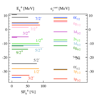
Figure 3: (Color online). Self-consistent Gorkov Green’s function calculation of ⁷⁴Ni with a realistic 2N chiral interaction Entem and Machleidt (2003). Left: spectral strength distribution for one-neutron addition (above the dashed line) and removal (below the dashed line) processes. Right: Baranger effective single-particle energies.

It is worth noting that Baranger ESPEs defined through Eqs. (10)-(12) display three fundamental properties that make them fundamentally superior to any other definition of single-particle energies used in the literature: they (i) only invoke outputs of the many-body Schrödinger equation, (ii) do not depend on the single-particle basis used to expand the many-body problem and (iii) reduce to HF single-particle energies in the HF approximation, i.e., they satisfy Koopmans’ theorem Koopmans (1934) in such a limit. Eventually, the model-independent character of Baranger ESPEs relates to the fact they can be computed unambiguously within any (re)formulation (i.e. scheme) of the nuclear many-body problem, e.g. shell model formulations, ab-initio formulations, cluster models etc.

The fact that model-independent Baranger ESPEs reduce to HF single-particle energies in the HF approximation or to standard monopole ESPEs when employing a naive filling is best seen by applying the identity von Barth and Holm (1996); Vogt et al. (2004)

$$M^{(n)}_{pq} = \langle\Psi^{\text{A}}_{0}|\{\overset{n\,\text{commutators}}{\overbrace{[\ldots[[a_{p},H],H],\ldots]}},a^{\dagger}_{q}\}|\Psi^{\text{A}}_{0}\rangle\,,$$ (13)

to $n=1$ Baranger (1970); Polls et al. (1994); Umeya and Muto (2006)

$$h^{\text{cent}}_{pq} = t_{pq}+\sum_{rs}\overline{v}^{\text{2N}}_{prqs}\,\rho^{[1]}_{sr}+\frac{1}{4}\sum_{rstv}\overline{v}^{\text{3N}}_{prtqsv}\,\rho^{[2]}_{svrt}$$

$$\equiv h^{\infty}_{pq}\,\,\,,$$

where

$$\rho^{[1]}_{pq} \equiv \langle\Psi^{\text{A}}_{0}|a^{\dagger}_{q}a_{p}|\Psi^{\text{A}}_{0}\rangle=\sum_{\mu}{V^{p}_{\mu}}^{\ast}\,V^{q}_{\mu}\,\,\,,$$ (15a)

$$\rho^{[2]}_{pqrs} \equiv \langle\Psi^{\text{A}}_{0}|a^{\dagger}_{r}a^{\dagger}_{s}a_{q}a_{p}|\Psi^{\text{A}}_{0}\rangle\,\,\,,$$ (15b)

denote one- and two-body density matrices of the correlated A-body ground-state, respectively. As Eq. (II.2) stipulates, the centroid field is equal to the one-body Hamiltonian $\mathbf{h}^{\infty}\equiv\mathbf{T}+\mathbf{\Sigma}(\infty)$ whose potential part is nothing but the energy-independent component Polls et al. (1994) of the irreducible one-nucleon self-energy $\mathbf{\Sigma}(\omega)$ of the A-body ground state that naturally arises in self-consistent Green’s-function theory. Equation (II.2) also makes clear that any many-body scheme capable of calculating $\rho^{[1]}$ and $\rho^{[2]}$ can extract the associated Baranger ESPEs, i.e. the definition is universal in that sense. Physically speaking, $\mathbf{h}^{\infty}$ represents the average one-body field seen by a nucleon in presence of correlations, i.e. not in a mean-field approximation. Taking such a simplified mean-field picture, e.g. the HF limit, one has

$$\rho^{[2]}_{pqrs}=\rho^{[1]}_{pr}\rho^{[1]}_{qs}-\rho^{[1]}_{qr}\rho^{[1]}_{ps}\,,$$ (16)

such that $\mathbf{h}^{\infty}$ reduces to the usual definition of $\mathbf{h}^{\text{HF}}$ for a 2N plus 3N Hamiltonian, which proves that $e^{\text{cent}}_{p}=e^{\text{HF}}_{p}$ in this limit.

II.3 Partitioning of one-nucleon separation energies

Let us now make the schematic partitioning introduced in Eq. (2) more precise. We need to express one-nucleon separation energies in terms of ESPEs, i.e., invert Eq. (12). In order to achieve this goal, let us confront the eigenvalue equation providing ESPEs (Eq. (11)) with the one satisfied by one-nucleon addition energies (which derives from Dyson’s equation Dickhoff and Barbieri (2004))

$$\left[\mathbf{h}^{\infty}+\left.\mathbf{\Sigma}^{\text{dyn}}(\omega)\right|_{\omega=E^{+}_{\mu}}\right]\mathbf{U}_{\mu} = E^{+}_{\mu}\,\mathbf{U}_{\mu}\,,$$ (17)

where $\mathbf{\Sigma}^{\text{dyn}}(\omega)\equiv\mathbf{\Sigma}(\omega)-\mathbf{\Sigma}(\infty)$ embodies the dynamical, i.e. energy-dependent, part of the irreducible self-energy. Equation (17) leads to

$$E^{+}_{\mu}\,\text{Tr}_{{\cal H}_{1}}\!\left[\mathbf{S}_{\mu}^{+}\right] = \text{Tr}_{{\cal H}_{1}}\!\left[\mathbf{h}^{\text{cent}}\,\mathbf{S}_{\mu}^{+}\right]+\text{Tr}_{{\cal H}_{1}}\!\left[\mathbf{\Sigma}^{\text{dyn}}(E^{+}_{\mu})\,\mathbf{S}_{\mu}^{+}\right]\,,$$

which, written in the centroid basis $\{c^{\dagger}_{p}\}$ diagonalizing $\mathbf{h}^{\infty}$, reads

$$E^{+}_{\mu} = \sum_{p}s_{\mu}^{+pp}\,e^{\text{cent}}_{p}+\sum_{pq}s_{\mu}^{+pq}\,\Sigma^{\text{dyn}}_{qp}(E^{+}_{\mu})\,.$$ (18)

For each $\mu$, $\mathbf{s}_{\mu}^{+}\equiv\mathbf{S}_{\mu}^{+}/SF_{\mu}^{+}$ denotes the reduced addition spectroscopic probability matrix whose trace over ${\cal H}_{1}$ is equal to one. For a given $\mu$, the set of diagonal matrix elements $\{\mathbf{s}_{\mu}^{+pp}\}$ thus possesses the meaning of a PDF. Equation (18) provides a rigorous partitioning of one-nucleon addition energies into an independent-particle-like contribution and a correlation contribution. Still, a given one-nucleon addition energy $E^{+}_{\mu}$ does not relate to a single ESPE such that the connection between both spectra is actually of matrix character. The independent-particle-like contribution is the sum of all ESPEs weighted by the probability for state $|\Psi^{\text{A+1}}_{\mu}\rangle$ to be obtained by adding a nucleon in the associated centroid states on top of $|\Psi^{\text{A}}_{0}\rangle$. The correlation contribution involves all matrix elements of the dynamical part of the self-energy evaluated at the one-nucleon addition energy of interest.

It is essential to stress that the partitioning (18) of the one-nucleon separation energy emerges as a direct consequence of the exact Dyson equation Dickhoff and Barbieri (2004). We have not made any assumption regarding the way the many-body problem is solved to determine the ESPEs and the dynamical self-energy. At the same time, it is important to realize that the exact partitioning (18) does not specify which effects are captured by the individual contributions, and we will demonstrate in the following that these details necessarily depend on the resolution scale $\lambda$.

II.4 Non-observability

We now come to the central point of the present study, i.e., the scale dependence and non-observable character of ESPEs. The latter derives directly from the scale dependence of spectroscopic amplitudes Furnstahl and Hammer (2002); Jennings (2011) entering the definition of the centroid Hamiltonian (Eq. (10)).

II.4.1 Description of low-energy nuclear systems

So far, our discussion was conducted under the implicit assumption that one starts from a fixed and a priori given Hamiltonian $H$. In the context of low-energy nuclear physics, one is, from the outset, dealing with an effective theory of the underlying Quantum Chromo Dynamics (QCD). In this context, the paradigm is to employ $\chi$-EFT Weinberg (1991); Ordonez et al. (1994); van Kolck (1994) whose main merits are (i) to formulate the problem at hand in terms of relevant low-energy degrees of freedom (pions and nucleons) while retaining the (chiral) symmetry (breaking) of QCD, (ii) to provide a systematic framework for constructing all relevant interactions and the operators associated with other observables, and (iii) to explain the phenomenologically observed hierarchy of nuclear interactions, i.e., 2N interactions are more important than 3N interactions, which themselves dominate 4N forces, etc. This hierarchy is generated by the power counting that organizes the infinite set of interaction terms in the $\chi$-EFT Lagrangian Bedaque and van Kolck (2002); Epelbaum et al. (2009) according to their scaling with $(Q/\Lambda_{\chi})^{\nu}$. Here, $Q$ is a characteristic momentum scale for low-momentum processes and degrees of freedom, while $\Lambda_{\chi}$, the so-called chiral-symmetry-breaking scale, denotes the hard scale that characterizes omitted degrees of freedom and drives the low-energy constants in the chiral Lagrangian. $\chi$-EFT emphasizes that any self-adjoint operator associated with an observable, including the Hamiltonian, is effective and thus depends on an intrinsic resolution scale $\Lambda_{\chi}$. At a given order in $(Q/\Lambda_{\chi})^{\nu}$, operators of interest are schematically given by

$$O\equiv\sum_{\nu}O^{(\nu)}\equiv O^{\text{1N}}+O^{\text{2N}}+\ldots+O^{\text{AN}}\,\,\,,$$ (19)

and necessarily contain up to A-body components as already alluded to above for the Hamiltonian. For instance, $V^{\text{2N}}$ first contributes to $H$ at leading order (LO) while $V^{\text{3N}}$ enters at next-to-next-to leading order (N²LO) when using Weinberg’s power counting (see, e.g., Bedaque and van Kolck (2002); Nogga et al. (2005); Epelbaum et al. (2009)).

Eventually, solving the A-body Schrödinger equation (Eq. (1)) provides not only eigenfunctions $|\Psi^{\text{A}}_{k}\rangle$ and eigenenergies $E^{\text{A}}_{k}$ of $H$ but also other quantities of interest computed through, e.g., the average value $O^{\text{A}}_{k}\equiv\langle\Psi^{\text{A}}_{k}|O|\Psi^{\text{A}}_{k}\rangle$ of associated self-adjoint operators in a given eigenstate of $H$.

II.4.2 Unitary transformation

We consider a starting nuclear Hamiltonian $H$ built within $\chi$-EFT at a given order in the employed power counting. The Hamiltonian carries an intrinsic resolution scale characterized by both $\Lambda_{\chi}$ and the regularization cutoff(s) $\Lambda_{AN}$ that is introduced by the particular scheme used to renormalize many-body amplitudes at a given chiral order.

Given this effective Hamiltonian, one is free to proceed to a unitary transformation $U(\lambda)$ over Fock space. The real variable $\lambda$ parametrizing the transformation typically denotes a momentum scale that characterizes the range of coupling between low and high momenta (within the interval defined by the intrinsic resolution scale of the starting $H$, which is itself a matter of choice) in the resulting Hamiltonian that takes the “running” form

$$H(\lambda) \equiv U(\lambda)HU^{\dagger}(\lambda)\equiv T+V^{\text{2N}}(\lambda)+V^{\text{3N}}(\lambda)+\ldots\,,$$

where $V^{\text{AN}}(\lambda)$ changes with the scale $\lambda$. Even if the starting Hamiltonian $H$ were to contain only, e.g., one and two-body operators, its unitarily equivalent partner $H(\lambda)$ would in general contain (hopefully small) higher-body operators, which eventually truncate at the A-body level when applying the Hamiltonian on the A-body Hilbert space ${\cal H}_{\text{A}}$. Applying this unitary transformation to the Schrödinger equation, we obtain

$$H(\lambda)|\Psi^{\text{A}}_{\mu}(\lambda)\rangle = E^{\text{A}}_{k}|\Psi^{\text{A}}_{\mu}(\lambda)\rangle\,,$$ (21)

where

$$|\Psi^{\text{A}}_{\mu}(\lambda)\rangle \equiv U(\lambda)\,|\Psi^{\text{A}}_{\mu}\rangle\,,$$ (22)

such that the eigenvalues $E^{\text{A}}_{k}$ remain unchanged, while the many-body wave functions run with $\lambda$. Similarly, other operators transform under $U(\lambda)$ according to

$$O(\lambda) \equiv U(\lambda)\,O\,U^{\dagger}(\lambda)\equiv O^{\text{1N}}(\lambda)+O^{\text{2N}}(\lambda)+O^{\text{3N}}(\lambda)+\ldots\,.$$

A key aspect of quantum mechanics concerns the assessment that the physical results, i.e. observables, must remain unchanged under this unitary transformation. The consistent transformation of operators and many-body wave-functions ensures that eigenspectra of transformed operators, or more generally amplitudes of transformed operators between transformed states, including many-body cross sections, are indeed invariant under $U(\lambda)$ Schuster et al. .

An issue arises whenever a quantity is defined under the assumption that the associated operator should not be transformed under $U(\lambda)$. This is the case for one-nucleon spectroscopic amplitudes that are defined at any $\lambda$ as

$$U^{p}_{\mu}(\lambda) \equiv\langle\Psi^{\text{A}}_{0}(\lambda)|a_{p}|\Psi^{\text{A+1}}_{\mu}(\lambda)\rangle\,,$$ (23a)

$$V^{p}_{\nu}(\lambda) \equiv\langle\Psi^{\text{A}}_{0}(\lambda)|a^{\dagger}_{p}|\Psi^{\text{A-1}}_{\nu}(\lambda)\rangle\,,$$ (23b)

i.e., only the many-body states involved run with $\lambda$, not the operator. As a result, spectroscopic amplitudes undoubtedly vary with $\lambda$. One may suggest to transform the operator as well in the definition of spectroscopic amplitudes in order to make them invariant by construction. The transformed operator would have the general form

$$U(\lambda)\,a^{\dagger}_{p}\,U^{\dagger}(\lambda)=\sum_{q}u^{p}_{q}(\lambda)\,a^{\dagger}_{q}+\sum_{qrs}u^{p}_{qrs}(\lambda)\,a^{\dagger}_{q}a^{\dagger}_{r}a_{s}+\ldots\,,$$ (24)

with the initial conditions $u^{p}_{q}(\lambda_{\text{init}})=\delta_{qp}$ for the first term and $u^{p}_{qrs\ldots}(\lambda_{\text{init}})=0$ for the others. Inserting such a form in the definition of the amplitudes would indeed lead to invariant spectroscopic factors and one-body centroid matrix $\mathbf{h}^{\text{cent}}$ (and thus ESPEs). However, the transformed operator (24) clearly no longer corresponds to the addition of a nucleon in a specific single-particle state. Instead, it is a linear combination of not only one-particle operators but also two-particle/one-hole operators, three-particle/two-hole operators, etc. This contradicts the initial motivation behind the introduction of spectroscopic one-nucleon addition and removal amplitudes. Indeed, spectroscopic factors and ESPEs inform on the probability and the energy generated by adding and removing a nucleon through a process that involves a single nucleon state at a time, i.e., a pure direct process. If this is not the case, ESPEs no longer reduce to HF single-particle energies in the HF limit. To conclude, defining ESPEs in the context of a change of scale necessarily leads to keeping their definition formally the same for any $\lambda$ at the price of making their actual value scale dependent. The same goes for spectroscopic factors built from $\mathbf{U}_{\mu}(\lambda)$ and $\mathbf{V}_{\nu}(\lambda)$.

II.4.3 Scale dependence

Following the spirit of the SRG Bogner et al. (2010), a unitary transformation of the resolution scale can be defined through the differential flow equations of operators and many-body wave-functions

$$\frac{d}{d\lambda}O(\lambda) \equiv \left[\eta(\lambda),O(\lambda)\right]\,,$$ (25a)

$$\frac{d}{d\lambda}|\Psi^{\text{A}}_{\mu}(\lambda)\rangle \equiv \eta(\lambda)|\Psi^{\text{A}}_{\mu}(\lambda)\rangle\,,$$ (25b)

where the anti-hermitian generator of the transformation reads

$$\eta(\lambda)\equiv\frac{dU(\lambda)}{d\lambda}U^{\dagger}(\lambda)=-\eta^{\dagger}(\lambda)\,,$$ (26)

and the initial conditions are $O(\lambda_{\text{init}})=O$ and $|\Psi^{\text{A}}_{\mu}(\lambda_{\text{init}})\rangle=|\Psi^{\text{A}}_{\mu}\rangle$. By combining Eqs. (23) and (25), one obtains the flow equations for all quantities of interest.

Starting from one-nucleon spectroscopic amplitudes

$$\frac{d}{d\lambda}V^{p}_{\nu}(\lambda) = -\langle\Psi^{\text{A-1}}_{\nu}(\lambda)|[\eta(\lambda),a_{p}]|\Psi^{\text{A}}_{0}(\lambda)\rangle^{\ast}\,,$$ (27a)

$$\frac{d}{d\lambda}U^{p}_{\mu}(\lambda) = -\langle\Psi^{\text{A+1}}_{\mu}(\lambda)|[\eta(\lambda),a^{\dagger}_{p}]|\Psi^{\text{A}}_{0}(\lambda)\rangle^{\ast}\,,$$ (27b)

one obtains flow equations for spectroscopic probability matrices $\mathbf{S}_{\mu}^{+}$ and $\mathbf{S}_{\nu}^{-}$ as well as their traces $SF^{+}_{\mu}$ and $SF^{-}_{\nu}$. Combining Eq. (27) with the fact that observable one-nucleon addition and removal energies are invariant because they are differences of eigenvalues of $H(\lambda)$ (see Eq. (21))

$$\frac{d}{d\lambda}E^{-}_{\nu}(\lambda) = \frac{d}{d\lambda}E^{+}_{\mu}(\lambda)=0\,,$$ (28)

one can eventually derive flow equations for the zeroth and first moments of the spectral function matrix

$$\frac{d}{d\lambda}\,M^{(0)}_{pq}(\lambda) = 0\,,$$ (29a)

$$\frac{d}{d\lambda}\,M^{(1)}_{pq}(\lambda) = -\langle\Psi^{\text{A}}_{0}(\lambda)|\{[[\eta(\lambda),a_{p}],H(\lambda)],a^{\dagger}_{q}\}+\{[a_{p},H(\lambda)],[\eta(\lambda),a^{\dagger}_{q}]\}|\Psi^{\text{A}}_{0}(\lambda)\rangle\,.$$ (29b)

Equation (29) demonstrates that sum rule (9) is scale invariant while the centroid matrix $\mathbf{h}^{\text{cent}}(\lambda)$ and its eigenvalues $e^{\text{cent}}_{p}(\lambda)$ are not. Just as for spectroscopic factors, the latter property underlines the scale dependence of ESPEs, i.e., they “run” with the unitary transformation $U(\lambda)$, as opposed to true observables.

II.4.4 Symmetry transformations

It is worth noting that symmetry transformations of the Hamiltonian associated with a (locally) compact Lie groups whose generators $C_{i}$ are one-body operators do not induce any running of spectroscopic factors and ESPEs. Using a one-parameter group for simplicity and employing an exponential map to represent the transformation, i.e., $U(\beta)=e^{i\beta C}$, one can show that the transformation of creation and annihilation operators in Fock space reduces to

$$U(\beta)\,a^{\dagger}_{p}\,U^{\dagger}(\beta) = \sum_{q}u_{qp}(\beta)a_{q}^{\dagger}\,,$$ (30a)

$$U(\beta)\,a_{p}\,U^{\dagger}(\beta) = \sum_{q}u^{\ast}_{qp}(\beta)a_{q}\,,$$ (30b)

where $u_{qp}(\beta)\equiv\langle q|U(\beta)|p\rangle$ is the unitary matrix representing $U(\beta)$ in the one-body Hilbert space ${\cal H}_{1}$. In contrast to Eq. (24), a transformed creation (annihilation) operator remains a linear combination of pure one-particle creation (annihilation) operators. In this case, it is straightforward to show that spectroscopic probability matrices and the centroid matrix transform as standard matrices on ${\cal H}_{1}$ by using Eq. (30)

$$S_{k}^{\pm pq}(\beta) =\sum_{rs}u_{pr}(\beta)S_{k}^{\pm rs}u^{\dagger}_{sq}(\beta)\,,$$ (31a)

$$h^{\text{cent}}_{pq}(\beta) =\sum_{rs}u_{pr}(\beta)h^{\text{cent}}_{rs}u^{\dagger}_{sq}(\beta)\,.$$ (31b)

By virtue of the unitarity of $u_{qp}(\beta)$, the spectroscopic factors, i.e., the trace of the spectroscopic probability matrices, do not depend on $\beta$. Because $U(\beta)$ is a symmetry of $H$, it is also straightforward to show that $\mathbf{h}^{\text{cent}}$ is a scalar and thus does not depend on $\beta$ either.

Ultimately, this underlines the fact that we are presently not concerned with symmetry transformations. The transformations we are interested in are, e.g., free-space SRG transformations defined through their generator $\eta(\lambda)$ in such a way that the virtual coupling between low and high momenta is continuously reduced in $H(\lambda)$ (see Ref. Bogner et al. (2010) for details). Creation and annihilation operators are transformed on Fock space according to the general law (24) and not the simpler transformation (30), which in turn causes spectroscopic factors and ESPEs to run with $\lambda$.

II.4.5 Discussion

The scale dependence of ESPEs generated by the flow equation (29b) has significant consequences. Despite the model-independent and physically intuitive character of Baranger’s ESPEs, these quantities are not observable. Like spectroscopic factors, wave-functions or “correlations”, nuclear shells do not qualify as an observable within the frame of quantum mechanics as they can be modified at will under a unitary transformation (while keeping true observables invariant). In that respect, the partitioning provided by Eq. (18) can now be further specified as

$$\overset{\text{many-body observable}}{\underset{\text{invariant under \,}U(\lambda)}{\underbrace{E^{+}_{\mu}}}}\equiv\overset{\text{single-particle components}}{\underset{\text{varies under \,}U(\lambda)}{\underbrace{\sum_{p}s_{\mu}^{+pp}(\lambda)\,e^{\text{cent}}_{p}(\lambda)}}}\,\,+\,\,\,\,\overset{\text{correlations}}{\underset{\text{varies under \,}U(\lambda)}{\underbrace{\sum_{pq}s_{\mu}^{+pq}(\lambda)\,\Sigma^{\text{dyn}}_{qp}(E^{+}_{\mu};\lambda)\,}}}\,,$$ (32)

which underlines that such a partitioning is necessarily scale dependent.

An immediate consequence of the above analysis is the realization that extracting the single-particle shell structure and its evolution, e.g., with isospin, from experimental data is an illusory objective. The single-nucleon shell structure only exists within the theoretical framework, given that experimental data determine the Hamiltonian only up to a unitary transformation $U^{\dagger}(\lambda)U(\lambda)=1$. Any quantity that intrinsically depends on $\lambda$ is undefined in the empirical world and can only acquire the status of a quasi-observable by fixing arbitrarily (but conveniently) the scale defining the Hamiltonian $H(\lambda)$ employed in the theoretical description. Still, any correlation established between an observable and a quasi-observable in an analysis performed at a particular scale may possibly disappear at another scale (see e.g. the example of Fig. 2). For instance, the claim that a given one-nucleon addition energy $E^{+}_{\mu}$ tracks a specific particle-like ESPE $e^{\text{cent}}_{p}(\lambda)$ contributing to the first term on the right-hand side of Eq. (32) can always be altered via a unitary transformation that leaves $E^{+}_{\mu}$ unchanged but that reshuffles the weight of the various terms on the right-hand side.

To fully appreciate the consequences of these statements, let us consider two practitioners independently analyzing the same (ideally) complete set of experimental data $\{E^{\pm}_{k};\sigma^{\pm}_{k}\}$ obtained from one-nucleon addition and removal experiments. Let us further postulate that they employ the same exact structure and reaction many-body theories in their analyses but two different, though unitarily equivalent, Hamiltonians $H(\lambda)$ and $H(\lambda^{\prime})$. As Eqs. (28) and (29) demonstrate, the two practitioners will both reproduce experimental observables perfectly, as $E^{\pm}_{k}(\lambda)=E^{\pm}_{k}(\lambda^{\prime})$ and $\sigma^{\pm}_{k}(\lambda)=\sigma^{\pm}_{k}(\lambda^{\prime})$, and fulfill sum-rule (9). However, they will extract two different sets of nuclear shell energies and spectroscopic factors given that $e^{\text{cent}}_{p}(\lambda)\neq e^{\text{cent}}_{p}(\lambda^{\prime})$ and $SF_{k}^{\pm}(\lambda)\neq SF_{k}^{\pm}(\lambda^{\prime})$. This must be recognized prior to discussing any additional issue associated with approximations that necessarily come into play in practice. If not, the two practitioners are likely to conclude that the difference in the extracted shell energies and spectroscopic factors reflect those unavoidable approximations instead of realizing that in a perfect world they should obtain different results. We also note that the results can be compared directly (up to approximation uncertainties) if both practicioners agree on a scale and use transformation methods like the SRG to transform their results to this agreed-upon scale. This is a well-known application of RG methods, and common practice in the discussion of parton distribution functions in hadronic physics, e.g. see Ref. Sterman et al. (1995).

III Illustrations

III.1 Many-body calculations

We perform many-body calculations for oxygen isotopes via state-of-the-art multi-reference in-medium SRG (MR-IM-SRG) Tsukiyama et al. (2011); Hergert et al. (2013a, b, 2014) and self-consistent Gorkov Green’s function many-body methods Somà et al. (2011, 2014a). From MR-IM-SRG we compute ground-state binding energies of even-even isotopes and associated ESPEs. The same quantities are computed from G-SCGF along with one-nucleon addition and removal energies to eigenstates of the neighboring odd isotopes and their associated spectroscopic factors. Calculations employ a starting Hamiltonian containing a N³LO 2N chiral interaction with a regularization cutoff $\Lambda_{\text{2N}}$=500 MeV Entem and Machleidt (2003) and a local N²LO 3N interaction Navrátil (2007) with a regularization cutoff $\Lambda_{\text{3N}}$=400 MeV. The 3N interaction low-energy constants $c_{D}$=-0.2 and $c_{E}$=0.098 are taken from a fit to the ground-state energy and the $\beta$-decay half-life of $A=3$ systems Roth et al. (2012). Calculations are performed in model spaces of 14 (G-SCGF) and 15 (MR-IM-SRG) HO shells, respectively, which guarantees convergence with respect to the single-particle basis size to within 0.1%. To manage the storage requirements of the 3N matrix elements, we only include configurations with $N_{1}$+$N_{2}$+$N_{3}\leq N^{\text{3N}}_{\text{max}}$=16 (G-SCGF) and 14 (MR-IM-SRG), where $N_{i}\equiv(2n_{i}+l+1)$ are HO single-particle energy quantum numbers. Uncertainties of G-SCGF and MR-IM-SRG due to $N^{\text{3N}}_{\text{max}}$ in the oxygen isotopes are significantly below 1%, as discussed in Refs. Somà et al. (2014b) and Hergert et al. (2013a, b), respectively.

The MR-IM-SRG calculations are performed in the so-called MR-IM-SRG(2) approximation that leads to well converged results from the many-body perspective Hergert et al. (2013b), at least as long as one employs interactions with low-momentum resolution scales. The G-SCGF calculations are performed at self-consistent second order Somà et al. (2011) in the Sc0 approximation Somà et al. (2014c) that leads to well-converged results for relative quantities Somà et al. (2014a) if low-momentum interactions are used.

Our objective is to apply a sequence of SRG transformations $U(\lambda)$ to the starting chiral Hamiltonian and study the resulting variation of the quantities of interest. Ideally, we would like to vary $\lambda$ over the largest possible interval of values, i.e. from $\lambda_{\text{init}}$ to $0$. As illustrated in Sec. III.2 below, we face two difficulties that result in breaking the unitarity of $U(\lambda)$, which complicates the illustration of the scale-dependence that is our main concern in the present work. On the one hand, many-body forces induced by the transformation need to be truncated beyond three-body operators when computing a A-body system with $A>3$. Technical limitations currently restrict free-space SRG transformation to relative two- and three-body Hilbert spaces Jurgenson et al. (2009); Roth et al. (2011); Hebeler (2012); Wendt (2013), and the inclusion of four- and higher many-body forces in many-body calculations is an even bigger technical challenge. In order to prevent this truncation from inducing a too-significant breaking of unitarity, we have to keep the scale $\lambda$ of the Hamiltonian sufficiently large. On the other hand, the employed ab initio methods introduce truncations of the many-body expansion. At their current level of implementation, the resolution scale $\lambda$ of the Hamiltonian must be sufficiently small to ensure that the contribution of the truncated terms of the many-body expansion does not exceed the desired accuracy for the calculated observables, which is on the level of 2-3% in oxygen. To accommodate these two opposing constraints, we are currently forced to work in a limited interval of resolution scales encompassing the three values $\lambda=1.88,2.00,2.24$ fm^-1 used in this work. Nevertheless, we will demonstrate below that this range is sufficient to illustrate the formal arguments provided above. Obviously, the quality of the illustrations proposed below can be improved in the future if (i) the SRG transformation can be conducted in Hilbert spaces ${\cal H}_{A}$ with $A>3$, (ii) four- and higher-body forces can be handled in many-body calculations and if (ii) the many-body truncations enforced within MR-IM-SRG and G-SCGF theories reach a maturity ensuring the convergence of calculations based on Hamiltonians characterized by a large resolution scale $\lambda$.

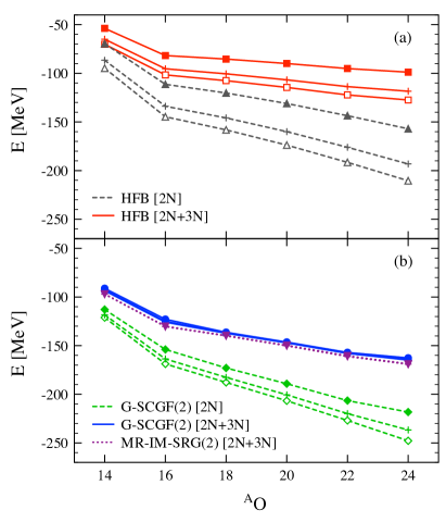
Figure 4: (Color online). Ground-state binding energies of ^14-24O computed for $\lambda=1.88$ (open symbols), $2.00$ (crosses), and $2.24$ fm^-1 (filled symbols). Panel (a): lowest order (i.e. HFB) calculation for two cases: keeping the sole 2N interaction and incorporating both starting and induced 3N interactions. Panel (b): G-SCGF second-order results without and with 3N forces (as above) and MR-IM-SRG(2) calculation with the full 2N+3N Hamiltonian.

III.2 Breaking unitarity

In order to qualify the intrinsic running of non-observable ESPEs and spectroscopic factors, one must quantify the (presently) unavoidable, though artificial, scale dependence of observables in any practical calculation. As already alluded to, the latter originates from the breaking of unitarity due to (i) the omission of induced many-body forces beyond $A=3$ and (ii) truncations of the many-body expansion when the many-body Schrödinger equation is solved.

Given that we use a finite interval of scale variation, it is difficult to characterize the extent of this artificial scale dependence of observables in an absolute sense. In order to provide some perspective, we first alter our G-SCGF calculations by retaining 2N interaction only (thus omitting all many-body interactions induced from it including the 3N operator) and/or by degrading the self-consistent second-order treatment to the strict Hartree-Fock-Bogoliubov (HFB) level that acts as a zeroth-order baseline. The corresponding results are displayed in Fig. 4 for the ground-state binding energy of ^14-24O.

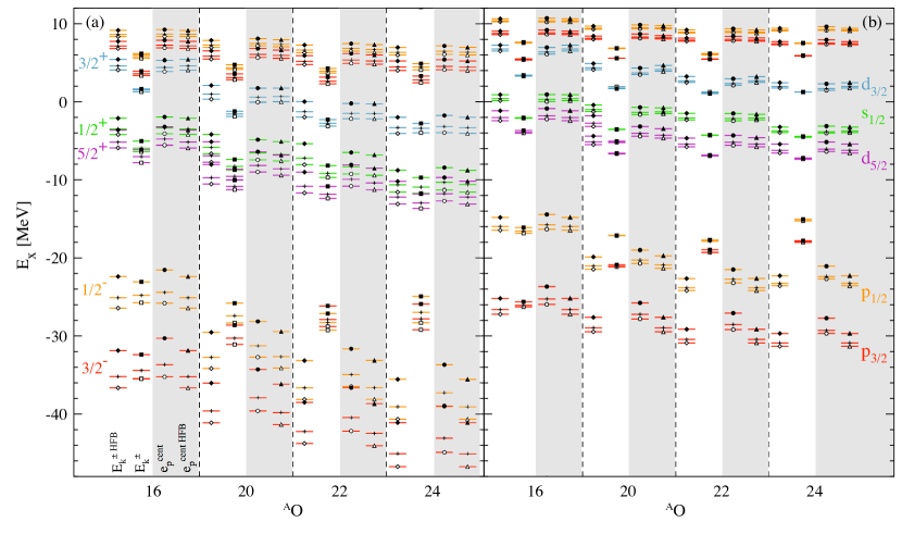
Figure 5: (Color online) One-neutron separation energies with dominant spectroscopic factors versus neutron ESPEs in ^16,20,22,24O. Each level is displayed for $\lambda=1.88$ (open symbols), $2.00$ (crosses), and $2.24$ fm^-1 (filled symbols). Results are displayed for both HFB and second-order G-SCGF calculations. Panel (a): one- and two-body operators are retained in the initial and transformed Hamiltonians. Panel (b): one-, two-, and three-body operators are retained in the initial and transformed Hamiltonians.

First, the scale dependence generated over the interval $\lambda\in[1.88,2.24]$ is systematically smaller in the calculations that keep 2N and 3N operators than in the calculation only retaining the 2N interaction. Second, the reduced scale dependence is very significant in both calculations when going from HFB to self-consistent second order. Using 2N+3N forces for example, the scale dependence is reduced from about 20-30 MeV to typically 2 MeV when spanning the (small) interval $\lambda\in[1.88,2.24]$ fm^-1, i.e. by a factor $\sim 15$. Note, however, that part of the reduction is due to a cancellation between induced 4N interactions from the initial 2N and 3N interactions, as discussed in Refs. Binder et al. (2013c); Hergert et al. (2013a, b); Binder et al. (2013b).

In order to verify that the pattern just discussed is not specific to G-SCGF but reflects a generic aspect of the many-body problem, we further compare in panel (b) of Fig. 4 with MR-IM-SRG(2) calculations for the Hamiltonian containing 2N+3N forces. At the current level of implementation, the MR-IM-SRG includes many-body terms beyond G-SCGF, and allows an even more significant reduction of the scale dependence, while also benefitting from the cancellation of induced 4N terms mentioned above. The residual running ranges from $50$ keV in ${}^{14}\mathrm{O}$ to $400$ keV in ${}^{24}\mathrm{O}$ for $\lambda\in[1.88,2.24]$ fm^-1. The better many-body convergence of MR-IM-SRG(2) is also reflected in the additional absolute binding Somà et al. (2014a); Hergert et al. (2014). A third-order G-SCGF truncation scheme will provide the missing binding energy and will allow for a further attenuation of the scale dependence, as shown in Ref. Cipollone et al. (2013) for closed-shell oxygen isotopes.

III.3 Nuclear shell energies

First, we compare one-nucleon separation energies $E^{\pm}_{k}$ with absolute ESPEs $e^{\text{cent}}_{p}$ in ^16,20,22,24O. For each spin and parity, we consider the separation energy of the state with the dominant strength. As in the previous section, we perform HFB and G-SCGF calculations using the SRG-evolved 2N and 2N+3N Hamiltonians, and compile results from all four variants in Fig. 5, covering energies from $-48$ MeV to $+10$ MeV. Let us now list the main lessons one can learn from these results.

• Combining panels (a) and (b), one can appreciate the significant reduction of the artificial scale dependence of all one-nucleon separation energies obtained by keeping 3N operators in the Hamiltonian and/or by going from HFB to second-order G-SCGF.

• The running of ESPEs is qualitatively different and quantitatively larger than for observable one-nucleon separation energies. This is particularly clear for the 2N+3N Hamiltonian: While the average spread of all displayed separation energies is equal to $0.2$ MeV for $\lambda\in[1.88,2.24]$ fm^-1, the average spread of ESPEs is equal to $1.1$ MeV. The distribution of those spreads is shown in detail in Fig. 6.

• While the spread of ESPEs is qualitatively different and quantitatively larger than that of observable one-nucleon separation energies, it is worth mentioning that the latter are much more sensitive to correlations than the former. Indeed, while the values of a given separation energy computed for $\lambda\in[1.88,2.24]$ fm^-1 converge towards one another when going from HFB to self-consistent second-order, each of them does so by changing significantly on an absolute scale. This systematic convergence of the one-nucleon separation energies computed for three different scales to a common value as one improves the many-body treatment is not fortuitous but rather reflects the intrinsic scale independence of these observables. This trend is qualitatively different for ESPEs whose genuine spread ultimately remains similar (and significant) when going from HFB to self-consistent second order.

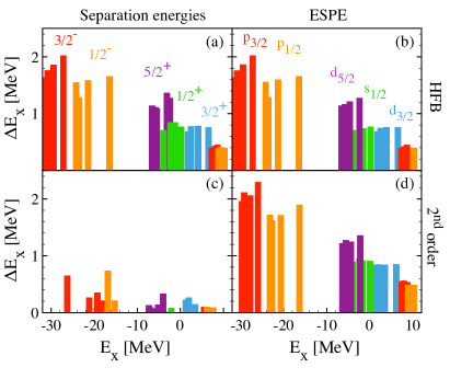
Figure 6: (Color online) Residual spreads of separation energies and ESPEs in HFB and second-order G-SCGF calculations with a 2N+3N Hamiltonian. Differences between $\lambda=1.88$ and $2.24$ fm^-1 calculations are displayed for each spin-parity state. For one-neutron separation energies, states with spectroscopic factor larger than $30\%$ are retained. All states displayed in Fig. 5(b) are plotted indistinctly. Going from panel (a) to panel (c), one notices (i) a large reduction of the scale dependence and (ii) the expected compression of the strength due to the inclusion of the coupling to fluctuations. Comparing panels (b) and (d) makes clear that none of these two features is reflected in the ESPEs, i.e. in the underlying shell structure.

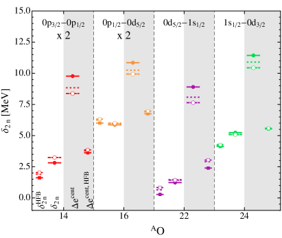
Figure 7: (Color online) Two-nucleon shell gap versus the ESPE Fermi gap in ^14,16,22,24O. Each quantity is displayed for $\lambda=1.88$ (dashed lines, open symbols), 2.00 (dotted lines, no symbols), and 2.24  fm^-1 (solid lines, filled symbols). Results are displayed for both HFB ($\delta^{\text{HFB}}_{2n},\Delta e^{\text{cent,HFB}}$) and the MR-IM-SRG(2) ($\delta_{2n},\Delta e^{\text{cent}}$) truncation scheme. One-, two-, and three-body operators are retained in the initial and transformed Hamiltonians.

Second, we compare in Fig. 7 HFB and MR-IM-SRG(2) results for the so-called two-neutron shell gap and the ESPE gap across the Fermi energy, focusing on the nuclei ^14,16,22,24O that display good closed sub-shell character for the 2N+3N Hamiltonian (e.g., there is no pairing at the HFB level). The observable two-neutron shell gap and the ESPE gap are defined through Bender et al. (2006, 2008)

$$\delta_{2n}(N,Z) \equiv\frac{1}{2}\left(E(N\!+\!2,Z)-2E(N,Z)+E(N\!-\!2,Z)\right)\,,$$ (33)

and

$$\Delta e^{\text{cent}}(N,Z) \equiv e^{\text{cent}}_{p}(N,Z)-e^{\text{cent}}_{h}(N,Z)\,,$$ (34)

respectively. By definition $e^{\text{cent}}_{h}(N,Z)$ ($e^{\text{cent}}_{p}(N,Z)$) denotes the ESPE energy of the last occupied (first empty) shell obtained via a naive, i.e. non interacting, filling of those shells for the even-even system with $N$ neutrons and $Z$ protons. Disregarding the change in the single-particle wave functions when going from $N$ to $N\pm 2$ nuclei, along with the interaction between the added (removed) two neutrons, it is easy to see that $\delta_{2n}(N,Z)$ and $\Delta e^{\text{cent}}(N,Z)$ are equal in the HF limit. This is the reason why the former observable is often compared to the latter non observable ESPE gap.

The main lessons to retain from Fig. 7 are similar to before.

• As expected from good doubly-closed shell systems, the ESPE Fermi gap captures the two-neutron shell gap quantitatively at the mean-field, i.e. HFB, level independently of the scale used. Contrarily, this is not at all the case at the MR-IM-SRG(2), i.e. correlated, level. This is typical of ab-initio theoretical schemes where the dynamics of all nucleons is treated on the same footing, as was already exemplified above for one-nucleon separation energies from second-order G-SCGF calculations as well as from CC calculations at the singles and doubles level in Ref. Duguet and Hagen (2012).

• The scale dependence of the ESPE Fermi gap is qualitatively different and systematically larger than the artificial running of the two-neutron shell gap, thus illustrating the non-observable (observable) nature of the former (latter). The scale dependence of $\delta_{2n}(N,Z)$ is reduced systematically from $600-700\,\,\text{keV}$ to $200\,\,\text{keV}$ by going from HFB to MR-IM-SRG(2), with the exception of ${}^{14}\mathrm{O}$, where the $\delta_{2n}(N,Z)$ obtained from HFB and MR-IM-SRG(2) are both $\sim 850\,\,\text{keV}$. In contrast, the scale dependence of the ESPE Fermi gap grows from $400-600\,\,\text{keV}$ to $1.5-2.8\,\,\text{MeV}$ in ${}^{14,16,22}\mathrm{O}$ as we go from HFB to MR-IM-SRG(2).

The above results constitute the best illustration currently allowed by state-of-the-art many-body calculations of the scale dependence of nuclear shell energies. While we consider this illustration to be already striking, its quality will keep improving over the coming years, as already mentioned in Sect. III.B.

III.4 Spectroscopic factors

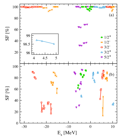
Figure 8: (Color online) Spectroscopic factors associated with one-neutron addition and removal process on the ground states of ^{14,16,18,20,22,24}O computed as a function of the associated separation energy. For each final state, results obtained for $\lambda=1.88,2.00,2.24$ fm^-1 are joined by solid lines. One-, two-, and three-body operators are retained in the (initial and) transformed Hamiltonians. Panel (a): results obtained at the HFB level. Panel (b): results obtained from second-order G-SCGF calculations.

Let us also briefly illustrate the non-observable character of spectroscopic factors. To do so, spectroscopic factors associated with one-neutron addition and removal processes on the ground states of ^{14,16,18,20,22,24}O are compiled in Fig. 8 as a function of the separation energy of the corresponding final state. For each state, the results obtained for $\lambda=1.88,2.00,2.24$ fm^-1 are connected by lines. At the HFB level (Fig. 8(a)), the variation of the spectroscopic factors with $\lambda$ is sufficiently small to be obscured by the symbols. This variation essentially occurs horizontally because the one-neutron separation energies do depend on $\lambda$ (see inset in Fig. 8(a)) at that level as discussed previously. Contrarily, there is essentially no vertical variation as one is operating within an independent (quasi)-particle picture such that the strength for particle addition or removal is contained almost entirely in individual single-particle states, i.e. the eigenstates of $\mathbf{h}^{\text{cent}}$, by construction. Spectroscopic factors are actually not strictly equal to 1 (or 0) due to the treatment of pairing correlations in the HFB framework, the two $5/2^{+}$ states associated with one-neutron addition and removal in the open-shell ²⁰O being the most prominent example.

The picture is different in Fig. 8(b), where results from second-order G-SCGF calculations are compiled. There is less variation along the horizontal axis than in the HFB case because the improved many-body treatment reduces the scale dependence of the observable one-neutron separation energies (cf. Fig. 5). Due to the inclusion of dynamical correlations, the spectroscopic strength is now fragmented. For certain states, in particular the $1/2^{-}$ and $3/2^{-}$ states, the vertical spread becomes visible and indicates that the details of this fragmentation depend on the resolution scale $\lambda$ (while the associated separation energy does not). By improving the treatment of the many-body problem through switching from HFB to G-SCGF, we have thus slightly increased the scale dependence of some of the non-observable spectroscopic factors significantly. Still, a larger range of $\lambda$ values will have to be used in order to generate any significant and systematic scale dependence.

IV Conclusions

The present work is dedicated to specifying and illustrating the non-observable nature of the one-nucleon shell structure. After a formal demonstration, state-of-the-art multi-reference in-medium similarity renormalization group and self-consistent Gorkov Green’s function many-body calculations based on chiral two- and three-nucleon interactions are employed to illustrate that, as opposed to observable quantities, nuclear shell energies run under unitary similarity renormalization group transformations of the Hamiltonian parameterized by the resolution scale $\lambda$. In practice, the unitarity of the similarity transformations is broken due to the omission of induced many-body interactions in the present framework, and the approximate treatment of the Schrödinger equation. The impact of this breaking is first characterized by quantifying the (artificial) running of observables over a (necessarily) finite interval of $\lambda$ values. Then, the (genuine) running of ESPEs is characterized and shown to be convincingly larger than that of observables (which would be zero in an exact calculation).

The non-observable nature of the nuclear shell structure, i.e., the fact that it constitutes an intrinsically theoretical object with no counterpart in the empirical world, must be recognized and assimilated. Indeed, the shell structure cannot be extracted from experimental data; hence it cannot be talked about in an absolute sense as it depends on the non-observable resolution scale employed in the theoretical calculation. Consequently, correlations that one may establish between observables, e.g., first $2^{+}$ excitation energies or one-nucleon separation energies, and features of the shell structure, e.g., the size of the particle-hole gap at the Fermi energy, depend on the resolution scale. It is only at the price of fixing arbitrarily (but conveniently!) the resolution scale in the theoretical framework that one can establish and utilize such correlations. To some extent, fixing the resolution scale provides ESPEs (and spectroscopic factors) with a quasi-observable character.

Ultimately, practitioners can refer to nuclear shells and spectroscopic factors in their analyses of nuclear phenomena. This however requires that it is done on the basis of a well defined theoretical scheme, i.e. well specified degrees of freedom combined with a Hamiltonian characterized by a fixed resolution scale. It is mandatory to perform comparisons from one nucleus to the other or from one practitioner to the other on the basis of that very same theoretical scheme. Incidentally, this also necessitates to use consistent structure and reaction theoretical schemes, i.e. structure and reaction theories based on the same degrees of freedom and the same fixed Hamiltonian, eventually employing the same approximations within that many-body scheme. This is of course a very challenging task for the future. Still, it indicates that, from the perspective of future theoretical developments, there is not much value in combining, e.g., high-quality ab initio nuclear structure quantities with inconsistent nuclear reaction theories. The focus should rather be on consistency as there is more value in developing less advanced, e.g. less ab initio, structure and reaction theories as long as the degrees of freedom, the many-body truncation schemes and the nuclear Hamiltonian underlying both are consistent.