A feedback-driven bubble G24.136+00.436: a possible site of triggered star formation

Abstract

We present a multi-wavelength study of the IR bubble G24.136+00.436. The J=1-0 observations of ¹²CO, ¹³CO and C¹⁸O were carried out with the Purple Mountain Observatory 13.7 m telescope. Molecular gas with a velocity of 94.8 km s^-1 is found prominently in the southeast of the bubble, shaping as a shell with a total mass of $\sim 2\times 10^{4}$ $M_{\odot}$. It is likely assembled during the expansion of the bubble. The expanding shell consists of six dense cores. Their dense (a few of $10^{3}$ cm^-3) and massive (a few of $10^{3}$ $M_{\odot}$) characteristics coupled with the broad linewidths ($>$ 2.5 km s^-1) suggest they are promising sites of forming high-mass stars or clusters. This could be further consolidated by the detection of compact HII regions in Cores A and E. We tentatively identified and classified 63 candidate YSOs based on the Spitzer and UKIDSS data. They are found to be dominantly distributed in regions with strong emission of molecular gas, indicative of active star formation especially in the shell. The HII region inside the bubble is mainly ionized by a $\sim$O8V star(s), of the dynamical age $\sim$1.6 Myr. The enhanced number of candidate YSOs and secondary star formation in the shell as well as time scales involved, indicate a possible scenario of triggering star formation, signified by the “collect and collapse” process.

1. Introduction

It is believed that the majority of stars in Galaxy form in clusters. The feedback from them is expected to have strong influences on their neighbor interstellar mediums (ISMs). Massive stars residing in a cluster deposit large amounts of energies into ambient molecular clouds in the form of strong ultraviolet (UV) radiation (h$\nu>$ 13.6 ev) which photoionizes surrounding gas, creating bubbles/HII region. The expanding bubbles/HII regions likely prompts the collapse of molecular clouds which may not contract and fragment spontaneously, and stimulates star formation of next generations. This process is defined as triggered star formation.

Scenarios of triggered star formation have been suggested by a few theoretical models and several observations. For example, Elmegreen & Lada (1977) first proposed a “collect and collapse” process. It could be described as follows: as an HII region expands outwards, its surroundings may be compressed and collected between the ionization front (IF) and the shock front (SF); the shell between the IF and SF in due time may become dense, massive and gravitationally unstable, and collapse to form new stars. If this process occurs, it would self-propagate and lead to sequential star formation. Several simulations concluded that the expanding HII region or ionizing feedback should be an efficient trigger for star formation in molecular clouds if the mass of the ambient molecular material is massive enough (Hosokawa & Inutsuka, 2005, 2006; Dale et al., 2007, 2012, 2013). Observational signatures of this process have been presented on boundaries of several HII regions where the number of young stellar objects (YSOs) is enhanced (e.g. Deharveng et al. (2005); Pomarès et al. (2009); Liu et al. (2012)).

Other existing observations also showed the prevalence of triggering star formation in the Milky Way. For example, Thompson et al. (2012) studied the association of Red MSX massive young stellar objects (MYSOs) with the 322 bubbles from the Churchwell et al. (2006) catalog. The result suggested that around $14\%-30\%$ of massive stars in the Milky Way might have been triggered by the expansion of the bubbles. Similarly, from the association of MYSOs with $1018$ Milky Way Project bubbles (visually identified by citizen scientists (Simpson et al., 2012)), Kendrew et al. (2012) found that approximately $22\%\pm 2\%$ of MYSOs might have been induced by feedback from the expanding bubbles/HII regions. Additionally, by combining the geometry of stars and surviving cold ISMs, some possible signatures of triggered star formation have been reported over a number of known HII regions, such as Sh2$-212$ (Deharveng et al., 2008), W51a (Kang et al., 2009), Sh2$-217$ (Brand et al., 2011), and Sh2$-90$ (Samal et al., 2014). These results suggested that IR bubbles or HII regions could serve as a good laboratory for the study of triggered star formation. However, the exact processes of interactions between bubbles/HII regions and the ambient ISMs remain unclear. Hopefully, the investigation of the physical connection and interaction of bubbles/HII regions with their adjacent ISMs would achieve a better understanding of star formation around bubbles/HII regions (Samal et al., 2014).

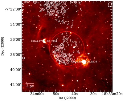
Figure 1.— 8.0 $\mu$m image of G24.136 overlaid with contours of free-free emission at 20 cm. The contours start from $5\sigma$ ($\sigma=0.15$ mJy/beam) in a step of $1\sigma$. The image with a size of $12\arcmin\times 12\arcmin$ is centered at $\alpha=18^{\mathrm{h}}33^{\mathrm{m}}43.94^{\mathrm{s}},\delta=-07\arcdeg 36\arcmin 52.8\arcsec$. The circle characterizes the radius of the bubble, 2.3$\arcmin$, which corresponds to 3.9 pc at a distance of 5.6 kpc. A scale bar of 2 pc is shown on the bottom left.

The purpose of this work is to probe the evidence of triggered star formation and investigate formation of massive stars or clusters as well as star formation histories around the bubbles. Therefore, we carried out a multi-wavelength study towards the bubble MWP1G024.136+00.436 (Simpson et al. (2012), G24.136 hereafter), located at $18^{\mathrm{h}}33^{\mathrm{m}}43.96^{\mathrm{s}},\delta=-07\arcdeg 37\arcmin 15.5\arcsec$. This paper is organized as follows: the region of G24.136 is presented in Sect. 2; the observations of J=1-0 transitions of ¹²CO (1-0), ¹³CO (1-0) and C¹⁸O (1-0) and the archival infrared and radio data are described in Sect. 3; the result is provided in Sect. 4; the discussion is arranged in Sect. 5; the last section is the summary.

2. Presentation of G24.136

In Fig. 1, the bubble G24.136 appears to be a complete ring (red circle) as seen in the 8 $\mu$m image. The 8 $\mu$m emission predominantly comes from two prominent polycyclic aromatic hydrocarbons (PAHs) at 7.7 and 8.6 $\mu$m, which are indicative of photodissociation regions (PDRs). Since PDRs are possible nurseries of massive star or cluster formation (Zavagno et al., 2010), the bright ring consisting of PDRs demonstrates possibly rich activities of star formation in G24.136. The free-free continuum emission from ionized regions almost fills the bubble. This picture is greatly consistent with the fact that the bubble shrouds the HII region G024.139+0.427 (Lockman et al., 1996). Additionally, the region in the northeast to G24.136 is also full of the free-free radiation, indicating another HII region. We are not sure whether this region is located at the same distance as the bubble due to lacking more information (e.g., kinetic information), therefore, exclude it from further analysis. In the edge of G24.136 two compact bright PDRs are consistent with conspicuously strong free-free emission. One of the compact sources located at the southwest, G024.0953+00.4579, is classified as an HII region by Urquhart et al. (2009) with the 6 cm continuum VLA survey. The other compact source G024.1754+00.3994 is located at the northeast . In Sect. 5.3 we will confirm that these two regions are indeed compact HII (CHII) regions. The classical HII region G024.139+0.427 with its two neighboring CHII regions shows a multi-generation of star formations. There are also some regions in the rim of G24.136 seen as absorption in the 8 $\mu$m image. The associated ¹²CO (1-0) and ¹³CO (1-0) emission (Fig. 4) suggests they lie behind the cold gas.

Adopting the Brand & Blitz (1993) rotation curve, the systemic velocity, $V_{lsr}=94.1$ km s^-1, yielded a distance of $5.2\pm 1.0$ kpc (Urquhart et al., 2011). Similarly, assuming the McClure-Griffiths & Dickey (2007) rotation curve, the systemic velocity, $V_{lsr}=98.4$ km s^-1 , resulted a distance of $5.9\pm 1.0$ kpc (Anderson et al., 2009). In this work, we adopt the mean value of both distances, $5.6\pm 1.0$ kpc. Therefore, a radius of 2.3^′ (Simpson et al., 2012) of G24.136 corresponds to $3.9\pm 0.7$ pc.

3. Observations and Archival Data

3.1. Millimeter Line Observations

The observations of J=1-0 of ¹²CO, ¹³CO and C¹⁸O were made in May, 2013 using the Purple Mountain Observatory 13.7m telescope in Delingha, China. The telescope was configured with an SIS superconducting receiver consisting of a nine-beam array in the front end. ¹²CO and its isotopologues were observed simultaneously with excellent positional registrations and calibrated at the upper sideband (USB) and the lower sideband (LSB) respectively. Pointing and tracking accuracies were better than 5$\arcsec$. The backend was composed of an FFT spectrometer with 1 GHz bandwidth and 16384 channels. The corresponding velocity resolutions are 0.16 km s^-1 for ¹²CO (1-0), 0.17 km s^-1 for ¹³CO (1-0) and C¹⁸O (1-0) lines, respectively. The half-power beamwidth was about 54$\arcsec$ and the main beam efficiencies at observed frequencies were 0.44 (115.271202 GHz) and 0.48 ((110.201353 GHz) respectively. The On-The-Fly (OTF) mapping mode was adopted. Maps were made with the beam center running on a 12$\arcmin$ $\times$ 12$\arcmin$ region centered at $\alpha=18^{\mathrm{h}}33^{\mathrm{m}}43.94^{\mathrm{s}},\delta=-07\arcdeg 36\arcmin 52.8\arcsec$. The scan rate was 50$\arcsec$ per second and the integrated time was 0.3 s. To improve the ratio of signal to noise, six observations were performed on the same region. During the observations, the system temperatures ranged from 370 to 430 K for the USB and from 250 to 270 K for the LSB. After observations, all OTF data were merged into a data cube with a grid spacing of 30$\arcsec$. The antenna temperatures were converted into main-beam brightness temperatures. The RMS noise levels of the resulting data were $\sim$0.6 K for ¹²CO (1-0), and $\sim$0.3 K for ¹³CO (1-0) and C¹⁸O (1-0) lines. The resulting data were analyzed and visualized with the software GILDAS (Guilloteau & Lucas, 2000).

3.2. Archival Data

The GLIMPSE survey (Benjamin et al., 2003) had mapped portions of the inner Galactic plane, using Infrared Array Camera (IRAC) (Fazio et al., 2004) aboard the Spitzer Space Telescope. From the GLIMPSE Spring ’07 Archive, 10509 point sources over the region of $12\arcmin\times 12\arcmin$ were retrieved, which are complete to a magnitude of 14.3 mag at 3.6 $\mu$m, 14.9 mag at 4.5 $\mu$m, 12.6 mag at 5.6 $\mu$m and 12.0 mag at 8.0 $\mu$m, respectively. The images of four IRAC bands of G24.136 were also used to reveal its physical characteristics. The 24 $\mu$m image of G24.136 was obtained from MIPSGAL, another survey of the inner Galactic plane using the Multiband Imaging Photometer for Spitzer (MIPS) instrument (Rieke et al., 2004). The point sources were extracted from the image using the DAOPHOT package of software IRAF (the detailed descriptions of photometry are prepared in later work (Liu et al. 2014, in preparation)). We found 63 MIPS objects match the IRAC sources within a $2\arcsec$ search radius. These MIPS sources are completed to 8.5 mag at 24 $\mu$m. Additionally, deep near-infrared (NIR) point sources were retrieved from the UKIDSS 6th data release of Galactic Plane Survey (GPS) (Lucas et al., 2008; Lawrence et al., 2007). There were 3184 UKIDSS sources matched well with IRAC counterparts within the $2\arcsec$ radius. These NIR sources are complete to a magnitude of 14.5 mag, 15.0 mag and 14.0 mag in the $J$, $H$, and $Ks$ band, respectively.

To calculate the Lyman continuum photons from the central region of G24.136, we used radio continuum emission at 20 cm from MAGPIS (Helfand et al., 2006). To correct for the deficiency of missing fluxes, MAGPIS combined VLA images with those from a 1.4 GHz survey performed with the Effelsberg 100 m telescope (Reich et al., 1990). As a result, a better resolution of $5.4\arcsec$ and 1$\sigma$ sensitivity of $<0.15$ mJy were achieved.

4. Results

4.1. Molecular Emission

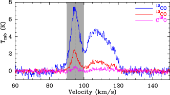
Figure 2.— The averaged spectra of ¹²CO (1-0), ¹³CO (1-0), C¹⁸O (1-0) over a region of 12 $\arcmin$ $\times$ 12 $\arcmin$ centered at $\alpha=18^{\mathrm{h}}33^{\mathrm{m}}43.94^{\mathrm{s}},\delta=-07\arcdeg 36\arcmin 52.8\arcsec$. The black dashed line represents a systemic velocity of 94.8 km s^-1. The darker shade marks the narrow-velocity component with an interval from $90$ km s^-1 to 100 km s^-1.

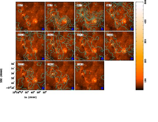
Figure 3.— The channel map (contours) of ¹²CO (1-0) overlaid on the 8 $\mu$m image (color scale). The contour levels start from $5\sigma$ ($\sigma=0.6$ K km s^-1) in a step of $3\sigma$. The velocity of the channel is plotted at the upper-right of each panel. The units of the 8 $\mu$m image is MJy/sr. The blue filled circle on the bottom right shows an angular resolution of $54\arcsec$.

Figure 2 displays the averaged spectra of ¹²CO (1-0), ¹³CO (1-0) and C¹⁸O (1-0) over the region of 12$\arcmin$ $\times$ 12$\arcmin$. It clearly portrays a narrow-velocity component, accompanying with a broad-velocity component. Based on the ¹³CO (1-0) average spectrum, their velocities range from $90$ km s^-1 to 100 km s^-1 and from $100$ km s^-1 to 120 km s^-1, respectively.

The narrow-velocity component emission is around a systemic velocity of 94.8 $\pm$ 0.42 km s^-1 (see Fig. 2), from the ambient environments of G24.136 (Anderson et al., 2009). The present systemic velocity is well consistent with that derived from the radio recombination line (Lockman et al., 1996). This supports the association of molecular gas in the interval from $90$ km s^-1 to 100 km s^-1 with the bubble. Figure 3 present the channel maps of ¹²CO (1-0) overlaid on the 8 $\mu$m image. It is clear that the emission of the narrow-velocity component is enhanced in the ring-like structure. The velocities along the NW-SE of the bubble show a systemic variance. It is still unclear whether this variance is due to projecting effects, “rocket” effects from massive stars, or some others.

The broad-velocity component appears to be projected on the bubble as an irregular morphology (see Fig. 3). Its spatial distribution is similar to that of the narrow-velocity component, showing the prominent emission in the southeastern edge of the bubble. This suggests both components may reveal the same region. However, emission of the broad-velocity component is much weaker than that of the narrow-velocity component. Figure 2 shows the non-Gaussian profile of the broad-velocity component. Apart from this, its emission intensities and profiles conspicuously vary in different positions (see Fig. 5). These features are similar to those of the supernova remnant (SNRs) seen by CO and other tracers (e.g., IC443 (Denoyer, 1979; Wang & Scoville, 1992; Zhang et al., 2010; van Dishoeck et al., 1993), W44 (Seta et al., 2004) and W28 (Arikawa et al., 1999)). van Dishoeck et al. (1993) proposed that rapid variations in line profiles from position to position probably indicate the inhomogeneous composition of the preshocked gas and the gas likely undergoing more than one shock. In this context, the broad-velocity component of G24.136 may trace shocked gas induced by the expanding bubble. However, this is a complex region with many star forming regions. On the one hand, at the Northern side of the bubbles there are three clear velocity peaks between 90 and 120 km s^-1 instead of a narrow component along with a broad one. On the other hand, the location of the bubble at $l\sim 24\arcdeg$ is roughly towards the Scutum-Centaurus tangent point near the end of the long bar in the Galaxy. Therefore, the line profile may also be simply a result of blended lines at different velocities. The lacking of more information on the broad-velocity component makes the determination of its origin and nature difficult. As a result, we focus on the narrow velocity component in the following analysis.

4.2. Dense Molecular Cores

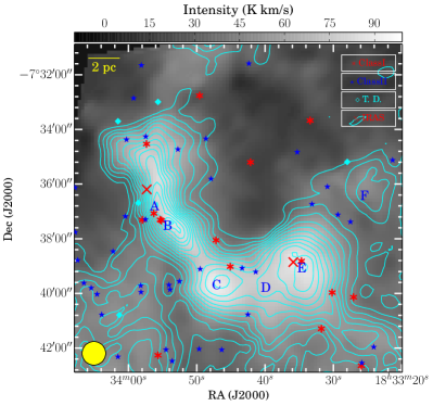
Figure 4.— ¹³CO (1-0) velocity-integrated contours overlaid on the ¹²CO (1-0) integrated map (gray scale). The velocity covers 90 km s^-1 to 100 km s^-1. Levels of the contour of ¹³CO (1-0) emission start from $10\sigma$ ($\sigma=0.7$ K km s^-1) with a step of $3\sigma$. Molecular cores are denoted as “A” to “F”. The red asterisks represent Class I YSOs, the blue stars Class II YSOs, the cyan diamonds transition disks sources, and the red crosses IRAS sources. The yellow filled circle on the bottom left displays an angular resolution of $\theta_{\mathrm{beam}}=54^{\prime\prime}$. A scale bar of 2 pc is shown on the top left.

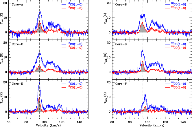
Figure 5.— The spectra of ¹²CO (1-0) and ¹³CO (1-0) at the peaks of six cores. The black dashed lines represent a systemic velocity of 94.8 km s^-1. The core names are labeled on the top left of each panel. The darker shades show the narrow-velocity component with an interval from $90$ km s^-1 to 100 km s^-1.

Figure 4 presents the ¹²CO (1-0)  integrated map overlaid with contours of ¹³CO (1-0)  intensity. The ¹²CO (1-0) emission evidently shows a molecular ring around the infrared bubble. The south-east part is dense and extensive while the north-west is diffuse and rarefied. The spatial distribution of ¹³CO (1-0) is not as extended as that of ¹²CO (1-0), indicating that the ¹³CO (1-0) transition traces more denser regions than ¹²CO (1-0). In the southeast edge of the bubble the dense region sculpted as a shell suggests that it may be gathered during the expansion of the bubble.

Figure 4 shows that the expanding shell consists of several substructures, whereby we extracted them from the map of the ¹³CO (1-0) integrated intensity using the 2D Clumpfind algorithm (Williams et al., 1994). Clumpfind searches for local peaks of emission and uses closed contours at lower intensity levels to assign boundaries. Taking the contour levels used in Fig. 4 as the inputting parameters, Clumpfind yielded six cores within the shell. They are marked as “A”,“B”,“C”,“D”, “E”, “F” hereafter. Their parameters are tabulated in Table 1, 2. We also measured the peak velocity ($V_{\mathrm{peak}}$), linewidth ($\triangle V$), and main-beam temperature ($T_{\mathrm{mb}}$) of the six cores using the software GILDAS. The corresponding spectra of the six cores are shown in Fig. 5. The peak velocities of all cores but Core F coincide well with the systemic velocity. However, the peak velocity of Core F is obviously blueshifted, which is attributed to the systemic variance aforementioned.

Table 1Observed Parameters of ¹³CO Cores

				12CO (1-0)			13CO (1-0)
Name	R.A.	DEC.	$R_{eff}$	$V_{\mathrm{LSR}}$	$\triangle V(^{12}\mathrm{CO})$	$T_{\mathrm{mb}}(^{12}\mathrm{CO})$	$V_{\mathrm{peak}}$	$\triangle V(^{13}\mathrm{CO})$	$T_{\mathrm{mb}}(^{13}\mathrm{CO})$
	(h m s)	(d m s)	(arcmin)	(km s-1)	(km s-1)	(K)	(km s-1)	(km s-1)	(K)
A	18:33:56.18	-7:36:49.2	1.3	95.49 (0.17)	5.93 (0.17)	14.0	95.30 (0.16)	3.92 (0.16)	6.9
B	18:33:54.26	-7:37:32.4	0.9	94.67 (0.17)	7.85 (0.17)	12.0	94.21 (0.16)	4.94 (0.16)	6.3
C	18:33:47.06	-7:39:42.0	1.1	94.78 (0.17)	8.99 (0.17)	12.0	94.61 (0.16)	6.21 (0.18)	4.0
D	18:33:39.86	-7:39:49.2	1.3	94.73 (0.17)	5.51 (0.17)	13.7	94.45 (0.16)	3.03 (0.16)	7.2
E	18:33:34.58	-7:39:06.0	1.4	94.83 (0.17)	4.17 (0.17)	18.9	94.63 (0.16)	2.69 (0.16)	9.7
F	18:33:25.46	-7:36:27.6	0.6	97.07 (0.17)	4.94 (0.17)	10.1	97.18 (0.16)	3.21 (0.21)	3.4

Assuming conditions of local thermodynamic equilibrium (LTE) for molecular cores, we derived the relationships of exciting temperature and H₂ column density as below:

$$\begin{array}[]{rrr}T_{\mathrm{r}}=\frac{\mathrm{h}\nu}{\mathrm{k}}[\frac{1}{J_{\nu}(T_{\mathrm{ex}})}-\frac{1}{J_{\nu}(T_{\mathrm{bg}})}]$$[1-\mathrm{exp}(-\tau)]f\\ \end{array}$$ (1)

$$\begin{array}[]{rrr}N_{{}^{13}\mathrm{CO}}=\frac{3\mathrm{k}}{8{\pi}^{3}B\mu^{2}}\frac{\mathrm{exp[hB}J(J+1)/\mathrm{k}T_{\mathrm{ex}}]}{(J+1)}\times\frac{(T_{\mathrm{ex}}+\mathrm{hB}/3\mathrm{k})}{[1-\mathrm{exp(-h}\nu/k_{\mathrm{ex}})]}\int\tau_{\mathrm{13}}\mathrm{d}v\end{array}$$ (2)

where $J_{\nu}$ is defined as $\frac{1}{\mathrm{exp}(\mathrm{h}\nu/\mathrm{k}T)-1}$; $T_{r}$ is the brightness temperature in units of K, $T_{\mathrm{ex}}$ is the exciting temperature, and $T_{\mathrm{bg}}=2.73$ K is the cosmic background radiation; $\tau_{12}$ and $\tau_{13}$ are the optical depths of ¹²CO (1-0) and ¹³CO (1-0) respectively; $f$ is the fraction of the telescope beam filled by emission, assumed to be 1; B and $\mu$ are the rotational constant and the permanent dipole moment of molecules respectively; and $J$ is the rotational quantum number of the lower state in the observed transition. Given optical thick emission for ¹²CO (1-0), the brightness temperatures of ¹²CO (1-0) could yeild the corresponding exciting temperatures by the Equation 1. Substituting $T_{ex}$ with Equation 1 and assuming optical thin emission for ¹³CO (1-0), Equation 2 becomes:

$$\begin{array}[]{rrr}N_{{}^{13}\mathrm{CO}}=\frac{3\mathrm{k}^{2}}{16{\pi}^{3}\mu^{2}\mathrm{h}\mathrm{B}^{2}}\frac{(T_{\mathrm{ex}}+\mathrm{hB}/\mathrm{3k})}{(J+1)^{2}}\mathrm{exp}[\mathrm{hB}J(J+1)/\mathrm{k}T_{\mathrm{ex}}]&\\ $$\times\frac{1}{[1-\mathrm{exp}(-\mathrm{h}\nu/\mathrm{k}T_{\mathrm{ex}})][J_{\nu}(T_{\mathrm{ex}})-J_{\nu}(T_{\mathrm{bg}})]}\int T_{\mathrm{r}}(^{13}\mathrm{CO})\mathrm{d}v\end{array}$$ (3)

Given abundance ratios of $[^{12}\mathrm{CO}]/[\mathrm{H}_{2}]=8\times 10^{-5}$ and $[^{12}\mathrm{CO}]/[^{13}\mathrm{CO}]=\tau_{12}/\tau_{13}=45$ (Simon et al., 2001), the column density $\mathrm{H}_{2}$ is $N(\mathrm{H}_{2})=5.6\times 10^{5}N(^{13}\mathrm{CO})$. If the core’s structure is spherical, the mean $\mathrm{H}_{2}$ number density is $n(\mathrm{H}_{2})=N(\mathrm{H}_{2})/2R$, and the core mass can be derived as:

$$M_{\mathrm{core}}=\frac{4}{3}{\pi}R^{3}n(\mathrm{H}_{2})m_{\mathrm{H}}\mu$$ (4)

where $m_{\mathrm{H}}$ is the mass of a hydrogen atom, and $\mu=2.8$ (e.g., Sadavoy et al. (2013); Kauffmann et al. (2008)) is the mean atomic weight of gas. Table 2 gives a summary of these derived parameters with errors mainly dependent on the distance uncertainty of G24.136. The mean column density, number density and mass of the six cores are $1.7\times 10^{22}$ cm^-2, $1.6\times 10^{3}$ cm^-3, $3.1\times 10^{3}$ $M_{\odot}$, respectively, while the estimated total mass of the shell could be $\sim 2\times 10^{4}$ $M_{\odot}$.

Table 2Derived Parameters of ¹³CO Cores

Name	R	$\tau_{12}$	$\tau_{13}$	$T_{\mathrm{ex}}$	$\int{T_{\mathrm{mb}}\mathrm{d}v}$	$N_{{}^{13}\mathrm{CO}}$	$N_{\mathrm{H}_{2}}$	$n_{\mathrm{H}_{2}}$	$M_{\mathrm{LTE}}$
	(pc)			(K)	(K km s-1)	(1016 cm-2)	(1022 cm-2)	(103 cm-3)	(10${}^{3}M_{\odot}$)
A	2.1 (0.4)	30.4	0.7	16.6	31.6 (0.7)	3.7(0.1)	2.1 (0.1)	1.6(0.3)	4.4 (0.2)
B	1.5 (0.3)	33.2	0.7	14.6	32.4 (0.7)	3.6(0.1)	2.0 (0.1)	2.2(0.4)	2.0 (0.7)
C	1.8 (0.3)	17.9	0.4	14.6	26.6 (0.6)	2.9(0.1)	1.6 (0.1)	1.5(0.3)	2.5 (0.1)
D	2.1 (0.4)	33.4	0.7	16.3	25.9 (0.5)	3.0(0.1)	1.7 (0.1)	1.3(0.2)	3.6 (0.1)
E	2.3 (0.4)	32.6	0.7	21.5	30.4 (0.4)	4.2(0.1)	2.3 (0.1)	1.7(0.3)	5.7 (0.2)
F	1.0 (0.2)	18.1	0.4	12.7	12.7 (0.6)	1.3(0.1)	0.7 (0.1)	1.2(0.2)	0.3 (0.1)

4.3. Identification of Young Stellar Objects

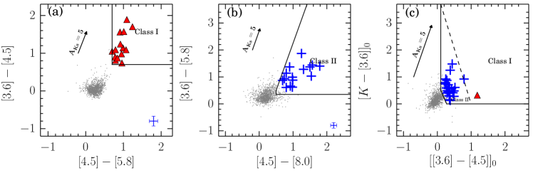
Figure 6.— Color-color diagrams used for identification of Class I and Class II YSOs. “Red Triangle” represents Class I YSOs and “Blue Plus” denotes Class II YSOs, “Filled gray circle” represents field stars. The arrows show an extinction vector of $A_{K}=5$ mag.

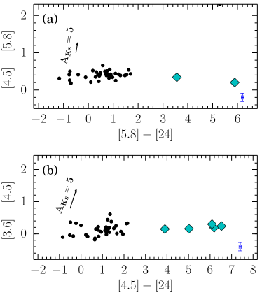
Figure 7.— Color-color diagrams used for identification of additional transition disks. “Cyan Diamonds” represent the transition disk YSOs, “Filled black circles” represent field stars. The arrows show an extinction vector of $A_{K}=5$ mag.

Infrared colors as a powerful proxy for measuring the excessive emission have been demonstrated by many authors (e.g., Allen et al. (2004); Gutermuth et al. (2008)). Using the color selection scheme of Gutermuth et al. (2009), we identify YSOs associated with the bubble in the light of Spitzer and UKIDSS data. The feasibility of this scheme has been demonstrated in many star-forming regions located at different distances, such as W5-east NGC7538 (Chavarría et al., 2014) and NGC6634 (Willis et al., 2013). The procedure of isolating YSOs were carried out as below:

1. We picked out 1239 sources having photometric uncertainties $\sigma<0.2$ mag detections in all four IRAC bands. To ensure a confident YSO sample, 2 star-forming galaxies, 1 broad-line AGN, 1 knot of shock emission and 331 sources with PAH-contaminated apertures were removed by the criteria in various color spaces (Gutermuth et al., 2009). The remaining uncontaminated sources are considered to be Class I YSOs, if their colors follow: (1) $[4.5]-[5.8]>0.7$, and (2) $[3.6]-[4.5]>0.7$; and Class II YSOs, if their colors follow: (1) $[4.5]-[8.0]-\sigma_{24}>0.5$, (2) $[3.6]-[5.8]-\sigma_{13}>0.35$, (3) $[3.6]-[5.8]+\sigma_{13}\leq\frac{0.14}{0.04}\times(([4.5]-[8.0]-\sigma_{24})-0.5)+0.5$, and (4) $[3.6]-[4.5]-\sigma_{12}>0.35$, where $\sigma_{24},\sigma_{13},\sigma_{12}$ are the combined measurement errors of two corresponding IRAC bands (i.e., [4.5] and [5.8], [3.6] and [4.5], [3.6] and [4.5], respectively). In the end, 14 Class I and 15 Class II YSOs are obtained by above constraints. These constraints are also shown in Fig. 6a and Fig. 6b.

2. There are 8281 sources lacking detections at either 5.8 or 8.0 $\mu$m. We selected 2005 sources with $\sigma<0.2$ mag detections at both 3.6 $\mu$m and 4.5 $\mu$m and with $\sigma<0.1$ mag detections at least in UKIDSS near-infrared $H$ and $Ks$ bands. As suggested by Gutermuth et al. (2009), the line of sight extinctions of sources with only $H$ and $Ks$ bands detections are parameterized by the $E_{H-K}$ color excess, and sources with all UKIDSS bands detections are parameterized with the $\frac{E_{J-H}}{E_{H-K}}$ color excess ratio. We then computed the adopted intrinsic colors from the measured photometries, including $[J-H]_{0}$, $[H-K]_{0}$, $[K-[3.6]]_{0}$ and $[[3.6]-[4.5]]_{0}$. Based on these dereddended colors, we identified additional YSOs candidates following constraints: (1) $[[3.6]-[4.5]]_{0}-\sigma_{12}>0.101$ (2) $[K-[3.6]]_{0}-\sigma_{K1}>0$, and (3) $[K-[3.6]]_{0}-\sigma_{K1}>-2.85714\times([[3.6]-[4.5]]_{0}-\sigma_{12}-0.101)+0.5$ where $\sigma_{K1}$ is the combined measurement error of $K$ and $[3.6]$. After further investigation, we found sources that obey $[K-[3.6]]_{0}-\sigma_{K1}>-2.85714\times([[3.6]-[4.5]]_{0}-\sigma_{12}-0.401)+1.7$ are likely protostars and Class II YSOs, with the difference that Class II sources follow $[3.6]_{0}<14.5$, while all protostars obey $[3.6]_{0}<15$. With this method, we obtain 1 Class I and 27 Class II YSOs. The corresponding constraints are displayed in Fig. 6c.

3. Combing objects with MIPS 24 $\mu$m detections with $\sigma<0.2$ mag, we isolated another 5 YSOs. They are transition disk sources, and classified as sources in an evolutionary stage between Class II and Class III (Gutermuth et al., 2009). They obey all the following criteria: (1) $[24]<7$, (2) $[5.8]-[24]>2.5$ or $[4.5]-[24]>2.5$, (3) $[3.6]<14$. Figure 7 displays the corresponding criteria applied to the data.

As the result of the schemes described above, 62 YSO candidates were obtained. Combing them with 8 and 24 $\mu$m images, we found two compact sources not identified as YSO candidates but are bright in the both 8 and 24 $\mu$m image. One possible reason is that they are devoid of point-source photometries at longer wavelengths in IRAC bands due to the diffuse emission. One of them, G024.1754+00.3994, is confirmed to be a compact HII region (see Sect. 5.3). The other one, residing in the north of G24.136, is considered to be a Class I protostar due to its bright emission at 24 $\mu$m.

We note that some true YSOs might not be isolated since they reside in bright backgrounds (i.e., bright PAH emission), suggesting that the present number of YSO candidates may be a lower limit. The SED fitting to all point sources with detections in at least three wavelength bands (Liu et al., 2014, in preparation) would select more YSO candidates. Table 4 gives a summary of 63 YSO candidates (17 Class I, 42 Class II and 5 transition disk). Figure 4 displays their spatial distributions overlaid on the ¹²CO (1-0) and ¹³CO (1-0) velocity-integrated intensities. The majority of the YSO candidates projected on the region with moderate molecular gas indicates active star formation surrounding G24.136.

Figure 8.— Result of the fit to the candidate of exciting star using the on-line SED fitting tool of Robitaille et al. (2006). The filled circles show the input fluxes, and the black line shows the best fit stellar photosphere model.

5. Discussion

Table 3Observed Parameters of IRAS Sources

Name	R.A.	DEC.	$err_{rmaj}^{a}$	$err_{rmin}^{a}$	$err_{PA}^{a}$	$F_{12}$	$F_{25}$	$F_{60}$	$F_{100}$	$f_{qual}^{b}$	$log(\frac{F_{25}}{F_{12}})$	$log(\frac{F_{60}}{F_{12}})$	$L_{IR}^{c}$
	(h m s)	(d m s)	(arcsec)	(arcsec)	(deg)	(Jy)	(Jy)	(Jy)	(Jy)				($10^{4}L_{\odot}$)
18308-0741	18:33:35.859	-7:38:51.35	8	22	86	4.145	7.804	166.6	560.2	3232	0.27	1.60	1.8
18312-0738	18:33:57.318	-7:36:11.75	6	56	85	1.802	4.806	72.56	396.1	2332	0.43	1.60	1.0

5.1. Star Formation Scenarios in Cores

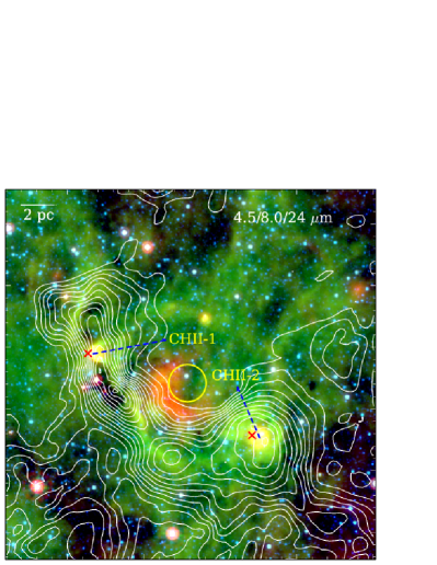
Figure 9.— Three-color composite image in 4.5 $\mu$m (blue), 8.0 $\mu$m (green) and 24 $\mu$m (red). Two compact HII regions are labeled as CHII-1 and CHII-2. The yellow circle represents a possible zone of existing ionizing sources. The white contours and other symbols are the same as those in Fig. 4. In the center of the bubble, the 24 $\mu$m cavity is considered to be hot dust broken by stellar winds. A scale bar of 2 pc is shown on the top left.

The consistence of YSOs’ spatial distribution with CO emission suggests that recently formed stars form within the molecular cloud and that star formation around the bubble is active. Additionally, the good match of dense molecular gas with PAH emission from PDRs and 24 $\mu$m emission from hot dust regions demonstrates the strong influence of IF created by the HII region on its surroundings. Star formation around the bubble has to be affected by the expanding HII region. In what follows, we will discuss the star formation scenarios associated dense cores, coupled with their physical properties.

Core A is located on the northeast of the bubble. Within this core, $\sim 8$ embedded YSO candidates (i.e., 1 Class I, 5 Class II, 1 transition disk, and CHII-1) show IR excess emission in MIR or NIR wavelengths. In Fig. 9, If the angular resolution was high enough, Core A would be divided into a part coincided with an IR filament structure along the NW-SE direction and the other part enclosing CHII-1 in the edge of the bubble. Along the major axis of Core A (i.e., the direction NE-SW), emission of molecular gas of the core shows the steep increase of intensities in the outskirts. In Fig. 9, some evolved stars and YSOs possibly associated with this core are located in the front of it. Therefore, the large gradient of intensity of ¹³CO (1-0) may be partially as a result of the external compression from them. It is plausible to partially attribute the broad line-width of ¹³CO (1-0) in Core A, $3.92\pm 0.16$ km s^-1, to the external pressure. Another star formation activities are also responsible for the broad line-width. One IRAS source, 18312-0738, offsetting $45\arcsec$ from the peak of both Core A and CHII-1, is associated with the core. We note that this offsetting may result from a poor IRAS positoin accuracy of $30\arcsec$. Following Casoli et al. (1986), the observed fluxes at 12, 25, 60 and 100 $\mu$m indicate an infrared luminosity $L_{\mathrm{IR}}$ of $\sim 2\times 10^{4}$ $L_{\odot}$ (see Table 3), demonstrating a massive stellar system. This is in great agreement with the existence of CHII-1. And hence, activities of massive star formation do proceed in Core A, causing strong non-thermal motions and leading to the core, to some extent, with the broad line-width of ¹³CO (1-0).

Core B is located on the east of the bubble. Five embedded YSO candidates (three Class I and two Class II) within the core are indicative of presence of active star formation in Core B. They may disturb their surrounding environments, broadening the measured line-width of spectra. Thus, the broad line width of Core B, $\sim 4.94$ km s^-1, could be partly attributed to the non-thermal motions driven by powerful activities of star formation. In addition, the high LTE mass (a few of $10^{3}$ $M_{\odot}$) and intermediate number density (a few of $10^{3}$ cm^-3) of Core B show a probability of forming a low-mass cluster or even high-mass protostars, which could also be supported by the existence of two bright 24 $\mu$m point sources embedded within the core. Figure 9 shows that the IR counterpart of Core B is seen in absorption in both 8 $\mu$m and 24 $\mu$m against the infrared background. This indicates that molecular gas is located in front of the IR emission, which is well consistent with the fact that this IR counterpart is an infrared dark cloud (IRDC) (Peretto & Fuller, 2009). The association of IRDC with Core B along with no detectable enclosed HII regions indicates that it is younger than Core A.

Core C is located on the south periphery of the bubble. Around six YSO candidates (two Class I and four Class II) are associated with the core. This shows the history of active ongoing star formation. The strong activities of star formation coupled with the effects of the HII region on the Core C could produce non-thermal motions, resulting in the present broad line-width of ¹³CO (1-0), $\sim 6$ km s^-1. In Comparison with Core B, there are no YSOs close to the emission peak of Core C, therefore, we suggest that Core C may be younger than Core B.

Core D is located on the southwest of the bubble. One embedded Class II YSO candidate offsets from the peak of the molecular core. We note that some true YSOs may be missed due to the limitation of the color-color scheme aforementioned in Sect. 4.3. The broad line width ($3.03\pm 0.16$ km s^-1), high number density ($1.3\pm 0.2\times 10^{3}$ cm^-3) and mass ($3.6\pm 0.1\times 10^{3}$ $M_{\odot}$) of Core D are comparable to those of three cores aforementioned. Given Core D not associated with either any bright 24 $\mu$m point sources or strong PDRs, it would be at an early stage or in the process or in the process of low-mass star formation.

Core E is located on the southwest of the bubble. About seven YSO (four Class I and three Class II) candidates are associated with the core. Six of them distribute sparsely in the outer edge of the core. This may be inconsistent with the actual situations due to the missing problem of identifying YSOs mentioned above. In the center of Core E, one Class I object and one bright IRAS source (i.e., 18308-0741) are detected. The IRAS source has an estimated luminosity of $\sim 10^{4}$ $L_{\odot}$. This is a good indicator of a massive stellar system, in a good agreement with the fact that CHII-2 has formed beginning to ionize the neighbor ISMs and sculpt a small photoionized bubble of gas embedded within the cold, dense, and massive molecular core (see Sect. 5.3). With energetic activities of massive star formation developing, inevitable non-thermal disturbances have to be emerged. Therefore, the broad linewidth of Core E, $\sim 2.69$ km s^-1, could be partially interpreted as broadening of the disturbances. Due to the existence of the compact ionized region in Core A and Core E, their evolved lifetimes are comparable.

Core F is located on the west of the bubble. A total of $\sim 3$ YSO candidates (two Class II and one transition disk) distribute along the edge of the core, witnessing the star formation history. It is the diffuse molecular entity with the lowest column density, number density and LTE mass among all cores. Given the core lying away from the bubble (see Fig. 9), effects of the classical HII region on Core F may be weaker than on other cores.

5.2. Exciting Stars

To investigate the main exciting star, we calculate the number of UV ionizing photons per second ($N_{\mathrm{uv}}$) from the free-free emission at 20 cm, based on the following equation (Chaisson, 1976):

$$N_{\mathrm{uv}}=0.76\times 10^{47}T_{4}^{-0.45}\nu_{\mathrm{GHz}}^{0.1}S_{\nu}d_{\mathrm{kpc}}^{2}$$ (5)

where $T_{4}$ is the electron temperature in units of $10^{4}$ K, $S_{\nu}$ is the measured flux density in units of Jy, $\nu_{\mathrm{GHz}}$ is the frequency in units of GHz and $d_{\mathrm{kpc}}$ is the distance in units of kpc. If the HII region reaches the equilibrium at an electron temperature of $T=10^{4}$ K and a total flux density of $0.46\pm 0.05$ Jy at 20 cm (measured by integrating over the $4\sigma$ ($\sigma=$0.15 mJy/beam) contour within the radius of the HII region), the estimated value of $N_{\mathrm{uv}}$ is $1.15\pm 0.04\times 10^{48}$ ph s^-1. In this calculation, any ionizing photons absorbed by dust or running away from the bubble were not accounted for, and hence, the present $N_{\mathrm{uv}}$ has been underestimated. Similar argument is made by Watson et al. (2008), on the basis of studies of several bubbles, that $N_{\mathrm{uv}}$ estimated with this method is statistically lower than the expected value by about a factor of 2. In the following, we adopt $\sim 2.3\times 10^{48}$ ph s^-1 as a reference value. It corresponds to a spectral type of $\sim$O8V (see Table 4 of Martins et al. (2005)). Given uncertainties aforementioned, the estimated spectral type should be considered with a caveat.

Following the method of searching for exciting stars (Pomarès et al., 2009), sources with all detections in NIR and IRAC bands were extracted from a region centered at the hot dust cavity seen at 24 $\mu$m (i.e., the yellow solid circle in Fig. 9). The SED fittings to these sources give one potential candidate, G024.1416+00.4364. Its result of SED fitting is displayed in Fig. 8, deriving a temperature of $\sim 3.5\times 10^{4}$ K and a mass of $\sim 20$ $M_{\odot}$. These values are consistent with stellar parameters of $\sim$O8V (Martins et al., 2005). Therefore, G0241416+00.4364 would be a major exciting star candidate which could provide enough energy to create the dust bubble and regulate its surroundings.

5.3. Two Compact HII regions

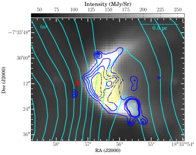
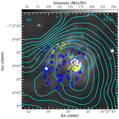
Figure 10.— (a): 8.0 $\mu$m image of the compact HII region, CHII-1, overlaid with contours of the radio continuum emission at 20 cm in yellow, 4.5 $\mu$m emission in blue, and ¹³CO (1-0) emission in cyan. The contours start from 0.9 mJy/pixel with a step of 0.2 mJy/pixel for the 20 cm emission, from 8 MJy/sr with a step of 4 MJy/sr for the 4.5 $\mu$m emission and from 19.6 K km s^-1 with a step of 0.7 K km s^-1 for the ¹³CO (1-0) intensity. The red cross represents the IRAS source 18308-0741. A scale bar of 0.5 pc is shown on the top right. (b): Same for the compact HII region, CHII-2. The contours start from 0.8 mJy/pixel with a step of 0.2 mJy/pixel for the 20 cm emission, from 8 MJy/sr to 16 MJy/sr and finally to 28 MJy/sr for the 4.5 $\mu$m emission and from 7 K km s^-1 with a step of 0.7 K km s^-1  for the ¹³CO (1-0) intensity. The red cross represents the IRAS source 18312-0738. A scale bar of 0.5 pc is shown on the top right.

Figure 9 displays the two compact sources, G024.1754+00.3994 and G024.0953+00.4579 denoted as CHII-1 and CHII-2 respectively. These two sources are clearly associated with thermal free-free continuum at 20 cm, PAH emission from the PDRs, and hot dust emission out of thermal equilibrium seen at 24 $\mu$m. In existing studies (e.g., Urquhart et al. (2013), and reference therein), these observable features have always been adopted as useful criteria to identify ultracompact (UC) or compact HII regions. They are generally of different scale sizes and particle densities: $D\leq 0.1$ pc and $n\geq 10^{4}$ cm^-3 for UCHII regions; $D\leq 0.5$ pc and $n\geq 10^{3}$ cm^-3 for CHII regions (Kurtz, 2005). The free-free emission confines the size of CHII-1 and CHII-2 to be 0.4 pc and 0.8 pc respectively. In combination of their number density of $\sim 10^{3}$ cm^-3 (assumed to be similar to those of their hosting molecular cores), they could be plausibly identified as CHII candidates. These two CHII candidates coupled with the classic HII region inside the bubble exhibit a hierarchical structure, indicative of secondary star formation on the rim of the bubble.

CHII-1 and CHII-2 have flux densities of $2.7\pm 0.3$ mJy and $8.0\pm 0.2$ mJy at 20 cm respectively. The minimum ionizing photon flux required to maintain ionization of the region is log $N_{Lyc}>45.8$ for CHII-1 and $>46.3$ for CHII-2, both corresponding to a B0.5V star (Panagia, 1973). In the two CHII sources, the 4.5 $\mu$m emission tracing shocked molecular gas (Cyganowski et al., 2008) is spatially coincided with the bright PAH emission and consistent with the free-free emission. This sheds light on the strong influence of ionizing sources on their natal molecular cloud (i.e., Core A and Core E), indicating the possibility of existing outflows from massive stars. Of greater interest is the CHII-1, as its morphology appears as a cometary object seen in both the 4.5 and 8.0 $\mu$m image. High resolution observations of these two sources would help to determine their nature and origin.

5.4. Feedback From Massive Stars

G24.136 is an almost perfectly spherical bubble around the HII region ionized by an $\sim$O8V star(s). The PDRs just outside the IF suggests that the strong influence of the HII region on its adjacent molecular cloud. This influence could be partially supported by shocked compressed material at the outskirts of the shell-like molecular cloud. In G24.136 the hot dust cavity broken along the northwest indicates that the stellar winds from an late-O star (stars) probably play a critical role in affecting its associated cloud. The feedback of stellar winds has also been proposed in the study of the bubbles N10, N21, N49 (Watson et al., 2008).

On the one hand, Deharveng et al. (2012) suggested that during the evolution of an HII region its IF reaches regions of lower density than those of higher density and the ionization occurs more quickly in the former case. In diffuse region of lower densities, no neutral material might be collected, which applies well to G24.136. The diffuse and rarified molecular gas associated with diffuse PAH emission to the northwest of G24.136 indicates the original mediums of low densities and the photoionization of the HII region. Additionally, few young stars means that star formation to the northwest of G24.136 might be halted due to disruptions of molecular gas by the expansion of the HII region and stellar winds. On the other hand, neutral material seems to be collected into the border on the southeast of G24.136. The consistence of YSOs’ spatial distribution with the collected layer shows active star formation on the border of the bubble. Additionally, the hierarchies of secondary star formation on the rim of the bubble (see Sect. 5.3) indicates a promising sign for triggering star formation (Oey et al., 2005; Zavagno et al., 2006; Deharveng et al., 2010; Elmegreen, 2011; Simpson et al., 2012; Samal et al., 2014).

5.5. Collect and Collapse Process

The morphology of the cloud projected on the periphery of G24.136 indicates that the shocked molecular layer is presumably swept up and assembled during the bubble’s expansion, whereby we discuss star formation within the bubble in the context of the collect and collapse process.

The dynamical age of the HII region can be simply estimated as follows (Dyson & Williams, 1980):

$$R_{s} = (3N_{\mathrm{uv}}/4\pi n_{0}^{2}\alpha_{B})^{1/3}$$

$$t_{\mathrm{dyn}} = (\frac{4R_{s}}{7c_{s}})[(\frac{R}{R_{s}})^{7/4}-1]$$ (6)

where $R_{s}$ is the radius of the Stromgren sphere in units of cm, $n_{0}$ is the initial particle density of ambient neutral gas in units of cm^-3, $\alpha_{B}$ = $2.6\times 10^{-13}(10^{4}\mathrm{K}/T)^{0.7}$ cm³ s^-1 (Kwan, 1997) is the the coefficient of the radiative recombination, c_s is the isothermal sound speed of ionized gas assumed to be 10 km s^-1, $R$ is the radius of the HII region in units of cm. To obtain an approximate $n_{0}$, we assume that the total mass of the molecular shell (i.e., $2\times 10^{4}$ $M_{\odot}$) was distributed homogeneously in a sphere of radius 3.9 pc (i.e., the bubble radius), which gives an estimated density of $\sim 1.3\times 10^{3}$ cm^-3. This value may be just a lower limit since this estimate does not consider the mass of the ionized gas within the bubble. Therefore, we adopt the average density over the six cores (i.e., $\sim 1.6\times 10^{3}$ cm^-3) as a possible upper limit. If G24.136 formed and evolved in a uniform density of $(1.3-1.6)\times 10^{3}$ cm^-3, the bubble’s radius of $3.7\pm 0.7$ pc derives dynamical ages of $1.5-1.6$ Myr. We note that the the realistic evolution of the HII region is not in a strictly uniform medium, therefore, the estimated age is very uncertain, and should be considered with a caution.

The analytical model of Whitworth et al. (1994) describes fragmentation time of the shocked dense layer surrounding expanding HII regions. The time at which the fragmentation commences is calculated as follows:

$$t_{\mathrm{frag}}=1.56a_{.2}{}^{7/11}N_{49}{}^{-1/11}n_{3}{}^{-5/11}$$ (7)

where $a_{0.2}$ is the sound speed inside the shocked layer in unites of 0.2 km s^-1, $N_{49}$ is the ionizing photon flux in units of $10^{49}$ ph $s^{-1}$, and $n_{3}$ is the initial gas atomic number density in units of $10^{3}$ cm^-3. The above calculation shows $t_{frag}$ depends weakly on $N_{uv}$, somewhat on $n_{0}$ and greatly on $a_{s}$. We consider the thermal sound speed in the collected layer to be $\sim 0.2$ km s^-1at an average temperature of $\sim 16$ K over the shell, indicating fragmentation time of $\sim 1.7$ Myr for the density of $\sim 1.3\times 10^{3}$ cm^-3 and $\sim 1.5$ Myr for the density of $\sim 1.6\times 10^{3}$ respectively. In the estimate of fragmentation time, the stellar winds have not been took into account due to lacking their mechanical luminosity. Therefore, fragmentation time derived from Eq. 7 is overestimated. Given the uncertainty, this time scale is comparable to or even smaller than the dynamical age of the HII region. This demonstrates that during the lifetime of G24.136 the collected molecular cloud has enough time to become gravitationally unstable to fragment into molecular cores. This process follows the model of “collect and collapse”, which is indicative of triggering.

To conclude, a combination of the enhanced number of candidate YSOs as well as secondary star formation in the collected layer and time scales involved ($t_{\mathrm{dyn}},t_{\mathrm{frag}}$) indicates a possible scenario of triggered star formation towards G24.136 by both the expansion of the bubble and stellar winds, signified by the “collect and collapse” process.

While the conclusion on triggering in G24.136 is conservative, it remains to be further confirmed because of at least three difficulties. First, it is hard to discern which stars are triggered and which stars formed spontaneously (Elmegreen, 2011; Dale & Bonnell, 2011; Dale et al., 2012, 2013). Second, the YSOs surface density enhancement on the rim of the bubble might be re-distributed by its expansion or forming in situ (Elmegreen, 2011). Finally, the incompleteness of YSO candidates aforementioned in Sect. 4.3 hardly restore their true spatial distribution. All these problems hinder us from giving any convincing evidence on triggering. In later work of Liu et al. (2014, in preparation), we will run SED fitting to 10509 sources to select more completed YSO candidates. Analyzing their age differences (in an attempt to search for possible age gradients) would be useful to remit above difficulties.

6. Summary

We have performed an extensive study of the IR bubble G24.136 using J=1-0 lines of CO and its isotopologues, infrared and radio data. The main results are summarized as follows:

1. The molecular gas around the bubble has a velocity of $94.8\pm 0.42$ km s^-1. Its emission is prominently in the southeast of the bubble, sculpted as a shell with a mass of $\sim 2\times 10^{3}$ $M_{\odot}$. It is presumably assembled during the expansion of the bubble.

2. The expanding shell consists of six dense cores. Their dense (a few of $10^{3}$ cm^-3) and massive (a few of $10^{3}$ $M_{\odot}$) properties coupled with the broad linewidths ($>2.5$ km s^-1) suggest they are promising sites of forming high-mass stars or clusters. This, in fact, could be further consolidated by the two compact HII regions embedded within Core A and Core E.

3. We tentatively identified and classified 63 YSO candidates (16 Class I, 42 Class II and 5 Transition-disk objects) by the color scheme. They are predominantly projected on the regions with strong emission of molecular gas, showing active star formation especially in the shell.

4. G24.136 surrounds an almost spherical HII region. It is ionized by an $\sim$O8V star(s), of the dynamical age $\sim$1.6 Myr. The PDRs just outside the IF and the dust cavity demonstrate the strong influence of both HII region and stellar winds on the adjacent environments and star formation.

5. From the enhanced number of YSO candidates and secondary star formation in the shell, we suggest that star formation in the shell might be triggered by a combination of the expanding HII region and stellar winds. The comparison between the estimated dynamical age of the HII region and the fragmentation time of the shell further indicates that triggered star formation might function through the “collect and collapse” process.

Table 4Results of YSO Classification.

Number	Designation	R.A.	DEC.	$J$	$H$	$K$	$3.6$	$4.5$	$5.8$	$8.0$	$24$	Type	Associations†
		(deg)	(deg)	(mag)	(mag)	(mag)	(mag)	(mag)	(mag)	(mag)	(mag)
1	G024.1244+00.5352	18h33m21.316s	-7d35m07.46s	14.55 ( 0.05)	12.18 (0.05)	10.97 ( 0.03)	9.88 ( 0.03)	9.68 ( 0.03)	9.26 ( 0.03)	8.70 ( 0.02)	6.99 ( 0.02)	II	F
2	G024.0286+00.4726	18h33m24.076s	-7d41m57.63s	nan ( nan)	nan ( nan)	nan ( nan)	12.42 ( 0.06)	11.94 ( 0.09)	11.43 ( 0.09)	10.95 ( 0.11)	nan ( nan)	II
3	G024.0233+00.4617	18h33m25.823s	-7d42m32.63s	15.60 ( 0.09)	14.29 (0.08)	13.48 ( 0.06)	12.70 ( 0.09)	12.28 ( 0.09)	nan ( nan)	nan ( nan)	nan ( nan)	II
4	G024.0219+00.4606	18h33m25.902s	-7d42m38.76s	nan ( nan)	nan ( nan)	nan ( nan)	14.41 ( 0.14)	12.86 ( 0.10)	11.95 ( 0.14)	nan ( nan)	nan ( nan)	I
5	G024.0612+00.4757	18h33m27.045s	-7d40m08.33s	nan ( nan)	nan ( nan)	13.09 ( 0.05)	10.54 ( 0.04)	9.56 ( 0.04)	8.62 ( 0.03)	7.71 ( 0.02)	5.93 ( 0.02)	I	E
6	G024.1028+00.4953	18h33m27.489s	-7d37m22.84s	nan ( nan)	14.41 (0.07)	13.73 ( 0.08)	13.10 ( 0.06)	12.75 ( 0.09)	nan ( nan)	nan ( nan)	nan ( nan)	II	E
7	G024.1361+00.5104	18h33m27.956s	-7d35m11.34s	nan ( nan)	nan ( nan)	nan ( nan)	13.27 ( 0.06)	13.09 ( 0.08)	nan ( nan)	nan ( nan)	6.89 ( 0.04)	TD	F
8	G024.1102+00.4905	18h33m29.328s	-7d37m07.17s	nan ( nan)	14.49 (0.06)	13.21 ( 0.04)	12.27 ( 0.06)	11.74 ( 0.08)	11.74 ( 0.12)	nan ( nan)	nan ( nan)	II	E
9	G024.0696+00.4656	18h33m30.166s	-7d39m58.15s	nan ( nan)	nan ( nan)	nan ( nan)	10.51 ( 0.03)	9.61 ( 0.03)	8.84 ( 0.03)	9.06 ( 0.03)	nan ( nan)	I	E
10	G024.1283+00.4927	18h33m30.869s	-7d36m05.78s	13.66 ( 0.03)	13.10 (0.03)	12.65 ( 0.03)	12.01 ( 0.07)	11.82 ( 0.07)	11.59 ( 0.11)	nan ( nan)	nan ( nan)	II	F
11	G024.0531+00.4496	18h33m31.747s	-7d41m17.57s	14.83 ( 0.04)	14.30 (0.04)	13.99 ( 0.08)	13.77 ( 0.07)	12.61 ( 0.11)	nan ( nan)	nan ( nan)	nan ( nan)	I	E
12	G024.1231+00.4796	18h33m33.125s	-7d36m43.97s	13.54 ( 0.03)	10.08 (0.02)	8.20 ( 0.03)	6.71 ( 0.03)	6.32 ( 0.03)	5.78 ( 0.02)	5.58 ( 0.02)	4.92 ( 0.01)	II	E
13	G024.1689+00.5021	18h33m33.396s	-7d33m40.50s	nan ( nan)	nan ( nan)	nan ( nan)	13.88 ( 0.10)	12.78 ( 0.08)	11.71 ( 0.10)	11.80 ( 0.14)	8.32 ( 0.03)	I
14	G024.0953+00.4579	18h33m34.670s	-7d38m49.04s	15.70 ( 0.08)	12.72 (0.06)	10.67 ( 0.03)	8.54 ( 0.09)	7.81 ( 0.05)	6.84 ( 0.06)	6.08 ( 0.14)	nan ( nan)	I	E
15	G024.1554+00.4863	18h33m35.286s	-7d34m49.72s	14.73 ( 0.06)	13.90 (0.08)	13.29 ( 0.06)	12.85 ( 0.05)	12.52 ( 0.07)	12.31 ( 0.18)	nan ( nan)	nan ( nan)	II
16	G024.0378+00.4081	18h33m38.959s	-7d43m15.37s	14.78 ( 0.04)	14.16 (0.05)	13.79 ( 0.07)	13.56 ( 0.09)	13.23 ( 0.08)	nan ( nan)	nan ( nan)	nan ( nan)	II
17	G024.1022+00.4304	18h33m41.361s	-7d39m12.69s	nan ( nan)	nan ( nan)	nan ( nan)	11.84 ( 0.04)	11.48 ( 0.06)	10.96 ( 0.07)	10.50 ( 0.18)	nan ( nan)	II	D
18	G024.1629+00.4584*	18h33m42.121s	-7d35m12.10s	nan ( nan)	nan ( nan)	nan ( nan)	13.94 ( 0.09)	13.55 ( 0.16)	nan ( nan)	nan ( nan)	nan ( nan)	I
19	G024.2168+00.4853	18h33m42.363s	-7d31m35.32s	14.18 ( 0.04)	13.59 (0.05)	13.29 ( 0.05)	12.95 ( 0.06)	12.60 ( 0.12)	nan ( nan)	nan ( nan)	nan ( nan)	II
20	G024.0813+00.4141	18h33m42.514s	-7d40m46.32s	nan ( nan)	nan ( nan)	13.61 ( 0.04)	12.18 ( 0.05)	11.91 ( 0.05)	11.51 ( 0.08)	10.99 ( 0.17)	nan ( nan)	II	C
21	G024.1080+00.4241	18h33m43.353s	-7d39m04.48s	15.25 ( 0.05)	14.47 (0.05)	13.64 ( 0.07)	12.29 ( 0.05)	11.89 ( 0.07)	11.77 ( 0.09)	nan ( nan)	nan ( nan)	II	C
22	G024.1121+00.4182	18h33m45.088s	-7d39m01.28s	nan ( nan)	nan ( nan)	nan ( nan)	13.73 ( 0.07)	11.84 ( 0.07)	10.75 ( 0.06)	10.71 ( 0.15)	6.39 ( 0.02)	I	C
23	G024.0695+00.3902	18h33m46.342s	-7d42m03.70s	10.75 ( 0.03)	7.99 (0.04)	6.35 ( 0.02)	5.36 ( 0.16)	4.79 ( 0.04)	4.22 ( 0.03)	3.99 ( 0.06)	1.69 ( 0.03)	II
24	G024.1304+00.4180	18h33m47.169s	-7d38m03.09s	nan ( nan)	nan ( nan)	nan ( nan)	12.53 ( 0.08)	11.66 ( 0.06)	10.82 ( 0.07)	10.45 ( 0.06)	nan ( nan)	I	C
25	G024.1650+00.4325	18h33m47.911s	-7d35m48.33s	15.02 ( 0.06)	14.13 (0.07)	13.71 ( 0.07)	12.90 ( 0.07)	12.65 ( 0.09)	nan ( nan)	nan ( nan)	nan ( nan)	II
26	G024.1882+00.4411	18h33m48.660s	-7d34m20.25s	nan ( nan)	14.72 (0.06)	13.95 ( 0.06)	12.90 ( 0.06)	12.57 ( 0.08)	12.44 ( 0.17)	nan ( nan)	nan ( nan)	II
27	G024.1192+00.4014	18h33m49.492s	-7d39m06.45s	15.45 ( 0.06)	13.99 (0.07)	13.29 ( 0.06)	12.85 ( 0.06)	12.38 ( 0.08)	nan ( nan)	nan ( nan)	nan ( nan)	II	C
28	G024.2132+00.4498	18h33m49.584s	-7d32m45.81s	nan ( nan)	12.48 (0.03)	9.98 ( 0.02)	6.83 ( 0.04)	5.75 ( 0.04)	4.96 ( 0.02)	4.30 ( 0.02)	2.44 ( 0.03)	I
29	G024.0762+00.3783	18h33m49.650s	-7d42m02.08s	15.16 ( 0.05)	14.36 (0.06)	13.89 ( 0.07)	13.48 ( 0.11)	13.01 ( 0.12)	nan ( nan)	nan ( nan)	nan ( nan)	II
30	G024.1183+00.3868	18h33m52.529s	-7d39m33.46s	nan ( nan)	12.89 (0.03)	10.12 ( 0.03)	7.91 ( 0.03)	7.67 ( 0.03)	7.29 ( 0.02)	6.87 ( 0.02)	6.76 ( 0.01)	II	C
31	G024.1902+00.4231	18h33m52.755s	-7d34m43.65s	nan ( nan)	nan ( nan)	nan ( nan)	11.94 ( 0.03)	11.29 ( 0.04)	10.66 ( 0.06)	9.98 ( 0.06)	8.31 ( 0.05)	II	B
32	G024.0772+00.3604	18h33m53.598s	-7d42m28.52s	13.78 ( 0.04)	13.20 (0.06)	12.65 ( 0.06)	12.09 ( 0.08)	11.81 ( 0.06)	11.72 ( 0.12)	nan ( nan)	nan ( nan)	II
33	G024.1165+00.3794	18h33m53.911s	-7d39m51.58s	14.87 ( 0.06)	14.11 (0.09)	13.60 ( 0.07)	13.24 ( 0.07)	12.88 ( 0.12)	nan ( nan)	nan ( nan)	nan ( nan)	II
34	G024.1193+00.3801	18h33m54.066s	-7d39m41.49s	13.04 ( 0.03)	12.63 (0.04)	12.32 ( 0.05)	12.34 ( 0.06)	12.03 ( 0.07)	11.77 ( 0.09)	nan ( nan)	nan ( nan)	II
35	G024.0851+00.3603	18h33m54.500s	-7d42m03.45s	nan ( nan)	14.73 (0.08)	14.06 ( 0.09)	12.80 ( 0.08)	12.41 ( 0.11)	nan ( nan)	nan ( nan)	nan ( nan)	II
36	G024.1562+00.3942	18h33m55.162s	-7d37m19.97s	nan ( nan)	nan ( nan)	nan ( nan)	13.65 ( 0.07)	12.08 ( 0.06)	11.07 ( 0.06)	nan ( nan)	nan ( nan)	I
37	G024.1569+00.3938	18h33m55.340s	-7d37m18.47s	nan ( nan)	nan ( nan)	nan ( nan)	13.76 ( 0.07)	12.05 ( 0.06)	10.82 ( 0.06)	10.12 ( 0.04)	nan ( nan)	I	B
38	G024.0843+00.3545	18h33m55.662s	-7d42m15.79s	nan ( nan)	nan ( nan)	nan ( nan)	13.30 ( 0.09)	12.49 ( 0.06)	11.71 ( 0.11)	11.17 ( 0.08)	nan ( nan)	I
39	G024.2214+00.4257	18h33m55.668s	-7d32m59.47s	15.61 ( 0.07)	14.25 (0.10)	13.49 ( 0.08)	12.68 ( 0.06)	12.52 ( 0.13)	nan ( nan)	nan ( nan)	7.50 ( 0.03)	TD	A
40	G024.1622+00.3921	18h33m56.276s	-7d37m04.33s	nan ( nan)	12.79 (0.07)	10.53 ( 0.03)	8.02 ( 0.08)	6.97 ( 0.06)	6.27 ( 0.03)	5.56 ( 0.02)	3.57 ( 0.03)	I	B
41	G024.2018+00.4077	18h33m57.350s	-7d34m31.98s	nan ( nan)	nan ( nan)	nan ( nan)	13.66 ( 0.07)	12.52 ( 0.09)	11.53 ( 0.11)	nan ( nan)	nan ( nan)	I	A
42	G024.2060+00.4094	18h33m57.463s	-7d34m15.70s	nan ( nan)	13.66 (0.07)	13.37 ( 0.05)	13.03 ( 0.05)	12.40 ( 0.10)	nan ( nan)	nan ( nan)	nan ( nan)	II	A
43	G024.1613+00.3859	18h33m57.501s	-7d37m17.68s	nan ( nan)	nan ( nan)	nan ( nan)	11.51 ( 0.04)	10.33 ( 0.04)	9.64 ( 0.05)	9.08 ( 0.05)	nan ( nan)	II
44	G024.1619+00.3842	18h33m57.954s	-7d37m18.64s	nan ( nan)	nan ( nan)	13.43 ( 0.05)	10.64 ( 0.03)	9.40 ( 0.03)	8.48 ( 0.03)	7.74 ( 0.02)	4.62 ( 0.02)	I	B
45	G024.2459+00.4271	18h33m58.110s	-7d31m39.03s	14.70 ( 0.04)	13.95 (0.08)	13.51 ( 0.07)	13.12 ( 0.06)	12.84 ( 0.10)	nan ( nan)	nan ( nan)	nan ( nan)	II
46	G024.1232+00.3631	18h33m58.155s	-7d39m57.12s	12.66 ( 0.03)	12.29 (0.05)	11.95 ( 0.05)	11.85 ( 0.05)	11.55 ( 0.07)	11.55 ( 0.11)	nan ( nan)	nan ( nan)	II
47	G024.1268+00.3648	18h33m58.194s	-7d39m42.85s	14.78 ( 0.07)	13.92 (0.05)	13.40 ( 0.06)	12.59 ( 0.06)	12.34 ( 0.09)	nan ( nan)	nan ( nan)	nan ( nan)	II
48	G024.1722+00.3867	18h33m58.556s	-7d36m41.38s	nan ( nan)	nan ( nan)	nan ( nan)	13.39 ( 0.07)	13.15 ( 0.13)	nan ( nan)	nan ( nan)	6.62 ( 0.05)	TD	A
49	G024.2302+00.4136	18h33m59.243s	-7d32m51.42s	13.78 ( 0.04)	10.43 (0.04)	8.61 ( 0.03)	7.25 ( 0.04)	6.91 ( 0.04)	6.38 ( 0.02)	6.23 ( 0.02)	5.17 ( 0.03)	II
50	G024.2098+00.3982	18h34m00.285s	-7d34m22.28s	nan ( nan)	12.70 (0.06)	10.79 ( 0.03)	8.67 ( 0.02)	7.94 ( 0.03)	7.30 ( 0.02)	6.43 ( 0.02)	4.10 ( 0.02)	II	A
51	G024.1685+00.3761	18h34m00.434s	-7d37m10.86s	nan ( nan)	13.94 (0.08)	12.58 ( 0.06)	10.66 ( 0.04)	9.82 ( 0.04)	9.29 ( 0.03)	8.92 ( 0.02)	7.23 ( 0.03)	II	B
52	G024.1168+00.3451	18h34m01.326s	-7d40m47.36s	13.18 ( 0.03)	12.49 (0.03)	12.16 ( 0.03)	11.91 ( 0.05)	11.76 ( 0.06)	11.42 ( 0.09)	10.81 ( 0.06)	7.86 ( 0.02)	TD	A
53	G024.2221+00.3988	18h34m01.528s	-7d33m42.03s	nan ( nan)	nan ( nan)	nan ( nan)	12.39 ( 0.05)	12.09 ( 0.07)	11.89 ( 0.11)	nan ( nan)	6.00 ( 0.04)	TD	A
54	G024.0946+00.3326	18h34m01.532s	-7d42m19.10s	14.70 ( 0.05)	14.00 (0.06)	13.49 ( 0.07)	12.97 ( 0.07)	12.71 ( 0.08)	nan ( nan)	nan ( nan)	nan ( nan)	II
55	G024.1530+00.3596	18h34m02.245s	-7d38m27.84s	12.66 ( 0.03)	12.19 (0.04)	11.85 ( 0.04)	11.52 ( 0.08)	11.06 ( 0.07)	11.37 ( 0.15)	nan ( nan)	nan ( nan)	II
56	G024.1220+00.3357	18h34m03.914s	-7d40m46.57s	nan ( nan)	nan ( nan)	13.85 ( 0.10)	12.10 ( 0.08)	11.59 ( 0.12)	11.07 ( 0.16)	10.04 ( 0.14)	nan ( nan)	II
57	G024.1343+00.3389	18h34m04.593s	-7d40m01.80s	13.88 ( 0.03)	13.14 (0.04)	12.77 ( 0.04)	12.16 ( 0.08)	11.64 ( 0.10)	nan ( nan)	nan ( nan)	nan ( nan)	II
58	G024.1006+00.3190	18h34m05.118s	-7d42m22.58s	15.25 ( 0.05)	14.55 (0.07)	13.88 ( 0.08)	13.08 ( 0.08)	12.86 ( 0.10)	nan ( nan)	nan ( nan)	nan ( nan)	II
59	G024.1393+00.3376	18h34m05.448s	-7d39m47.95s	nan ( nan)	14.56 (0.09)	13.13 ( 0.06)	12.42 ( 0.09)	11.81 ( 0.05)	11.83 ( 0.18)	nan ( nan)	nan ( nan)	II
60	G024.1441+00.3350	18h34m06.527s	-7d39m37.15s	nan ( nan)	13.71 (0.07)	13.42 ( 0.06)	13.17 ( 0.08)	12.90 ( 0.08)	nan ( nan)	nan ( nan)	nan ( nan)	II
61	G024.1581+00.3381	18h34m07.433s	-7d38m47.10s	nan ( nan)	nan ( nan)	nan ( nan)	11.76 ( 0.10)	10.91 ( 0.07)	10.36 ( 0.06)	9.12 ( 0.03)	nan ( nan)	II
62	G024.1740+00.3446	18h34m07.803s	-7d37m45.61s	nan ( nan)	nan ( nan)	nan ( nan)	13.04 ( 0.10)	12.35 ( 0.08)	11.60 ( 0.10)	10.77 ( 0.06)	nan ( nan)	II
63	G024.1981+00.3570	18h34m07.830s	-7d36m07.78s	14.75 ( 0.04)	14.17 (0.06)	13.94 ( 0.08)	13.49 ( 0.08)	13.20 ( 0.12)	nan ( nan)	nan ( nan)	nan ( nan)	II

References

- Allen et al. (2004) Allen, L. E., Calvet, N., D’Alessio, P., et al. 2004, ApJS, 154, 363
- Anderson et al. (2009) Anderson, L. D., Bania, T. M., Jackson, J. M., et al. 2009, ApJS, 181, 255
- Anderson et al. (2012) Anderson, L. D., Zavagno, A., Deharveng, L., et al. 2012, A&A, 542, A10
- Arikawa et al. (1999) Arikawa, Y., Tatematsu, K., Sekimoto, Y., & Takahashi, T. 1999, PASJ, 51, L7
- Benjamin et al. (2003) Benjamin, R. A., Churchwell, E., Babler, B. L., et al. 2003, PASP, 115, 953
- Brand & Blitz (1993) Brand, J., & Blitz, L. 1993, A&A, 275, 67
- Brand et al. (2011) Brand, J., Massi, F., Zavagno, A., Deharveng, L., & Lefloch, B. 2011, A&A, 527, A62
- Casoli et al. (1986) Casoli, F., Combes, F., Dupraz, C., Gerin, M., & Boulanger, F. 1986, A&A, 169, 281
- Chaisson (1976) Chaisson, E. J. 1976, Frontiers of Astrophysics, 259
- Chavarría et al. (2014) Chavarría, L., Allen, L., Brunt, C., et al. 2014, MNRAS, 439, 3719
- Churchwell et al. (2006) Churchwell, E., Povich, M. S., Allen, D., et al. 2006, ApJ, 649, 759
- Churchwell et al. (2009) Churchwell, E., Babler, B. L., Meade, M. R., et al. 2009, PASP, 121, 213
- Cyganowski et al. (2008) Cyganowski, C. J., Whitney, B. A., Holden, E., et al. 2008, AJ, 136, 2391
- Dale & Bonnell (2011) Dale, J. E., & Bonnell, I. 2011, MNRAS, 414, 321
- Dale et al. (2007) Dale, J. E., Bonnell, I. A., & Whitworth, A. P. 2007, MNRAS, 375, 1291
- Dale et al. (2013) Dale, J. E., Ercolano, B., & Bonnell, I. A. 2013, MNRAS, 431, 1062
- Dale et al. (2012) Dale, J. E., Ercolano, B., & Bonnell, I. A. 2012, MNRAS, 427, 2852
- Deharveng et al. (2008) Deharveng, L., Lefloch, B., Kurtz, S., et al. 2008, A&A, 482, 585
- Deharveng et al. (2010) Deharveng, L., Schuller, F., Anderson, L. D., et al. 2010, A&A, 523, A6
- Deharveng et al. (2005) Deharveng, L., Zavagno, A., & Caplan, J. 2005, A&A, 433, 565
- Deharveng et al. (2012) Deharveng, L., Zavagno, A., Anderson, L. D., et al. 2012, A&A, 546, A74
- Denoyer (1979) Denoyer, L. K. 1979, ApJ, 232, L165
- Dyson & Williams (1980) Dyson, J. E., & Williams, D. A. 1980, New York, Halsted Press, 1980. 204 p.,
- Elmegreen (2011) Elmegreen, B. G. 2011, EAS Publications Series, 51, 45
- Elmegreen & Lada (1977) Elmegreen, B. G., & Lada, C. J. 1977, ApJ, 214, 725
- Fazio et al. (2004) Fazio, G. G., Hora, J. L., Allen, L. E., et al. 2004, ApJS, 154, 10
- Guilloteau & Lucas (2000) Guilloteau, S., & Lucas, R. 2000, Imaging at Radio through Submillimeter Wavelengths, 217, 299
- Gutermuth et al. (2009) Gutermuth, R. A., Megeath, S. T., Myers, P. C., et al. 2009, ApJS, 184, 18
- Gutermuth et al. (2008) Gutermuth, R. A., Myers, P. C., Megeath, S. T., et al. 2008, ApJ, 674, 336
- Helfand et al. (2006) Helfand, D. J., Becker, R. H., White, R. L., Fallon, A., & Tuttle, S. 2006, AJ, 131, 2525
- Hosokawa & Inutsuka (2006) Hosokawa, T., & Inutsuka, S.-i. 2006, ApJ, 646, 240
- Hosokawa & Inutsuka (2005) Hosokawa, T., & Inutsuka, S.-i. 2005, ApJ, 623, 917
- Kang et al. (2009) Kang, M., Bieging, J. H., Kulesa, C. A., & Lee, Y. 2009, ApJ, 701, 454
- Kauffmann et al. (2008) Kauffmann, J., Bertoldi, F., Bourke, T. L., Evans, N. J., II, & Lee, C. W. 2008, A&A, 487, 993
- Kendrew et al. (2012) Kendrew, S., Simpson, R., Bressert, E., et al. 2012, ApJ, 755, 71
- Kessel-Deynet & Burkert (2003) Kessel-Deynet, O., & Burkert, A. 2003, MNRAS, 338, 545
- Koenig et al. (2008) Koenig, X. P., Allen, L. E., Gutermuth, R. A., et al. 2008, ApJ, 688, 1142
- Kurtz (2005) Kurtz, S. 2005, Massive Star Birth: A Crossroads of Astrophysics, 227, 111
- Kwan (1997) Kwan, J. 1997, ApJ, 489, 284
- Lawrence et al. (2007) Lawrence, A., Warren, S. J., Almaini, O., et al. 2007, MNRAS, 379, 1599
- Liu et al. (2012) Liu, T., Wu, Y., Zhang, H., & Qin, S.-L. 2012, ApJ, 751, 68
- Lockman et al. (1996) Lockman, F. J., Pisano, D. J., & Howard, G. J. 1996, ApJ, 472, 173
- Lucas et al. (2008) Lucas, P. W., Hoare, M. G., Longmore, A., et al. 2008, MNRAS, 391, 136
- Martins et al. (2005) Martins, F., Schaerer, D., & Hillier, D. J. 2005, A&A, 436, 1049
- McClure-Griffiths & Dickey (2007) McClure-Griffiths, N. M., & Dickey, J. M. 2007, ApJ, 671, 427
- Oey et al. (2005) Oey, M. S., Watson, A. M., Kern, K., & Walth, G. L. 2005, AJ, 129, 393
- Panagia (1973) Panagia, N. 1973, AJ, 78, 929
- Peretto & Fuller (2009) Peretto, N., & Fuller, G. A. 2009, A&A, 505, 405
- Pomarès et al. (2009) Pomarès, M., Zavagno, A., Deharveng, L., et al. 2009, A&A, 494, 987
- Reich et al. (1990) Reich, W., Reich, P., & Fuerst, E. 1990, A&AS, 83, 539
- Rieke et al. (2004) Rieke, G. H., Young, E. T., Engelbracht, C. W., et al. 2004, ApJS, 154, 25
- Robitaille et al. (2006) Robitaille, T. P., Whitney, B. A., Indebetouw, R., Wood, K., & Denzmore, P. 2006, ApJS, 167, 256
- Roman-Duval et al. (2009) Roman-Duval, J., Jackson, J. M., Heyer, M., et al. 2009, ApJ, 699, 1153
- Sadavoy et al. (2013) Sadavoy, S. I., Di Francesco, J., Johnstone, D., et al. 2013, ApJ, 767, 126
- Samal et al. (2014) Samal, M. R., Zavagno, A., Deharveng, L., et al. 2014, A&A, 566, A122
- Seta et al. (2004) Seta, M., Hasegawa, T., Sakamoto, S., et al. 2004, AJ, 127, 1098
- Simon et al. (2001) Simon, R., Jackson, J. M., Clemens, D. P., Bania, T. M., & Heyer, M. H. 2001, ApJ, 551, 747
- Simpson et al. (2012) Simpson, R. J., Povich, M. S., Kendrew, S., et al. 2012, MNRAS, 424, 2442
- Thompson et al. (2012) Thompson, M. A., Urquhart, J. S., Moore, T. J. T., & Morgan, L. K. 2012, MNRAS, 421, 408
- Urquhart et al. (2009) Urquhart, J. S., Hoare, M. G., Purcell, C. R., et al. 2009, A&A, 501, 539
- Urquhart et al. (2011) Urquhart, J. S., Moore, T. J. T., Hoare, M. G., et al. 2011, MNRAS, 410, 1237
- Urquhart et al. (2011) Urquhart, J. S., Morgan, L. K., Figura, C. C., et al. 2011, MNRAS, 418, 1689
- Urquhart et al. (2013) Urquhart, J. S., Thompson, M. A., Moore, T. J. T., et al. 2013, MNRAS, 435, 400
- Urquhart et al. (2007) Urquhart, J. S., Thompson, M. A., Morgan, L. K., et al. 2007, A&A, 467, 1125
- Urquhart et al. (2006) Urquhart, J. S., Thompson, M. A., Morgan, L. K., & White, G. J. 2006, A&A, 450, 625
- Urquhart et al. (2004) Urquhart, J. S., Thompson, M. A., Morgan, L. K., & White, G. J. 2004, A&A, 428, 723
- van Dishoeck et al. (1993) van Dishoeck, E. F., Jansen, D. J., & Phillips, T. G. 1993, A&A, 279, 541
- Wang & Scoville (1992) Wang, Z., & Scoville, N. Z. 1992, ApJ, 386, 158
- Watson et al. (2008) Watson, C., Povich, M. S., Churchwell, E. B., et al. 2008, ApJ, 681, 1341
- Whitworth et al. (1994) Whitworth, A. P., Bhattal, A. S., Chapman, S. J., Disney, M. J., & Turner, J. A. 1994, MNRAS, 268, 291
- Williams et al. (1994) Williams, J. P., de Geus, E. J., & Blitz, L. 1994, ApJ, 428, 693
- Willis et al. (2013) Willis, S., Marengo, M., Allen, L., et al. 2013, ApJ, 778, 96
- Zavagno et al. (2010) Zavagno, A., Anderson, L. D., Russeil, D., et al. 2010, A&A, 518, L101
- Zavagno et al. (2006) Zavagno, A., Deharveng, L., Comerón, F., et al. 2006, A&A, 446, 171
- Zhang et al. (2010) Zhang, Z., Gao, Y., & Wang, J. 2010, Science China Physics, Mechanics & Astronomy, 53,1357-1369