Low energy chiral two pion exchange potential with statistical uncertainties

Abstract

We present a new phenomenological Nucleon-Nucleon chiral potential fitted to 925 pp and 1743 np scattering data selected from the Granada-2013 NN-database up to a laboratory energy of $125$ MeV with 20 short distance parameters and three chiral constants $c_{1}$, $c_{3}$ and $c_{4}$ with $\chi^{2}/\nu=1.02$. Special attention is given to testing the normality of the residuals which allows for a sound propagation of statistical errors from the experimental data to the potential parameters, phase-shifts, scattering amplitudes and counter-terms. This fit allows for a new determination of the chiral constants $c_{1}$, $c_{3}$ and $c_{4}$ compatible with previous determinations from NN data. This new interactions is found to be softer than other high quality potentials by undertaking a Weinberg eigenvalue analysis. We further explore the interplay between the error analysis and the assumed form of the short distance interaction. The present work shows that it is possible to fit NN scattering with a TPE chiral potential fulfilling all necessary statistical requirements up to 125 MeV and shows unequivocal non-vanishing D-wave short distance pieces.

I Introduction

The NN interaction is beyond any doubt a key building block of nuclear physics but, what are the decisive features which make the interaction qualify for an ab initio description of binding in nuclei ?. While there may not be a correct answer for this question, we will provide what we think are important ingredients towards this goal.

From a statistical point of view, a traditional figure of merit has been the value of $\chi^{2}/\nu$ after a least squares minimization fit np and pp scattering data with $\nu=N-P$, the difference between the number of fitted data and the number of fitting parameters. This approach was initiated in 1957 at about pion production threshold energies Stapp et al. (1957) (see Arndt and Macgregor (1966); Machleidt and Li (1994) for reviews) and extended up to $3{\rm GeV}$ more recently with a $\chi^{2}/\nu\sim 1.4$ Arndt et al. (2007). After the benchmarking Partial Wave Analysis (PWA) of the Nijmegen group 20 years ago Stoks et al. (1993a, 1994), the path and key necessary features were shown to provide a statistically satisfactory fit, i.e. having an expected $\chi_{\rm min}^{2}/\nu\sim 1\pm\sqrt{2/\nu}$ within $1\sigma$ confidence level up to about pion production threshold: suitable data selection, incorporating charge dependent One Pion Exchange (OPE) interactions as well as many EM features and an adequate statistical interpretation of results Bergervoet et al. (1988); Stoks et al. (1993b). This $\chi^{2}/\nu$-values have set the standards in high quality NN studies Stoks et al. (1994); Wiringa et al. (1995); Machleidt (2001); Gross and Stadler (2008); Navarro Pérez et al. (2013a, b, 2014a, 2014b). The least squares $\chi^{2}$-fit approach uses selected experimental data with uncertainties which should be described in terms of a postulated theory according to accepted statistical principles. In particular, if the theory is flexible enough the difference between the actual measured data and the proposed theory should be a statistical fluctuation. The size of the fluctuation is controlled by the number of available data as well the reported experimental uncertainties. This is the essence of the normality test for residuals which relevance we have recently stressed Navarro Pérez et al. (2014b, c) (see Refs. Bergervoet et al. (1988); Stoks et al. (1993b) for related ideas). The main advantage is that if this test is passed correctly we expect the addition of new data in the future to sharpen the estimates of the theoretical parameters.

The standard choice of pion-production threshold as upper limit at CM momentum $p\sim\sqrt{M_{N}m_{\pi}}\sim 360{\rm MeV}$ is essentially based on the simplicity of treatment, as one may ignore the explicit contribution of the inelastic $NN\to NN\pi$ channel, but it does not tell anything on the shortest physical length scale operating in the binding of finite nuclei. Fortunately, even for nuclear matter characterized by the Fermi momentum $p_{F}\sim 250{\rm MeV}$ the role of these inelasticities is negligible since $p_{F}\lesssim\sqrt{M_{N}m_{\pi}}$, and thus one may reduce the upper fitting energy, the more the lighter the nucleus. Afnan and Tang recognized this for the case of ³He and ⁴He Afnan and Tang (1968) where good binding energies were achieved when S-waves are fitted up to $E_{\rm LAB}\lesssim 100{\rm MeV}$. Using simple coarse grained interactions and mean field wave functions we have verified this feature for nuclei as heavy as ⁴⁰Ca Navarro Pérez et al. (2012a).

On the hadronic scale, finite nuclei are weakly bound objects of neutrons and protons and thus their de Broglie wavelength is large enough for them to behave effectively as elementary particles. On the other hand, when nucleons are far appart, say $r\gtrsim 2\,{\rm fm}$, they do not to overlap and their interaction resembles a van der Waals type of exchange of pions between point like nucleons (see e.g. Ruiz Arriola and Calle Cordon (2009); Cordon and Ruiz Arriola (2011) for a quark cluster point of view). In such a case the corresponding scattering partial wave amplitudes containing $n-\pi$ exchanges are analytical in the complex CM-momentum plane with branch cuts at $p=\pm inm_{\pi}/2$. This provides upper limits in the maximal energy on the number of exchanged pions which should be taken into account to represent the scattering amplitude with the correct analytical structure. At pion production threshold this gives $n\sim 2\sqrt{M_{N}/m_{\pi}}\sim 5$ pion exchanges, which seems almost impossible to implement. In practice, the strength of the discontinuity of the scattering amplitude may be small enough to relax this requirement.

From the point of view of Quantum Chromo-Dynamics (QCD) hadronic interactions can be described with sub-nuclear degrees of freedom like quarks and gluons and lattice calculations for NN potentials have been pursued in terms of these fundamental degrees of freedom Aoki (2011); Aoki et al. (2012). On the other hand, the spontaneous breaking of chiral symmetry allows to derive a NN interaction with multiple pion exchange for the long range part in terms of an effective low energy Lagrangian where pions enter via derivative couplings of the field $\sim\partial\Phi/f_{\pi}\sim p/f_{\pi}\Phi$ with $f_{\pi}=92{\rm MeV}$ the pion weak decay constant  Weinberg (1990); Ordonez et al. (1994); Kaiser et al. (1997). Actually, the breakdown scale $\Lambda_{\chi}$ for a theory with just pions and nucleons is expected to be at the branch cut $p=\pm im_{R}/2$ corresponding to pionic resonance exchanges of mass $m_{R}$, hence $\Lambda_{\chi}\sim|p|=m_{R}/2$. A large $N_{c}$ quark-hadron duality argument gives $m_{\rho}\sim\sqrt{24\pi/N_{c}}f_{\pi}$ Masjuan et al. (2013) and more complete treatments yield indeed similar estimates for $m_{R}$ with $R=\rho,A_{1},\pi^{*},\sigma$ Ledwig et al. (2014). Therefore the strength of the discontinuity of the scattering amplitude due to chiral $n\pi$ exchange is suppressed as $(m_{\pi}n/(2\Lambda_{\chi}))^{2n}$. Thus, from the point of view of the operationally needed and the theoretically available higher scale the consideration of chiral TPE seems like a perfect match up to $p\lesssim 3m_{\pi}/2$ corresponding to the location of $3\pi-$exchange cut and a LAB energy of $T_{\rm LAB}\sim 90{\rm MeV}$.

This type of chiral effective interactions can be implemented as standard quantum mechanical potentials expanded in powers of momentum relative to $\Lambda_{\chi}$ and still require the use of phenomenological counter-terms featuring the integrated out short distance behavior. Thus, a comparison of chiral potentials to NN scattering data is indispensable, even at very low energies Rentmeester et al. (1999); Entem and Machleidt (2003); Epelbaum et al. (2005); Machleidt and Entem (2011). Since the mid-nineties several interactions, at different orders, have been developed attempting to accurately describe NN scattering processes with chiral components as their main feature. In recent years a trend to compromise the description of intermediate and high energy data in exchange for a more accurate representation of low energy data, $E_{\rm LAB}\lesssim 125{\rm MeV}$, has emerged Ekström et al. (2013); Gezerlis et al. (2013); Ekström et al. (2014); Gezerlis et al. (2014). The non-trivial question is whether this theoretical expectation is confirmed by the statistical analysis of the currently available data below those energies.

Moreover, this reduction in the fitted energy range implies a trade-off between improved theoretical reliability and a loss of many scattering data in the analysis. This may also imply a loss of precision and, as a consequence, a loss of predictive power Amaro et al. (2013). This paper studies this interplay between precision and predictive power by fitting a chiral potential to low energy data, $E_{\rm LAB}\lesssim 125{\rm MeV}$ and undertaking the statistical uncertainties.

Using a Delta-Shell (DS) potential initially proposed by Avilés Aviles (1972) and rediscovered in Ref. Entem et al. (2008) it was possible to coarse grain the NN interaction by proving it at certain sensible points Navarro Pérez et al. (2012a, 2013c). To select a self-consistent data base of over $6700$ scattering data up to laboratory energy of $350$MeV we fitted a DS potential with a one pion exchange (OPE) potential tail starting at $3.0$ fm and electromagnetic EM effects Navarro Pérez et al. (2013a, b). Once the data base was fixed we modified the DS potential including a chiral two pion exchange $\chi$TPE tail starting at $1.8$fm and made a new determination of the chiral constants $c_{1}$, $c_{3}$ and $c_{4}$ with statistical uncertainties Navarro Pérez et al. (2014a). Also a local and smooth potential, that describes the same database Navarro Pérez et al. (2014b), has allowed to propagate statistical uncertainties into few body calculations Perez et al. (2014a). The basic requirement of normally distributed data for any least squares fit is verified; it has been checked for all three phenomenological potentials previously mentioned Navarro Pérez et al. (2014b).

The idea of coarse graining in Nuclear Physics pioneered by Avilés Aviles (1972), has a modern correspondence in the $V_{\rm lowk}$ approach Bogner et al. (2003) or the Similarity Renormalization Group (SRG) Bogner et al. (2007) (see also Anderson et al. (2008)) implemented over a decade ago for Nuclear Structure calculations. That approach allows to take advantage of the universal character of the NN interaction from a Wilsonian viewpoint while keeping the scattering amplitude unchanged and conveniently softening the repulsive core. However, this requires a basic starting bare interaction which, as alreay mentioned inherits both statistical and systematic uncertainties from the scattering data. The propagation of these uncertainties in the SRG scheme becomes computationally costly, as any fluctuation of the interaction would require a new SRG analysis.

One of the main advantages of using a coarse grained interaction, whether it is a $V_{\rm lowk}$ potential, an SRG evolved interaction, an oscillator basis representation or a delta-shell potential, is the intrinsic softening of the short range part as compared to other realistic interactions fitted directly to scattering NN data up to pion production threshold. However, the softness of the interaction can be quantitatively determined, and therefore compared, by finding the largest Weinberg eigenvalue Weinberg (1963). In fact, this type of analysis provides useful information on the convergence rate (if any) of the Born series.

In this work we present a new DS-$\chi$TPE potential fitted to low energy data up to $125$MeV LAB energy. This has practical advantages as the core gets reduced improving on the suitability of mean field schemes Navarro Pérez et al. (2012a) because the effective interaction evolves with this upper fitted energy Navarro Pérez et al. (2013d). We have also previously reported on the consequences of reducing the upper limit Amaro et al. (2013) and how the statistical uncertainties of phase-shifts and shell model matrix elements increase to the point of making OPE and $\chi$TPE indistinguishable. This would be a situation where the only advantage of $\chi$TPE over OPE would be in the reduction of the number of parameters, but not so much in a better quality in the description of the data.

Finally, we hasten to emphasize that ours is not a conventional $\chi$PT calculation; we use long range potentials above a certain distance $r_{c}$ and coarse grain the short part of the interaction below that distance with a sampling $\Delta r\sim\hbar/p_{\rm max}$ resolution Navarro Pérez et al. (2014d), but take no position on how the short distance piece should be organized within a perturbative setup. In this regard, let us mention that while there is agreement on the long distance features of multi-pionic exchange interactions based on $\chi$PT, much has been said on the way the short distance pieces of the interaction should be organized. The discussion on the specific power counting to be applied within $\chi$PT has been around since the very beginning and most discussions have been carried out on the basis of theoretical consistency Nogga et al. (2005); Pavon Valderrama and Ruiz Arriola (2006); Birse (2006); Epelbaum and Meissner (2013); Valderrama (2011); Pavon Valderrama (2011) (a comprehensive discussion was provided also in Machleidt and Entem (2011) and references therein). To date these alternative schemes have not been seriously confronted to experimental $np$ and $pp$ scattering data directly as we do here by using the classical statistical $\chi^{2}$ least squares approach. Of course, a proper discussion on power counting requires an a priori assessment on the expected size of the neglected counterterms. We will leave this discussion for future work where the Bayesian viewpoint proposed in Ref. Furnstahl et al. (2015) looks promising.

The paper is organized as follows. In Section II we present our potential and the necessary details for the fit, the normality issues, error propagation and a study of the potential softness via the Weinberg eigenvalues analysis. In Section III we generate scattering properties including phase shifts, scattering amplitudes and low energy threshold parameters. The low momentum structure of the theory is presented and discussed in Section IV. In Section V we analyze other existing approaches in the literature and discuss in detail their statistical features. Finally, in Section VI we come to our main conclusions.

II Coarse grained potential

For a motivation on the use of a coarse grained potential in nuclear physics we refer to Ref. Navarro Pérez et al. (2012a). The anatomy of the NN potential including multi-pion exchange and the expected number of fitted parameters has been discussed in Ref. Navarro Pérez et al. (2014d).

II.1 Form of the potential

The structure of the potential is the same as the DS-$\chi$TPE potential of Navarro Pérez et al. (2014a) with a clear boundary $r_{c}=1.8$fm between the short range phenomenological part with delta-shells and the long range tail with one and two pion exchange plus electromagnetic interactions.

$$V(r)=V_{\rm DS}(r)+[V_{\rm OPE}(r)+V_{\rm TPE}(r)+V_{\rm EM}]\theta(r-r_{c}).$$ (1)

The long range potentials are the same as the ones used in Navarro Pérez et al. (2014a), although the chiral constants $c_{1}$, $c_{3}$ and $c_{4}$ in $V_{\rm TPE}(r)$ are used as fitting parameters. The DS part is given by

$$V_{\rm DS}=\sum_{n=1}^{21}O_{n}\left[\sum_{i=1}^{N}V_{i,n}\Delta r\delta(r-r_{i})\right],\ \ r\leq r_{c}$$ (2)

where $O_{n}$ is the set of operators in the extended AV18 basis detailed in Appendix A of Navarro Pérez et al. (2013b), $V_{i},n$ are strength coefficients, $r_{i}$ are the concentration radii and $\Delta r=0.6$fm is the distance between them. As with previous works we decompose the potential into partial waves by

$$V_{l,l^{\prime}}^{J,S}(r)=\frac{1}{2\mu_{\alpha\beta}}\sum_{i=1}^{N}(\lambda_{i})_{l,l^{\prime}}^{S,J}\delta(r-r_{i}),\ \ r\leq r_{c}$$ (3)

and use the 15 lowest angular momentum partial waves to parameterize the full potential and calculate the more peripheral partial waves by decomposing back from the operator basis to the partial wave basis.

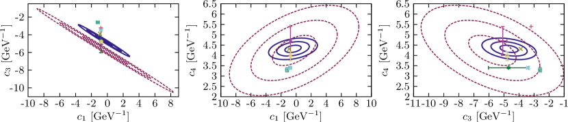
Figure 1: (Color online) Correlation ellipses of the chiral constants $c_{1}$, $c_{3}$ and $c_{4}$ determined from a fit to the self consistent database of Navarro Pérez et al. (2013b) with a DS-$\chi$TPE potential including data with $T_{\rm LAB}\leq 350$ Navarro Pérez et al. (2014a) (blue solid lines) and $T_{\rm LAB}\leq 125$ (red dashed lines). The concentric ellipses give, from the smallest to the largest one, the $68\%$, $95\%$ and $99\%$ confidence regions respectively. The points and crosses correspond to the determinations listed in Table VI of Navarro Pérez et al. (2014a)

The choice above is based on the high quality of our previous fit up to $T_{\rm LAB}=350{\rm MeV}$ which fulfills all needed statistical tests (see below). Our aim is that by reducing the energy range to $T_{\rm LAB}=125{\rm MeV}$ correlations among the parameters will appear implying a reduction of the number of independent parameters. Although the error of the data below $T_{\rm LAB}=125{\rm MeV}$ is the same, their induced propagation is amplified as a result of a fitting a smaller number of data. Even the observables computed below $125{\rm MeV}$ exhibit a larger error.

II.2 Fitting short distance parameters

Below $T_{\rm LAB}\leq 125$MeV the self-consistent data base obtained in Navarro Pérez et al. (2013b) contains $N_{pp}=925$ pp data and $N_{np}=1743$ np data including normalizations. This upper limit on the laboratory frame energy allows to reduce the number of parameters from $30$ in Navarro Pérez et al. (2014a) to $20$, appart from the $3$ chiral constants. Of course, with less data constraining the interaction the statistical uncertainties in the potential parameters are larger. The resulting delta-shell fitting parameters yield a total value of $\chi^{2}/\nu=1.02$ and are shown in Table 1. Note that to $1\sigma$ confidence level, one expects $\chi^{2}/\nu=1\pm\sqrt{2/\nu}$, which in this particular case means $0.097\leq\chi^{2}/\nu\leq 1.03$.

Table 1: Delta-shell parameters fitted to reproduce 2668 pp and np scattering data with $T_{\rm LAB}\leq 125$MeV. Statistical error bars are propagated from experimental uncertainties. The complete potential has a $\chi$TPE tail for $r>1.8$fm and all relevant electromagnetic interactions.

Wave	$\lambda_{1}$	$\lambda_{2}$	$\lambda_{3}$
	($r_{1}=0.6$fm)	($r_{1}=1.2$fm)	($r_{1}=1.8$fm)
${}^{1}S_{0}{\rm np}$	$0.88(79)$	$-0.75(19)$	$-0.053(46)$
${}^{1}S_{0}{\rm pp}$	$1.9(2)$	$-0.89(3)$	$-0.028(9)$
${}^{3}P_{0}$	$-$	$0.40(13)$	$-0.061(26)$
${}^{1}P_{1}$	$-$	$1.06(9)$	$-$
${}^{3}P_{1}$	$-$	$1.5(1)$	$0.016(13)$
${}^{3}S_{1}$	$1.6(6)$	$-$	$-$
$\varepsilon_{1}$	$-$	$-2.78(8)$	$-0.19(4)$
${}^{3}D_{1}$	$-$	$3.0(5)$	$-$
${}^{1}D_{2}$	$-$	$-0.58(7)$	$-$
${}^{3}D_{2}$	$-$	$-$	$-0.28(1)$
${}^{3}P_{2}$	$-$	$-0.44(1)$	$-$
$\varepsilon_{2}$	$-$	$-$	$0.097(11)$
${}^{3}F_{2}$	$-$	$-$	$-$
${}^{1}F_{3}$	$-$	$-$	$-$
${}^{3}D_{3}$	$-$	$1.1(1)$	$-$

This fit provides a new determination of the chiral constants $c_{1}=-0.27\pm 2.87$, $c_{3}=-5.77\pm 1.58$ and $c_{4}=4.24\pm 0.73$ GeV^-1 which is mostly compatible to the one from Navarro Pérez et al. (2014a). In Figure 1 we compare the ellipses of the present fit with those of our previous fit to 350 MeV Navarro Pérez et al. (2014a). Although each individual constant, with its corresponding $1\sigma$ confidence interval, is statistically compatible with the determination with data up to $T_{\rm LAB}=350$ MeV, the correlation ellipses of both fits for the $c_{1},c_{3}$ pair do not overlap.

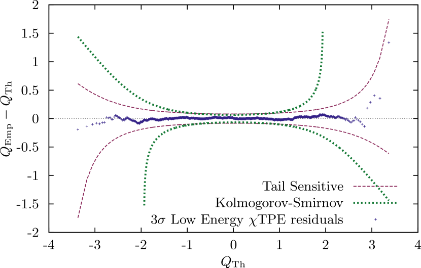
Figure 2: (Color online) Rotated quantile-quantile plot for the residuals of the low energy DS-$\chi$TPE potential for $E_{\rm LAB}\leq 125{\rm MeV}$ (blue crosses). The Kolmogorov-Smirnov (dotted green line) and Tail sensitive (dashed red line) confidence bands with an $\alpha=0.05$ significance level are also included.

III Scattering properties

III.1 Normality test

Once the potential parameters are fitted to the self-consistent data base we check the normality of the residuals

$$R_{i}=\frac{O_{i}^{\rm exp}-O_{i}^{\rm theo}}{\Delta O_{i}^{\rm exp}}.$$ (4)

To this end we apply the recently introduced Tail-Sensitive (TS) test Aldor-Noiman et al. (2013) (see Refs. Navarro Pérez et al. (2014b, c) for details and practical implementations). The TS test compares the quantiles of an empirical distribution with the quantiles of a normal distribution. The finite size of the sample gives a confidence interval for each quantile which can be calculated analytically for a previously determined significance level. If an empirical quantile falls outside of its corresponding confidence interval the hypothesis of normality is rejected. In figure 2 we show a rotated quantile-quantile (QQ) plot comparing the theoretical quantiles of the standard normal distribution $N(0,1)$ with the residuals quantiles; the confidence intervals for the TS and the more familiar Kolmogorov-Smirnov (KS) tests are also shown with a significance level $\alpha=0.05$. As can be seen, the empirical residuals resulting for the low energy fit always fall within the $95\%$ confidence bands of both the TS and KS normality tests.

Aside from obtaining a graphical representation, testing for normality is a straightforward procedure which simply requires to calculate a quantity known as a test statistic $T$ and compare it with a previously tabulated (or parameterized) critical value $T_{c}$ as a function of the sample size $N$. Depending on the definition of $T$ on each normality test, a larger (or conversely, smaller) $T$ indicates larger deviations from the normal distribution and $T>T_{c}$ (or $T<T_{c}$) gives significant evidence to reject the hypothesis of normality; in the particular case of the TS test large deviations from the normal distribution result in small values for $T$. For the TS test a recipe for calculating $T$, a table of $T_{c}$ for $N\leq 50$ and a parameterization for $50<N<9000$ can be found in Navarro Pérez et al. (2014c). The residuals of the low energy fit to the self consistent database give $T=0.0068$ and the critical value for a sample size $N=2668$ and a significance level $\alpha=0.05$ is $T_{c}=0.0008$ and therefore there is not significant evidence to reject the normality of the residuals.

III.2 Error propagation

Once the normality test is passed, we may proceed to propagate the errors inherited by the theory through the $\chi^{2}$-fit. We do so below for the phase shifts, the full scattering amplitude and the low energy threshold parameters. Several schemes are possible Navarro Perez et al. (2014): i) the standard covariance matrix of building derivatives in quadrature with correlations, ii) the Monte Carlo method based on a multivariate gaussian distribution based on the $\chi^{2}$ function, and iii) the more elaborated bootstrap method Navarro Perez et al. (2014). Results are fairly similar in all three cases and we use for definiteness the method ii). It consists of generating a sufficiently large sample drawn from a multivariate normal probability distribution

$$P(p_{1},p_{2},\ldots,p_{P})=\frac{1}{\sqrt{(2\pi)^{P}\det{\cal E}}}e^{-\frac{1}{2}({\bf p}-{\bf p}_{0})^{T}{\cal E}^{-1}({\bf p}-{\bf p}_{0})},$$ (5)

where ${\cal E}_{ij}=(\partial^{2}\chi/\partial p_{i}\partial p_{j})^{-1}$ is the error matrix and ${\bf p}_{0}$ are the fitting short distance $\lambda$’s and chiral $c$’s minimizing the $\chi^{2}$. We generate $M=1000$ samples ${\bf p}_{\alpha}\in P$ with $\alpha=1,\dots,M$, and compute $V_{NN}({\bf\lambda_{\alpha}})$ from which the corresponding observables are determined.

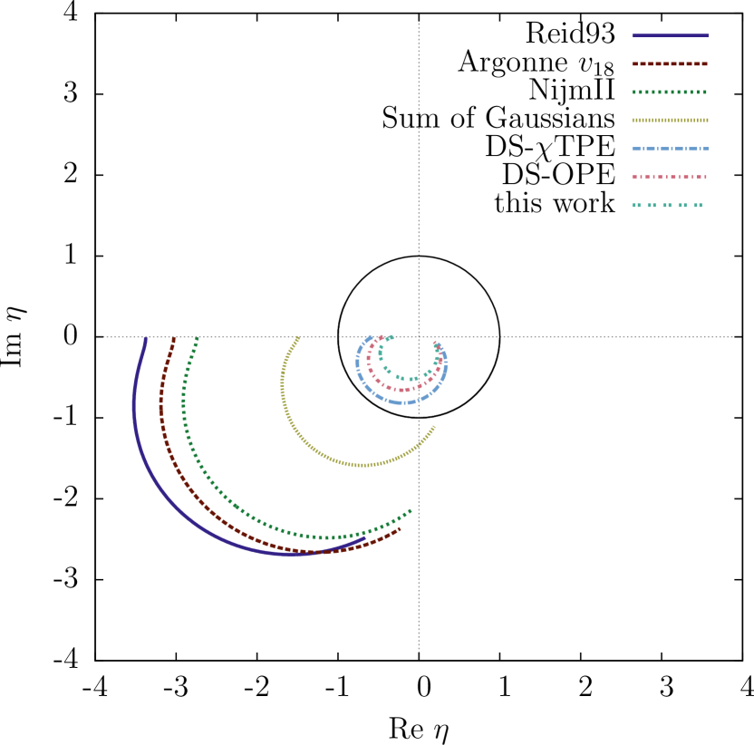
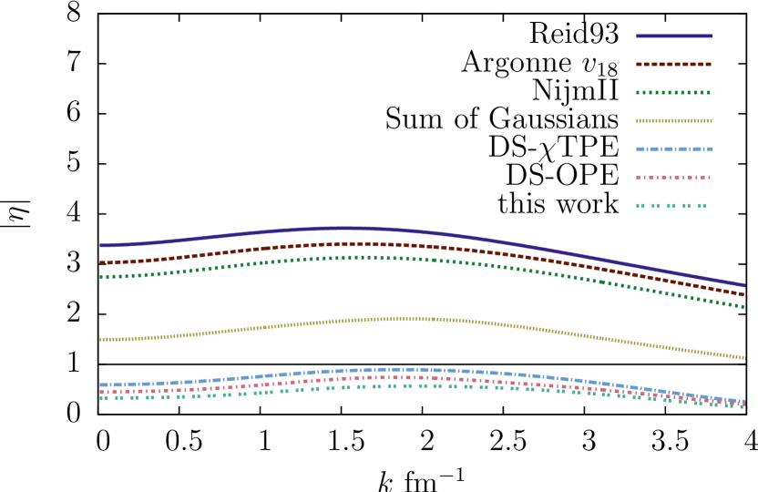
Figure 3: (Color online) Trajectories (upper pannel) and modulus (lower pannel) of the largest repulsive Weinberg eigenvalue in the ${}^{1}S_{0}$ channel as a funtion of CM momentum $k$ for high quality potentials. The potentials shown, ordered from largest to smalles modulus, are Reid93 Stoks et al. (1994), NijmII Stoks et al. (1994), AV18 Wiringa et al. (1995), Gauss-OPE Navarro Pérez et al. (2014b) DS-OPE Navarro Pérez et al. (2013a, b), DS-$\chi$TPE Navarro Pérez et al. (2014a, d), and the present work. We show the $|\eta|=1$ circle and line in a black solid line for reference

III.3 Softness of the potential

As we have mentioned in the introduction, restricting the fits to lower maximal energies becomes less sensitive to short distance details and hence one would expect satisfactory fits with softer cores to be eligible. As can be seen from a comparison of Table 1 with the corresponding one in the fit to $350$MeV Navarro Pérez et al. (2014a), the innermost strength coefficient has larger uncertainties than the previous higher energy fit. Thus, the softest edge of the confidence level could be used and still describe the data. A more quantitative measure of the softness of the potential is provided by the Weinberg eigenvalue analysis Weinberg (1963). Within the $V_{\rm lowk}$ approach Bogner et al. (2003); Anderson et al. (2008) this type of study has shown that there is an effective softening of the strong interaction by integrating out high CM momenta above $\Lambda\sim 2{\rm fm}^{-1}$ Bogner et al. (2006). The analysis there was mainly conducted in momentum space. So, we recapitulate the most relevant aspects in configuration space for completeness. The main idea is to solve the Schrödinger equation with a rescaled potential, $V\to V/\eta$ by a complex parameter $\eta$. In the uncoupled case the reduced wave equation reads

$$-w_{l,\nu}^{\prime\prime}(r)+\left[\frac{l(l+1)}{r^{2}}w_{l,\nu}+\frac{U_{l}(r)}{\eta_{l,\nu}(k)}\right]w_{l,\nu}(r)=k^{2}w_{l,\nu}(r)$$ (6)

with $U_{l}(r)=MV_{l}(r)$ the reduced potential. The solution is subject to the boundary conditions

$$w_{l,\nu}(r) \sim e^{ikr}\,,\qquad r\to\infty$$

$$w_{l,\nu}(r) \sim r^{l+1}\,,\qquad r\to 0$$ (7)

corresponding to a regular solution at the origin and outgoing spherical wave at infinity. On the upper lip of the positive energy scattering cut, $k\equiv\sqrt{k^{2}+i0^{+}}$ and the outgoing wave becomes the normalizable Weinberg eigenfunction $w_{l,\nu}(r)$ corresponding to the Weinberg eigenvalue $\eta_{l,\nu}(k)$. They are non-degenerate and are usually ordered according to the sequence $|\eta_{l,1}(k)|>|\eta_{l,2}(k)|>\dots$. In general $\eta_{l,\nu}(k)$ is complex and every single eigenvalue describes a trajectory in the complex plane as a function of the real momentum $k$. Clearly, for purely imaginary momentum $k=i\gamma$ with $\gamma>0$ one has an exponential fall-off $\sim e^{-\gamma r}$ typical of a bound state, such as, e.g., the deuteron whose energy is given by $E_{d}=-\gamma_{d}^{2}/M$. Thus, for the deuteron we have $\eta(i\gamma_{d})=1$. The important result is that the Born series for a given angular momentum $l$ and CM momentum $k$ converges if and only all eigenvalues are inside the unit circle in the complex plane, i.e., in particular $|\eta_{l,1}(k)|\equiv\max_{\nu}|\eta_{l,\nu}(k)|<1$. Finally, the size of $|\eta_{l,1}(k)|$ provides quantitative information on the convergence rate in perturbation theory of the scattering amplitude and hence of the Born series Weinberg (1963).

In Fig. 3 we show the trajectories and modulus as a function of $k$ for the largest Weinberg eigenvalue in the ${}^{1}S_{0}$ channel and for the high quality potentials NijmII Stoks et al. (1994), Reid93 Stoks et al. (1994), AV18 Wiringa et al. (1995) (shown for illustration) as well as our own high quality analyses using DS-OPE Navarro Pérez et al. (2013a, b), DS-$\chi$TPE Navarro Pérez et al. (2014a, d), the Gauss-OPE Navarro Pérez et al. (2014b) and the present work’s potentials. As we see, all the delta-shell potentials including OPE and TPE and the one of the present work generate Weinberg eigenvalues which are always inside the unit circle. The figure also convincingly shows that the coarse graining of the NN interaction via delta-shells actually yields a more perturbative potential when the maximum fitting energy range is lowered.

III.4 Phase-shifts

In Figure 4 we show the low angular momentum partial wave phase-shifts up to $T_{\rm LAB}=350$MeV for the low energy DS-$\chi$TPE and the DS-$\chi$TPE potential of Navarro Pérez et al. (2014a). The low energy version of the potential shows larger statistical uncertainties at higher energies since there are no data constraining the interaction above $125$ MeV. However, bellow this energy value statistical error bands are also larger for the low energy version of the potential. This indicates that the high energy data also play a significant role in determining the uncertainties at lower energies.

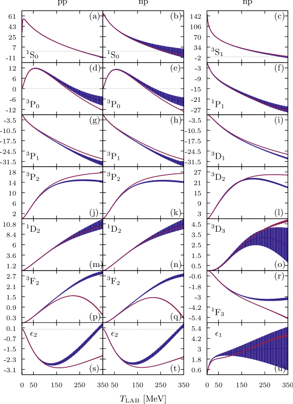
Figure 4: (Color online) Phase-shifts for the low energy DS-$\chi$TPE potential fitted to experimental data with $T_{\rm LAB}\leq 125$MeV with statistical error bans (blue bands). The corresponding phase-shifts and error bands for the full DS-$\chi$TPE reproducing data with $T_{\rm LAB}\leq 350$ MeV Navarro Pérez et al. (2014a) are also included for comparison (red bands)

III.5 Wolfenstein parameters

The full NN scattering amplitude reads

$$M = a+m(\mathbf{\sigma}_{1}\cdot\mathbf{n})(\mathbf{\sigma}_{2}\cdot\mathbf{n})+(g-h)(\mathbf{\sigma}_{1}\cdot\mathbf{m})(\mathbf{\sigma}_{2}\cdot\mathbf{m})$$ (8)

$$+ (g+h)(\mathbf{\sigma}_{1}\cdot\mathbf{l})(\mathbf{\sigma}_{2}\cdot\mathbf{l})+c(\mathbf{\sigma}_{1}+\mathbf{\sigma}_{2})\cdot\mathbf{n}$$

where the Wolfenstein parameters $a,m,g,h,c$ depend on energy and scattering angle, $\mathbf{\sigma}_{1}$ and $\mathbf{\sigma}_{2}$ are the single-nucleon Pauli matrices, $\mathbf{l}$, $\mathbf{m}$, $\mathbf{n}$ are three unitary orthogonal vectors along the directions of $\mathbf{k}_{f}+\mathbf{k}_{i}$, $\mathbf{k}_{f}-\mathbf{k}_{i}$ and $\mathbf{k}_{i}\wedge\mathbf{k}_{f}$, respectively, and ($\mathbf{k}_{f}$, $\mathbf{k}_{i}$) are the final and initial relative nucleon momenta. The relation with the phase shifts can be looked up in Refs. Glöckle (1983); Navarro Pérez et al. (2013b).

Figures 5, 6 and 7 compare the Wolfenstein parameters of the low energy DS-$\chi$TPE potential with the full DS-$\chi$TPE ones at $50$, $100$ and $200$ MeV respectively. At lower energies both interactions show a fair level of agreement and again the low energy version of the potential shows larger uncertainties. The discrepancies between both potentials, indicated by non-overlapping error bands, can be understood as the systematic uncertainties of both interactions. While at $200$MeV the discrepancies are much larger and hence beyond the range of validity of this new interaction, the dominance of systematic over statistical errors has been a recurrent feature. Actually, this worrysome pattern was pointed out in our early studies Navarro Pérez et al. (2012b, c) based on the Nijmegen-1993 analysis and it reappears almost ubiquitously in any of our own upgraded fits.

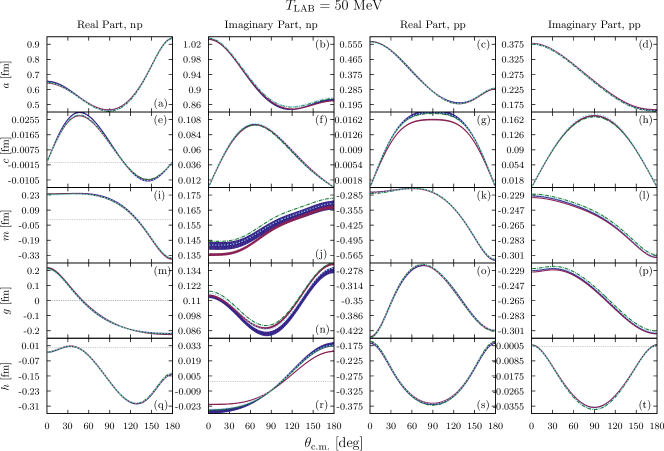
Figure 5: (Color online) $np$ (left) and $pp$ (right) Wolfenstein parameters (in fm) as a function of the c.m. angle (in degrees) and for $T_{\rm LAB}=50$MeV. We compare the low energy DS-$\chi$TPE potential (blue band) with full DS-$\chi$TPE potential Navarro Pérez et al. (2014a) (red band) the Nijmegen PWA Stoks et al. (1993a) (dotted, light blue line) and the AV18 potential Wiringa et al. (1995) (dashed-dotted, green line).

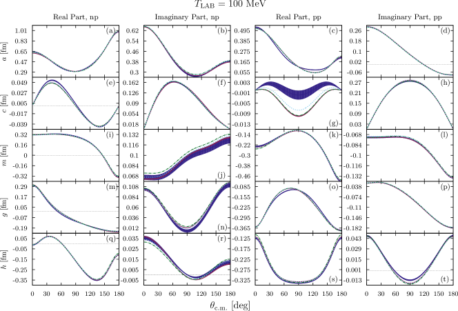
Figure 6: (Color online) Same as Fig. 5 but for $T_{\rm LAB}=100$MeV

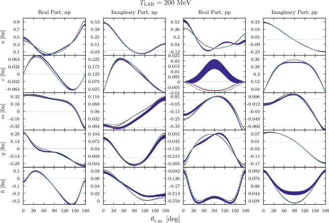
Figure 7: (Color online) Same as Fig. 5 but for $T_{\rm LAB}=200$MeV

III.6 Low energy threshold parameters

In the absence of tensor force the phase-shifts with angular momentum $l$ behave for low CM momentum, $k\to 0$, according to the effective range expansion

$$k^{2l+1}\cot\delta_{l}(k)=-\frac{1}{\alpha_{l}}+\frac{1}{2}r_{l}k^{2}+v_{2,l}k^{4}+\dots\,,$$ (9)

When the tensor force is considered we can apply a coupled channel generalization of the effective range expansion Pavon Valderrama and Ruiz Arriola (2005). Introducing the $\mathbf{\hat{M}}$ matrix defined as

$$\mathbf{DSD}^{-1}=\left(\mathbf{\hat{M}}+ik\mathbf{D}^{2}\right)\left(\mathbf{\hat{M}}-ik\mathbf{D}^{2}\right)^{-1},$$ (10)

where $\mathbf{S}$ is the usual unitary S-matrix and $\mathbf{D}={\rm diag}(k^{l_{1}},\ldots,k^{l_{N}})$. In the limit $k\to 0$, the $\mathbf{\hat{M}}$-matrix becomes

$$\mathbf{\hat{M}}=-\mathbf{a}^{-1}+\frac{1}{2}\mathbf{r}k^{2}+\mathbf{v_{2}}k^{4}+\mathbf{v_{3}}k^{6}+\mathbf{v_{4}}k^{8}+\dots,$$ (11)

where $\mathbf{a}$, $\mathbf{r}$ and $\mathbf{v_{i}}$ are the coupled channel generalizations of $\alpha_{0}$, $r_{0}$ and $v_{i}$ respectively. We have recently evaluated them and confronted statistical and systematic errors based on this expansion Perez et al. (2014b).

Table 2 shows the low energy threshold parameters of all partial waves with $j\leq 5$ for the low energy DS-$\chi$TPE potential. The statistical uncertainties are propagated by drawing $1000$ random sets of potential parameters following a multivariate normal distribution according to the covariance matrix, calculating the low energy threshold parameters for each set of parameters and taking the mean and standard deviation.

Table 2: Low energy threshold parameters for all partial waves with $j\leq 5$ for the DS-$\chi$TPE potential. The central value and statistical error bars correspond to the mean and standard deviation of a population of $1000$ parameters calculated with a Monte Carlo family of potential parameters drawn according the the covariance matrix of the potential parameters. For each partial wave we show the scattering length $\alpha$, the effective range $r_{0}$ and the curvature parameters $v_{2}$, $v_{3}$ and $v_{4}$. For the coupled channels we use the nuclear bar parameterization of the $S$ matrix. The units are in powers of femtometers determined by the orbital angular momentum quantum numbers $l$ and $l^{\prime}$ of each partial wave

Wave	$\alpha({\rm fm}^{l+l^{\prime}+1})$	$r_{0}({\rm fm}^{l+l^{\prime}+1})$	$v_{2}({\rm fm}^{l+l^{\prime}+3})$	$v_{3}({\rm fm}^{l+l^{\prime}+5})$	$v_{4}({\rm fm}^{l+l^{\prime}+7})$
${}^{1}S_{0}$	$-23.739975$	$2.683075$	$-0.482309$	$3.876303$	$-19.536951$
	$\pm 0.019856$	$\pm 0.010688$	$\pm 0.010963$	$\pm 0.043940$	$\pm 0.122646$
${}^{3}P_{0}$	$-2.497645$	$3.809329$	$1.006610$	$3.861832$	$-7.889673$
	$\pm 0.007007$	$\pm 0.017893$	$\pm 0.013141$	$\pm 0.044996$	$\pm 0.083544$
${}^{1}P_{1}$	$2.780145$	$-6.461193$	$-1.707267$	$0.293702$	$7.970193$
	$\pm 0.008084$	$\pm 0.029229$	$\pm 0.050329$	$\pm 0.094128$	$\pm 0.083765$
${}^{3}P_{1}$	$1.514034$	$-8.667588$	$0.014268$	$-0.504544$	$-0.583288$
	$\pm 0.002833$	$\pm 0.022467$	$\pm 0.026836$	$\pm 0.070704$	$\pm 0.204727$
${}^{3}S_{1}$	$5.424721$	$1.833010$	$-0.120574$	$1.433963$	$-7.563664$
	$\pm 0.001887$	$\pm 0.003057$	$\pm 0.002884$	$\pm 0.008492$	$\pm 0.036475$
$\epsilon_{1}$	$1.686135$	$0.426075$	$-0.243444$	$1.436825$	$-7.260537$
	$\pm 0.013563$	$\pm 0.006913$	$\pm 0.010099$	$\pm 0.016457$	$\pm 0.019671$
${}^{3}D_{1}$	$6.563492$	$-3.493365$	$-3.645026$	$1.135239$	$-2.638623$
	$\pm 0.026034$	$\pm 0.013119$	$\pm 0.021307$	$\pm 0.017822$	$\pm 0.020137$
${}^{1}D_{2}$	$-1.385117$	$14.895810$	$16.422846$	$-12.890261$	$37.903278$
	$\pm 0.002580$	$\pm 0.045677$	$\pm 0.118270$	$\pm 0.193378$	$\pm 0.601827$
${}^{3}D_{2}$	$-7.408744$	$2.851102$	$2.360846$	$-1.083437$	$1.753274$
	$\pm 0.005410$	$\pm 0.003869$	$\pm 0.012195$	$\pm 0.026133$	$\pm 0.026984$
${}^{3}P_{2}$	$-0.297390$	$-8.478863$	$-7.433750$	$-7.477923$	$-14.511322$
	$\pm 0.003170$	$\pm 0.046753$	$\pm 0.145525$	$\pm 0.416712$	$\pm 0.788810$
$\epsilon_{2}$	$1.600387$	$-15.966142$	$-25.930128$	$-25.222196$	$-70.658514$
	$\pm 0.001190$	$\pm 0.043977$	$\pm 0.168760$	$\pm 0.682425$	$\pm 1.762290$
${}^{3}F_{2}$	$-0.974812$	$-5.957998$	$-24.133336$	$-83.161809$	$-124.079013$
	$\pm 0.001774$	$\pm 0.058571$	$\pm 0.209295$	$\pm 0.899196$	$\pm 3.081428$
${}^{1}F_{3}$	$8.377225$	$-3.925084$	$-9.873666$	$-15.298794$	$-2.050820$
	$\pm 0.002234$	$\pm 0.001881$	$\pm 0.010626$	$\pm 0.056008$	$\pm 0.129186$
${}^{3}F_{3}$	$2.680008$	$-10.037798$	$-20.952701$	$-20.389419$	$-30.275280$
	$\pm 0.001765$	$\pm 0.011854$	$\pm 0.056074$	$\pm 0.257995$	$\pm 0.643766$
${}^{3}D_{3}$	$-0.140354$	$1.371004$	$2.071825$	$1.913193$	$-0.549459$
	$\pm 0.002730$	$\pm 0.000773$	$\pm 0.003553$	$\pm 0.013570$	$\pm 0.019826$
$\epsilon_{3}$	$-9.682379$	$3.260401$	$7.672521$	$9.579540$	$-1.135140$
	$\pm 0.000465$	$\pm 0.000832$	$\pm 0.004167$	$\pm 0.019404$	$\pm 0.047122$
${}^{3}G_{3}$	$4.874337$	$-0.030192$	$0.001640$	$-0.003425$	$-2.718540$
	$\pm 0.000639$	$\pm 0.001672$	$\pm 0.009409$	$\pm 0.051735$	$\pm 0.151814$
${}^{1}G_{4}$	$-3.212045$	$10.809086$	$34.473444$	$81.971319$	$104.049040$
	$\pm 0.000661$	$\pm 0.003870$	$\pm 0.024269$	$\pm 0.155640$	$\pm 0.521681$
${}^{3}G_{4}$	$-19.145092$	$2.058351$	$6.814736$	$16.772767$	$10.019825$
	$\pm 0.000743$	$\pm 0.000143$	$\pm 0.001002$	$\pm 0.007057$	$\pm 0.025122$
${}^{3}F_{4}$	$-0.016002$	$-3.053099$	$-4.815627$	$73.726022$	$664.426931$
	$\pm 0.001726$	$\pm 0.002105$	$\pm 0.012043$	$\pm 0.055466$	$\pm 0.126890$
$\epsilon_{4}$	$3.585807$	$-9.548329$	$-37.136343$	$-185.113250$	$-587.360666$
	$\pm 0.000044$	$\pm 0.002591$	$\pm 0.014979$	$\pm 0.061061$	$\pm 0.413503$
${}^{3}H_{4}$	$-1.240294$	$-0.204717$	$-1.772049$	$-17.439098$	$-123.030299$
	$\pm 0.000290$	$\pm 0.008206$	$\pm 0.059293$	$\pm 0.551235$	$\pm 3.669909$
${}^{1}H_{5}$	$28.573515$	$-1.726914$	$-7.906396$	$-32.787619$	$-59.367511$
	$\pm 0.000317$	$\pm 0.000034$	$\pm 0.000320$	$\pm 0.003254$	$\pm 0.019300$
${}^{3}H_{5}$	$6.079919$	$-6.440909$	$-25.238708$	$-82.597219$	$-168.850963$
	$\pm 0.000281$	$\pm 0.000514$	$\pm 0.003801$	$\pm 0.030382$	$\pm 0.140866$
${}^{3}G_{5}$	$-0.009639$	$0.480549$	$1.878389$	$6.098743$	$6.785788$
	$\pm 0.000646$	$\pm 0.000017$	$\pm 0.000142$	$\pm 0.001302$	$\pm 0.006672$
$\epsilon_{5}$	$-31.301936$	$1.556146$	$6.994315$	$28.175241$	$48.356412$
	$\pm 0.000033$	$\pm 0.000020$	$\pm 0.000180$	$\pm 0.001704$	$\pm 0.009264$
${}^{3}I_{5}$	$10.677985$	$0.010777$	$0.144456$	$1.427543$	$6.457572$
	$\pm 0.000110$	$\pm 0.000058$	$\pm 0.000542$	$\pm 0.005504$	$\pm 0.032654$

IV Effective interactions at low momentum

We now turn to analyze the corresponding potential in momentum space, particularly within a low momentum expansion. As we have shown elsewhere Navarro Pérez et al. (2013d), the coefficients of the expansion can be mapped into radial moments of volume integrals of the potential, which exhibit some degree of universality. We will separate the contributions stemming from the inner region $r<r_{c}$ containing just delta-shell interactions and the outer region $r>r_{c}$ containing the pion exchange potential tail. For ease of comparison, we will consider the results in a Cartesian as well as in the spherical basis.

IV.1 Moshinsky-Skyrme parameters

At the two body level the effective interaction of Moshinsky Moshinsky (1958) and Skyrme Skyrme (1959) can be written as a pseudo-potential in the form

$$V_{\Lambda}({\bf p}^{\prime},{\bf p})=\int d^{3}xe^{-i{\bf x}\cdot({\bf p^{\prime}}-{\bf p})}\hat{V}({\bf x})$$

$$=t_{0}(1+x_{0}P_{\sigma})+\frac{t_{1}}{2}(1+x_{1}P_{\sigma})({\bf p}^{\prime 2}+{\bf p}^{2})$$

$$+t_{2}(1+x_{2}P_{\sigma}){\bf p}^{\prime}\cdot{\bf p}+2iW_{0}{\bf S}\cdot({\bf p}^{\prime}\wedge{\bf p})$$ (12)

$$+\frac{t_{T}}{2}\left[\sigma_{1}\cdot{\bf p}\,\sigma_{2}\cdot{\bf p}+\sigma_{1}\cdot{\bf p^{\prime}}\,\sigma_{2}\cdot{\bf p^{\prime}}-\frac{1}{3}\sigma_{1}\,\cdot\sigma_{2}({\bf p^{\prime}}^{2}+{\bf p}^{2})\right]$$

$$+\frac{t_{U}}{2}\left[\sigma_{1}\cdot{\bf p}\,\sigma_{2}\cdot{\bf p}^{\prime}+\sigma_{1}\cdot{\bf p^{\prime}}\,\sigma_{2}\cdot{\bf p}-\frac{2}{3}\sigma_{1}\,\cdot\sigma_{2}{\bf p^{\prime}}\cdot{\bf p}\right]+{\cal O}(p^{4})$$

where $P_{\sigma}=(1+\sigma_{1}\cdot\sigma_{2})/2$ is the spin exchange operator with $P_{\sigma}=-1$ for spin singlet ($S=0$), and $P_{\sigma}=1$ for spin triplet ($S=1$) states.

The effective interaction representation in terms of Moshinsky-Skyrme parameters are presented in tables 3. Since both parameterizations consist of potential integrals, see Ref. Navarro Pérez et al. (2013d), we show the contribution to the full parameter by the phenomenological short range part $r\leq r_{c}$ and the pion exchange tail $r>r_{c}$ with the corresponding uncertainties. Since the potential is determined by low energy data only, one would expect the short range contribution to counter-terms of the most peripheral partial waves to be compatible with zero. However, we see that although the errors are larger than those quoted in Navarro Pérez et al. (2014c) for a DS-$\chi$TPE potential fitted to data up to $350$MeV, the short range counter-terms are never compatible with zero. It is also worth noting that the full integrals both for Moshinsky-Skyrme parameters and counter-terms show a large degree of universality when compared to the same parameters for the DS-OPE and DS-$\chi$TPE potentials shown in Navarro Pérez et al. (2014c).

IV.2 Counter-Terms

The potential in momentum space can be written in the partial wave basis as

$$v^{JS}_{l^{\prime},l}(p^{\prime},p)=(4\pi)^{2}\int_{0}^{\infty}\,dr\,r^{2}\,j_{l^{\prime}}(p^{\prime}r)j_{l}(pr)V_{l^{\prime}l}^{JS}(r)\,$$ (13)

Using the Bessel function expansion for small argument $j_{l}(x)=x^{l}/(2l+1)!![1-x^{2}/2(2l+3)+\dots]$ we get a low momentum expansion of the potential matrix elements. We keep up to total order ${\cal O}(p^{4},p^{\prime 4},p^{2}p^{\prime 2})$ corresponding to $S$-, $P$- and $D$-waves as well as S-D and P-F mixing parameters,

$$v_{00}^{JS}(p^{\prime},p) = \widetilde{C}_{00}^{JS}+C_{00}^{JS}(p^{2}+p^{\prime 2})+D^{1}_{00}{}^{JS}(p^{4}+p^{\prime 4})$$

$$+ D^{2}_{00}{}^{JS}p^{2}p^{\prime 2}+\cdots$$

$$v_{11}^{JS}(p^{\prime},p) = pp^{\prime}C_{11}^{JS}+pp^{\prime}(p^{2}+p^{\prime 2})D_{11}^{JS}+\cdots$$

$$v_{22}^{JS}(p^{\prime},p) = p^{2}p^{\prime}{}^{2}D_{22}^{JS}+\cdots$$

$$v_{20}^{JS}(p^{\prime},p) = p^{\prime}{}^{2}C_{20}^{JS}+p^{\prime}{}^{2}p^{2}D^{1}_{20}{}^{JS}+p^{\prime}{}^{4}D^{2}_{20}{}^{JS}+\dots$$

$$v_{31}^{JS}(p^{\prime},p) = p^{\prime}{}^{3}pD_{31}^{JS}+\cdots$$ (14)

We use the spectroscopic notation and normalization of Ref. Epelbaum et al. (2005). The numerical results are shown in Table 4. We see, again, a magnification of errors in the short range contribution due to the lowering of the energy from $350{\rm MeV}$ to $125{\rm MeV}$ and a confirmation of the universality between OPE and $\chi$TPE unveiled in Ref. Navarro Pérez et al. (2014c). Actually we found a correlation pattern which qualifies these counter-terms as good fitting parameters, i.e. small statistical dependence and scheme independence.

Table 3: Moshinsky-Skyrme parameters. We separate the contribution from the delta-shells short range parameters (corresponding to $r<r_{c}=1.8$fm) and the $\chi$TPE potential tail (corresponding to $r>r_{c}$) . Units are: $t_{0}$ in ${\rm MeV}{\rm fm}^{3}$, $t_{1},t_{2},W_{0},t_{U},t_{T}$ in ${\rm MeV}{\rm fm}^{5}$, and $x_{0},x_{1},x_{2}$ are dimensionless.

	$r<r_{c}$	$r>r_{c}$	Full
$t_{0}$	$-87.8(729)$	$-382.3(91)$	$-470.1(767)$
$x_{0}$	$-4.5(40)$	$-0.088(2)$	$-0.92(23)$
$t_{1}$	$77.2(98)$	$821.0(57)$	$898.1(117)$
$x_{1}$	$-1.2(1)$	$-0.00832(6)$	$-0.11(1)$
$t_{2}$	$243.1(195)$	$2212.5(159)$	$2455.6(113)$
$x_{2}$	$-0.58(4)$	$-0.911(2)$	$-0.877(3)$
$W_{0}$	$105.8(30)$	$4.7$	$110.5(30)$
$t_{U}$	$148.1(49)$	$1132.8(30)$	$1281.0(56)$
$t_{T}$	$-569.4(301)$	$-3836.0(90)$	$-4405.4(279)$

Table 4: Potential integrals in different partial waves. We separate the contribution from the delta-shells short range parameters (corresponding to $r<r_{c}=1.8$fm) and the $\chi$TPE potential tail (corresponding to $r>r_{c}$) . Units are: $\widetilde{C}$’s are in $10^{4}{\rm GeV}^{-2}$, $C$’s are in $10^{4}{\rm GeV}^{-4}$ and $D$’s are in $10^{4}{\rm GeV}^{-6}$.

	$r<r_{c}$	$r>r_{c}$	Full
$\widetilde{C}_{{}^{1}S_{0}}$	$-0.079(14)$	$-0.068(1)$	$-0.15(1)$
$C_{{}^{1}S_{0}}$	$0.73(8)$	$3.48(2)$	$4.20(8)$
$D_{{}^{1}S_{0}}^{1}$	$-6.2(17)$	$-440.5(8)$	$-446.7(19)$
$D_{{}^{1}S_{0}}^{2}$	$-1.9(5)$	$-132.1(2)$	$-134.0(6)$
$\widetilde{C}_{{}^{3}S_{1}}$	$0.051(18)$	$-0.057(1)$	$-0.006(19)$
$C_{{}^{3}S_{1}}$	$-0.078(28)$	$3.42(2)$	$3.34(4)$
$D_{{}^{3}S_{1}}^{1}$	$0.12(4)$	$-503.7(8)$	$-503.6(8)$
$D_{{}^{1}S_{0}}^{2}$	$0.036(13)$	$-151.1(2)$	$-151.1(2)$
$C_{{}^{1}P_{1}}$	$0.54(5)$	$5.92(4)$	$6.45(3)$
$D_{{}^{1}P_{1}}$	$-2.0(2)$	$-588.8(9)$	$-590.8(8)$
$C_{{}^{3}P_{1}}$	$0.79(3)$	$2.934(8)$	$3.72(3)$
$D_{{}^{3}P_{1}}$	$-3.09(9)$	$-246.1(3)$	$-249.2(4)$
$C_{{}^{3}P_{0}}$	$0.046(12)$	$-4.98(2)$	$-4.94(1)$
$D_{{}^{3}P_{0}}$	$0.55(32)$	$343.7(6)$	$344.2(5)$
$C_{{}^{3}P_{2}}$	$-0.221(5)$	$-0.265(9)$	$-0.486(8)$
$D_{{}^{3}P_{2}}$	$0.82(2)$	$-9.6(4)$	$-8.8(4)$
$D_{{}^{1}D_{2}}$	$-0.44(5)$	$-70.5(1)$	$-70.9(1)$
$D_{{}^{3}D_{2}}$	$-2.4(1)$	$-363.0(2)$	$-365.4(2)$
$D_{{}^{3}D_{1}}$	$2.2(3)$	$202.3(2)$	$204.5(3)$
$D_{{}^{3}D_{3}}$	$0.80(11)$	$-0.13(14)$	$0.67(16)$
$C_{\epsilon_{1}}$	$-1.13(6)$	$-7.60(2)$	$-8.72(6)$
$D_{\epsilon_{1}}^{1}$	$9.1(9)$	$998.9(5)$	$1008.0(8)$
$D_{\epsilon_{1}}^{2}$	$3.9(4)$	$428.1(2)$	$432.0(3)$
$D_{\epsilon_{2}}$	$0.59(7)$	$82.59(5)$	$83.18(6)$

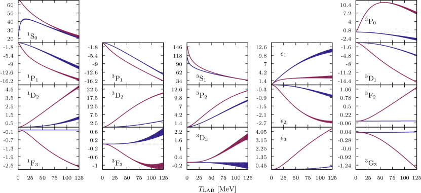
Figure 8: (Color online) Short distance phase-shifts with statistical error bands in degrees (blue bands) for the $\delta$-shell $\chi$TPE-potential fitted up to a maximum ${\rm E_{\rm LAB}}=125{\rm MeV}$ obtained by eliminating all contributions of the potential with $r\geq 1.8{\rm fm}$ and keeping just the Delta-shells potential (see main text). The complete phase-shifts (red bands) are drawn for comparison.

IV.3 Short distance phase-shifts

A complementary way to visualize the short distance structure of the theory is by looking at the corresponding phase-shifts, $\delta^{\rm Short}_{l}$, which are those corresponding just to the short distance part of the potential $V_{\rm DS}(r)$ in Eq. (1). Because $V_{\rm DS}(r)$ has a range of $r_{c}=1.8{\rm fm}$ the partial wave expansion will converge for $l_{\rm max}=pr_{c}$, and so we expect $\delta^{\rm Short}_{l_{\rm max}+1}\simeq 0$ within the theoretical uncertainties. In our case $l_{\rm max}=2$ which corresponds to D-waves, and so we expect F, G and higher waves to produce negligible phase-shifts from the short distance piece of the potential $V_{\rm DS}(r)$ in Eq. (1). This is illustrated in Fig. 8, where F and G phase-shifts are very small except for the marginal ${}^{3}F_{3}$ wave around $\simeq 100$ MeV.

We note that similar findings have been pointed out in the deconstruction analysis of Ref. Birse and McGovern (2004) based on the Nijmegen partial wave analysis. Our present study includes more and coupled channels and takes statistical errors into account.

IV.4 Cut-off dependence

Our delta-shell potential can be interpreted as a UV regulator, where $\Delta r\sim 1/\Lambda$ is the resolution scale and the short distance cut-off $r_{c}$ the scale below which the interaction is unknown . It is interesting to consider the short distance cut-off dependence. Actually we can try to replace the outermost delta-shells by the TPE potential, that is, making $r_{c}=1.2$fm and therefore a further reduction of parameters would take place. Moreover, restricting the fit to lower energies corresponds to have about a twice larger shortest de Broglie wavelength. Thus, one may naturally hope to be more blind to the nucleon finite size effects.

We want to analyze here four possible effects, namely the modifications due to i) taking fixed (and $\pi N$ motivated) chiral constants vs NN fitted, ii) the counterterm structure, iii) the change in the maximum fitted energy and iv) reduction of the short distance cut-off.

Table 5: Different delta-shell potentials with chiral two pion exchange tail fitted to the self-consistent Granada database of Navarro Pérez et al. (2013b). The first line corresponds to the potential presented in Navarro Pérez et al. (2014a) and the second line to the potential of this work. The chiral constants of the fourth line were taken from a Ref. Ekström et al. (2013, 2014) and used as fixed values during the $\chi^{2}$ minimization with respect of the delta-shell parameters. Highest counterterm column indicates the maximum angular momentum where at least one delta-shell strength coefficient is non-vanishing.

Max $T_{\rm LAB}$	$r_{c}$	$c_{1}$	$c_{3}$	$c_{4}$	Highest	$\chi^{2}/\nu$
MeV	fm	GeV-1	GeV-1	GeV-1	counterterm
350	1.8	$-0.4(11)$	$-4.7(6)$	$4.3(2)$	$F$	1.08
350	1.2	$-9.8(2)$	$0.3(1)$	$2.84(5)$	$F$	1.26
125	1.8	$-0.3(29)$	$-5.8(16)$	$4.2(7)$	$D$	1.03
125	1.2	$-0.92$	$-3.89$	$4.31$	$P$	1.70
125	1.2	$-14.9(6)$	$2.7(2)$	$3.51(9)$	$P$	1.05

The results are summarized in table 5 and we proceed to discuss them. For instance, when we return to our DS-$\chi$TPE fit up to $T_{\rm lab}=350$MeV, we find that this cut-off reduction from $r_{c}=1.8$fm to $r_{c}=1.2$fm produces after refitting parameters $\chi^{2}/N\sim 1.26$ with chiral constants $c_{1,3,4}=-9.77,0.31,2.84$Gev^-1. Notice the unnaturally large value for $c_{1}$ and how $c_{3}$ has positive value while most other determinations from $\pi$N and NN give a negative value. We view these features as a manifestation of the finite size effects of the nucleon which become visible at the energy range extending up to pion production threshold. A recent analysis of a Minimally non-local (and continuous, i.e. plotable) nucleon-nucleon potentials with chiral two-pion exchange including $\Delta$’s fully agrees with this finding Piarulli et al. (2014), namely a similar increase of the $\chi^{2}/\nu=1.3$, with a family of short distance potentials which operate around $1.1{\rm fm}$.

We now discuss the influence of the counterterm structure, namely which partial waves are parameterized with the delta-shells interpreted as an UV regulator. Thus, we may remove the $r\leq r_{c}$ contribution to a given counterterm by setting all delta-shell strength coefficients to zero in the corresponding partial wave . If we take now the fixed chiral constants of Ref. Ekström et al. (2013, 2014), and assume the same counterterms structure on each partial wave and fit to our database up to $T_{\rm LAB}=125$Mev with our delta-shell inner potential and $r_{c}=1.2$fm we get a statistically significantly larger $\chi^{2}/N=1.7$. With this same structure one can substantially reduce this value down to $\chi^{2}/N=1.05$ when the chiral contants are allowed to vary. Their values $c_{1,3,4}=-14.87,2,71,3.51$GeV^-1 are again unnaturally large for $c_{1}$ and with the wrong sign for $c_{3}$.

IV.5 Discussion

We see that a feature of our calculation is that a fit up to $T_{\rm LAB}=125{\rm MeV}$ fulfilling a good $\chi^{2}/\nu=1.02$ and passing the normality test requires in addition to the $\chi$TPE potential non-vanishing short distance contributions for S, P and D waves, $\delta^{\rm Short}_{l}$. As shown, a way of reducing short distance D-wave phase-shifts is by reducing the value of $l_{\rm max}=p_{\rm max}r_{c}$ to $\sim 1$. This can be achieved either by reducing $r_{c}$ below $1.8\,{\rm fm}$ or $p_{\rm max}$ or both. For instance, choosing $p_{\rm max}=m_{\pi}$ would correspond to $E_{\rm LAB}\leq 40{\rm MeV}$. Alternatively, one may choose $r_{c}=1{\rm fm}$ and keep $E_{\rm LAB}\leq 125{\rm MeV}$. According to our findings in subsection IV.4 and our discussion on the anatomy of the $NN$-potential Navarro Pérez et al. (2014d) taking $r_{c}\lesssim 1.8{\rm fm}$ the nucleon size and quark exchange effects start playing a role and the elementary particle assumption , upon which our NN-potential approach is based, becomes debatable.

V Comparison with other low energy chiral potentials

This work introduces a new phenomenological Nucleon-Nucleon chiral two-pion exchange potential fitted to pp and np scattering data up to a laboratory energy of $125$MeV similar in spirit to other recent low energy chiral interactions Ekström et al. (2013); Gezerlis et al. (2013); Ekström et al. (2014); Gezerlis et al. (2014) which have become popular in nuclear structure calculations. We comment now on both approaches and the major differences with ours from a statistical point of view.

V.1 Momentum space optimized chiral potential at NNLO

The momentum space self-denominated optimized chiral nucleon-nucleon interaction at next-to-next-to-leading order potential Ekström et al. (2013) provides a moderately acceptable $\chi^{2}/\nu=1.16$ value. It is based on the 1999 update of the Nijmegen Stoks et al. (1993a, 1994) database done with the event of the CD Bonn potential analysis Machleidt (2001) with some minor modifications. With $\nu=N-P=1945-24$ degrees of freedom, one should expect within $68\%$ confidence level a value $\chi^{2}/\nu=1\pm\sqrt{2\nu}=1\pm 0.03$, which is excluded by $5\sigma$ . In the standard statistical jargon this means that the there is probability $\sim 10^{-7}$ of erring when saying that the distribution does not obey a $\chi^{2}$ distribution. As we have stressed in our previous worksNavarro Pérez et al. (2014b, c), one may re-scale a too large $\chi^{2}$ by a Birge factor to a new $\bar{\chi}^{2}=(\chi^{2}/\chi^{2}_{\rm min})\nu$, which by definition fulfills $\bar{\chi}^{2}_{\rm min}/\nu=1$, provided the residuals of the fit are normally distributed. In this case, a re-scaling of experimental uncertainties, namely $\Delta O_{i}^{\rm exp}\to\sqrt{\chi^{2}_{\rm min}/\nu}\Delta O_{i}^{\rm exp}=\sqrt{1.16}\Delta O_{i}^{\rm exp}$, would correspond to a bearable $7\%$ uncertainty in the error (the error of the error). This is the kind of situation (too large $\chi^{2}/\nu$) where the check for normality would be most useful. 

In Ref. Ekström et al. (2014) the reported skewness and excess kurtosis of the histogram of residuals are $\Delta\mu_{3}^{\prime}=0.06$ and $\Delta\mu_{4}^{\prime}=0.37$, respectively. The latter value is a bit too high. Indeed, within a $68\%$ ($1\sigma$) confidence level we should have $\Delta\mu_{3}^{\prime}=\sqrt{17/\nu}$ and $\Delta\mu_{4}^{\prime}=4\sqrt{6/\nu}$, i.e. $\Delta\mu_{3}^{\prime}=0.09$ and $\Delta\mu_{4}^{\prime}=0.22$ respectively. The lack of normality is better unveiled in terms of their QQ-plot. They show a line resembling, $Q_{\rm Emp}\sim 1.35Q_{\rm Th}$  Ekström et al. (2014) instead of the expected $Q_{\rm Emp}\sim Q_{\rm Th}$ straight line. To better compare with our Fig. 2, that situation is recreated in a rotated QQ-plot in Fig. 9 where the confidence bands are adapted to the features of Ref. Ekström et al. (2014). 

Figure 9: (Color online) Rotated quantile-quantile plot for the residuals of the low energy optimized momentum space chiral potential of Ref. Ekström et al. (2014) (dark blue crosses). The scaled (yellow crosses) and standardized (light blue crosses) are also shown. The Kolmogorov-Smirnov (dotted green line) and Tail sensitive (dashed red line) confidence bands with an $\alpha=0.05$ significance level are also included.

Since in Refs. Ekström et al. (2013, 2014) a different database from our $3\sigma$ self-consistent one was adopted, one may think that re-doing the analysis might improve the normality properties of the fit. This is unlikely, because normality requires enough flexibility of the theory to encompass the fitted data up to statistical fluctuations which are tolerated only thanks to the finite number of data. Increasing the database should naturally decrease the fluctuations. In our case, we have $N=925_{pp}+1743_{np}=2688$ data including normalizations vs the $N=1945$ data used in Refs. Ekström et al. (2013, 2014). It is unlikely that the bias introduced in the analysis of Refs. Ekström et al. (2013, 2014) will be compensated by adding about 700 extra data. Thus, we attribute the lack of normality to a lack of flexibility in the proposed interaction. The question whether our self-consistent database is itself biased by our own analysis is a pertinent one, but this could only be answered by re-doing a data selection anew from scratch. Such an independent data selection analysis would be most welcome to sort out these issues.

V.2 Local chiral potential

The local chiral potentials Gezerlis et al. (2013, 2014) fit phase shifts or low energy parameters in the lowest partial waves taken as independent data and provide a sequence of LO,NLO and NNLO schemes. An important feature of this potential concerns the regulator which corresponds to a short distance potential of a range about $1-1.2{\rm fm}$. We have implemented this potential and checked that their phase-shifts are reproduced for all schemes. We can thus confront this potential to the np and pp database and compute the total $\chi^{2}$ as a function of the maximal LAB energy. The result is shown in Fig. 10 and as we see the smallest value we get is $\chi^{2}/N\gtrsim 1$ for $T_{\rm LAB}\sim 40{\rm MeV}$. Nonetheless, our experience in comparing phase-shift with PWA fits suggests that much better values could be achieved with relatively small parameter changes. This is possibly an effect due to the correlations among phase-shifts which in Ref. Gezerlis et al. (2013, 2014) are certainly ignored. Given their wide applicability in nuclear structure calculations, it would be interesting to perform a full PWA of these local chiral potentials and test their normality.

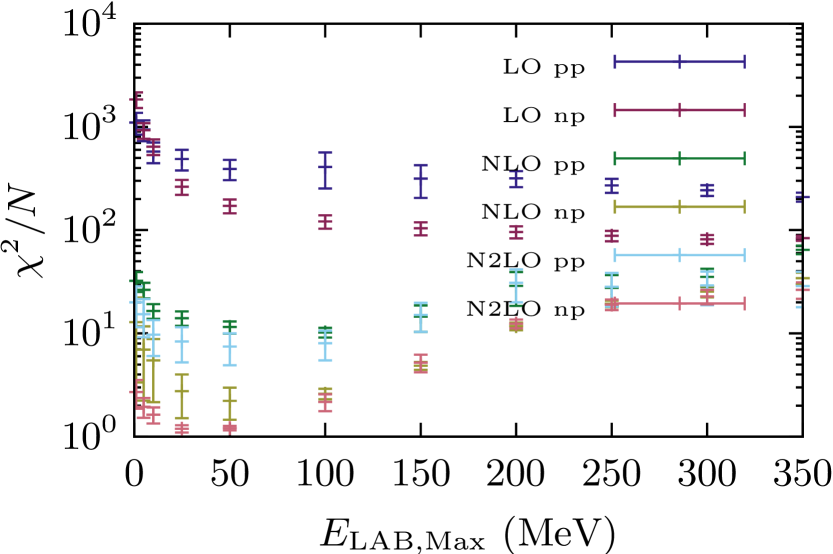
Figure 10: (Color online) Values of $\chi^{2}/N$ for the local chiral potentials of Ref. Gezerlis et al. (2014) as a function of the maximum LAB energy (in MeV). We distinguish the different contributions building their LO,NLO and NNLO for np and pp.

V.3 Discussion

While the features of both the momentum space and the coordinate space treatments discussed above are different regarding their implementation details and statistical behavior, they share with our present analysis the same chiral potential Kaiser et al. (1997) at long distances $r\gtrsim 2{\rm fm}$. The main difference relies in the way the short distance pieces of the interaction are represented. As we have mentioned Chiral perturbation theory ($\chi$pt) provides a power counting scheme to systematically include pion exchange interactions in the complete NN potential Weinberg (1990); Ordonez and van Kolck (1992). The several phenomenological chiral potentials which have appeared in the literature include the $\chi$pt derived pion exchange for the long range part of the interaction and use counter-terms to describe the unknown short range part Rentmeester et al. (1999, 2003); Epelbaum (2006); Entem and Machleidt (2003); Ekström et al. (2013); Gezerlis et al. (2014). However, most of these potentials give a fairly large $\chi^{2}/\nu$ value when comparing with experimental data. In the case with a desirable value $\chi^{2}/\nu\sim 1$ fitted to data up to $125$ MeV Ekström et al. (2013), the resulting residuals do not follow the standard normal distribution Ekström et al. (2014). This lack of normal residuals could indicate the presence of systematic uncertainties. Since the requirement of normally distributed data is the basic building block of any least squares fit, any resulting theory failing to fulfill this normality condition cannot be trusted as a faithful representation of the scattering data and no reliable propagation of statistical errors can be made. This does not rule out to use them for nuclear structure calculations as it has been done in the past where the normality and error propagation were never addressed. Given this situation, it would be necessary and useful to develop some understanding on how some conservative error estimates could be done when normality is not fulfilled.

However, the main distinct feature which we see is the necessity of a short distance D-wave component when we fit up to $E_{\rm LAB}=125{\rm MeV}$, a feature lacking recent low energy chiral interactions Ekström et al. (2013); Gezerlis et al. (2013); Ekström et al. (2014); Gezerlis et al. (2014). We expect an improvement of normality and quality including these additional terms in their analyzes. We remind that according to the standard power counting invoked in those works the N2LO chiral potential contains, in addition to the longer range OPE and $\chi$TPE contributions, just S- and P-wave contact terms, while the contact D-waves should have small contributions. This a priori condition is implemented in Refs.Ekström et al. (2013); Gezerlis et al. (2013); Ekström et al. (2014); Gezerlis et al. (2014) by choosing a short distance regulator which has a typical range of $r_{c}\sim 1{\rm fm}$. According to our discussion above on short distance phases, this is a way of killing the short distance contribution to the $D-$waves, since $l_{\rm max}\sim 1$. Our analysis shows instead a non-vanishing D-wave contribution from the short distance piece of the interaction, within the statistical uncertainties. This fact, while confirms the suitability of the $\chi$TPE potential, suggests a more thorough revision of the standard power counting assumed for the short distance components of the interaction. This would require making a decision on setting an a priori acceptable $\chi^{2}/\nu$ value in order to declare compatibility between a N2LO theory and the data used to extract the corresponding counterterms. As alreay mentioned, an adequate assessment on the expected size of the power counting violations requires an equally a priori estimate . The discussion on the specific power counting to be applied within $\chi$PT has been around since the very beginning and most discussions have been carried out on the basis of theoretical consistency Nogga et al. (2005); Pavon Valderrama and Ruiz Arriola (2006); Birse (2006); Epelbaum and Meissner (2013); Valderrama (2011); Pavon Valderrama (2011); Machleidt and Entem (2011). Our finding on the D-waves offers an excellent opportunity to discern on the basis of experiment analysis among the several proposals on the market. As already mentioned our analysis, while being completely satisfactory from a statistical viewpoint it contains N2LO long range components in the Weinberg power counting. Of course, it would be highly interesting to extend the present investigation also to the N4LO chiral potential proposed recently Entem et al. (2015).

VI Conclusions

The use of chiral potentials in nuclear physics has become popular in recent years as they are believed to incorporate essential low energy QCD features. While this is formally correct a definite statement supporting this expectation requires to make a decision on whether or not the more than 8000 np and pp available data below pion production threshold are described by the theory with a given confidence level. So far the literature is lacking an estimate of the statistical uncertainties propagated from low energy data only. Such analysis is justified and performed with our new fit. A comparison with other high energy error analyzes allows to evaluate the predictive power of low energy chiral interactions and of course the statistical significance of the included chiral effects.

We have taken the classical statistical point of view of validating the theory using the least squares $\chi^{2}$-method. This method rests on the first place on the assumption of normality of residuals, a question which can be checked a posteriori and is not easy to fulfill. A lack of normality implies the presence of systematic uncertainties in the analysis and excludes propagation of statistical uncertainties.

On the other hand, the available chiral potentials used in current analyzes include OPE and TPE effects which limits the applicability of the theory to about 100 MeV, which is the expected maximum relevant energy for the binding of light nuclei. Thus, we have an interesting opportunity to validate the chiral potential within a statistical analysis of the corresponding low energy data within its range of validity and usefulness for nuclear structure calculations. By using a coarse grained delta-shell representation of the short distance contribution, we observe a good description with an excellent fit to scattering NN data and a quantitatively softer interaction as shown by the Weinberg eigenvalues analysis. Special attention was given to testing the normality of the residuals which allows to perform a sound propagation of statistical errors. The assumption of normally distributed experimental data was successfully tested. Statistical error quantifications were made for potential parameters, phase-shifts, scattering amplitudes, effective interaction parameters, counter-terms and low energy threshold parameters. In all cases the error bars were considerably larger than the full version of the DS-$\chi$TPE potential fitted up to $T_{\rm Lab}=350$MeV. This fit also allowed for a new determination of the chiral constants $c_{1}$, $c_{3}$ and $c_{4}$ compatible with previous determinations from NN and $\pi$N data.

Of course, reducing the fitted energy of the fit from 350 MeV to 125 MeV reduces the number of parameters but naturally increases the error bars, not only in the extrapolated energy range, but also in the active fitted range as we have about a third of np and pp scattering data. This is so because the potential intertwines high and low energy scattering data. We find, within uncertainties, unequivocal non-vanishing short distance D-wave contributions to be essential both for the fit and the normality behavior of the residuals. Thus, in order to reduce the strength of the short distance D-wave pieces without becoming sensitive to finite nucleon size details appears to be to lower the maximum fitted energy. A comprehensive and systematic study of such a maximum fitting energy dependence along the lines of our previous study Navarro Pérez et al. (2013d) but including normality and uncertainties considerations would be possible and useful but cumbersome and is left for future investigations.

An interesting follow up to this study would be the determination of a low energy potential without chiral components with the corresponding statistical error analysis. A comparison of the predictions given by both low energy interactions would show if the inclusion of chiral effect is statistically significant or not, shedding light into the actual predictive power of chiral interactions determined by low energy data only. Some previous results have already been advanced in Ref. Amaro et al. (2013) suggesting a lack of significance of chiral interactions due to low energy uncertainty enhancement and a more thorough study would be most desirable.

While we are not yet in a position to answer the question posed at the beginning of this paper, we have provided and analyzed important characteristics towards implementing suitable chiral interactions for nuclear structure calculations. Along these lines the present work shows that it is possible to fit NN scattering data with a Chiral Two Pion Exchange potential fulfilling all necessary statistical requirements up to 125 MeV inferring as a byproduct of the analysis the short distance structure of the theory. At the same time if offers a unique opportunity to discern, based on a direct comparison to experimental scattering data, the possibility to establish the validity of a power counting scheme which has the great advantage of providing a priori error estimates. A complete study of this important issue will be pursued elsewhere.

One of us (R.N.P.) thanks James Vary for hospitality at Ames. We thank Maria Piarulli and Rocco Schiavilla for communications. This work is supported by Spanish DGI (grant FIS2011-24149) and Junta de Andalucía (grant FQM225). R.N.P. is supported by a Mexican CONACYT grant.

References

- Stapp et al. (1957) H. P. Stapp, T. J. Ypsilantis, and N. Metropolis, Phys. Rev. 105, 302 (1957).
- Arndt and Macgregor (1966) R. Arndt and M. Macgregor, Methods in Computational Physics 6, 253 (1966).
- Machleidt and Li (1994) R. Machleidt and G.-Q. Li, Phys.Rept. 242, 5 (1994).
- Arndt et al. (2007) R. Arndt, W. Briscoe, I. Strakovsky, and R. Workman, Phys.Rev. C76, 025209 (2007).
- Stoks et al. (1993a) V. Stoks, R. Kompl, M. Rentmeester, and J. de Swart, Phys.Rev. C48, 792 (1993a).
- Stoks et al. (1994) V. Stoks, R. Klomp, C. Terheggen, and J. de Swart, Phys.Rev. C49, 2950 (1994).
- Bergervoet et al. (1988) J. Bergervoet, P. van Campen, W. van der Sanden, and J. J. de Swart, Phys.Rev. C38, 15 (1988).
- Stoks et al. (1993b) V. G. Stoks, R. Timmermans, and J. de Swart, Phys.Rev. C47, 512 (1993b).
- Wiringa et al. (1995) R. B. Wiringa, V. Stoks, and R. Schiavilla, Phys.Rev. C51, 38 (1995)
- Machleidt (2001) R. Machleidt, Phys.Rev. C63, 024001 (2001).
- Gross and Stadler (2008) F. Gross and A. Stadler, Phys.Rev. C78, 014005 (2008).
- Navarro Pérez et al. (2013a) R. Navarro Pérez, J. E. Amaro, and E. Ruiz Arriola, Phys.Rev. C88, 024002 (2013a).
- Navarro Pérez et al. (2013b) R. Navarro Pérez, J. E. Amaro, and E. Ruiz Arriola, Phys.Rev. C88, 064002 (2013b).
- Navarro Pérez et al. (2014a) R. Navarro Pérez, J. E. Amaro, and E. Ruiz Arriola, Phys.Rev. C89, 024004 (2014a).
- Navarro Pérez et al. (2014b) R. Navarro Pérez, J. E. Amaro, and E. Ruiz Arriola, Phys.Rev. C89, 064006 (2014b).
- Navarro Pérez et al. (2014c) R. Navarro Pérez, J. E. Amaro, and E. Ruiz Arriola, Journal of Physics G: Nuclear and Particle Physics 42, 034013 (2015).
- Afnan and Tang (1968) I. Afnan and Y. Tang, Phys.Rev. 175, 1337 (1968).
- Navarro Pérez et al. (2012a) R. Navarro Pérez, J. E. Amaro, and E. Ruiz Arriola, Prog.Part.Nucl.Phys. 67, 359 (2012a).
- Ruiz Arriola and Calle Cordon (2009) E. Ruiz Arriola and A. Calle Cordon (2009), eprint 0910.1333.
- Cordon and Ruiz Arriola (2011) A. C. Cordon and E. Ruiz Arriola (2011), eprint 1108.5992.
- Aoki (2011) S. Aoki (HAL QCD), Prog.Part.Nucl.Phys. 66, 687 (2011).
- Aoki et al. (2012) S. Aoki et al. (HAL QCD), PTEP 2012, 01A105 (2012).
- Weinberg (1990) S. Weinberg, Phys.Lett. B251, 288 (1990).
- Ordonez et al. (1994) C. Ordonez, L. Ray, and U. van Kolck, Phys.Rev.Lett. 72, 1982 (1994).
- Kaiser et al. (1997) N. Kaiser, R. Brockmann, and W. Weise, Nucl.Phys. A625, 758 (1997).
- Masjuan et al. (2013) P. Masjuan, E. Ruiz Arriola, and W. Broniowski, Phys.Rev. D87, 014005 (2013).
- Ledwig et al. (2014) T. Ledwig, J. Nieves, A. Pich, E. Ruiz Arriola, and J. Ruiz de Elvira , Phys.Rev. D90, 114020 (2014).
- Rentmeester et al. (1999) M. Rentmeester, R. Timmermans, J. L. Friar, and J. de Swart, Phys.Rev.Lett. 82, 4992 (1999).
- Entem and Machleidt (2003) D. Entem and R. Machleidt, Phys.Rev. C68, 041001 (2003).
- Epelbaum et al. (2005) E. Epelbaum, W. Glockle, and U.-G. Meissner, Nucl.Phys. A747, 362 (2005).
- Machleidt and Entem (2011) R. Machleidt and D. Entem, Phys.Rept. 503, 1 (2011).
- Ekström et al. (2013) A. Ekström, G. Baardsen, C. Forssén, G. Hagen, M. Hjorth-Jensen, et al., Phys.Rev.Lett. 110, 192502 (2013).
- Gezerlis et al. (2013) A. Gezerlis, I. Tews, E. Epelbaum, S. Gandolfi, K. Hebeler, et al., Phys.Rev.Lett. 111, 032501 (2013).
- Ekström et al. (2014) A. Ekström, B. Carlsson, K. Wendt, Forssén, M. Hjorth-Jensen, et al. (2014).
- Gezerlis et al. (2014) A. Gezerlis, I. Tews, E. Epelbaum, M. Freunek, S. Gandolfi, et al. (2014), eprint 1406.0454.
- Amaro et al. (2013) J. E. Amaro, R. Navarro Pérez, and E. Ruiz Arriola, Few-Body Systems pp. 1–5 (2013), ISSN 0177-7963, eprint 1310.7456.
- Aviles (1972) J. Aviles, Phys.Rev. C6, 1467 (1972).
- Entem et al. (2008) D. Entem, E. Ruiz Arriola, M. Pavon Valderrama, and R. Machleidt, Phys.Rev. C77, 044006 (2008).
- Navarro Pérez et al. (2013c) R. Navarro Pérez, J. E. Amaro, and E. Ruiz Arriola, Phys.Lett. B724, 138 (2013c), eprint 1202.2689.
- Perez et al. (2014a) R. N. Perez, E. Garrido, J. Amaro, and E. R. Arriola, Phys.Rev. C90, 047001 (2014a).
- Bogner et al. (2003) S. Bogner, T. Kuo, and A. Schwenk, Phys.Rept. 386, 1 (2003).
- Bogner et al. (2007) S. Bogner, R. Furnstahl, and R. Perry, Phys.Rev. C75, 061001 (2007).
- Anderson et al. (2008) E. Anderson, S. Bogner, R. Furnstahl, E. Jurgenson, R. Perry, et al., Phys.Rev. C77, 037001 (2008).
- Weinberg (1963) S. Weinberg, Phys.Rev. 131, 440 (1963).
- Navarro Pérez et al. (2013d) R. Navarro Pérez, J. E. Amaro, and E. Ruiz Arriola, Few Body Syst. 54, 1487 (2013d).
- Navarro Pérez et al. (2014d) R. Navarro Pérez, J. E. Amaro, and E. Ruiz Arriola, Few-Body Systems pp. 1–5 (2014d), ISSN 0177-7963.
- Nogga et al. (2005) A. Nogga, R. Timmermans, and U. van Kolck, Phys.Rev. C72, 054006 (2005).
- Pavon Valderrama and Ruiz Arriola (2006) M. Pavon Valderrama and E. Ruiz Arriola, Phys.Rev. C74, 054001 (2006).
- Birse (2006) M. C. Birse, Phys.Rev. C74, 014003 (2006).
- Epelbaum and Meissner (2013) E. Epelbaum and U.-G. Meissner, Few Body Syst. 54, 2175 (2013).
- Valderrama (2011) M. P. Valderrama, Phys.Rev. C83, 024003 (2011).
- Pavon Valderrama (2011) M. Pavon Valderrama, Phys.Rev. C84, 064002 (2011).
- Furnstahl et al. (2015) R. Furnstahl, D. Phillips, and S. Wesolowski, Journal of Physics G: Nuclear and Particle Physics 42, 034028 (2015).
- Aldor-Noiman et al. (2013) S. Aldor-Noiman, L. D. Brown, A. Buja, W. Rolke, and R. A. Stine, Am. Statist. 67, 249 (2013).
- Navarro Perez et al. (2014) R. Navarro Perez, J. Amaro, and E. Ruiz Arriola, Phys.Lett. B738, 155 (2014).
- Bogner et al. (2006) S. Bogner, R. Furnstahl, S. Ramanan, and A. Schwenk, Nucl.Phys. A773, 203 (2006).
- Glöckle (1983) W. Glöckle, The quantum mechanical few-body problem (Springer Berlin, 1983).
- Navarro Pérez et al. (2012b) R. Navarro Pérez, J. E. Amaro, and E. Ruiz Arriola (2012b), eprint 1202.6624.
- Navarro Pérez et al. (2012c) R. Navarro Pérez, J. E. Amaro, and E. Ruiz Arriola, PoS QNP2012, 145 (2012c).
- Pavon Valderrama and Ruiz Arriola (2005) M. Pavon Valderrama and E. Ruiz Arriola, Phys.Rev. C72, 044007 (2005).
- Perez et al. (2014b) R. N. Perez, J. Amaro, and E. R. Arriola (2014b).
- Moshinsky (1958) M. Moshinsky, Nuclear Physics 8, 19 (1958).
- Skyrme (1959) T. Skyrme, Nucl.Phys. 9, 615 (1959).
- Birse and McGovern (2004) M. C. Birse and J. A. McGovern, Phys.Rev. C70, 054002 (2004).
- Piarulli et al. (2014) M. Piarulli, L. Girlanda, R. Schiavilla, R. N. Pérez, J. Amaro, et al. (2014), eprint 1412.6446.
- Ordonez and van Kolck (1992) C. Ordonez and U. van Kolck, Phys.Lett. B291, 459 (1992).
- Rentmeester et al. (2003) M. Rentmeester, R. Timmermans, and J. J. de Swart, Phys.Rev. C67, 044001 (2003).
- Epelbaum (2006) E. Epelbaum, Prog.Part.Nucl.Phys. 57, 654 (2006).
- Nieves and Ruiz Arriola (2000) J. Nieves and E. Ruiz Arriola, Eur.Phys.J. A8, 377 (2000).
- Entem et al. (2015) D. Entem, N. Kaiser, R. Machleidt, and Y. Nosyk, Phys.Rev. C91, 014002 (2015).