DESY 14-207
HU-EP-14/46
SFB/CPP-14-85
Comparison of different lattice definitions of the topological charge

Abstract:

We present a comparison of different definitions of the topological charge on the lattice, using a small-volume ensemble with 2 flavours of dynamical twisted mass fermions. The investigated definitions are: index of the overlap Dirac operator, spectral projectors, spectral flow of the Hermitian Wilson-Dirac operator and field theoretic with different kinds of smoothing of gauge fields (HYP and APE smearings, gradient flow, cooling). We also show some results on the topological susceptibility.

1 Introduction

Gauge fields in QCD can be characterized by an integer number, the topological charge, that is related to their topological properties. Such properties play a central role in understanding the structure of the QCD vacuum. At the same time, topological excitations do not appear in perturbation theory – hence, a non-perturbative approach is essential to understand topology in QCD. The most successful non-perturbative approach is to use the lattice as a regulator. However, for many years it was unclear how to properly define the topological charge on the lattice. The proposed definitions had their flaws or were impractically expensive numerically. Only in the recent years, significant progress has been achieved with the advent of new theoretically sound definitions.

The aim of this proceeding and an upcoming paper [1] is to critically compare the various definitions of the topological charge and argue that the theoretical progress of the past few years finally makes it possible to resolve the topological issues in QCD in an unambiguous way. The outline of the current proceeding is as follows. In Sec. 2, we shortly review the definitions that we used. Sec. 3 shows our comparison of different definitions and discusses it. Sec. 4 concludes.

nr	full name	smearing	short name	type
1	index of overlap Dirac operator $s=0.4$	–	index nonSmear $s=0.4$	F
2	index of overlap Dirac operator $s=0.0$	–	index nonSmear $s=0$	F
3	index of overlap Dirac operator $s=0.0$	HYP1	index HYP1 $s=0$	F
4	Wilson-Dirac op. spectral flow $s=0.75$	HYP1	SF HYP1 $s=0.75$	F
5	Wilson-Dirac op. spectral flow $s=0.0$	HYP1	SF HYP1 $s=0.0$	F
6	Wilson-Dirac op. spectral flow $s=0.5$	HYP5	SF HYP5 $s=0.5$	F
7	Wilson-Dirac op. spectral flow $s=0.0$	HYP5	SF HYP5 $s=0.0$	F
8	spectral projectors $M^{2}=0.00003555$	–	spec. proj. $M^{2}=0.0000355$	F
9	spectral projectors $M^{2}=0.0004$	–	spec. proj. $M^{2}=0.0004$	F
10	spectral projectors $M^{2}=0.0010$	–	spec. proj. $M^{2}=0.0010$	F
11	spectral projectors $M^{2}=0.0015$	–	spec. proj. $M^{2}=0.0015$	F
12	improved field theoretic	GF$t_{0}$	GF flow time $t_{0}$	G
13	improved field theoretic	GF$2t_{0}$	GF flow time $2t_{0}$	G
14	improved field theoretic	GF$3t_{0}$	GF flow time $3t_{0}$	G
15	improved field theoretic	–	impr. FT nonSmear	G
16	improved field theoretic	HYP10	impr. FT HYP10	G
17	improved field theoretic	HYP40	impr. FT HYP40	G
18	improved field theoretic	APE10	impr. FT APE10	G
19	improved field theoretic	APE30	impr. FT APE30	G
20	naive field theoretic	APE10	naive FT APE10	G
21	naive field theoretic	APE30	naive FT APE30	G
22	improved field theoretic	impr. cool.	impr. FT impr. cool. 10	G
23	improved field theoretic	impr. cool.	impr. FT impr. cool. 30	G
24	naive field theoretic	impr. cool.	naive FT impr. cool. 10	G
25	naive field theoretic	impr. cool.	naive FT impr. cool. 30	G
26	improved field theoretic	basic cool.	impr. FT basic cool. 10	G
27	improved field theoretic	basic cool.	impr. FT basic cool. 30	G
28	naive field theoretic	basic cool.	naive FT basic cool. 10	G
29	naive field theoretic	basic cool.	naive FT basic cool. 30	G

Table 1: The relevant characteristics of each topological charge definition. For each definition, we give a number, full name, type of smearing of gauge fields (– = no smearing, HYP$n$ = $n$ iterations of HYP smearing, APE$n$ = $n$ iterations of APE smearing, GF$t$ = gradient flow at flow time $t$, cool. = improved or basic cooling, explained in text), short name (used in plots) and definition type (G=gluonic, F=fermionic).

2 Short review of lattice definitions of the topological charge

The lattice definitions of the topological charge (denoted by $Q$) that we have used are summarized in Tab. 1. Below, we include their short review. For a more comprehensive discussion, we refer to our upcoming paper [1] and to original papers.

• Index of the overlap Dirac operator. Chirally symmetric fermionic discretizations allow exact zero modes of the Dirac operator. The famous Atiyah-Singer index theorem relates the topological charge to the number of zero modes of the Dirac operator: $Q=n_{-}-n_{+}$, where $n_{\pm}$ are, respectively, the number of zero modes in the positive and in the negative chirality sector. This definition is theoretically sound [2], it does not require renormalization and it provides integer values of the topological charge. It is also unique, up to the dependence on the $s$ parameter of the kernel of the overlap Dirac operator (which is, however, only a cut-off effect). This definition has been known for many years and its only disadvantage is practical – the cost of using overlap fermions is approximately two orders of magnitude larger than for e.g. Wilson fermions.

• Wilson-Dirac operator spectral flow. This definition is equivalent to the index of the overlap Dirac operator [3]. One considers the mass dependence of the eigenvalues of the Hermitian Wilson-Dirac operator $D^{\dagger}D+m^{2}$. Tracing the evolution of each eigenvalue, one counts the number of net crossings of zero in a given mass range, i.e. the difference of crossing from above and from below. This net number of crossings corresponds to the index of the overlap operator at a corresponding value of the $s$ parameter. As such, this definition has all the advantages of the overlap index definition, at a lower cost. However, in practice it might be difficult to resolve the crossings in an unambiguous way (in particular at coarse lattice spacings) and hence additional computations may be needed to clarify these ambiguities.

• Spectral projectors. This is another fermionic definition, introduced in Refs. [4, 5]. It defines a projector to the subspace of eigenmodes of $D^{\dagger}D$ with eigenvalues below a certain threshold $M^{2}$. Using this projector, one can stochastically evaluate the topological charge $Q={\rm Tr}\,\{\gamma_{5}\mathbbm{P}_{M}\}$. For chirally symmetric fermions, such a definition is again equivalent to the index (i.e. it is a stochastic way of counting the zero modes), while for non-chirally symmetric fermions it still gives a clean definition, although chirality of modes is $\pm 1+\mathcal{O}(a^{2})$ and renormalization with $Z_{S}/Z_{P}$ is needed. In the spectral projector formulation, the topological charge depends on the $M$ parameter, however, this dependence is a cut-off effect. Due to the stochastic ingredient and to cut-off effects, the extracted value of the topological charge is non-integer, which, however, poses no theoretical problem. For the computation of the topological susceptibility using this approach, see Ref. [6].

• Field theoretic. This definition is conceptually very different from the fermionic ones discussed above, as it is purely gluonic. Historically, it is the oldest definition, since it is usually cheap to compute and it is very natural, since in the continuum, the topological charge is given by $Q=\frac{1}{32\pi^{2}}\int{\rm d}^{4}x\,\epsilon_{\mu\nu\rho\sigma}{\rm tr}[F_{\mu\nu}(x)F_{\rho\sigma}(x)]$. On the lattice, one has to choose some discretization for the field-strength tensor $F_{\mu\nu}$ (we apply the simplest discretization using only plaquettes (“naive”), as well as an improved version using also $2\times 2$ and $3\times 3$ Wilson loops). This leads to short-distance singularities that need to be removed using some smoothing (“filtering”) procedure. The commonly used methods to do this are shortly discussed below.

  • Gradient flow – the method recently introduced by Lüscher [7] is a rigorous way of smoothing of gauge fields and it can be shown to be free of divergences to all orders in perturbation theory [8]. As such, it provides a theoretically sound definition of the topological charge, which requires no renormalization. It is also much cheaper with respect to the index of the overlap operator. We consider the gradient flow using the Wilson gauge action at flow times $t_{0}$, $2t_{0}$ and $3t_{0}$.

  • Cooling – an iterative minimization of the lattice action, eliminates rough topological fluctuations, but keeps large instantons unchanged and decreases the UV noise [9, 10, 11, 12]. This procedure has been extensively used in the past. It can be thought of as a discrete version of gradient flow. It can be matched to gradient flow [13], which gives it more theoretical justfication. No renormalization is required. We consider 10 or 30 steps of 2 versions of cooling:

    • basic cooling – lattice action to minimize contains only $1\times 1$ plaquettes,

    • improved cooling – also $2\times 2$ and $3\times 3$ Wilson loops [14].

  • APE/HYP smearing – a discrete procedure that eliminates short-distance fluctuations, introduced in Refs. [15, 16]. It requires additive and multiplicative renormalization. For HYP, we used $\alpha_{1}=0.75$, $\alpha_{2}=0.6$ and $\alpha_{3}=0.3$. For APE, $\alpha=0.45$. Again, we consider 10 or 30 steps of smearing.

3 Results

3.1 Lattice setup

We use a single ensemble of maximally twisted mass fermions [17, 18] with $N_{f}=2$ flavours, with $\beta=3.9$, $L/a=16$, $a\mu=0.004$ (corresponding to a pion mass of approx. 340 MeV in infinite volume), $a\approx 0.079$ fm, hence a small physical volume of $L\approx 1.3$ fm. For more details about this ensemble, we refer to Ref. [19]. In our upcoming paper [1], we will also consider other ensembles to study the behaviour of topological charge and topological susceptibility towards the continuum limit.

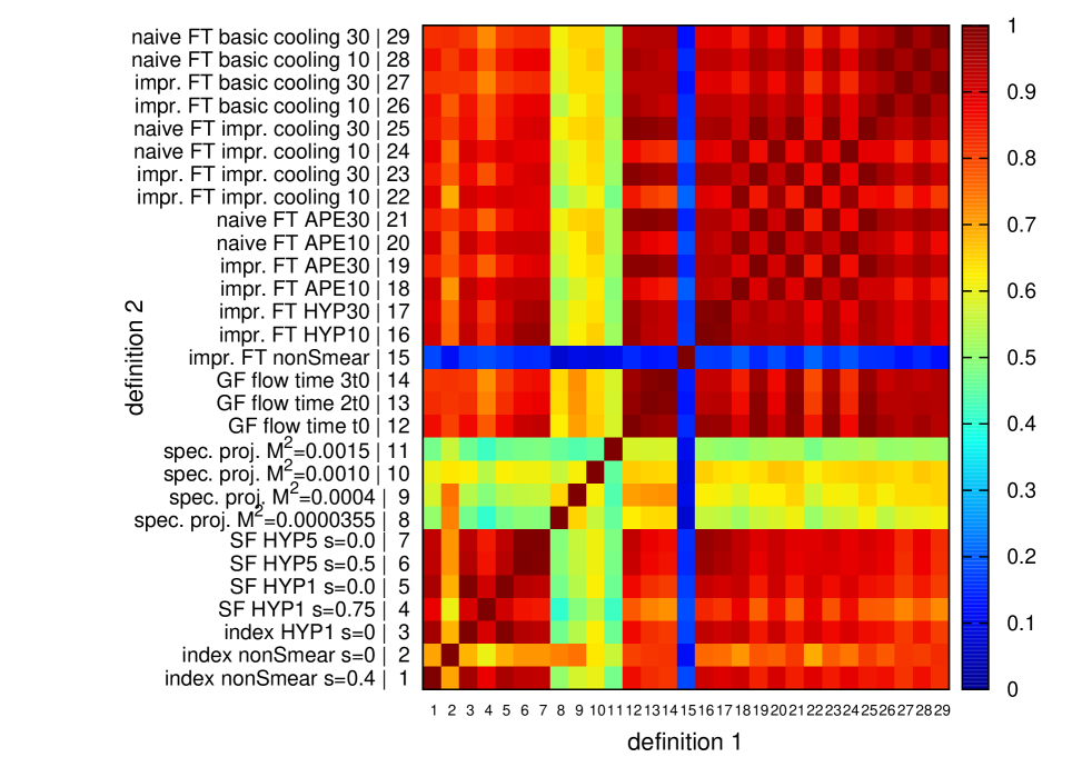
Figure 1: Correlation matrix between different definitions of the topological charge. Cool colours correspond to low correlations (blue: approx. no correlation), while warm colours denote large correlations (dark red: approx. perfect correlation). The employed definitions are all the ones contained in Tab. 1.

3.2 Correlation between different definitions

Our main result is the correlation matrix between different definitions of the topological charge, presented as a colour-coded graph in Fig. 1. We summarize here some conclusions.

• The general level of correlations between different definitions is very high – between 80% and nearly 100%. In particular, the topological charge extracted with the field theoretic definition but with different kinds of smoothing is typically 90-100% correlated.

• Exceptions to these rule are: field theoretic definition without any smoothing (where basically noise is extracted) and spectral projectors, for which the results are contaminated by the stochastic ingredient (correlation of 40-70% with other definitions).

• There is rather significant dependence of the index definition (extracted both from overlap and Wilson-Dirac spectral flow) on the mass parameter $s$. In certain cases, the correlation can drop even below 60%. This can be attributed to very bad locality properties of the overlap operator for some values of $s$, in particular $s=0$ (nonSmear) yields a very small decay rate of the overlap operator – for more details, see Ref. [20].

• The spectral projector definition shows a significant dependence on the parameter $M^{2}$. For the lowest considered $M^{2}$, the mode number is around 5, which means that not all zero modes are counted. For higher values of $M^{2}$ the correlation with other definitions increases up to some value where noise starts to dominate and the correlation again decreases.

• Gradient flow shows very similar results at different flow times ($t_{0}$, $2t_{0}$ and $3t_{0}$). Comparing to other definitions, better correlations are always observed with 30 rather than 10 steps of smearing or improved cooling, for both the naive and improved definition of the topological charge. This is not true for basic cooling, where correlations tend to be very similar for 10 and 30 cooling steps. This results from the underlying dependencies between gradient flow and cooling/smearing. We will comment more on this issue in the concluding part of this proceeding.

3.3 Topological susceptibility from different definitions

In Fig. 2, we show the results for the topological susceptibility for our test ensemble. The values of the susceptibility are for almost all methods within approx. 10% of the value $a\chi^{1/4}\approx 0.09$. Hence, although the values are not strictly compatible for different definitions, the differences can plausibly be attributed to cut-off effects. The values which are more than 10% off from 0.09 result from some flaws of the employed definitions: bad locality of the overlap Dirac operator (index nonSmear $s=0$), too small value of $M^{2}$ in spectral projectors or large UV fluctuations for the field theoretic definition on non-smoothed gauge fields.

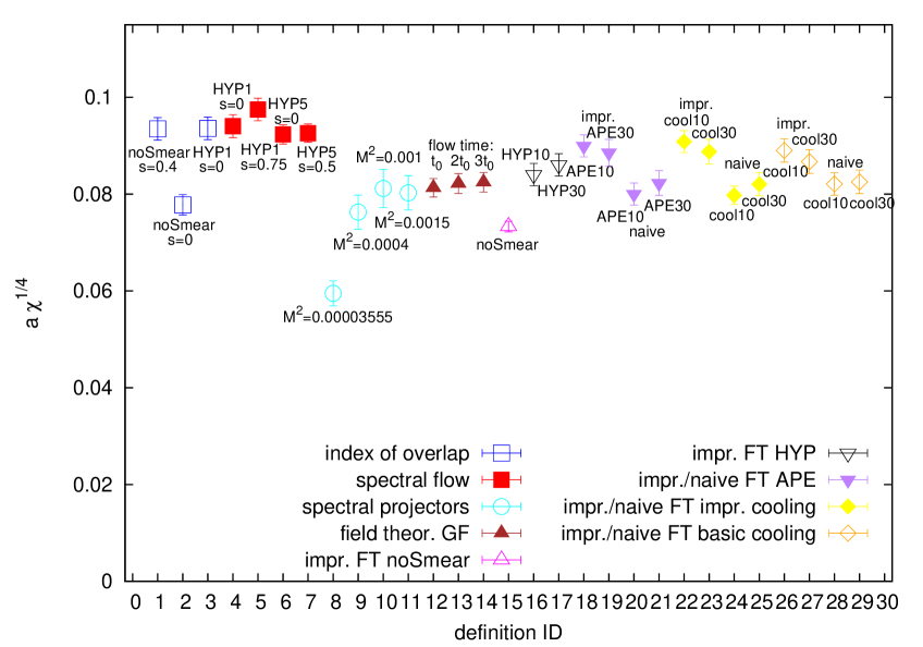
Figure 2: Topological susceptibility from different definitions. All the values are renormalized, except for HYP/APE, where the renormalization was not yet computed systematically, but the renormalization factor was estimated to be rather small, corresponding to a less than 5-percent shift upwards of $a\chi^{1/4}$. The employed definitions are all the ones contained in Tab. 1.

4 Conclusion

We presented preliminary results of our comparison of different definitions of the topological charge. We found that for all reasonable definitions (without easily identifiable flaws), the correlation between the values of the topological charge on our test ensemble is rather high and the values of the topological susceptibility are in a relatively small range.

In the near future, we plan to extend this investigation to finer lattice spacings to observe the presumed increase of correlation towards the continuum limit. Here, we would like to draw attention to an important aspect related to taking the continuum limit. This is rather unambiguous in the case of the fermionic definitions. However, for the field theoretic definition, one encounters the problem of matching the different lattice spacings. This can be done fully systematically if the smoothing procedure is gradient flow – one can consider the topological charge at a fixed flow time, e.g. $t_{0}$. A problem appears in the case of cooling/smearing, which can not be considered as rigorous procedures in the quantum field theoretic sense, since they are discrete. Nonetheless, to overcome this problem, one can perform the matching of cooling/smearing to gradient flow, thus defining the correspondence between flow time and the number of cooling/smearing steps. This has been done for the simplest case of gradient flow with the Wilson plaquette action and basic cooling [13], but it can be extended to more general cases. Thus, to investigate the increase of correlation towards the continuum limit, we plan to use a strategy to relate the number of cooling/smearing steps such that they correspond to the same flow time at different lattice spacings. We emphasize that only in this way the approach to the continuum limit can be considered to be reliable.

References

- [1] K. Cichy et al., in preparation.
- [2] P. Hasenfratz, V. Laliena and F. Niedermayer, Phys. Lett. B 427 (1998) 125 [hep-lat/9801021].
- [3] S. Itoh, Y. Iwasaki and T. Yoshie, Phys. Rev. D 36 (1987) 527.
- [4] L. Giusti and M. Lüscher, JHEP 0903 (2009) 013 [arXiv:0812.3638 [hep-lat]].
- [5] M. Lüscher and F. Palombi, JHEP 1009 (2010) 110 [arXiv:1008.0732 [hep-lat]].
- [6] K. Cichy, E. Garcia-Ramos and K. Jansen, JHEP 1402 (2014) 119 [arXiv:1312.5161 [hep-lat]].
- [7] M. Lüscher, JHEP 1008 (2010) 071 [arXiv:1006.4518 [hep-lat]].
- [8] M. Lüscher and P. Weisz, JHEP 1102 (2011) 051 [arXiv:1101.0963 [hep-th]].
- [9] B. Berg, Phys. Lett. B 104 (1981) 475.
- [10] Y. Iwasaki and T. Yoshie, Phys. Lett. B 131 (1983) 159.
- [11] M. Teper, Phys. Lett. B 162 (1985) 357.
- [12] E. M. Ilgenfritz, M. L. Laursen, G. Schierholz, M. Müller-Preussker and H. Schiller, Nucl. Phys. B 268 (1986) 693.
- [13] C. Bonati and M. D’Elia, Phys. Rev. D 89 (2014) 105005 [arXiv:1401.2441 [hep-lat]].
- [14] P. de Forcrand, M. Garcia Perez and I. O. Stamatescu, Nucl. Phys. B 499 (1997) 409 [hep-lat/9701012].
- [15] M. Albanese et al. [APE Collaboration], Phys. Lett. B 192 (1987) 163.
- [16] A. Hasenfratz and F. Knechtli, Phys. Rev. D 64 (2001) 034504 [hep-lat/0103029].
- [17] R. Frezzotti, P. A. Grassi, S. Sint and P. Weisz, JHEP 0108 (2001) 058 [arXiv:hep-lat/0101001].
- [18] R. Frezzotti and G. C. Rossi, JHEP 0408 (2004) 007 [arXiv:hep-lat/0306014].
- [19] K. Cichy, G. Herdoiza and K. Jansen, Nucl. Phys. B 847 (2011) 179 [arXiv:1012.4412 [hep-lat]].
- [20] K. Cichy, V. Drach, E. Garcia-Ramos, G. Herdoiza and K. Jansen, Nucl. Phys. B 869 (2013) 131 [arXiv:1211.1605 [hep-lat]].