Numerical simulations for the DRESDYN precession dynamo

Abstract

The next generation dynamo experiment currently under development at Helmholtz-Zentrum Dresden-Rossendorf (HZDR) will consist of a precessing cylindrical container filled with liquid sodium. We perform numerical simulations of kinematic dynamo action applying a velocity field that is obtained from hydrodynamic models of a precession driven flow. So far, the resulting magnetic field growth-rates remain below the dynamo threshold for magnetic Reynolds numbers up to ${\rm{Rm}}=2000$.

1 Introduction.

Planetary magnetic fields are generated by the dynamo effect, the process that provides for a transfer of kinetic energy from a flow of a conducting fluid into magnetic energy. Usually, it is assumed that these flows are driven by thermal and/or chemical convection but other mechanisms are possible as well. In particular, precessional forcing due to (regular) temporal changes of the orientation of Earth’s rotation axis has long been discussed as a complementary power source for the geodynamo [1, 2].

The basic principle of a fluid flow driven dynamo has been successfully demonstrated in three different experimental configurations, all of which using a more or less artificial flow driving [3, 4, 5]. Further progress is expected from present and future dynamo experiments like the Madison plasma dynamo experiment (MPDX, [6], the liquid metal spherical couette experiment at the University of Maryland [7] or the planned precession dynamo experiment that will be designed in the framework of the liquid sodium facility DRESDYN (DREsden Sodium facility for DYNamo and thermohydraulic studies, [8]).

Precession driven dynamos were found in simulations with a critical magnetic Reynolds number of the order of 1000 in a sphere [2], cylinder [9], spheroid [10], ellipsoid [11], and cube [12]. Experimentally, a precessing magnetohydrodynamical flow has been examined by R. Gans [13] in a cylinder with height $H=0.25~{}\rm{m}$, rotating with $\omega=60~{}\rm{Hz}$ and precessing with $\Omega=0.83~{}\rm{Hz}$ (thus yielding a precession ratio of $\Gamma=\Omega/\omega\approx 0.0138$). In these experiments an externally applied magnetic field was amplified by a factor of $\sim 3$ but the magnetic Reynolds number of this setup remains to small to cross the dynamo threshold.

In order to achieve the required large magnetic Reynolds number indicated by the above listed numerical studies, the scheduled precession dynamo experiment at HZDR must represent a greatly enlarged version of this previous setup making the construction of the experiment a challenge.

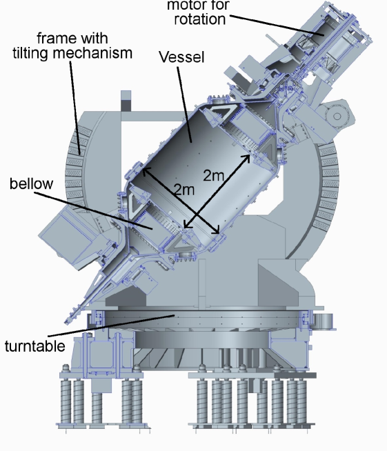
Figure 1: Sketch of the planned precession experiment. Diameter and height of the cylindrical container will be approximately $2~{}\rm{m}$. The precession angle can be varied from $\alpha=45^{\circ}$ to $\alpha=90^{\circ}$ (i.e. $\bvec{\omega}\perp\bvec{\Omega}$).

The setup will consist of a cylindrical container with height $H=2\,{\rm{m}}$ and radius $R=1\,{\rm{m}}$ filled with liquid sodium. The cylinder may rotate with a frequency of up to $\omega=10\,{\rm{Hz}}$ and precess with up to $\Omega=1\,{\rm{Hz}}$ (see left panel in figure 1). In contrast to previous dynamo experiments no internal blades, propellers or complex systems of guiding tubes will be used for the optimization of the flow properties.

2 Hydrodynamic flow properties.

A small scale water experiment is in operation in order to investigate the essential operation parameters for the liquid metal experiment, such as gyroscopic moments and associated load for the foundation, motor power consumption, typical flow pattern and flow amplitude (figure 2). This experiment is intended to supplement previous studies that were conducted as part of the French ATER experiment [14, 15, 16]. Most probably, the precession driven flow will be less suitable for dynamo action than the flow in highly optimized setups used in the dynamo experiments in Riga, Karlsruhe or Cadarache. In order to narrow suitable parameter regimes that may allow for dynamo action flow properties are estimated in dependence of precession angle $\alpha$, precession ratio $\Gamma=\Omega/\omega$ and Reynolds number ${\rm{Re}}=\omega R^{2}/\nu$. These properties will be included in kinematic simulations of the induction equation which are used to estimate the ability of different flow fields to provide for dynamo action.

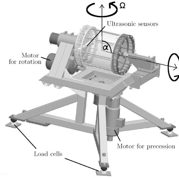
Figure 2: Sketch of the water model experiment. The dimensions of the cylinder are roughly six times smaller than the planned liquid metal experiment.

In the water experiment axial velocity profiles at different radial positions were measured using Ultrasonic Doppler Velocimetry (UDV). First results confirm observations of [14, 15] that precession provides an efficient flow forcing mechanism which yields bulk flow speeds of the order of one fifth to one third of the rotation speed of the container. In the liquid metal experiment this will correspond to flow velocities of up to $20~{}{\rm{m}}/{\rm{s}}$ so that a rather violent flow is expected. Based on the rotation speed of the cylinder at $\omega=10~{}{\rm{Hz}}$, and the diffusivity of liquid sodium ($\eta=0.08~{}{\rm{m}}^{2}/{\rm{s}}$ at $400~{}{\rm{K}}$), we expect magnetic Reynolds numbers of ${\rm{Rm}}=\omega R^{2}/\eta\sim 750$ which is rather close to the critical ${\rm{Rm}}$ reported by [9] from simulations of dynamo action in a precessing cylinder.

2.1 Transition to a chaotic state

The most striking feature in the water experiment is an abrupt transition at a critical precession ratio $\Gamma_{\rm{c}}\approx 0.07$ from a laminar state to a disordered chaotic behavior (see figure 3). The transition goes along with a sharp increase of the required motor power. The flow properties change significantly in the chaotic state with the simple $m=1$ Kelvin mode being suppressed, so that we expect a different regime for the dynamo as well.

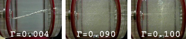
Figure 3: Snapshots of the precessing water cylinder at different precession rates. The container axis is aligned along the horizontal plane and the system precesses around the vertical axis ($\alpha=90^{\circ}$). Striking feature is the abrupt transition at critical precession ratio $\Gamma^{\rm{crit}}\approx 0.07$ from a laminar state (left panel) to more disordered chaotic behavior (central panel). For even larger $\Gamma$ the bulk fluid essentially is rotating around the precession axis (right panel).

2.2 Comparison with numerical simulations

For small Reynolds numbers the measurements are compared with simulations applying the code SEMTEX [17]. The code uses a spectral element method and a Fourier decomposition for the numerical solution of the Navier-Stokes equation which in the precessing frame reads:

$$\frac{\partial}{\partial t}\bvec{u}+(\bvec{u}\cdot\nabla)\bvec{u}+2(\bvec{\omega}+\bvec{\Omega})\times\bvec{u}=\nu\nabla^{2}\bvec{u}+\nabla\Phi$$ (1)

with the boundary condition $\bvec{u}=\bvec{\omega}\times\bvec{r}$. In equation (1) $\bvec{u}$ denotes the flow field, $\bvec{\omega}$ the rotation of the container, $\bvec{\Omega}$ the precession, $\nu$ the viscosity and $\Phi$ a reduced pressure that includes centrifugal forces. Note that equation (1) describes the precession problem in the so-called turntable frame in which the observer co-rotates with the precession looking at the rotating cylinder.

A comparison between numerical solutions and experimental measurements is shown in figure 4. For moderate precession ratio ($\Gamma=0.06$) the pattern and the amplitude of the velocity field are very similar (left column of figure 4). The agreement is worse for a larger precession ratio ($\Gamma=0.10$) where we observe a larger flow amplitude in the simulations compared to the experiment (right column).

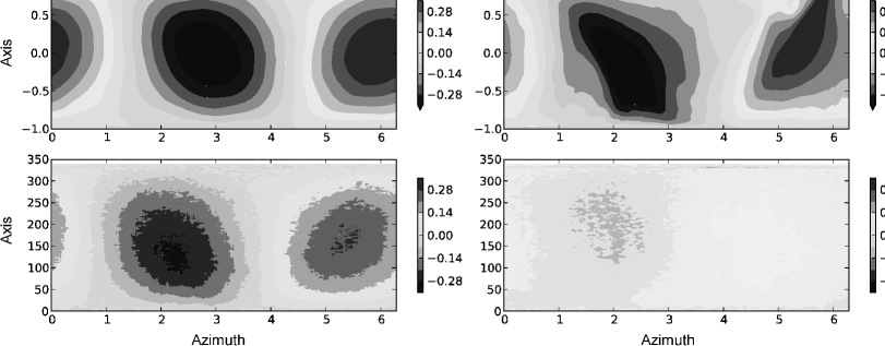
Figure 4: Comparison of the axial velocity at $r=0.74$ from hydrodynamic simulations (top row) and experimental measurements (bottom row). Left: $\Gamma=0.06$, right: $\Gamma=0.10$. The experimental data are measured at a rotation rate of $\omega=0.2~{}{\rm{Hz}}$ corresponding to ${\rm{Re}}\sim 33000$.

Main reason for these deviations is the transition to the chaotic state in the experiment (around $\Gamma\approx 0.07$) in which the fundamental $m=1$ Kelvin mode is suppressed. A vague evidence for such a transition in the simulations occurs only at significantly larger $\Gamma\approx 0.15$. This is indicated in figure 5 where the rotation axis of the bulk flow has changed its orientation from roughly parallel to the symmetry axis of the container (left panel) to a perpendicular direction (aligned with the precession axis, right panel).

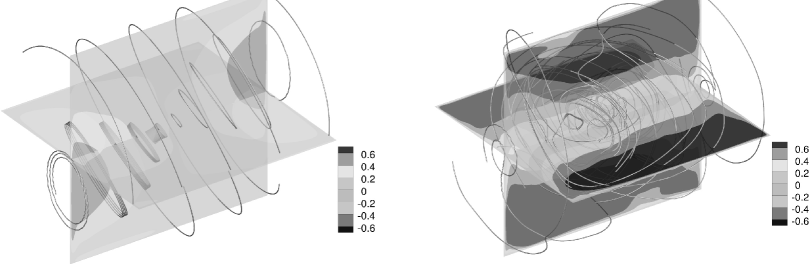
Figure 5: Streamlines from simulations with weak precessional forcing (left, $\Gamma=0.03$) and strong precessional forcing (right, $\Gamma=0.15$). Note the bulk flow rotating around the precession axis in the latter case.

The change of the orientation of the fluid axis is much less obvious (abrupt) in the simulation than in the water experiment which may be due to the much larger ${\rm{Re}}$ in the experiment.

3 Kinematic simulations of the induction equation.

In the following we concentrate on the more laminar regime with the main fluid rotation axis oriented (more or less) parallel to the container symmetry axis. We use different three dimensional velocity fields as an input for a kinematic solver for the magnetic induction equation which reads

$$\frac{\partial}{\partial t}\bvec{B}=\nabla\times(\bvec{u}\times\bvec{B}-\eta\nabla\times\bvec{B}).$$ (2)

In equation (2) $\bvec{B}$ denotes the magnetic flux density, $\bvec{u}$ the velocity field and $\eta$ the magnetic diffusivity. The numerical solution of equation (2) is computed using the numerical scheme presented in [18]. The resulting growth-rates $\gamma$ allow a quick estimation whether a given flow field is capable to drive a dynamo. The approach works well in the vicinity of the dynamo onset, but does not allow a consideration of non-linear effects like the magnetic back-reaction on the flow.

We use three different patterns for the velocity field. The simplest case (case I) makes use of analytic expressions that describe the fundamental inertial wave with azimuthal wave number $m=1$ (Kelvin mode). These solutions result from the linear in-viscid approximation of equation (1) and neglect the boundary layer flow as well as any non-linear interactions. The components of $\bvec{u}$ are explicitly given by [19, 20]

$$u_{r}\!\! \!\!=\!\! \!\!-\frac{1}{1-\omega_{n}^{2}}\!\left[\frac{dJ_{1}(2\lambda_{n}r)}{{\rm{d}}r}\!+\!\omega_{n}\frac{1}{r}J_{1}(2\lambda_{n}r)\right]\!\cos\!\left[k\pi\!\left(\frac{z}{H}\!+\!\frac{1}{2}\right)\right]\!\sin(\varphi\!+\!t)$$

$$u_{\varphi}\!\! \!\!=\!\! \!\!-\frac{1}{1-\omega_{n}^{2}}\!\left[\omega_{n}\frac{dJ_{1}(2\lambda_{n}r)}{{\rm{d}}r}\!+\!\frac{1}{r}J_{1}(2\lambda_{n}r)\right]\!\cos\!\left[k\pi\!\left(\frac{z}{H}\!+\!\frac{1}{2}\right)\right]\!\cos(\varphi\!+\!t)$$ (3)

$$u_{z}\!\! \!\!=\!\! \!\!\frac{k\pi}{h}J_{1}(2\lambda_{n}r)\sin\left[k\pi\left(\frac{z}{H}\!+\!\frac{1}{2}\right)\right]\sin(\varphi+t).$$

In equation (3) $J_{1}$ denotes the cylindrical Bessel-function of first kind, $H$ is the aspect ratio (height over radius), $k$ is the axial wavenumber, and $t$ is the time scaled by the forcing frequency $\omega$. $\lambda_{n}$ are the radial wave numbers which are computed from the dispersion relation:

$$\lambda\frac{{\rm{d}}J_{1}(\lambda)}{{\rm{d}}r}+\omega J_{1}(\lambda)=0$$ (4)

(which enforces the radial boundary conditions) and the eigenfrequencies $\omega_{n}$ result from the requirements imposed by the axial boundary conditions with integer axial wavenumber $k$ which leads to

$$\omega^{2}_{n}=1+\left(\frac{\lambda_{n}H}{k\pi}\right)^{2}$$ (5)

with $\lambda_{n}$ the $n$th root of (4). More elaborate expressions for the linear solutions of (1) that include the Ekman pumping and boundary layers are specified in [21]. However, in this study we are only interested on the critical magnetic Reynolds number required for the simplest possible flow pattern that can be excited by a precessional forcing. Hence, we normalize equations (3) so that $u_{\varphi}(r=R)=1$ and vary the magnetic diffusivity $\eta$ in order to change the magnetic Reynolds number defined by ${\rm{Rm}}=\omega R^{2}/\eta$. In a second step we might judge if this critical value corresponds to some reasonable flow amplitude. Any further effects resulting from boundary layers or higher azimuthal modes (triads) are ignored.

In order to estimate the impact of viscous boundary layers and non-linear interactions we apply flow fields resulting from the numerical simulations briefly described in section 2. We used data obtained from runs with precession ratio $\Gamma=0.1$ and ${\rm{Re}}=1500$ (case II) and with ${\rm{Re}}=6500$ (case III), respectively.

For ${\rm{Re}}=1500$ the flow is more or less stationary with a rather simple pattern that is very close to the analytic solutions for the fundamental $m=1$ Kelvin mode. Figure (6) shows the temporal behavior of the resulting magnetic energy density $E_{\rm{mag}}=\frac{1}{2\mu_{0}}\int\bvec{B}^{2}dV$ (left panel in 6). We do not find any growing solutions up to a magnetic Reynolds number ${\rm{Rm}}=2000$ and from the behavior of the corresponding growth rates it seems unlikely that a crossing of the dynamo threshold occurs within reasonable ${\rm{Rm}}$ (right panel in Figure 6).

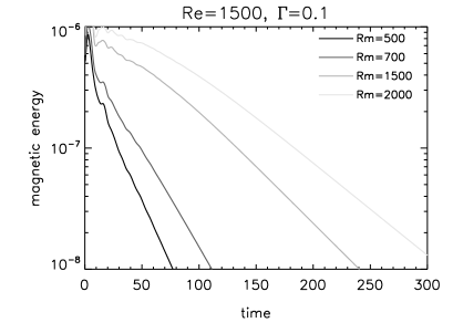
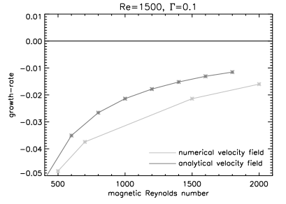
Figure 6: Left: temporal behavior of the magnetic energy for a velocity field obtained at ${\rm{Re}}=1500$ and $\Gamma=0.10$. Right: corresponding growth-rates of the fundamental dynamo eigenmode versus ${\rm{Rm}}$.

The dashed curve in the right panel of Figure 6 shows the growth-rates using the analytic expressions for the Kelvin modes given in Eq. (3). The behavior is quite similar to the growth-rates obtained from the simulations applying the flow field from the hydrodynamic simulations. Preliminary simulations with even larger ${\rm{Rm}}$ (not shown) indicate that indeed no crossing of the dynamo threshold occurs up to ${\rm{Rm}}=5000$.

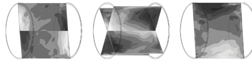
Figure 7: Snapshot of the flow components at ${\rm{Re}}=6500$. Note that the maximum flow is essentially concentrated close to the boundaries.

As a next step, we used a flow field obtained from hydrodynamic simulations at larger Reynolds number in order to capture the induction effects from a more time-dependent velocity field. We used a velocity field obtained at ${\rm{Re}}=6500$. At this value the flow is clearly time-dependent but still dominated by the $m=1$ mode (figure 7).

Again, we do not find any growing solutions for the magnetic field, however, the behavior of the growth-rates indicates a critical magnetic Reynolds number in the range of ${\rm{Rm}}=3000...4000$ (figure 8), which unfortunately would be far out of reach in the forthcoming dynamo experiment.

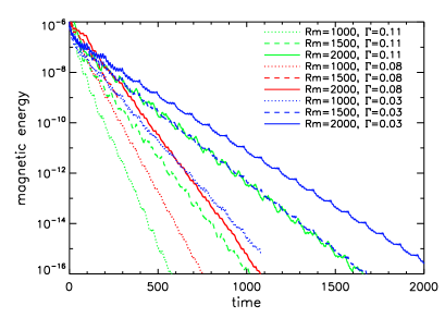
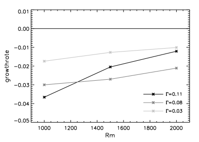
Figure 8: Left: temporal behavior of the magnetic field amplitude for a velocity field obtained at ${\rm{Re}}=6500$. Right: Corresponding growth-rates of the fundamental dynamo eigenmode versus ${\rm{Rm}}$.

4 Conclusion.

So far the kinematic simulations performed within this study did not show dynamo action. Reasons for this might be the simplistic structure of the flow which is close to the fundamental Kelvin mode in the low ${\rm{Re}}$ regime or restricted to regions close to the boundaries for larger ${\rm{Re}}$ (but still dominated by $m=1$). The behavior of the growth rates confirms the results from [22] where it was shown that inertial waves cannot drive a dynamo. However, our simulations were restricted to parameter regimes with quite low Reynolds number whereas the experiment will be characterized by ${\rm{Re}}\sim O(10^{8})$ and we expect an emergence of more complex flow structures for more realistic parameters.

Two promising candidates are already known from which we expect an improvement of the ability of the flow to drive a dynamo. The first are so-called triads consisting of the forced fundamental Kelvin mode and two free resonant inertial modes with larger azimuthal wavenumber. Such triadic resonances have repeatedly been observed in experiments and simulations of precessing flows [23, 24]. In a spherical geometry, a subclass of these modes have a close similarity to the columnar convection rolls that are responsible for dynamo action in geodynamo models and there is little reason to believe that this should not be the case with a precession driven flow field.

The second possibility relies on observations of cyclones in the French precession experiment ATER [16]. In that experiment large scale vortex-like structures emerge for intermediate precession ratios. These vortices are oriented along the rotation axis of the cylindrical container, and, depending on the parameter regime, their number varies between one and four (figure 9). The vortices are cyclonic, i.e., their sense of rotation is determined by the rotation orientation of the cylindrical container. We suspect that these vortices provide a significant amount of helicity, but so far, the axial dependence of their contribution and their interaction with the fundamental m=1 mode is unknown. Furthermore, cyclones were neither observed in the HZDR experiment (so far, no appropriate velocity measurements in a horizontal plane are available) nor in any simulations which probably must run at much higher Reynolds number in order to reveal these modes.

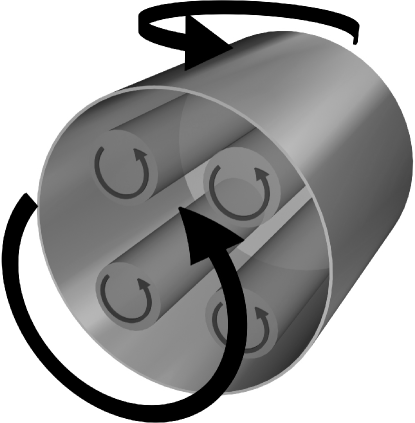
Figure 9: Idealized model for the cyclones observed in the ATER experiment [16].

The authors are grateful for support by the Helmholtz Allianz LIMTECH and kindly acknowledge discussions with C. Nore, J. Léorat and A. Tilgner.

References

- [1] W.V.R. Malkus. Precession of the Earth as the Cause of Geomagnetism. Science, vol. 160 (1968), pp. 259–264.
- [2] A. Tilgner. Precession driven dynamos. Phys. Fluids, vol. 17 (2005), 3, 034104.
- [3] A. Gailitis, O. Lielausis, S. Dement’ev, E. Platacis, A. Cifersons, G. Gerbeth, T. Gundrum, F. Stefani, M. Christen, H. Hänel, and G. Will. Detection of a Flow Induced Magnetic Field Eigenmode in the Riga Dynamo Facility. Phys. Rev. Lett., vol. 84 (2000), no. 19, pp. 4365–4368
- [4] R. Stieglitz and U. Müller. Experimental demonstration of a homogeneous two-scale dynamo. Phys. Fluids, vol. 13 (2001), pp. 561–564
- [5] R. Monchaux, M. Berhanu, M. Bourgoin, M. Moulin, P. Odier, J.-F. Pinton, R. Volk, S. Fauve, N. Mordant, F. Pétrélis, A. Chiffaudel, F. Daviaud, B. Dubrulle, C. Gasquet, L. Marié, and F. Ravelet. Generation of a Magnetic Field by Dynamo Action in a Turbulent Flow of Liquid Sodium. Phys. Rev. Lett., vol. 98 (2007), no. 4, 044502
- [6] C. M. Cooper, J. Wallace, M. Brookhart, M. Clark, C. Collins, W. X. Ding, K. Flanagan, I. Khalzov, Y. Li, J. Milhone, M. Nornberg, P. Nonn, D. Weisberg, D. G. Whyte, E. Zweibel, and C. B. Forest. The Madison plasma dynamo experiment: A facility for studying laboratory plasma astrophysics. Phys. Plasmas, vol. 21 (2014), no. 1, 013505
- [7] D. S. Zimmerman, S. A. Triana, H.-C. Nataf, and D. P. Lathrop. A turbulent, high magnetic Reynolds number experimental model of Earth’s core. J. Geophys. Res. (Solid Earth), vol. 119 (2014), pp. 4538-4557.
- [8] F. Stefani, S. Eckert, G. Gerbeth, A. Giesecke, T. Gundrum, C. Steglich, T. Weier, and B. Wustmann. DRESDYN – a new facility for MHD experiments with liquid sodium. Magnetohydrodynamics, vol. 48 (2012), no. 1, pp. 103–114.
- [9] C. Nore, J. Léorat, J.-L. Guermond, and F. Luddens. Nonlinear dynamo action in a precessing cylindrical container. Phys. Rev. E., vol. 84 (2011), no. 1, 016317.
- [10] C.C. Wu and P.H. Roberts. On a dynamo driven by topographic precession. Geophys. Astrophys. Fluid Dyn., vol. 103 (2009), no. 6, pp. 467–501.
- [11] J. Ernst-Hullermann, H. Harder, and U. Hansen. Finite volume simulations of dynamos in ellipsoidal planets. Geophys. J. Int., vol. 195 (2011), no. 3, pp. 1395–1405.
- [12] A. Krauze. Numerical modeling of the magnetic field generation in a precessing cube with a conducting melt. Magnetohydrodynamics, vol. 46 (2010), no. 3, pp. 271–280.
- [13] R.F. Gans. On hydromagnetic precession in a cylinder. J. Fluid Mech., vol. 45 (1971), pp. 111–130.
- [14] J. Léorat, F. Rigaud, R. Vitry, and G. Herpe. Dissipation in a flow driven by precession and application to the design of a MHD wind tunnel Magnetohydrodynamics, vol. 39 (2006), no. 3, pp. 321–326.
- [15] J. Léorat. Large scales features of a flow driven by precession. Magnetohydrodynamics, vol. 42 (2006), no. 2/3, pp. 143–151.
- [16] W. Mouhali, T. Lehner, J. Léorat, and R. Vitry. Evidence for a cyclonic regime in a precessing cylindrical container. Exp. Fluids, vol. 53 (2012), no. 6, pp. 1693–1700.
- [17] H. M. Blackburn and S. J. Sherwin. Formulation of a Galerkin spectral element-Fourier method for three-dimensional incompressible flows in cylindrical geometries. J. Comp. Phys., vol. 197 (2004), no. 2, pp. 759–778.
- [18] A. Giesecke, F. Stefani, and G. Gerbeth. Kinematic simulation of dynamo action by a hybrid boundary-element/finite-volume method. Magnetohydrodynamics, vol. 44 (2008), no. 3, pp. 237–252.
- [19] R. Manasseh. Distortions of inertia waves in a rotating cylinder forced near its fundamental mode resonance. J. Fluid Mech., vol. 265 (1994), pp. 345–370.
- [20] R. Manasseh. Nonlinear behaviour of contained inertia waves. J. Fluid Mech., vol. 315 (1996), pp. 151–173.
- [21] X. Liao and K. Zhang. On flow in weakly precessing cylinders: the general asymptotic solution. J. Fluid Mech., vol. 709 (2012), pp. 610–621.
- [22] W. Herreman and P. Lesaffre. Stokes drift dynamos. J. Fluid Mech., vol. 679 (2011), pp. 32–57.
- [23] S. Lorenzani and A. Tilgner. Inertial instabilities of fluid flow in precessing spheroidal shells. J. Fluid Mech., vol. 492 (2003), pp. 363–379.
- [24] R. Lagrange, P. Meunier, F. Nadal, and C. Eloy. Precessional instability of a fluid cylinder. J. Fluid Mech., vol. 666 (2011), pp. 104–145.