Optimal program-size complexity for self-assembly at temperature 1 in 3D

Abstract

Working in a three-dimensional variant of Winfree’s abstract Tile Assembly Model, we show that, for all $N\in\mathbb{N}$, there is a tile set that uniquely self-assembles into an $N\times N$ square shape at temperature 1 with optimal program-size complexity of $O(\log N/\log\log N)$ (the program-size complexity, also known as tile complexity, of a shape is the minimum number of unique tile types required to uniquely self-assemble it). Moreover, our construction is “just barely” 3D in the sense that it works even when the placement of tiles is restricted to the $z=0$ and $z=1$ planes. This result affirmatively answers an open question from Cook, Fu, Schweller (SODA 2011). To achieve this result, we develop a general 3D temperature 1 optimal encoding construction, reminiscent of the 2D temperature 2 optimal encoding construction of Soloveichik and Winfree (SICOMP 2007), and perhaps of independent interest.

1 Introduction

The simplest mathematical model of nanoscale tile self-assembly is Erik Winfree’s abstract Tile Assembly Model (aTAM) [14]. The aTAM extends classical Wang tiling [13] in that the former bestows upon the latter a mechanism for sequential “growth” of a tile assembly. Very briefly, in the aTAM, the fundamental components are un-rotatable, translatable square “tile types” whose sides are labeled with (alpha-numeric) glue “colors” and (integer) “strengths”. Two tiles that are placed next to each other bind if both the glue colors and the strengths on their abutting sides match and the sum of their matching strengths sum to at least a certain (integer) “temperature”. Self-assembly starts from a “seed” tile type, typically assumed to be placed at the origin, and proceeds nondeterministically and asynchronously as tiles bind to the seed-containing assembly one at a time. In this paper, we work in a three-dimensional variant of the aTAM in which tile types are unit cubes and growth proceeds in a noncooperative manner.

Tile self-assembly in which tiles may be placed in a noncooperative fashion is often referred to as “temperature 1 self-assembly”. Despite the arcane name, this is a fundamental and ubiquitous form of growth: it refers to growth from growing and branching tips in Euclidean space, where each new tile is added if it can bind on at least one side. Note that a more general form of cooperative growth, where some of the tiles may be required to bind on two or more sides, leads to highly non-trivial behavior in the aTAM, e.g., Turing universality [14] and the efficient self-assembly of $N\times N$ squares [1, 11] and other algorithmically specified shapes [12]. Doty, Patitz and Summers conjecture [6] that the shape or pattern produced by any 2D temperature 1 tile set that uniquely produces a final structure is “simple” in the sense of Presburger arithmetic [10]. However, their conjecture is currently unproven and it remains to be seen if noncooperative self-assembly in the aTAM can achieve the same computational and geometric expressiveness as that of cooperative self-assembly. In this paper, we specifically focus on a problem that is very closely related to that of finding the minimum number of distinct tile types required to self-assemble an $N\times N$ square, i.e., its tile complexity (or program-size complexity), at temperature 1.

The tile complexity of an $N\times N$ square at temperature 1 has been studied extensively. In 2000, Rothemund and Winfree [11] proved that the tile complexity of an $N\times N$ square at temperature 1 is $N^{2}$, assuming the final structure is fully connected, and at most $2N-1$, otherwise (they also conjectured that the lower bound, in general, is $2N-1$). A decade later, Manuch, Stacho and Stoll [9] established that, assuming no mismatches are present in the final assembly, the tile complexity of an $N\times N$ square at temperature 1 is $2N-1$. Shortly thereafter, and quite surprisingly, Cook, Fu and Schweller [5] showed that the tile complexity of an $N\times N$ square at temperature 1 is $O(\log N)$ if tiles are allowed to be placed in the $z=0$ and $z=1$ planes (here, an $N\times N$ square is actually a full 2D square in the $z=0$ plane with additional tiles above it in the $z=1$ plane).

Technically speaking, the aforementioned, just-barely-3D construction of Cook, Fu and Schweller is actually a general transformation that takes as input a 2D temperature 2 “zig-zag” tile set, say $T$, and outputs a corresponding 3D temperature 1 tile set, say $T^{\prime}$, that simulates $T$. In this transformation from $T$ to $T^{\prime}$, the tile complexity increases by $O(\log g)$, where $g$ is the number of unique north/south glues in the input tile set $T$. Since the number of north/south glues in the standard 2D aTAM base-$2$ binary counter is $O(1)$, Cook, Fu and Schweller use their transformation to produce several tile sets, which, when wired together appropriately and combined with “filler” tiles, self-assemble into an $N\times N$ square at temperature 1 in 3D with $O(\log N)$ tile complexity.

Of course, it is well-known that the tile complexity of an $N\times N$ square at temperature 2 is $O\left(\frac{\log N}{\log\log N}\right)$ [1], which, as Cook, Fu and Schweller point out in [5], is achievable using a zig-zag counter with an optimally-chosen base, say $b$, which satisfies $\frac{\log N}{\log\log N}<b<\frac{2\log N}{\log\log N}$, rather than in base $b=2$. However, using currently-known techniques, counting in base $b$ at temperature 2 requires having a tile set with $\Theta(b)$ unique north/south glues, whence the zig-zag transformation of Cook, Fu and Schweller cannot be used to get $O\left(\frac{\log N}{\log\log N}\right)$ tile complexity for an $N\times N$ square at temperature 1 in 3D. Moreover, the optimal encoding scheme of Soloveichik and Winfree [12] and the base conversion technique of Adleman et. al. [1] do not work correctly at temperature 1 and they also cannot be simulated by the Cook, Fu and Schweller construction without an $\Omega\left(\frac{\log N}{\log\log N}\right)$ blowup in tile complexity. Thus, Cook, Fu and Schweller, at the end of section 4.4 in [5], pose the following question: is it possible to achieve the tile complexity bound of $O\left(\frac{\log N}{\log\log N}\right)$ for an $N\times N$ square at temperature $1$ in 3D?

In Theorem 4.1, the main theorem of this paper, we answer the previous question in the affirmative, i.e., we prove that the tile complexity of an $N\times N$ square at temperature 1 in 3D is $O\left(\frac{\log N}{\log\log N}\right)$ (in our construction, tiles are placed only in the $z=0$ and $z=1$ planes of $\mathbb{Z}^{3}$). Our tile complexity matches a corresponding lower bound dictated by Kolmogorov complexity (see [7] for details on Kolmogorov complexity), which was established by Rothemund and Winfree in 2000, and holds for all “algorithmically random” values of $N$ [11]. Thus, our construction yields optimal tile complexity for the self-assembly of $N\times N$ squares at temperature 1 in 3D, for all algorithmically random values of $N$. To achieve optimal tile complexity, we adapt the optimal encoding technique of Soloveichik and Winfree [12] (which, itself, is based on the base-conversion scheme of [1]) to work at temperature 1 in 3D. Our 3D temperature 1 optimal encoding technique, described in Section 3, is perhaps of independent interest.

2 Definitions

In this section, we give a brief sketch of a $3$-dimensional version of Winfree’s abstract Tile Assembly Model.

2.1 3D abstract Tile Assembly Model

Let $\Sigma$ be an alphabet. A $3$-dimensional tile type is a tuple $t\in(\Sigma^{*}\times\mathbb{N})^{6}$, e.g., a unit cube with six sides listed in some standardized order, each side having a glue $g\in\Sigma^{*}\times\mathbb{N}$ consisting of a finite string label and a non-negative integer strength. In this paper, all glues have strength $1$. There is a finite set $T$ of $3$-dimensional tile types but an infinite number of copies of each tile type, with each copy being referred to as a tile.

A $3$-dimensional assembly is a positioning of tiles on the integer lattice $\mathbb{Z}^{3}$ and is described formally as a partial function $\alpha:\mathbb{Z}^{3}\dashrightarrow T$. Two adjacent tiles in an assembly bind if the glue labels on their abutting sides are equal and have positive strength. Each assembly induces a binding graph, i.e., a grid graph whose vertices are (positions of) tiles and whose edges connect any two vertices whose corresponding tiles bind. If $\tau$ is an integer, we say that an assembly is $\tau$-stable if every cut of its binding graph has strength at least $\tau$, where the strength of a cut is the sum of all of the individual glue strengths in the cut.

A $3$-dimensional tile assembly system (TAS) is a triple $\mathcal{T}=\left(T,\sigma,\tau\right)$, where $T$ is a finite set of tile types, $\sigma:\mathbb{Z}^{3}\dashrightarrow T$ is a finite, $\tau$-stable seed assembly, and $\tau$ is the temperature. In this paper, we assume that $|{\rm dom}\;{\sigma}|=1$ and $\tau=1$. An assembly $\alpha$ is producible if either $\alpha=\sigma$ or if $\beta$ is a producible assembly and $\alpha$ can be obtained from $\beta$ by the stable binding of a single tile. In this case we write $\beta\to_{1}^{\mathcal{T}}\alpha$ (to mean $\alpha$ is producible from $\beta$ by the binding of one tile), and we write $\beta\to^{\mathcal{T}}\alpha$ if $\beta\to_{1}^{\mathcal{T}^{*}}\alpha$ (to mean $\alpha$ is producible from $\beta$ by the binding of zero or more tiles). When $\mathcal{T}$ is clear from context, we may write $\to_{1}$ and $\to$ instead. We let $\mathcal{A}\left[\mathcal{T}\right]$ denote the set of producible assemblies of $\mathcal{T}$. An assembly is terminal if no tile can be $\tau$-stably bound to it. We let $\mathcal{A}_{\Box}\left[\mathcal{T}\right]\subseteq\mathcal{A}\left[\mathcal{T}\right]$ denote the set of producible, terminal assemblies of $\mathcal{T}$.

A TAS $\mathcal{T}$ is directed if $\left|\mathcal{A}_{\Box}\left[\mathcal{T}\right]\right|=1$. Hence, although a directed system may be nondeterministic in terms of the order of tile placements, it is deterministic in the sense that exactly one terminal assembly is producible. For a set $X\subseteq\mathbb{Z}^{3}$, we say that $X$ is uniquely produced if there is a directed TAS $\mathcal{T}$, with $\mathcal{A}_{\Box}\left[\mathcal{T}\right]=\{\alpha\}$, and ${\rm dom}\;{\alpha}=X$.

For $N\in\mathbb{N}$, we say that $S^{3}_{N}\subseteq\mathbb{Z}^{3}$ is a 3D $N\times N$ square if $\{0,\ldots,N-1\}\times\{0,\ldots,N-1\}\times\{0\}\subseteq S^{3}_{N}\subseteq\{0,\ldots,N-1\}\times\{0,\ldots,N-1\}\times\{0,1\}$. In other words, a 3D $N\times N$ square is at most two 2D $N\times N$ squares, one stacked on top of the other.

In the spirit of [11], we define the tile complexity of a 3D $N\times N$ square at temperature $\tau$, denoted by $K^{\tau}_{3DSA}(N)$, as the minimum number of distinct 3D tile types required to uniquely produce it, i.e., $K^{\tau}_{3DSA}(N)=\min\left\{n\;\left|\;\mathcal{T}=\left(T,\sigma,\tau\right),\left|T\right|=n\textmd{ and }\mathcal{T}\textmd{ uniquely produces }S^{3}_{N}\right.\right\}$.

2.2 Notation for figures

In the figures in this paper, we use big squares to represent tiles placed in the $z=0$ plane and small squares to represent tiles placed in the $z=1$ plane. A glue between a $z=0$ tile and $z=1$ tile is denoted as a small black disk. Glues between $z=0$ tiles are denoted as thick lines. Glues between $z=1$ tiles are denoted as thin lines.

3 Optimal encoding at temperature 1

A key problem in algorithmic self-assembly is that of providing input to a tile assembly system (e.g., the size of a square, the input to a Turing machine, etc.). In real-world laboratory implementations, as well as theoretical constructions, input to a tile system is typically provided via a (possibly large) collection of “hard-coded” seed tile types that uniquely assemble into a convenient “seed structure,” such as a line of tiles that encodes some input value. Unfortunately, in practice, it is more expensive to manufacture different types of tiles than it is to create copies of each tile type. Thus, it is critical to be able to provide input to a tile system using the smallest possible number of hard-coded seed tile types.

Consider the problem of constructing a tile set that uniquely self-assembles from a single seed tile into a “seed row” that encodes an $n$-bit binary string, say $x$. The most straightforward way to do this is to construct a set of $n$ unique tile types that deterministically assemble into a line of tiles of length $n$, where each tile in the line represents a different bit of $x$. This simple construction encodes one bit of $x$ per tile, whence its tile complexity is $O(n)$. Note that, in this example, each tile type is an element of a set of size $n$, yet each tile type encodes only 1 bit of information, instead of the optimal $O(\log n)$ bits. Is there a more efficient encoding construction?

The optimal encoding constructions of Adleman et al. [1], and Soloveichik and Winfree [12] are more efficient methods of encoding input to a tile set. These constructions are based on the idea that each seed row tile type should encode $k=O(\log n)$ bits – instead of a single bit – of $x$, which means that $O(n/\log n)$ unique tile types suffice to uniquely self-assemble into a seed row that encodes the bits of $x$. Unfortunately, now the bits of $x$ are no longer conveniently represented in distinct tiles. Fortunately, if $k$ is chosen carefully, then it is possible to use a tile set of size $O(n/\log n)$ to “extract” the bits of $x$ into a more convenient one-bit-per-tile representation, which can be used to seed a binary counter or a Turing machine simulation.

Up until now, all known optimal encoding constructions (e.g., [1, 12]) required cooperative binding (that is, temperature $\tau\geq 2$). In what follows, we propose an optimal encoding construction (based on the construction of Soloveichik and Winfree [12]) that works at temperature $\tau=1$ and is “just barely” 3D, i.e., tiles are only placed in the $z=0$ and $z=1$ planes.

3.1 Setup

Let $x=x_{n-1}x_{n-2}...x_{1}x_{0}$ be the input string, where $x_{i}\in\{0,1\}$. Let $m=\left\lceil n/k\right\rceil$, where $k$ is the smallest integer satisfying $2^{k}\geq n/\log n$. We write $x=w_{0}w_{1}...w_{m-2}w_{m-1}$, where each $w_{i}$ is a $k$-bit block. Note that $w_{0}$ is padded to the left with leading 0’s, if necessary. In the figures in this section, a green tile represents a starting point for some portion of an assembly sequence, and a red tile represents an ending point.

3.2 Overview of the construction

We extract each of the $m$ $k$-bit blocks within a roughly rectangular region of space of width $O(k)$ and height $O(m)$. We refer to this region of space as a “block extraction region” (or simply “extraction region”). For each $0\leq i<m$, we extract block $w_{i}$ in extraction region $i$. Each extraction region, other than the first and last ones, assembles via a series of gadgets (small groups of tiles that carry out a specific task).

We encode the $k$ bits of a $k$-bit block as a series of geometric bumps along a path of tiles that makes up the top border of an extraction region. A bump in the $z=0$ plane represents the bit 0 and a bump in the $z=1$ plane represents the bit 1. The end result of our construction is an assembly in which each bit of $x$ is encoded in its own bit-bump (see Figure 10 for an example).

We extract the $k$-bit blocks in order, starting with the first block $w_{0}$, which represents the most significant bits of $x$. Normally, to carry out this sort of activity at temperature 1 (i.e., to enforce the ordering of tile placements), one has to encode the order of placement directly into the glues of the tiles. However, for our construction, this would essentially mean encoding the number of the block that is being extracted into the glues of the tiles that fill in its extraction region. Unfortunately, doing so, at least in the most straightforward way, results in an increase in tile complexity from the optimal $O(n/\log n)$ to $\Omega(n^{2}/\log^{2}n)$.

Therefore, in our construction, we encode the number of the block that is being extracted as a geometric pattern along a vertical path of tiles that runs along the right side of each extraction region. We call this special geometric pattern the “block number.” Then we use a special gadget called the “block-number gadget” to search for this pattern.

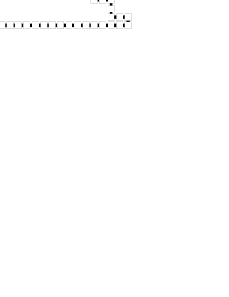
Figure 1: The perimeter of the first extraction region is hard-coded to self-assemble like this. In this example, the four bumps along the top (from left to right) represent the bits 1, 0, 0 and 1, respectively. The green tile (bottom tile in the penultimate column) is the single seed tile for our entire optimal encoding construction.

Within an extraction region, the block number determines which block gets extracted next. Basically, the path along which the block number is encoded blocks the placement of $m-1$ special tiles, each of which tries to initiate the extraction of a particular $k$-bit block. We call these special tiles “extraction tiles.” Since the first extraction region is hard-coded (see below), the first block does not have an extraction tile associated with it. Within any given extraction region, exactly one extraction tile will not be blocked. The one extraction tile that is not blocked by the block number gadget will initiate the extraction of the $k$ bits of the block to which it corresponds.

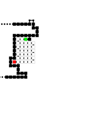
(a)

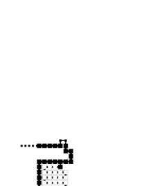
(b)

(c)

(d)

Figure 2: This sequence of figures shows how the position of the block number is found. The black tiles correspond to tiles of the previous extraction region.

In our construction, we hard-code the assembly of the first and last extraction regions. What this means is that, in each of these extraction regions, a single-tile-wide path assembles the perimeter and then we use a filler tile to fill in the interior. For this step, it is crucial to first assemble the perimeter of the extraction region and then use a filler tile to tile the interior. Note that, if one were to uniquely tile every location in the first (or last) extraction region, then the tile complexity of the construction would be $\Omega(mk)$, which is not optimal. Tiling the perimeter of either the first or last extraction region can be done with $O(m+k)$ unique tile types (see Figure 1 for the example of the first extraction region).

All extraction regions other than the first and last ones are constructed using a general set of gadgets. In the second extraction region, which is the first generally-constructed extraction region, the block-number gadget determines that $w_{1}$ is the next block to be extracted by “searching” for the block number position. When the block number is found, a path of tiles, initiated by the extraction tile for $w_{1}$, is allowed to assemble (see Figure 2 for an example of this process). In general, for extraction region $i$, for all $1\leq i<m-1$, the path along which the block number is encoded geometrically hinders the placement of all extraction tiles that correspond to blocks $w_{1},...,w_{i-1},w_{i+1},...,w_{m-2}$.

Each extraction tile initiates the extraction of the $k$-bit block to which it corresponds (see Figure 3). We use a set of “bit-extraction” gadgets to extract a $k$-bit block into a one-bit-per-bump representation (the bit extraction gadgets are collectively referred to as the “extraction gadget”). Our bit extraction gadgets are basically 3D, temperature 1 versions of the “extract bit” tile types in Figure 5.7a of [12].

Figure 3: The bits of the current block are represented as bumps along the top of the extraction region that is currently being assembled.

After a block, say $w_{i}$, for $i>0$, is extracted, the block number is geometrically “incremented”, i.e., its position is translated up by a small constant amount (notice the position of the white “hook” at the bottom of Figure 3). We do this in two phases. First, the current position of the block number is found and then it is incremented and translated. Figure 4 shows how the current position of the block number is detected using a zig-zag path of tiles. Figure 5 shows how the current position of the block number is geometrically incremented.

Figure 4: A path of tiles searches for the block number, represented by a notch in a previous portion of the assembly. The red tile “knows” that it found the position of the block number because it was allowed to be placed.

Figure 5: The block number is geometrically incremented. The green tile “jumps” over the previous gadget that found the position of the block number and grows a hook of tiles to represent the updated block number. Notice that the new hook of tiles is two tiles higher than the previous hook (shown in black), which corresponds to the two rows of tiles that each block takes up in the block-number gadget.

After the block number has been updated, a series of gadgets geometrically propagate the position of the block number to the right through the remainder of extraction region $i$ so that it is advertised to extraction region $i+1$. This is shown in Figures 6 and 7. Technically, we geometrically propagate the block number position through the rest of the extraction region using a series of gadgets. Logically, however, we do this in two phases, which are iterated: “up” propagation and “down” propagation.

Figure 6: A series of gadgets geometrically propagate the position of the block number through the rest of the extraction region. This figure shows two of the gadgets. The first one assembles upward until it is blocked by a previous portion of the assembly. The second one assembles horizontally and to the right as it jumps over the top row of the previous gadget.

Figure 7: The position of the block number is propagated through the rest of the extraction region.

The “up” propagation phase grows from the position of the block number up to (and is blocked by) a previous portion of the assembly. This is shown in Figure 6. The “down” propagation phase grows from the top of the previous (up) propagation phase back down to the position of the block number. The upward growth of each up propagation phase is blocked in the $z=0$ plane but not in the $z=1$ plane. However, this is switched for the last up propagation phase. In other words, the last up propagation phase may continue its upward growth, which signals the end of the extraction region, but its $z=1$ growth is blocked. In Figure 8, the last up propagation phase is allowed to continue its upward growth in the $z=0$ plane.

Figure 8: The last up propagation phase detects when it has reached the end of the extraction region and initiates a perimeter gadget (see Figure 9) that will fill in the bottom row of the current extraction region before the next extraction region begins.

The last up propagation phase initiates the assembly of a special gadget that fills in the bottom row of the current extraction region before the next extraction region begins. The reason we do this is to ensure that, when the entire extraction process is done (i.e., when all $n$ bits have been extracted into a one-bit-per-bump representation), the bottom row of the assembly is completely filled in. Figure 9 shows an example of how this gadget tiles the remaining perimeter of an extraction region. Note that the tile complexity of this gadget is the size of the perimeter of an extraction region, i.e., $O(m)$.

Figure 9: The bottom row of the extraction region is tiled by a special gadget with $O(m)$ tile complexity. After the bottom row of the extraction region is tiled, the next extraction region is initiated. Notice that the red tile in this figure belongs to the same row of tiles as the red tile in Figure 1 but the position of the block number has moved up, which means the extraction tile for the next block (in this case, $w_{2}$) will be allowed to assemble and all other extraction tiles will be blocked.

The final extraction region, like the initial extraction region, is hard-coded to assemble its perimeter via a single-tile-wide path. The tiles that comprise the final extraction region “know” to stop the extraction process and possibly initiate the growth of some other logical component of a larger assembly, e.g., a binary counter or a Turing machine simulation in which the extracted bits of $x$, along the top of each of the $m$ extraction regions, are used as input.

The end result of our optimal encoding construction is a roughly rectangular assembly of tiles with height $O(m)$ and width $O(n)$, where each bit of $x$ is encoded as a bump (either in the $z=0$ or $z=1$ plane) along the top of the rectangle, with four “spacer” tiles to the left and right of each bit-bump. Figure 10 shows the result of our optimal encoding construction with four extraction regions. Complete details for this construction are in the appendix (see Section 6.1).

Figure 10: This is an example of our optimal encoding construction using $n=16$ and $k=4$. Note that this does not correspond to an actual instance of our optimal encoding construction because if $n=16$, then the smallest value of $k$ satisfying $2^{k}\geq n/\log n$ is $k=2$. The bit string encoded along the top is $1001001100111000$. All of the empty spaces in the $z=0$ plane are filled in with the same filler tile.

3.3 Tile complexity

To establish the tile complexity bound of $O(n/\log n)$ for our construction, we use the following technical lemma.

Lemma 3.1.

Let $1<n\in\mathbb{Z}^{+}$ and $m=\left\lceil n/k\right\rceil$, where $k$ is the smallest integer satisfying $2^{k}\geq n/\log n$. Then $m=O(n/\log n)$.

Proof.

Assume the hypothesis. First, note that, by our choice of $k$, $2^{k}<2n/\log n$. Then we have

$$m = \left\lceil\frac{n}{k}\right\rceil\leq\left\lceil n/\log(n/\log n)\right\rceil=\left\lceil n/(\log n-\log\log n)\right\rceil<\left\lceil n/(\log n-(\log n)/2)\right\rceil$$

$$\leq 2n/\log n+1\leq 2n/\log n+n/\log n=3n/\log n=O(n/\log n)$$

∎

The tile complexity of our construction is the sum of the tile complexities of all of the gadgets that assemble all extraction regions.

We will first analyze the tile complexity of the extract bit gadgets. Recall that these gadgets convert a $k$-bit binary string, encoded as a strength-$1$ glue, into a one-bit-per-bump representation. The first bit-extraction gadget accepts a $k$-bit binary string, converts the most significant bit of the block into the appropriate bump and then outputs a $(k-1)$-bit binary string. The latter is the input for the second bit-extraction gadget. This process is iterated $k$ times (once for each bit). For a given $n$ and our choice of $k$ (as described above), the number of distinct extract bit gadgets needed in our construction can be computed as:

$$2\left(\left|\{0,1\}^{0}\right|+\left|\{0,1\}^{1}\right|+\cdots+\left|\{0,1\}^{k-1}\right|\right) = 2\left(1+2+\cdots+2^{k-1}\right)$$

$$= 2\left(2^{k}-1\right)<2\cdot 2^{k}<4n/\log n=O\left(n/\log n\right)$$

Since each bit-extraction gadget is comprised of $O(1)$ unique tile types, the total tile complexity for the extraction gadgets is $O(n/\log n)$.

It is easy to see that all other gadgets in our construction can be implemented using $O(m)$ unique tile types (see Section 6.1 for details). Thus, by Lemma 3.1, the tile complexity of our construction is $O(n/\log n)$, which is optimal for all algorithmically random values of $n$.

4 Optimal self-assembly of squares at temperature 1 in 3D

In this section, we describe how to use our 3D temperature 1 optimal encoding construction to prove the following theorem.

Theorem 4.1.

$K^{1}_{3DSA}(N)=O\left(\frac{\log N}{\log\log N}\right)$.

Proof.

Our proof is constructive. Figure 11a shows how we build an $N\times N$ square using two counters C1 and C2 and two filler regions F1 and F2. Counter C1 is a zig-zag counter whose construction is described in the appendix (see Section 6.2). Counter C2 is identical to C1 after a 90-degree clockwise rotation. Each counter is seeded with a value produced by an optimal encoding region (OER for short). The full construction for F1 is depicted in Figure 12. F2 is a smaller, mirror-image of F1 with minor modifications to properly connect all of the pieces of the square. Both F1 and F2 are essentially squares, except for two hooks needed to stop the horizontal and vertical growths of each filler region, namely, one eight-tile hook encroaching on and another one-tile hook protruding from each filler region (see Figure 12). These hooks require simple modifications of the OER regions (see Figure 11b) that are all located in the hard-coded (i.e., first and last) block extracting regions of OER1 and OER2. Note that F1 is also missing a two-tile wide rectangle region on its left that is used up by the vertical connector that initiates the assembly of OER2 immediately after the assembly of C1 terminates. Figure 11c shows the assembly sequence for the whole square, while Figure 11b zooms in on the region of the square where OER1, F1, OER2 and F2 all interact.

(a) Overall square construction.

(b) Detail of the region of the square where OER1, F1, OER2 and F2 meet.

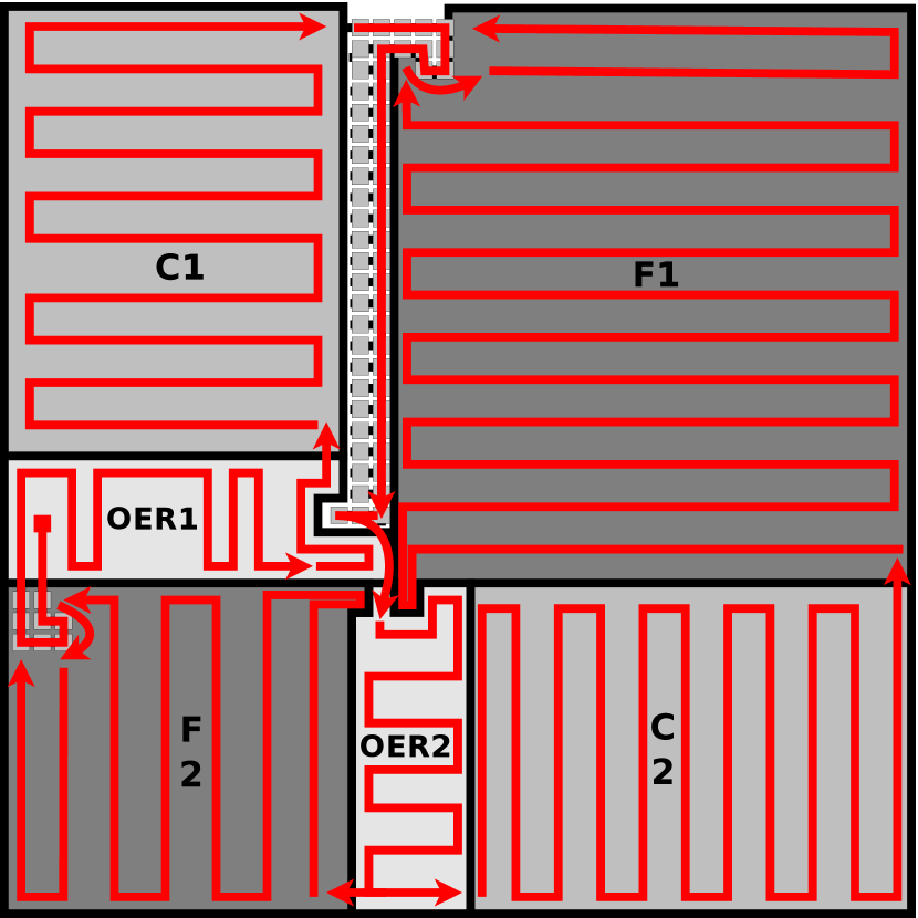
(c) The assembly sequence for the whole square is shown with red arrows starting from the seed tile (the red square located in OER1). The central region in this sub-figure is shown in more detail in Figure 11b to the left.

Figure 11: Construction of an $N\times N$ square, where $m$ is $O\left(\frac{\log N}{\log\log N}\right)$. The counters C1 and C2 (in medium gray) are identical up to rotation. So are their seed rows, each of which is the output of an optimal extraction region (OER1 and OER2, respectively, in light gray). F1 and F2 (in dark gray) are filler regions.

The gray tiles in this figure do not belong to F1. They are all added to the $N\times N$ square assembly before F1 starts assembling and they determine the height and width of F1, both of which are adjustable in the following way:

• The height of F1 is always a multiple of four (i.e., the total height of each pink plus red gadget), plus the number of purple rows at the top, which can be hard-coded to any value in $\{1,2,3,4\}$, together with a corresponding increase in the height of the top-left (gray) hook.

• The width of F1 is always a multiple of two (i.e., the width of each pink gadget) plus the width of each orange gadget, which is either three (by deleting the column occupied by the white tiles) or four (as shown).

Therefore, this construction gives us two knobs, namely the number of purple rows and the width of the orange gadget, to assemble filler regions of any height and width, respectively.

Figure 12: Detailed construction for the F1 filler region in Figure 11

First, we compute the tile complexity of our construction as the sum of the tile complexities of all of the components that make up the $N\times N$ square. Let $n=\lceil\log N\rceil$. If $k$ denotes the smallest integer satisfying $2^{k}\geq n/\log n$ and $m$ is defined as $\lceil n/k\rceil$, then the tile complexity of each OER is $O(n/\log n)$, as proved in Section 3.3. Furthermore, the tile complexity of each binary counter is $O(1)$ (see Section 6.2). Finally, the tile complexity of each filler region is $O(1)$, since each colored gadget in Figure 12 has tile complexity $O(1)$. Therefore, the tile complexity of our square construction is dominated by that of the OERs and is therefore $O(\frac{n}{\log n})=O\left(\frac{\log N}{\log\log N}\right)$.

Second, we need to prove that our tile system is directed and does produce an $N\times N$ square. The assembly sequence depicted in Figure 11c demonstrates that our tile system uniquely produces a square. To make sure that this square has width $N$, we need to pick the initial value $i$ of the counters and adjust the size of the filler regions as follows. The width of OER1, C1 and F2 in our construction, and thus also the height of OER2, C2 and F2 is $6n+4$. The height of OER1, and thus also the width of OER2, is $2m+7$ (see, for example, Figure 10). Therefore, the height of C1 (and thus also the width of C2) must be equal to $N-(2m+7+6n+4)=N-2\left\lceil\frac{\lceil\log N\rceil}{k}\right\rceil-6\lceil\log N\rceil-11$. Let us denote this value by $h(N)$. Our construction in Section 6.2 gives us two knobs to control the height of any $n$-bit counter: the initial value $i$ of the counter and the number $r$ of rooftop rows, where $r\in\{1,2,3,4\}$. Since each value from $i$ to the final value of the counter $2^{n}-1$ (inclusive) takes up four rows of tiles, we must have $\lfloor\frac{h(N)}{4}\rfloor=2^{n}-i$ and $r=1+h(N)\bmod 4$. Therefore, for both C1 and C2, the initial value of the counter is $2^{n}-\lfloor\frac{h(N)}{4}\rfloor$. Finally, the correct height and width of F1 are obtained by setting the two knobs described in Figure 12 to $1+(2m+7+h(N)-1)\bmod 4$ and $4-(2m+7+h(N)-2)\bmod 2$, respectively. Similarly, the correct height and width of F2 are obtained by setting the second knob to $4-(6n+4)\bmod 2$ and the first knob to $1+(6n+4-1)\bmod 4$. ∎

5 Conclusion

In this paper, we developed a 3D temperature 1 optimal encoding construction, based on the 2D temperature 2 optimal encoding construction of Soloveichik and Winfree [12]. We then used our construction to answer an open question of Cook, Fu and Schweller [5], namely, we proved that $K^{1}_{3DSA}(N)=O\left(\frac{\log N}{\log\log N}\right)$, which is the optimal tile complexity for all algorithmically random values of $N$.

We propose a future research direction as follows. Consider a generalization of the aTAM, called the two-handed [2] (a.k.a., hierarchical [3], q-tile, multiple tile [4], polyomino [8]) abstract Tile Assembly Model (2HAM). A central feature of the 2HAM is that, unlike the aTAM, it allows two “supertile” assemblies, each consisting of one or more tiles, to bind. In the 2HAM, an assembly of tiles is producible if it is either a single tile, or if it results from the stable combination of two other producible assemblies. Now define the quantity $K^{\tau}_{3D2SA}(N)$, as the minimum number of distinct 3D tile types required to uniquely produce it in the 2HAM at temperature $\tau$. An interesting problem would be to determine if $K^{1}_{3D2SA}(N)=O\left(\frac{\log N}{\log\log N}\right)$.

6 Appendix

In this section, we provide details on two of our constructions, namely the optimal encoding and the zig-zag counter, that did not fit in the main body of the paper.

Throughout this section, we assume that the glues on each tile are implicitly defined to ensure deterministic assembly.

6.1 Optimal encoding construction

The assembly of an extraction region is initiated by the “block-number” gadget (see Figure 13b). The block-number gadget is initiated in one of two ways. On the one hand, the final tile placed in the hard-coded path of tiles that assembles the first extraction region may initiate the assembly of the block-number gadget. On the other hand, the block-number gadget may be initiated by the final tile placed by the final gadget to assemble in the previous extraction region, known as the “floor” gadget, which we describe later (see Figure 27a). The block-number gadget uses a zig-zag assembly pattern, i.e., it grows in an alternating left-to-right and right-to-left pattern. This zig-zag growth pattern is five tiles wide because of the spacing requirements of our construction. Each zig-zag represents an attempt to place an “extraction tile” for a $k$-bit block at a special location, which is denoted by the dotted tiles above the red tile in the block-number gadget in Figure 13b. When an extraction tile is placed, the corresponding bits for that specific $k$-bit string are extracted by a subsequent series of gadgets. The extraction tile for each $k$-bit block is obstructed (i.e., geometrically hindered from being placed) by a previous portion of the construction, except for the extraction tile for the current $k$-bit block (highlighted in red in Figure 13b). Finally, the block-number gadget is prevented from growing down any further by the tiles placed below it. These tiles either are part of the perimeter of the first (hard-coded) extraction region or they were placed by a gadget called the “repeating hook gadget” (described below) during the assembly of the previous extraction region. The placement of these blocking tiles ensures that only the correct $k$-bit block is extracted within a given extraction region. Note that we use the same block-number gadget to initiate the extraction of each of the $m$ distinct $k$-bit blocks, whence its tile complexity is $O(m)$.

(a) The shaded gadget in the extraction region represents the block-number gadget, pictured on the right in Figure 13b. (b) The block-number gadget.

Figure 13: Overview of the block-number gadget and its location in the construction.

The zig-zag pattern of assembly described above for the block-number gadget is a common property of many of the gadgets in our constructions. The basic idea is that, as the zig-zag path assembles, it will first “zig” in one direction, for a small constant number of tiles (depending on the spacing requirements of the gadget) and then it will “zag” back in the opposite direction. The final tile in the zag direction tries to grow the zag portion of the path by one more tile (in the zag direction), and also initiates the next zig-zag iteration. In all but one case, the extra zag tile is prevented from being placed (i.e., a tile from a previous portion of the construction is already placed at this location) and the zig-zag pattern simply continues. However, in one case, the zig-zag pattern is blocked and there is an empty location at which the extra zag tile is placed. This non-cooperative assembly algorithm allows various gadgets in our construction to “know” when they have reached a certain “stopping point”. Moreover, most of the time, the gadgets that implement this zig-zag assembly algorithm can be implemented in $O(1)$ tile complexity. Therefore, throughout the following discussion, unless noted otherwise, all gadgets are implemented using $O(1)$ unique tile types.

(a) The shaded gadget in the extraction region represents the block-hook gadget, pictured on the right in Figure 14b. (b) The block-hook gadget.

Figure 14: Overview of the block-hook gadget and its location in the overall construction.

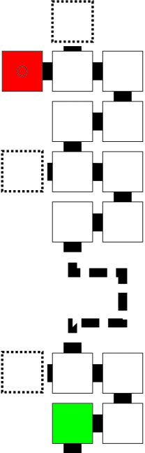
(a) The shaded gadget in the extraction region represents the up-extraction gadget, pictured on the right in Figure 15b. (b) The up-extraction gadget.

Figure 15: Overview of the up-extraction gadget and its location in the overall construction.

The block-number gadget places the correct extraction tile based on the block number position, which is encoded in the geometry of a previous portion of the construction. The placement of an extraction tile either initiates the assembly of the “block-hook” gadget (see Figure 14b) or initiates a different gadget that assembles the perimeter for the final extraction region via a hard-coded path of tiles. First, the block-hook gadget assembles an L-shape path above a portion of the previous extraction region, in the $z=1$ plane, and then builds, in the $z=0$ plane, a geometric pattern of tiles in the shape of a one-tile-wide hook that will later stop the downward growth of the “hook-seeking gadget” (see Figure 20b). Then the block-hook gadget initiates the assembly of the “up-extraction” gadget (see Figure 15b). Finally, the block-hook gadget is responsible for determining the starting point (in the north-south direction) for a subsequent gadget called the “hook-initiating” gadget (see Figure 21b). Note that, as the construction continues, from $k$-bit block to $k$-bit block (except for the first and last blocks, which are hard-coded), the hook of tiles initially assembled by the block-hook gadget is translated up by two tiles (one translation per extraction region). The location of this hook essentially represents which $k$-bit block to extract next.

As mentioned above, the final tile of the block-hook gadget initiates the up-extraction gadget. The up-extraction gadget assembles upward, in a zig-zag pattern (as described above), parallel to the block-number gadget. The top-left tile of each zig-zag pattern tries to grow left but is blocked by a portion of the block-number gadget (this is the zag portion of the path). When the up-extraction gadget grows to the row immediately above the top row of the block-number gadget, the red tile shown in Figure 15b is placed. This tile initiates the “extraction-jump” gadget (see Figure 16b). Subsequently, the upward growth of the up-extraction gadget is blocked by tiles from the previous extraction region. The extraction-jump gadget grows a path of tiles in the $z=1$ plane, above the up-extraction gadget and to the right of a portion of the previous extraction region. In our construction, we have $O(m)$ distinct block-hook gadgets, up-extraction gadgets and extraction-jump gadgets (one for each $k$-bit block). The final tile of the extraction-jump gadget initiates the “extraction” gadget (see Figure 17a).

(a) The shaded gadget in the extraction region represents the extraction-jump extraction gadget, pictured on the right in Figure 16b. (b) The extraction-jump gadget.

Figure 16: Overview of the extraction-jump gadget and its location in the overall construction.

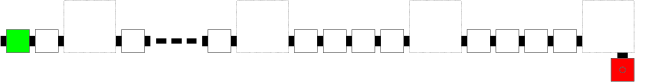
(a) The extraction gadget (see Figure 18 for a detailed view of the large squares in this figure).

(b) The shaded gadget in the extraction region represents the extraction gadget, pictured above in Figure 17a.

Figure 17: Overview of the extraction gadget and its location in the overall construction.

The extraction gadget extracts the current $k$-bit block into a one-bit-per-bump representation along the top of the current extraction region. A bump in the $z=0$ plane is representative of a 0 and a bump in the $z=1$ plane is representative of a 1. These bumps can be seen clearly in Figure 18. Note that the extraction gadget is the result of concatenating $k$ “bit-extraction” gadgets together (see Figure 18). The bit-extraction gadgets are “temperature 1” versions of the “extract bit” (temperature 2) tile types from Figure 5.7a of [12]. The tile complexity of the extraction gadget is $O(m)$ (see our discussion at the end of Section 3.3) and we use the same extraction gadget to extract all $k$-bit blocks.

After the extraction gadget finishes extracting the $k$ bits of the current block, it initiates the assembly of the “ceiling” gadget (see Figure 19a). The ceiling gadget assembles a path of tiles from right to left, placing its final tile under the starting point of the extraction gadget (see the red tile in Figure 19a). Note that, as it assembles toward its ending point, the ceiling gadget places a tile at a carefully chosen location in the $z=1$ plane, the purpose of which is to block a portion of a subsequent gadget, known as the “repeating-up” gadget (see Figure 22b), which we describe later. Due to spacing constraints, this special $z=1$ tile is placed in the column of tiles that is one tile to the left of the penultimate bit-bump of the current extraction region. The placement of this special $z=1$ tile signals a subsequent gadget to assemble the remaining perimeter of the current extraction region and then initiate the assembly of the next extraction region (the gadgets that carry out these tasks will be discussed below). We use a single ceiling gadget in our construction (i.e., the same one is used in all of the $m-2$ generally-constructed extraction regions) and its tile complexity is proportional to the width of an extraction region, which is $O(k)$ and thus $O(m)$. The final tile in the ceiling gadget initiates the assembly of the “hook-seeking” gadget (see Figure 20b).

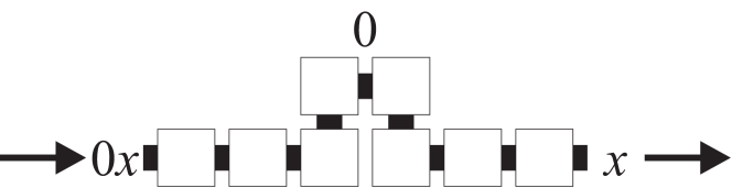
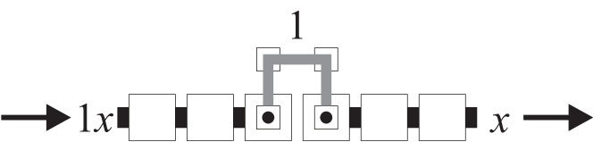
(a) (b)

Figure 18: Magnified view of the bit-extraction gadget to clarify the differences between bumps representing 0s and 1s.

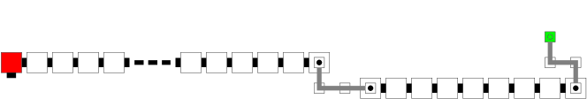
(a) The ceiling gadget.

(b) The shaded gadget in the extraction region represents the ceiling gadget, pictured above in Figure 19a.

Figure 19: Overview of the ceiling gadget and its location in the overall construction.

(a) The shaded gadget in the extraction region represents the hook-seeking gadget, pictured on the right in Figure 20b. (b) The hook-seeking gadget.

Figure 20: Overview of the hook-seeking gadget and its location in the construction.

The hook-seeking gadget starts growing from the final tile that was placed by the ceiling gadget and grows down in a zig-zag pattern, parallel to the previous up-extraction gadget. The hook-seeking gadget grows down until it finds the location of the block hook (see Figure 14b). The assembly of the hook-seeking gadget is very similar to the block-number gadget, i.e., the placement of certain tiles is blocked until the block hook is reached, at which point the downward growth of the hook-seeking gadget is blocked and a special tile is allowed to be placed to the left of the hook-seeking gadget (in the space directly above the block-hook gadget). Once placed, this special tile initiates the assembly of the “hook-initiating” gadget (see Figure 21b). The same hook-seeking gadget is used in all generally-constructed extraction regions.

(a) The shaded gadget in the extraction region represents the hook-initiating gadget, pictured on the right in Figure 21b. (b) The hook-initiating gadget.

Figure 21: Overview of the hook-initiating gadget and its location in the construction.

First, the hook-initiating gadget assembles a path of tiles in the $z=1$ plane directly above a portion of the previous hook-seeking gadget. Then, it assembles a group of tiles in the shape of a two-tile-wide hook in the $z=0$ plane. This hook of tiles will block the downward assembly of the subsequent “repeating-down” gadget (see Figure 24b). When the first repeating-down gadget in the current extraction region is blocked by the hook-initiating gadget, the former will “know” the location of the latter and thus will initiate the assembly of a translated version of the hook (translated up by two tiles). The same hook-initiating gadget is used in all generally-constructed extraction regions. The final tile of the hook-initiating gadget initiates the assembly of the “repeating-up” gadget (Figure 22b).

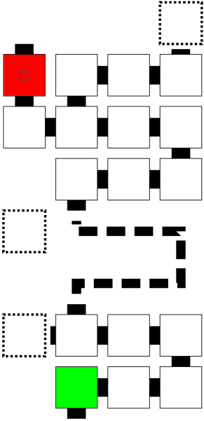
(a) The shaded gadget in the extraction region represents the repeating-up gadget, pictured on the right in Figure 22b. (b) The repeating-up gadget.

Figure 22: Overview of the repeating-up gadget and its location in the construction.

The repeating-up gadget is three tiles wide and uses a zig-zag pattern of assembly to search for the top of the previous repeating-down gadget (or the top of the hook-seeking gadget in the case of the first occurrence of the repeating-up gadget). This top is found when the top-left tile of the zig-zag pattern can place a special tile in one of the locations denoted with a dotted outline (under the red tile) in Figure 22b. Further upward zig-zag growth of the repeating-up gadget is blocked by the ceiling gadget. The tile two tiles south of the big red tile in Figure 22b grows north one location in the $z=0$ plane and is forced to make a decision: either (1) assemble into the $z=1$ plane and initiate the “initiate-repeating-down” gadget (see Figure 23b), or (2) if such growth is blocked in the $z=1$ plane, grow north one more location and initiate the assembly of the “initiate-next-extraction-region” gadget (see Figure 26b). The same repeating-up gadget is used in all generally-constructed extraction regions.

(a) The shaded gadget in the extraction region represents the initiate-repeating-down gadget, pictured on the right in Figure 23b. (b) The initiate-repeating-down gadget.

Figure 23: Overview of the initiate-repeating-down gadget and its location in the construction.

The assembly of the initiate-repeating-down gadget is initiated by the repeating-up gadget. It is basically a line of tiles that assembles in the $z=1$ plane and “jumps” over the top row of the previous repeating-up gadget. An important property of the initiate-repeating-down gadget is that it can only form when a certain tile in the previous repeating-up gadget is not blocked (by a tile in the ceiling gadget) in the $z=1$ plane. The final tile of the initiate-repeating-down gadget initiates the assembly of another repeating-down gadget. The same initiate-repeating-down gadget is used in all generally-constructed extraction regions.

(a) The shaded gadget in the extraction region represents the repeating-down gadget, pictured on the right in Figure 24b. (b) The repeating-down gadget.

Figure 24: Overview of the repeating-down gadget and its location in the construction.

The assembly of a repeating-down gadget is initiated by the final tile of the initiate-repeating-down gadget. The purpose of the repeating-down gadget is to find either the repeating-hook gadget or the hook-initiating gadget (note that the latter scenario only occurs with the first repeating-down gadget within each extraction region). When the hook is found, the repeating-down gadget places a tile at a special location, namely one of the locations denoted by a dotted outline above the red tile in Figure 24b. The red tile placed at this special location initiates the assembly of the “repeating-hook” gadget (see Figure 25b). The same repeating-down gadget is used in all generally-constructed extraction regions.

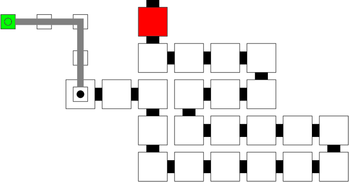
(a) The shaded gadget in the extraction region represents the repeating-hook gadget, pictured on the right in Figure 25b. (b) The repeating-hook gadget.

Figure 25: Overview of the repeating-hook gadget and its location in the construction.

The repeating-hook gadget assembles a path of tiles in the $z=1$ plane in order to avoid a portion of the previous repeating-down gadget. This $z=1$ path assembles right and then down and ultimately assembles a group of tiles in the shape of a hook in the $z=0$ plane, similar to the shape of the hook-initiating gadget. The repeating-hook gadget is initiated by each repeating-down gadget. The main purpose of the repeating-hook gadget is to geometrically propagate the block number position, via the hook of tiles, through the current extraction region. The hook shape of the repeating-hook gadget will also serve to block the downward assembly of the next repeating-down gadget. Note that the final, rightmost hook within an extraction region will serve to block the downward assembly of the block-number gadget of the next extraction region. The same repeating-hook gadget is used in all generally-constructed extraction regions.

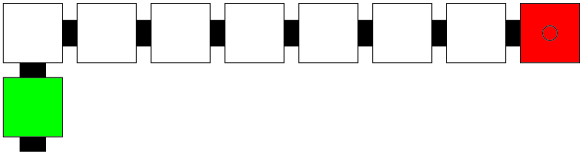
(a) The shaded gadget in the extraction region represents the initiate-next-extraction-region gadget, pictured on the right in Figure 26b. (b) The initiate-next-extraction-region gadget.

Figure 26: Overview of the initiate-next-extraction-region gadget and its location in the construction.

In the case where the repeating-up gadget is blocked in the $z=1$ plane (by a particular tile in the ceiling gadget, as described above), it cannot initiate the assembly of another repeating-down gadget. However, in this case, because of the geometry of the ceiling gadget, the repeating-up gadget may grow a path of tiles in the $z=0$ plane up and underneath part of the ceiling gadget, much like how a highway runs directly underneath an overpass. This is essentially the “signal” from the ceiling gadget to the repeating-up gadget that the current extraction region is almost completed. Note that this signal is hard-coded into the geometry of the ceiling gadget for every extraction region (an obvious consequence of the fact that we use a single ceiling gadget in all generally-constructed extraction regions). The red tile in Figure 22b, in this case, is blocked from growing into the $z=1$ plane, but is unblocked on its north side in the $z=0$ plane and therefore initiates the assembly of the “initiate-next-extraction-region” gadget (see Figure 26b).

(a) The floor gadget.

(b) The shaded gadget in the extraction region represents the floor gadget, pictured above in Figure 27a.

Figure 27: Overview of the floor gadget and its location in the overall construction.

The initiate-next-extraction-region gadget is a short horizontal path of tiles in the $z=0$ plane, the last of which initiates the assembly of the “floor” gadget (see Figure 27a). The same initiate-next-extraction-region gadget is used in all generally-constructed extraction regions.

The assembly of the floor gadget is initiated by the last tile placed by the initiate-next-extraction-region gadget. The floor gadget serves two purposes: it first places tiles along the bottom row of the current extraction region and then it initiates the assembly of the next extraction region by initiating the block-number gadget for the next extraction region. See Figure 27a for an example of how the floor gadget assembles. Since this gadget must assemble a path of tiles of length $O(\textmd{perimeter of an extraction region})$, its tile complexity is $O(m)$. We use the same floor gadget in all generally-constructed extraction regions.

6.2 Construction of a zig-zag counter

In this section, we describe the construction for the binary, $n$-bit, zig-zag counter that we use in our square construction. An example assembly with $n=3$ is depicted in Figure 28. The initial value of the counter is encoded as a geometric pattern of bit-bumps. This seed row, which is part of another construction (in our case, an optimal encoding region or OER), appears as bit-bumps sticking out on the north side of the row of gray tiles at the bottom of Figure 28. In our example, the initial value of the counter is 000. The assembly of the counter starts at the single north glue drawn in orange and sticking out of the OER in the bottom-right corner of the figure. The assembly proceeds by alternating increment rows, assembling from right to left (in blue in the figure) and copy rows, assembling from left to right (in green in the figure). The counter stops when the maximum $n$-bit value is reached, at which point it assembles one additional increment row (in blue) and one flat roof (i.e., with no bumps on the north side), shown as white tiles in the figure. The tile complexity of this construction, which is described in detail in the rest of this section, is $O(1)$.

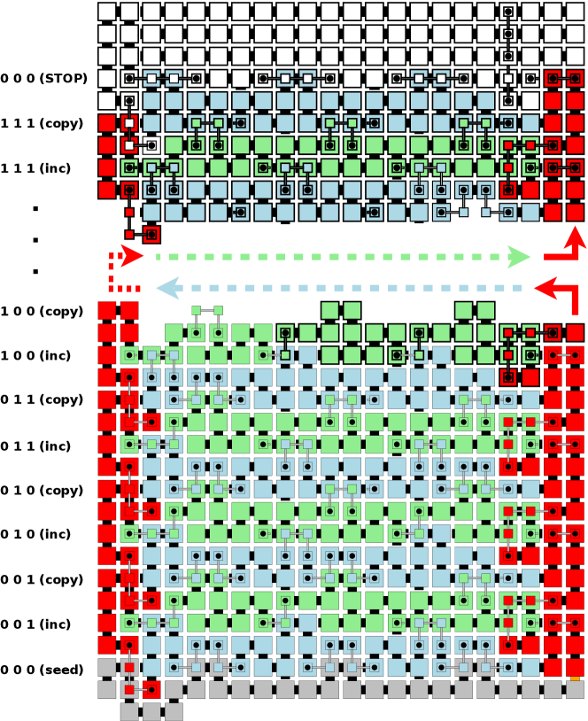
Figure 28: Counter construction. The gray tiles at the bottom of the counter are part of the optimal extraction region that produces the seed value. All other tiles are part of the gadgets shown in Figures 29 and 30. The assembly of the counter starts at the orange glue in the bottom-right corner of the figure.

The counter construction begins with a right wall, that is, the gadget depicted in Figure 29b, that will serve to block the growth of the next copy row. But first, the right-wall gadget initiates an increment row.

The three gadgets needed for the increment rows are shown at the bottom of Figure 29. The main gadget in this group, depicted in Figure 29(e), increments each bit (from 0 to 1 or from 1 to 0). Note that the bit advertised by the previous row is not only incremented but also shifted by two tiles to the left. The second gadget in this group is the copy gadget depicted in Figure 29(d). This gadget is used to leave the bits unchanged in the increment row once the rightmost 0-bit has been incremented and no carry needs to be propagated. Again, the copied bits are shifted by two tiles to the left. This shift also happens with the third gadget in this group, depicted in Figure 29(f), which is specific to the least significant bit of the counter: the notch (i.e., the two missing tiles in the top-right corner of the gadget) will serve as the starting point for a later gadget.

The left-wall gadget, depicted in Figure 29a, is initiated only when the bottom-left tile in any one of the increment gadgets is allowed to grow south. This wall is used to mark the end of the current increment row and initiate the next copy row.

The two gadgets needed for the copy rows are shown at the top of Figure 30. Both gadgets in this group copy each bit (unchanged) and shift the corresponding bit-bump two tiles to the right to compensate for the leftward shift performed in the previous increment row. Each copy row starts with the gadget in Figure 30a that copies the most significant bit of the counter. The other gadget in this group, depicted in Figure 30b, copies all other bits. This gadget also detects the end of the copy row when its bottom-right tile is allowed to grow south (and is simultaneously blocked in its rightward movement in the $z=1$ plane by the right wall that was assembled at the beginning of the previous increment row). At that point, the right-wall foundation gadget (see Figure 29(c)) takes over and initiates another iteration of the increment row/copy row construction by building a right wall.

The next group of gadgets in our construction are used to detect that the maximum value has been reached, that is, when all $n$ bits are equal to 1. These gadgets are modified copies of all of the gadgets that we have described so far. The only difference between each copy and the original gadget is that the new gadget remembers that the most significant bit of the counter has already been incremented to the value 1. These gadgets are not depicted individually since they are identical to the red, blue and green gadgets except for, say, a prime being added to their glue labels. These gadgets, shown with bold outlines in Figure 28, are used exclusively in the “top-half” of the counter construction, or as soon as the “msb right copy” gadget has incremented the most significant bit from 0 to 1 (see the row labelled “1 0 0 (inc)” in Figure 28).

To complete the construction of the counter as a perfect rectangle, we need to build a flat roof on top. This roof construction starts at the south glue of the bottom-left tile in the “copied and modified” (bold) increment gadget. This glue initiates the assembly of the “msb eave” gadget (see Figure 30(c)), which makes up the topmost left wall and allows the roof to assemble. First, the “middle bottom roof” gadget (see Figure 30(d)) is repeated from left to right to form a single row of (white) tiles with no bit-bumps on its north side. Second, the main roof gadget (see Figure 30(e)) is hard-coded to assemble between 1 and 4 rows of tiles (again, with a flat top). The height of this last gadget depends on the target height $h$ of the counter in the following way: the bottommost row in the main roof gadget rounds up the total height of the counter to a multiple of 4 (note that the “middle bottom roof” row and the bottom row of the main roof gadget together play the role of the last green, copy row). Then the number of additional rows in the main roof gadget must be equal to $h$ modulo 4. Therefore, the number of full rows of white tiles in the main roof gadget must be equal to $1+h\bmod{4}$. Of course, the height of the “msb eave” gadget must also be adjusted to match the height of the main roof gadget.

In conclusion, this construction uses an $n$-bit counter to build a rectangle with width $6n+4$ and height $4(2^{n}-i)+r$, where $i$ is the initial value of the counter and $r$ is equal to the height of the counter modulo 4.

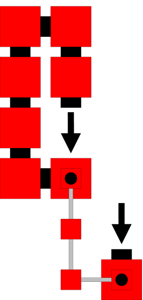
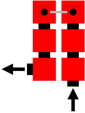
(a) Left-wall gadget (b) Right-wall gadget (c) Right-wall foundation gadget

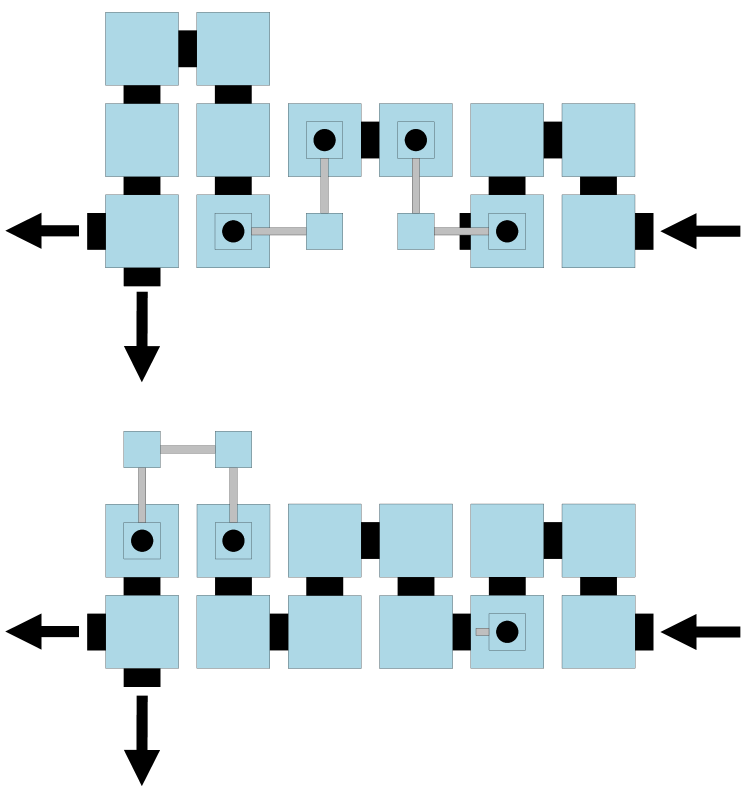
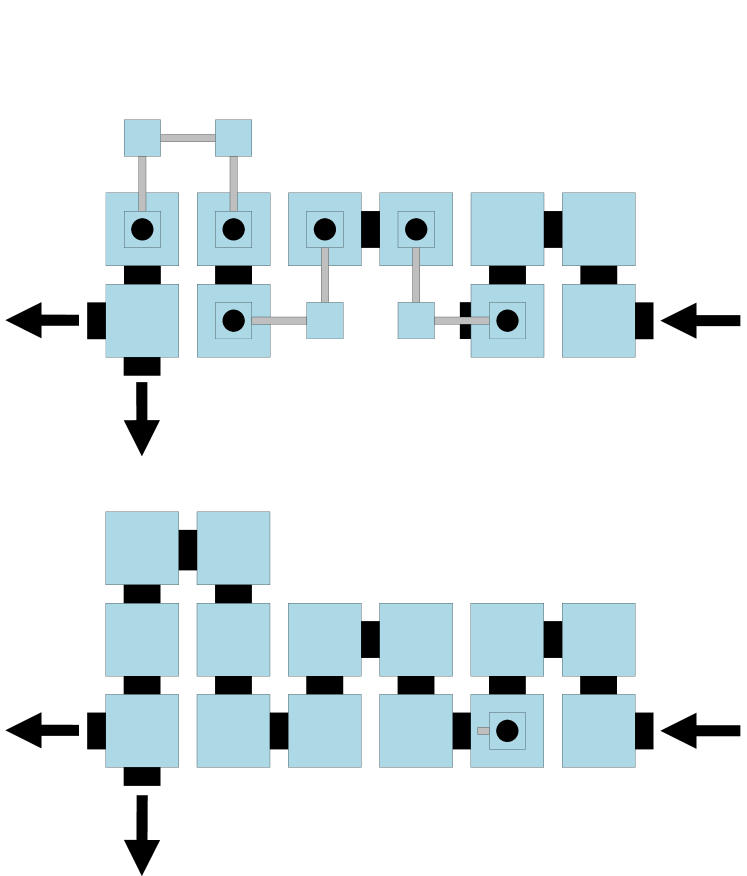
(d) Left copy gadget (top: configuration for bit 0; bottom: configuration for bit 1) (e) Increment gadget (top: incrementing the 0 bit; bottom: incrementing the 1 bit) (f) Lsb increment gadget (top: incrementing the 0 bit; bottom: incrementing the 1 bit)

Figure 29: First set of gadgets used in the construction of the zig-zag counter. In each gadget, the black arrows indicate the entry and exit points of the gadget.

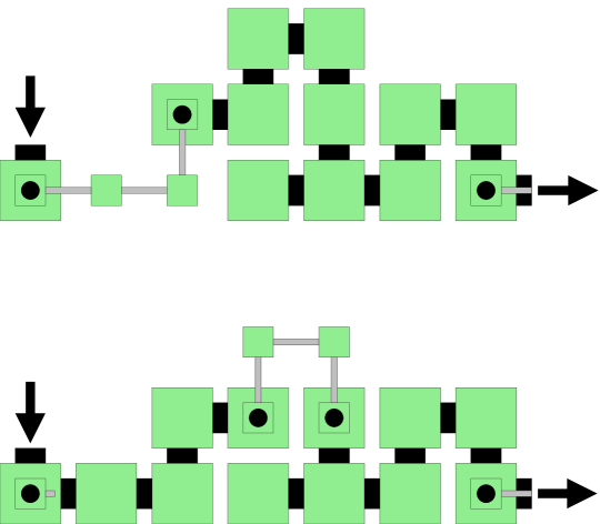
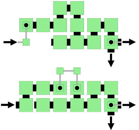
(a) Msb right copy gadget (top: configuration for bit 0; bottom: configuration for bit 1) (b) Right copy gadget (top: configuration for bit 0; bottom: configuration for bit 1)

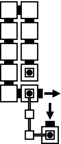
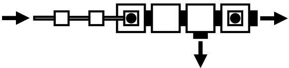
(c) Msb eave gadget: the two-tile-wide leftmost column can vary in height from 2 to 5 tiles (5 tiles are shown above) (d) Middle bottom roof gadget

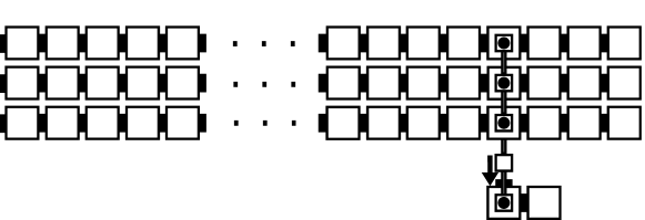
(e) Main roof gadget: The roof itself can vary in height from 1 to 4 tiles (3 are shown here)

Figure 30: Second set of gadgets used in the construction of the zig-zag counter. In each gadget, the black arrows indicate the entry and exit points of the gadget.

References

- [1] Leonard M. Adleman, Qi Cheng, Ashish Goel, and Ming-Deh A. Huang, Running time and program size for self-assembled squares, STOC, 2001, pp. 740–748.
- [2] Sarah Cannon, Erik D. Demaine, Martin L. Demaine, Sarah Eisenstat, Matthew J. Patitz, Robert Schweller, Scott M. Summers, and Andrew Winslow, Two hands are better than one (up to constant factors), Proceedings of the Thirtieth International Symposium on Theoretical Aspects of Computer Science, 2013, pp. 172–184.
- [3] Ho-Lin Chen and David Doty, Parallelism and time in hierarchical self-assembly, SODA 2012: Proceedings of the 23rd Annual ACM-SIAM Symposium on Discrete Algorithms, SIAM, 2012, pp. 1163–1182.
- [4] Qi Cheng, Gagan Aggarwal, Michael H. Goldwasser, Ming-Yang Kao, Robert T. Schweller, and Pablo Moisset de Espanés, Complexities for generalized models of self-assembly, SIAM Journal on Computing 34 (2005), 1493–1515.
- [5] Matthew Cook, Yunhui Fu, and Robert T. Schweller, Temperature 1 self-assembly: Deterministic assembly in 3D and probabilistic assembly in 2D, SODA 2011: Proceedings of the 22nd Annual ACM-SIAM Symposium on Discrete Algorithms, SIAM, 2011.
- [6] David Doty, Matthew J. Patitz, and Scott M. Summers, Limitations of self-assembly at temperature 1, Theoretical Computer Science 412 (2011), 145–158.
- [7] M. Li and P. Vitányi, An introduction to Kolmogorov complexity and its applications (Third Edition), Springer Verlag, New York, 2008.
- [8] Chris Luhrs, Polyomino-safe DNA self-assembly via block replacement, DNA14 (Ashish Goel, Friedrich C. Simmel, and Petr Sosík, eds.), Lecture Notes in Computer Science, vol. 5347, Springer, 2008, pp. 112–126.
- [9] Ján Manuch, Ladislav Stacho, and Christine Stoll, Two lower bounds for self-assemblies at temperature 1, Journal of Computational Biology 17 (2010), no. 6, 841–852.
- [10] Mojżesz Presburger, Über die vollständigkeit eines gewissen systems der arithmetik ganzer zahlen, welchem die addition als einzige operation hervortritt, Compte-rendus du premier Congrès des Mathématiciens des pays Slaves, Warsaw, 1930, pp. 92–101.
- [11] Paul W. K. Rothemund and Erik Winfree, The program-size complexity of self-assembled squares (extended abstract), STOC ’00: Proceedings of the thirty-second annual ACM Symposium on Theory of Computing, 2000, pp. 459–468.
- [12] David Soloveichik and Erik Winfree, Complexity of self-assembled shapes, SIAM J. Comput. 36 (2007), no. 6, 1544–1569.
- [13] Hao Wang, Proving theorems by pattern recognition – II, The Bell System Technical Journal XL (1961), no. 1, 1–41.
- [14] Erik Winfree, Algorithmic self-assembly of DNA, Ph.D. thesis, California Institute of Technology, June 1998.