On linear relaxations of OPF problems
Daniel Bienstock and Gonzalo MuΓ±oz, Columbia University

1 Introduction

. The AC OPF problem is a fundamental software component in the operation of electrical power transmission systems. For background, see [1]. It can be formulated as a nonconvex, continuous optimization problem. In routine problem instances, solutions of excellent quality can be quickly obtained using a variety of methodologies, including sequential linearization and interior point methods. Instances involving grids under stress or extreme conditions can prove significantly more difficult.

The recent work by Lavaei and Low [6] on semidefinite programming relaxations has sparked renewed interest in this problem. See [8] (and references therein) for some cutting-edge approaches.

1.1 Our approach

Here we focus on developing linear relaxations to AC OPF problems, in lifted spaces, with the primary goal of quickly proving lower bounds and enabling fast, standard optimization methodologies such as branching and the incorporation of binary variables into optimization models. To motivate our approach, let $(P,Q,V^{(2)})$ be a vector that includes, for each line $km$, the real and reactive power injections $P_{km},P_{mk},Q_{km}$ and $Q_{mk}$, and for each bus $k$ the squared bus voltage magnitude $|V_{k}|^{2}$, denoted by $V^{(2)}_{k}$. Using these variables, we first write the OPF problem in the following summarized form

$\displaystyle\min$ $\displaystyle F(P,Q,V^{(2)})$ (1a)
Subject to: (1d)
$\displaystyle AP\,+\,BQ\,+\,CV^{(2)}\ \leq\ d$
$\displaystyle(P,Q,V^{(2)})\ \in\ \Omega.$

Here,

  • β€’

    In constraints (1d), $A$, $B$ and $C$ are matrices and $d$ is a vector, all of appropriate dimension. These constraints describe basic relationships such as generator output limits, $(P,Q)$-bus demand statements, and voltage limits. These are all linear constraints and thus can be expressed in the form (1d).

  • β€’

    Constraints (1d) describe the underlying physics, e.g. Ohm’s law. For example, in the rectangular formulation of AC OPF such constraints of course will involve additional variables (the real and imaginary voltage components at each bus) and bilinear constraints relating those variables to the vector $(P,Q,V^{(s)})$.

  • β€’

    In standard OPF problem formulations, the objective $F(P,Q,V^{(2)})$ is typically the sum of active power generation costs (summed over the generators) a separable convex quadratic function of the generator outputs.

Our basic approach will approximate (1d) with linear inequalities obtained by lifting formulation (1) to a higher-dimensional space, and running a cutting-plane algorithm over that lifted formulation. By ’lifting’ we mean a procedure that adds new variables (with specific interpretations) and then writes inequalities that such variables, together with $(P,Q,V^{(s)})$, must satisfy in a feasible solution to the OPF problem. To fix our language, we view the quantities $P_{km},P_{mk},Q_{km},Q_{mk}$ (for each line $km$) and $|V_{k}|^{2}$ (for each bus $k$) as foundational. All other variables, including those that arise naturally from constraint (1d) as well as those that we introduce, will be called lifted111Occasionally we may view the rectangular voltage coordinates as foundational..

In the following sections we introduce our lifted variables, as well as the inequalities that we introduce so as to obtain a convex relaxation of (1d). The inequalities will be of four types:

  1. 1.

    $\Delta$-inequalities,

  2. 2.

    (active power) loss inequalities,

  3. 3.

    Circle inequalities

  4. 4.

    Semidefinite cut inequalities.

All these inequalities are convex; some linear and some conic. In the case of conic inequalities we rely on outer approximation through tangent cutting planes so as to ultimately obtain linear formulations as desired.

In Section 4 we present a tightening procedure, and in Section 5 we describe the use of linear mixed-integer programming.

2 Basic inequalities

We consider a line $\{k,m\}$ with series impedance $z=r+jx$ and series admittance

$\displaystyle y\ \doteq\ z^{-1}=g+jb,\quad\mbox{where}$ (2)
$\displaystyle g=\frac{r}{r^{2}+x^{2}}\quad\mbox{and}\quad b=-\frac{x}{r^{2}+x^{2}}.$ (3)

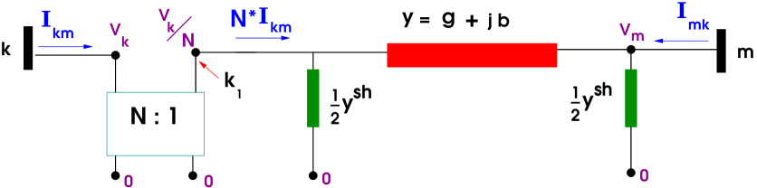
In addition, there will be a shunt admittance ys​h=gs​h+j​bs​hsuperscriptπ‘¦π‘ β„Žsuperscriptπ‘”π‘ β„Žπ‘—superscriptπ‘π‘ β„Žy^{sh}=g^{sh}+jb^{sh}, and a transformer with tap ratio

$\displaystyle N\ \doteq\ \tau e^{j\sigma}$ (4)

where $\tau$ is the magnitude and $\sigma$ is the phase shift angle. Note that $r=r(km)$, etc, but for simplicity of notation we omit the dependence of line parameters on $km$.

Refer to caption
Figure 1: $\pi$-model, including transformer and shunt admittance

In the figure, voltages are shown in purple and currents in blue. Notice that the transformer is assumed to be located at the β€œk” or β€œfrom” end of the line.

Define:

$\displaystyle V$ $\displaystyle=$ $\displaystyle\left(\begin{array}[]{r}V_{k}\\ V_{m}\end{array}\right)=\left(\begin{array}[]{r}|V_{k}|e^{j\theta_{k}}\\ |V_{m}|e^{j\theta_{m}}\\ \end{array}\right)=\left(\begin{array}[]{c}e_{k}+jf_{k}\\ e_{m}+jf_{m}\\ \end{array}\right)\quad\mbox{(voltages at $k$ and $m$)}$ (11)
$\displaystyle I$ $\displaystyle=$ $\displaystyle\left(\begin{array}[]{r}I_{km}\\ I_{mk}\end{array}\right)\quad\quad\mbox{(complex current injections at $k$ and $m$)}$ (14)
$\displaystyle S$ $\displaystyle=$ $\displaystyle\left(\begin{array}[]{r}S_{km}\\ S_{mk}\end{array}\right)\,=\,\left(\begin{array}[]{r}P_{km}+jQ_{km}\\ P_{mk}+jQ_{mk}\end{array}\right)\quad\mbox{(complex power injections at $k$ and $m$)}$ (19)

Then

$\displaystyle S_{km}\ =\ V_{k}I^{*}_{km},\quad S_{mk}\ =\ V_{m}I^{*}_{mk}\quad\mbox{and}\quad I\ =\ \mathbb{Y}V,$ (20)

where $\mathbb{Y}$ is the branch admittance matrix, defined as

$\displaystyle\mathbb{Y}$ $\displaystyle=$ ((y+ys​h2)​1Ο„2βˆ’y​1τ​eβˆ’jβ€‹Οƒβˆ’y​1τ​ej​σy+ys​h2).𝑦superscriptπ‘¦π‘ β„Ž21superscript𝜏2missing-subexpression𝑦1𝜏superscriptπ‘’π‘—πœŽmissing-subexpressionmissing-subexpressionmissing-subexpression𝑦1𝜏superscriptπ‘’π‘—πœŽmissing-subexpression𝑦superscriptπ‘¦π‘ β„Ž2\displaystyle\left(\begin{array}[]{lcr}(y+\frac{y^{sh}}{2})\frac{1}{\tau^{2}}&&-y\frac{1}{\tau e^{-j\sigma}}\\ &\\ -y\frac{1}{\tau e^{j\sigma}}&&y+\frac{y^{sh}}{2}\end{array}\right). (24)

In the next sections we derive the power equations, the $\Delta$ and the circle inequalities, first for the simplest case (no shunt, no transformer) then for the case with shunts but no transformers, and finally for the most general case.

2.1 ys​h=0superscriptπ‘¦π‘ β„Ž0y^{sh}=0 and $N=1$.

In this case we have

$\displaystyle I_{km}$ $\displaystyle=$ $\displaystyle y(V_{k}-V_{m}).$ (25)

In rectangular coordinates this means that

$\displaystyle I_{km}$ $\displaystyle=$ $\displaystyle g(e_{k}-e_{m})-b(f_{k}-f_{m})\,+\,j[\,b(e_{k}-e_{m})+g(f_{k}-f_{m})\,]$ (26)

with a symmetric expression for $I_{mk}$. Therefore

$\displaystyle P_{km}$ $\displaystyle=$ $\displaystyle e_{k}g(e_{k}-e_{m})-e_{k}b(f_{k}-f_{m})+f_{k}g(f_{k}-f_{m})+f_{k}b(e_{k}-e_{m})$ (27)
$\displaystyle=$ $\displaystyle(e_{k}-e_{m})(ge_{k}+bf_{k})+(f_{k}-f_{m})(-be_{k}+gf_{k})$ (28)
$\displaystyle=$ $\displaystyle(e_{k}-e_{m})(g\,,\,b)(^{e_{k}}_{f_{k}})\ +\ (f_{k}-f_{m})(-b\,,\,g)(^{e_{k}}_{f_{k}})$ (29)

with a symmetric expression for $P_{mk}$. Similarly,

$\displaystyle Q_{km}$ $\displaystyle=$ $\displaystyle f_{k}g(e_{k}-e_{m})-f_{k}b(f_{k}-f_{m})-e_{k}g(f_{k}-f_{m})-e_{k}b(e_{k}-e_{m})$ (30)
$\displaystyle=$ $\displaystyle(e_{k}-e_{m})(gf_{k}-be_{k})+(f_{k}-f_{m})(-ge_{k}-bf_{k}).$ (31)

To obtain similar inequalities in polar coordinates we write the impedance and admittance in polar coordinates:

z=|z|​ejβ€‹βˆ β€‹z,y=1|z|​eβˆ’jβ€‹βˆ β€‹z.formulae-sequence𝑧𝑧superscriptπ‘’π‘—βˆ π‘§π‘¦1𝑧superscriptπ‘’π‘—βˆ π‘§z=|z|e^{j\angle z},\quad y=\frac{1}{|z|}e^{-j\angle z}.

Then (see e.g. Bergen and Vittal [1], p. 104)

$\displaystyle S_{km}$ $\displaystyle=$ Vk​Ik​mβˆ—=Vk​(Vkβˆ—βˆ’Vmβˆ—)​yβˆ—=|Vk|2|z|​ejβ€‹βˆ β€‹zβˆ’|Vk|​|Vm||z|​ejβ€‹βˆ β€‹z​ej​θk​m,subscriptπ‘‰π‘˜subscriptsuperscriptπΌπ‘˜π‘šsubscriptπ‘‰π‘˜superscriptsubscriptπ‘‰π‘˜superscriptsubscriptπ‘‰π‘šsuperscript𝑦superscriptsubscriptπ‘‰π‘˜2𝑧superscriptπ‘’π‘—βˆ π‘§subscriptπ‘‰π‘˜subscriptπ‘‰π‘šπ‘§superscriptπ‘’π‘—βˆ π‘§superscript𝑒𝑗subscriptπœƒπ‘˜π‘š\displaystyle V_{k}I^{*}_{km}\ =\ V_{k}(V_{k}^{*}-V_{m}^{*})y^{*}\,=\,\frac{|V_{k}|^{2}}{|z|}e^{j\angle z}-\frac{|V_{k}||V_{m}|}{|z|}e^{j\angle z}e^{j\theta_{km}}, (32)

where

$$\theta_{km}\doteq\theta_{k}-\theta_{m}.$$

We also can rewrite (32) as

$\displaystyle S_{km}$ $\displaystyle=$ $\displaystyle|V_{k}|^{2}(g-jb)-|V_{k}||V_{m}|(g-jb)(\cos\theta_{km}+j\sin\theta_{km})$ (33)
$\displaystyle=$ $\displaystyle|V_{k}|^{2}g-|V_{k}||V_{m}|g\cos\theta_{km}-|V_{k}||V_{m}|b\sin\theta_{km}$
$\displaystyle+j\left[-|V_{k}|^{2}b+|V_{k}||V_{m}|b\cos\theta_{km}-|V_{k}||V_{m}|b\sin\theta_{km}\right].$

Likewise, the power received at $m$ (rather than injected), $-S_{mk}$, satisfies

$\displaystyle-S_{mk}$ $\displaystyle=$ βˆ’|Vm|2|z|​ejβ€‹βˆ β€‹z+|Vk|​|Vm||z|​ejβ€‹βˆ β€‹z​eβˆ’j​θk​m.superscriptsubscriptπ‘‰π‘š2𝑧superscriptπ‘’π‘—βˆ π‘§subscriptπ‘‰π‘˜subscriptπ‘‰π‘šπ‘§superscriptπ‘’π‘—βˆ π‘§superscript𝑒𝑗subscriptπœƒπ‘˜π‘š\displaystyle-\frac{|V_{m}|^{2}}{|z|}e^{j\angle z}+\frac{|V_{k}||V_{m}|}{|z|}e^{j\angle z}e^{-j\theta_{km}}. (34)

We also obtain an expression for $S_{km}$ similar to (33) by switching the $k$ and $m$ symbols.

2.1.1 $\Delta$ and loss inequalities, 1

Let $\mu_{km}$ and $\nu_{km}$ denote known upper bounds on

$$|(g\,,\,b)(^{e_{k}}_{f_{k}})|\quad\mbox{and}\quad|(-b\,,\,g)(^{e_{k}}_{f_{k}})|,$$

respectively. Then, using (29) we obtain:

$\displaystyle|P_{km}|$ $\displaystyle\leq$ $\displaystyle\mu_{km}|e_{k}-e_{m}|\,+\,\nu_{km}|f_{k}-f_{m}|.$ (35)

This is the basic $\Delta$ inequality. Note that the vectors $(^{g}_{b})$ and $(^{-b}_{g})$ are of equal norm and orthogonal, so further elaborations of the $\Delta$-inequalities are possible.

By adding the expression for $P_{km}$ in (33) and the corresponding expression for $P_{mk}$ we obtain

$\displaystyle P_{km}+P_{mk}$ $\displaystyle=$ $\displaystyle g(|V_{k}|^{2}+|V_{m}|^{2})-2g|V_{k}||V_{m}|\cos\theta_{km}\ =\ g|V_{k}-V_{m}|^{2},$ (36)

which can be relaxed as

$\displaystyle g(e_{k}-e_{m})^{2}+g(f_{k}-f_{m})^{2}\ \leq\ P_{km}+P_{mk},$ (37)

or equivalently,

$\displaystyle g|e_{k}-e_{m}|^{2}+g|f_{k}-f_{m}|^{2}\ \leq\ P_{km}+P_{mk}.$ (38)

We term (37) of (38) the loss inequality. Note that by definition $g\geq 0$ (unless by a modeling artifact we have $r<0$). The point of (38) is that in a lifted formulation with variables representing $|e_{k}-e_{m}|$ and $|f_{k}-f_{m}|$, (38) is convex.

2.1.2 Circle inequalities, 1

We can rewrite ineq. (32) as

$\displaystyle S_{km}$ $\displaystyle=$ $\displaystyle C_{km}-B_{km}e^{j\theta_{km}}\quad\mbox{where}$ (39)
$\displaystyle C_{km}$ $\displaystyle\doteq$ |Vk|2|z|​ejβ€‹βˆ β€‹z​andsuperscriptsubscriptπ‘‰π‘˜2𝑧superscriptπ‘’π‘—βˆ π‘§and\displaystyle\frac{|V_{k}|^{2}}{|z|}e^{j\angle z}\ \mbox{and} (40)
$\displaystyle B_{km}$ $\displaystyle\doteq$ |Vk|​|Vm||z|​ejβ€‹βˆ β€‹z.subscriptπ‘‰π‘˜subscriptπ‘‰π‘šπ‘§superscriptπ‘’π‘—βˆ π‘§\displaystyle\frac{|V_{k}||V_{m}|}{|z|}e^{j\angle z}. (41)

Note that $C_{km}$ and $B_{km}$ are obtained in the complex plane by rotating the real numbers $\frac{|V_{m}|^{2}}{|z|}$ and $\frac{|V_{k}||V_{m}|}{|z|}$ (respectively) by the same angle βˆ β€‹zβˆ π‘§\angle z. As $\theta_{km}$ varies, (32) indicates that $S_{km}$ describes a circle (the β€œsending circle”) with center $C_{km}$ and radius

$$\rho\doteq\frac{|V_{k}||V_{m}|}{|z|}.$$

Likewise, $-S_{mk}$ describes a circle (the β€œreceiving circle”) with center $-\frac{|V_{m}|^{2}}{|z|}$ and radius $\rho$. Refer to Bergen and Vittal for more details. Using either circle we can obtain valid convex inequalities. For example, clearly we have

$\displaystyle[\operatorname{Re}(S_{km}-C_{km})]^{2}\ +\ [\operatorname{Im}(S_{km}-C_{km})]^{2}\ \leq\ \rho^{2},\quad\mbox{or in other words}$ (42)
$\displaystyle\left(P_{km}-\frac{r|V_{k}|^{2}}{r^{2}+x^{2}}\right)^{2}\ +\ \left(Q_{km}-\frac{x|V_{k}|^{2}}{r^{2}+x^{2}}\right)^{2}\ \leq\ \frac{|V_{k}|^{2}|V_{m}|^{2}}{r^{2}+x^{2}}.$ (43)

As discussed in Section 1.1, our formulation has variables used to represent $P_{km},Q_{km},|V_{k}|^{2}$ and $|V_{m}|^{2}$. Using these variables (43) is a conic constraint. Using these variables, from (43) we obtain a convex system by adding two lifted variables $\alpha_{km}$, $\beta_{km}$ and the constraints

$\displaystyle P_{km}-\frac{rV_{k}^{(2)}}{r^{2}+x^{2}}$ $\displaystyle=$ $\displaystyle\alpha_{km}$ (44a)
$\displaystyle Q_{km}-\frac{xV_{k}^{(2)}}{r^{2}+x^{2}}$ $\displaystyle=$ $\displaystyle\beta_{km}$ (44b)
$\displaystyle\alpha_{km}^{2}+\beta_{km}^{2}$ $\displaystyle\leq$ $\displaystyle\frac{V_{k}^{(2)}V_{m}^{(2)}}{r^{2}+x^{2}}.$ (44c)

2.2 General ys​hsuperscriptπ‘¦π‘ β„Žy^{sh} but $N=1$

In this case we have

$\displaystyle I_{km}$ $\displaystyle=$ y​(Vkβˆ’Vm)+12​ys​h​Vk,𝑦subscriptπ‘‰π‘˜subscriptπ‘‰π‘š12superscriptπ‘¦π‘ β„Žsubscriptπ‘‰π‘˜\displaystyle y(V_{k}-V_{m})\,+\,\frac{1}{2}y^{sh}V_{k}, (45)

and so in rectangular coordinates

$\displaystyle I_{km}$ $\displaystyle=$ g​(ekβˆ’em)βˆ’b​(fkβˆ’fm)+12​(gs​h​ekβˆ’bs​h​fk)+𝑔subscriptπ‘’π‘˜subscriptπ‘’π‘šπ‘subscriptπ‘“π‘˜subscriptπ‘“π‘šlimit-from12superscriptπ‘”π‘ β„Žsubscriptπ‘’π‘˜superscriptπ‘π‘ β„Žsubscriptπ‘“π‘˜\displaystyle g(e_{k}-e_{m})-b(f_{k}-f_{m})+\frac{1}{2}(g^{sh}e_{k}-b^{sh}f_{k})\,+\, (46)
j​[b​(ekβˆ’em)+g​(fkβˆ’fm)+12​(bs​h​ek+gs​h​fk)].𝑗delimited-[]𝑏subscriptπ‘’π‘˜subscriptπ‘’π‘šπ‘”subscriptπ‘“π‘˜subscriptπ‘“π‘š12superscriptπ‘π‘ β„Žsubscriptπ‘’π‘˜superscriptπ‘”π‘ β„Žsubscriptπ‘“π‘˜\displaystyle\ j[\,b(e_{k}-e_{m})+g(f_{k}-f_{m})+\frac{1}{2}(b^{sh}e_{k}+g^{sh}f_{k})\,].

We will now obtain

$\displaystyle P_{km}$ $\displaystyle=$ $\displaystyle(e_{k}-e_{m})(g\,,\,b)(^{e_{k}}_{f_{k}})\ +\ (f_{k}-f_{m})(-b\,,\,g)(^{e_{k}}_{f_{k}})\,+\,\frac{g^{sh}}{2}(e_{k}^{2}+f_{k}^{2})$ (47)

and

$\displaystyle Q_{km}$ =(ekβˆ’em)​(g​fkβˆ’b​ek)+(fkβˆ’fm)​(βˆ’g​ekβˆ’b​fk)βˆ’bs​h2​(ek2+fk2).absentsubscriptπ‘’π‘˜subscriptπ‘’π‘šπ‘”subscriptπ‘“π‘˜π‘subscriptπ‘’π‘˜subscriptπ‘“π‘˜subscriptπ‘“π‘šπ‘”subscriptπ‘’π‘˜π‘subscriptπ‘“π‘˜superscriptπ‘π‘ β„Ž2subscriptsuperscript𝑒2π‘˜subscriptsuperscript𝑓2π‘˜\displaystyle=(e_{k}-e_{m})(gf_{k}-be_{k})+(f_{k}-f_{m})(-ge_{k}-bf_{k})-\frac{b^{sh}}{2}(e^{2}_{k}+f^{2}_{k}). (48)

Note that expressions in (47) and (48) are obtained from (29) and (31) by adding the terms gs​h2​(ek2+fk2)superscriptπ‘”π‘ β„Ž2subscriptsuperscript𝑒2π‘˜subscriptsuperscript𝑓2π‘˜\frac{g^{sh}}{2}(e^{2}_{k}+f^{2}_{k}) and βˆ’bs​h2​(ek2+fk2)superscriptπ‘π‘ β„Ž2subscriptsuperscript𝑒2π‘˜subscriptsuperscript𝑓2π‘˜-\frac{b^{sh}}{2}(e^{2}_{k}+f^{2}_{k}), respectively.

To obtain similar expressions under polar coordinates, note that the only the expression (45) for $I_{km}$ differs from (25) only in the term 12​ys​h​Vk12superscriptπ‘¦π‘ β„Žsubscriptπ‘‰π‘˜\frac{1}{2}y^{sh}V_{k}. Thus,

$\displaystyle S_{km}$ $\displaystyle=$ Vk​Ik​mβˆ—=Vk​(Vkβˆ—βˆ’Vmβˆ—)​yβˆ—+12​(gs​hβˆ’j​bs​h)​Vk​Vkβˆ—.subscriptπ‘‰π‘˜subscriptsuperscriptπΌπ‘˜π‘šsubscriptπ‘‰π‘˜superscriptsubscriptπ‘‰π‘˜superscriptsubscriptπ‘‰π‘šsuperscript𝑦12superscriptπ‘”π‘ β„Žπ‘—superscriptπ‘π‘ β„Žsubscriptπ‘‰π‘˜superscriptsubscriptπ‘‰π‘˜\displaystyle V_{k}I^{*}_{km}\ =\ V_{k}(V_{k}^{*}-V_{m}^{*})y^{*}+\frac{1}{2}(g^{sh}-jb^{sh})V_{k}V_{k}^{*}. (49)

2.2.1 $\Delta$ and loss inequalities, 2

Using (47), we obtain

|Pk​m|βˆ’gs​h2​Vk(2)subscriptπ‘ƒπ‘˜π‘šsuperscriptπ‘”π‘ β„Ž2superscriptsubscriptπ‘‰π‘˜2\displaystyle|P_{km}|-\frac{g^{sh}}{2}V_{k}^{(2)} $\displaystyle\leq$ $\displaystyle\mu_{km}|e_{k}-e_{m}|\,+\,\nu_{km}|f_{k}-f_{m}|.$ (50)

This is the second version of the $\Delta$-inequality222A common modeling assumption is that gs​h=0superscriptπ‘”π‘ β„Ž0g^{sh}=0.. Since the right-hand side of (47) is obtained by adding gs​h2​(ek2+fk2)superscriptπ‘”π‘ β„Ž2subscriptsuperscript𝑒2π‘˜subscriptsuperscript𝑓2π‘˜\frac{g^{sh}}{2}(e^{2}_{k}+f^{2}_{k}) to the right-hand side of (29), we have the following analogue of (37):

g​(ekβˆ’em)2+g​(fkβˆ’fm)2≀Pk​m+Pm​kβˆ’gs​h2​(Vk(2)+Vm(2)),𝑔superscriptsubscriptπ‘’π‘˜subscriptπ‘’π‘š2𝑔superscriptsubscriptπ‘“π‘˜subscriptπ‘“π‘š2subscriptπ‘ƒπ‘˜π‘šsubscriptπ‘ƒπ‘šπ‘˜superscriptπ‘”π‘ β„Ž2superscriptsubscriptπ‘‰π‘˜2superscriptsubscriptπ‘‰π‘š2\displaystyle g(e_{k}-e_{m})^{2}+g(f_{k}-f_{m})^{2}\ \leq\ P_{km}+P_{mk}-\frac{g^{sh}}{2}(V_{k}^{(2)}+V_{m}^{(2)}), (51)

the second version of our loss inequality, which again is a conic constraint if we introduce appropriate variables.

2.2.2 Circle inequalities, 2

From (49) we get

$\displaystyle S_{km}$ $\displaystyle=$ |Vk|2​(ejβ€‹βˆ β€‹z|z|+12​(gs​hβˆ’j​bs​h))βˆ’|Vk|​|Vm||z|​ejβ€‹βˆ β€‹z​ej​θk​m,superscriptsubscriptπ‘‰π‘˜2superscriptπ‘’π‘—βˆ π‘§π‘§12superscriptπ‘”π‘ β„Žπ‘—superscriptπ‘π‘ β„Žsubscriptπ‘‰π‘˜subscriptπ‘‰π‘šπ‘§superscriptπ‘’π‘—βˆ π‘§superscript𝑒𝑗subscriptπœƒπ‘˜π‘š\displaystyle|V_{k}|^{2}\left(\frac{e^{j\angle z}}{|z|}+\frac{1}{2}(g^{sh}-jb^{sh})\right)-\frac{|V_{k}||V_{m}|}{|z|}e^{j\angle z}e^{j\theta_{km}}, (52)

which again describes a circle, with center and radius, respectively,

|Vk|2​(ejβ€‹βˆ β€‹z|z|+12​(gs​hβˆ’j​bs​h))and|Vk|​|Vm||z|.superscriptsubscriptπ‘‰π‘˜2superscriptπ‘’π‘—βˆ π‘§π‘§12superscriptπ‘”π‘ β„Žπ‘—superscriptπ‘π‘ β„Žandsubscriptπ‘‰π‘˜subscriptπ‘‰π‘šπ‘§\displaystyle|V_{k}|^{2}\left(\frac{e^{j\angle z}}{|z|}+\frac{1}{2}(g^{sh}-jb^{sh})\right)\quad\mbox{and}\quad\frac{|V_{k}||V_{m}|}{|z|}. (53)

Using (52), (53), and since

Re((|Vk|2(ejβ€‹βˆ β€‹z|z|+12(gs​hβˆ’jbs​h)))\displaystyle\operatorname{Re}\left((|V_{k}|^{2}\left(\frac{e^{j\angle z}}{|z|}+\frac{1}{2}(g^{sh}-jb^{sh})\right)\right) $\displaystyle=$ |Vk|2​(rr2+x2+gs​h2)​andsuperscriptsubscriptπ‘‰π‘˜2π‘Ÿsuperscriptπ‘Ÿ2superscriptπ‘₯2superscriptπ‘”π‘ β„Ž2and\displaystyle|V_{k}|^{2}\left(\frac{r}{r^{2}+x^{2}}+\frac{g^{sh}}{2}\right)\ \mbox{and} (54)
Im((|Vk|2(ejβ€‹βˆ β€‹z|z|++12(gs​hβˆ’jbs​h)))\displaystyle\operatorname{Im}\left((|V_{k}|^{2}\left(\frac{e^{j\angle z}}{|z|}++\frac{1}{2}(g^{sh}-jb^{sh})\right)\right) $\displaystyle=$ |Vk|2​(xr2+x2βˆ’bs​h2),superscriptsubscriptπ‘‰π‘˜2π‘₯superscriptπ‘Ÿ2superscriptπ‘₯2superscriptπ‘π‘ β„Ž2\displaystyle|V_{k}|^{2}\left(\frac{x}{r^{2}+x^{2}}-\frac{b^{sh}}{2}\right), (55)

we obtain the following generalization of (43):

Pk​mβˆ’(rr2+x2+gs​h2)​Vk(2)subscriptπ‘ƒπ‘˜π‘šπ‘Ÿsuperscriptπ‘Ÿ2superscriptπ‘₯2superscriptπ‘”π‘ β„Ž2superscriptsubscriptπ‘‰π‘˜2\displaystyle P_{km}-\left(\frac{r}{r^{2}+x^{2}}+\frac{g^{sh}}{2}\right)V_{k}^{(2)} $\displaystyle=$ $\displaystyle\alpha_{km}$ (56a)
Qk​mβˆ’(xr2+x2βˆ’bs​h2)​Vk(2)subscriptπ‘„π‘˜π‘šπ‘₯superscriptπ‘Ÿ2superscriptπ‘₯2superscriptπ‘π‘ β„Ž2superscriptsubscriptπ‘‰π‘˜2\displaystyle Q_{km}-\left(\frac{x}{r^{2}+x^{2}}-\frac{b^{sh}}{2}\right)V_{k}^{(2)} $\displaystyle=$ $\displaystyle\beta_{km}$ (56b)
$\displaystyle\alpha_{km}^{2}+\beta_{km}^{2}$ $\displaystyle\leq$ $\displaystyle\frac{V_{k}^{(2)}V_{m}^{(2)}}{r^{2}+x^{2}}.$ (56c)

2.3 General bs​hsuperscriptπ‘π‘ β„Žb^{sh} and $N$

In this case we have

$\displaystyle I_{km}$ $\displaystyle=$ 1τ​y​[1τ​Vkβˆ’ej​σ​Vm]+12​τ2​ys​h​Vk1πœπ‘¦delimited-[]1𝜏subscriptπ‘‰π‘˜superscriptπ‘’π‘—πœŽsubscriptπ‘‰π‘š12superscript𝜏2superscriptπ‘¦π‘ β„Žsubscriptπ‘‰π‘˜\displaystyle\frac{1}{\tau}y\left[\frac{1}{\tau}V_{k}-e^{j\sigma}V_{m}\right]\,+\,\frac{1}{2\tau^{2}}y^{sh}V_{k} (57)
$\displaystyle=$ 1τ​y​[1τ​Vkβˆ’(cos⁑σ+j​sin⁑σ)​Vm]+12​τ2​(gs​h+j​bs​h)​Vk.1πœπ‘¦delimited-[]1𝜏subscriptπ‘‰π‘˜πœŽπ‘—πœŽsubscriptπ‘‰π‘š12superscript𝜏2superscriptπ‘”π‘ β„Žπ‘—superscriptπ‘π‘ β„Žsubscriptπ‘‰π‘˜\displaystyle\frac{1}{\tau}y\left[\frac{1}{\tau}V_{k}-(\cos\sigma+j\sin\sigma)V_{m}\right]\,+\,\frac{1}{2\tau^{2}}(g^{sh}+jb^{sh})V_{k}. (58)

In rectangular coordinates this can be further expanded as

$\displaystyle I_{km}\ =$
1τ​(g+j​b)​[1τ​(ek+j​fk)βˆ’(cos⁑σ+j​sin⁑σ)​(em+j​fm)]+12​τ2​(gs​h+j​bs​h)​(ek+j​fk)1πœπ‘”π‘—π‘delimited-[]1𝜏subscriptπ‘’π‘˜π‘—subscriptπ‘“π‘˜πœŽπ‘—πœŽsubscriptπ‘’π‘šπ‘—subscriptπ‘“π‘š12superscript𝜏2superscriptπ‘”π‘ β„Žπ‘—superscriptπ‘π‘ β„Žsubscriptπ‘’π‘˜π‘—subscriptπ‘“π‘˜\displaystyle\frac{1}{\tau}(g+jb)\left[\frac{1}{\tau}(e_{k}+jf_{k})-(\cos\sigma+j\sin\sigma)(e_{m}+jf_{m})\right]+\frac{1}{2\tau^{2}}(g^{sh}+jb^{sh})(e_{k}+jf_{k})
$\displaystyle=\frac{1}{\tau}(g+jb)\left[\frac{1}{\tau}(e_{k}+jf_{k})-e_{m}\cos\sigma+f_{m}\sin\sigma-j(e_{m}\sin\sigma+f_{m}\cos\sigma)\right]$
+12​τ2​[gs​h​ekβˆ’bs​h​fk+j​(bs​h​ek+gs​h​fk)]12superscript𝜏2delimited-[]superscriptπ‘”π‘ β„Žsubscriptπ‘’π‘˜superscriptπ‘π‘ β„Žsubscriptπ‘“π‘˜π‘—superscriptπ‘π‘ β„Žsubscriptπ‘’π‘˜superscriptπ‘”π‘ β„Žsubscriptπ‘“π‘˜\displaystyle+\frac{1}{2\tau^{2}}\left[g^{sh}e_{k}-b^{sh}f_{k}+j(b^{sh}e_{k}+g^{sh}f_{k})\right]
$\displaystyle=\frac{1}{\tau}(g+jb)\left[\frac{1}{\tau}e_{k}-e_{m}\cos\sigma+f_{m}\sin\sigma+j(\frac{1}{\tau}f_{k}-e_{m}\sin\sigma-f_{m}\cos\sigma)\right]$
+12​τ2​[gs​h​ekβˆ’bs​h​fk+j​(bs​h​ek+gs​h​fk)].12superscript𝜏2delimited-[]superscriptπ‘”π‘ β„Žsubscriptπ‘’π‘˜superscriptπ‘π‘ β„Žsubscriptπ‘“π‘˜π‘—superscriptπ‘π‘ β„Žsubscriptπ‘’π‘˜superscriptπ‘”π‘ β„Žsubscriptπ‘“π‘˜\displaystyle+\frac{1}{2\tau^{2}}\left[g^{sh}e_{k}-b^{sh}f_{k}+j(b^{sh}e_{k}+g^{sh}f_{k})\right]. (59)

From this expression we obtain:

$\displaystyle\operatorname{Re}I_{km}$ $\displaystyle=$ $\displaystyle\frac{g}{\tau}\left[\frac{e_{k}}{\tau}-e_{m}\cos\sigma+f_{m}\sin\sigma\right]$ (60)
$\displaystyle-\frac{b}{\tau}\left[\frac{1}{\tau}f_{k}-e_{m}\sin\sigma-f_{m}\cos\sigma\right]$
+12​τ2​[gs​h​ekβˆ’bs​h​fk],and12superscript𝜏2delimited-[]superscriptπ‘”π‘ β„Žsubscriptπ‘’π‘˜superscriptπ‘π‘ β„Žsubscriptπ‘“π‘˜and\displaystyle+\frac{1}{2\tau^{2}}\left[g^{sh}e_{k}-b^{sh}f_{k}\right],\quad\mbox{and}
$\displaystyle\operatorname{Im}I_{km}$ $\displaystyle=$ $\displaystyle\frac{b}{\tau}\left[\frac{e_{k}}{\tau}-e_{m}\cos\sigma+f_{m}\sin\sigma\right]$ (61)
$\displaystyle+\frac{g}{\tau}\left[\frac{1}{\tau}f_{k}-e_{m}\sin\sigma-f_{m}\cos\sigma\right]$
+12​τ2​[bs​h​ek+gs​h​fk].12superscript𝜏2delimited-[]superscriptπ‘π‘ β„Žsubscriptπ‘’π‘˜superscriptπ‘”π‘ β„Žsubscriptπ‘“π‘˜\displaystyle+\frac{1}{2\tau^{2}}\left[b^{sh}e_{k}+g^{sh}f_{k}\right].

We can see that in the β€œno-transformer” case, i.e. $\tau=1$ and $\sigma=0$, (60) and (61) match the expansion (46) for $I_{km}$, as desired. We then have:

$\displaystyle P_{km}$ $\displaystyle=$ $\displaystyle\operatorname{Re}V_{k}I^{*}_{km}$ (62)
$\displaystyle=$ $\displaystyle e_{k}\left\{\frac{g}{\tau}\left[\frac{e_{k}}{\tau}-e_{m}\cos\sigma+f_{m}\sin\sigma\right]-\frac{b}{\tau}\left[\frac{1}{\tau}f_{k}-e_{m}\sin\sigma-f_{m}\cos\sigma\right]\right\}$
$\displaystyle+f_{k}\left\{\frac{b}{\tau}\left[\frac{e_{k}}{\tau}-e_{m}\cos\sigma+f_{m}\sin\sigma+\right]+\frac{g}{\tau}\left[\frac{1}{\tau}f_{k}-e_{m}\sin\sigma-f_{m}\cos\sigma\right]\right\}$
+gs​h2​τ2​(ek2+fk2).superscriptπ‘”π‘ β„Ž2superscript𝜏2subscriptsuperscript𝑒2π‘˜subscriptsuperscript𝑓2π‘˜\displaystyle+\frac{g^{sh}}{2\tau^{2}}(e^{2}_{k}+f^{2}_{k}).

We can rewrite (62) as:

$\displaystyle P_{km}$ $\displaystyle=$ $\displaystyle\frac{1}{\tau}\left[\frac{e_{k}}{\tau}-e_{m}\cos\sigma\right](g\,,\,b)(^{e_{k}}_{f_{k}})+\frac{1}{\tau}\left[\frac{1}{\tau}f_{k}-f_{m}\cos\sigma\right](-b\,,\,g)(^{e_{k}}_{f_{k}})$ (63)
+gs​h2​τ2​(ek2+fk2)superscriptπ‘”π‘ β„Ž2superscript𝜏2subscriptsuperscript𝑒2π‘˜subscriptsuperscript𝑓2π‘˜\displaystyle+\,\frac{g^{sh}}{2\tau^{2}}(e^{2}_{k}+f^{2}_{k})
$\displaystyle+\,\frac{ge_{k}f_{m}+be_{k}e_{m}+bf_{k}f_{m}-gf_{k}e_{m}}{\tau}\sin\sigma.$

In the no-transformer case this expression evaluates to

$\displaystyle(e_{k}-e_{m})(g\,,\,b)(^{e_{k}}_{f_{k}})+(f_{k}-f_{m})(-b\,,\,g)(^{e_{k}}_{f_{k}})+\frac{g^{sh}}{2}(e^{2}_{k}+f^{2}_{k})$ (64)

which is the same as (47), as desired. Note that in (63) the third term vanishes when there is no transformer, and the second term vanishes when there is no shunt conductance. We can further rewrite (63) as

$\displaystyle P_{km}$ $\displaystyle=$ $\displaystyle\frac{1}{\tau}\left[\frac{e_{k}}{\tau}-e_{m}\cos\sigma+f_{m}\sin\sigma\right](g\,,\,b)(^{e_{k}}_{f_{k}})+\frac{1}{\tau}\left[\frac{1}{\tau}f_{k}-f_{m}\cos\sigma-e_{m}\sin\sigma\right](-b\,,\,g)(^{e_{k}}_{f_{k}})$ (65)
+gs​h2​τ2​(ek2+fk2).superscriptπ‘”π‘ β„Ž2superscript𝜏2subscriptsuperscript𝑒2π‘˜subscriptsuperscript𝑓2π‘˜\displaystyle+\,\frac{g^{sh}}{2\tau^{2}}(e^{2}_{k}+f^{2}_{k}).

Next we will compute an expression for $P_{mk}$. In the transformer case the line is not symmetric and we first need to compute $I_{mk}$. We have:

$\displaystyle I_{mk}$ $\displaystyle=$ βˆ’1τ​ej​σ​y​Vk+(y+ys​h2)​Vm1𝜏superscriptπ‘’π‘—πœŽπ‘¦subscriptπ‘‰π‘˜π‘¦superscriptπ‘¦π‘ β„Ž2subscriptπ‘‰π‘š\displaystyle-\frac{1}{\tau e^{j\sigma}}yV_{k}+\left(y+\frac{y^{sh}}{2}\right)V_{m} (67)
$\displaystyle=$ $\displaystyle-\frac{1}{\tau}(\cos\sigma-j\sin\sigma)(g+jb)(e_{k}+jf_{k})$
+(g+gs​h/2+j​(b+bs​h/2))​(em+j​fm)𝑔superscriptπ‘”π‘ β„Ž2𝑗𝑏superscriptπ‘π‘ β„Ž2subscriptπ‘’π‘šπ‘—subscriptπ‘“π‘š\displaystyle+\left(g+g^{sh}/2+j(b+b^{sh}/2)\right)(e_{m}+jf_{m})
$\displaystyle=$ $\displaystyle-\frac{1}{\tau}(g+jb)\left[e_{k}\cos\sigma+f_{k}\sin\sigma+j(-e_{k}\sin\sigma+f_{k}\cos\sigma)\right]$
+(g+gs​h/2)​emβˆ’(b+bs​h/2)​fm+j​[(b+bs​h/2)​em+(g+gs​h/2)​fm].𝑔superscriptπ‘”π‘ β„Ž2subscriptπ‘’π‘šπ‘superscriptπ‘π‘ β„Ž2subscriptπ‘“π‘šπ‘—delimited-[]𝑏superscriptπ‘π‘ β„Ž2subscriptπ‘’π‘šπ‘”superscriptπ‘”π‘ β„Ž2subscriptπ‘“π‘š\displaystyle+(g+g^{sh}/2)e_{m}-(b+b^{sh}/2)f_{m}+j\left[(b+b^{sh}/2)e_{m}+(g+g^{sh}/2)f_{m}\right].

Therefore

$\displaystyle\operatorname{Re}I_{mk}$ $\displaystyle=$ $\displaystyle-\frac{g}{\tau}\left[e_{k}\cos\sigma+f_{k}\sin\sigma\right]+\frac{b}{\tau}\left[-e_{k}\sin\sigma+f_{k}\cos\sigma\right]$ (68)
+(g+gs​h/2)​emβˆ’(b+bs​h/2)​fm,and𝑔superscriptπ‘”π‘ β„Ž2subscriptπ‘’π‘šπ‘superscriptπ‘π‘ β„Ž2subscriptπ‘“π‘šand\displaystyle+(g+g^{sh}/2)e_{m}-(b+b^{sh}/2)f_{m},\quad\mbox{and}
$\displaystyle\operatorname{Im}I_{mk}$ $\displaystyle=$ $\displaystyle-\frac{g}{\tau}\left[-e_{k}\sin\sigma+f_{k}\cos\sigma\right]-\frac{b}{\tau}\left[e_{k}\cos\sigma+f_{k}\sin\sigma\right]$ (69)
+(b+bs​h/2)​em+(g+gs​h/2)​fm.𝑏superscriptπ‘π‘ β„Ž2subscriptπ‘’π‘šπ‘”superscriptπ‘”π‘ β„Ž2subscriptπ‘“π‘š\displaystyle+(b+b^{sh}/2)e_{m}+(g+g^{sh}/2)f_{m}.

Thus,

$\displaystyle P_{mk}$ $\displaystyle=$ $\displaystyle\operatorname{Re}V_{m}I^{*}_{mk}$ (70)
$\displaystyle=$ $\displaystyle e_{m}\left\{-\frac{g}{\tau}\left[e_{k}\cos\sigma+f_{k}\sin\sigma\right]+\frac{b}{\tau}\left[-e_{k}\sin\sigma+f_{k}\cos\sigma\right]\right\}$
$\displaystyle+f_{m}\left\{-\frac{g}{\tau}\left[-e_{k}\sin\sigma+f_{k}\cos\sigma\right]-\frac{b}{\tau}\left[e_{k}\cos\sigma+f_{k}\sin\sigma\right]\right\}$
+(g+gs​h/2)​(em2+fm2)𝑔superscriptπ‘”π‘ β„Ž2subscriptsuperscript𝑒2π‘šsubscriptsuperscript𝑓2π‘š\displaystyle+(g+g^{sh}/2)(e^{2}_{m}+f^{2}_{m})
$\displaystyle=$ $\displaystyle\left[e_{m}-\frac{1}{\tau}e_{k}\cos\sigma\right](g\,,\,b)(^{e_{m}}_{f_{m}})+\left[f_{m}-\frac{1}{\tau}f_{k}\cos\sigma\right](-b\,,\,g)(^{e_{m}}_{f_{m}})$
+gs​h2​(em2+fm2)superscriptπ‘”π‘ β„Ž2superscriptsubscriptπ‘’π‘š2superscriptsubscriptπ‘“π‘š2\displaystyle+\frac{g^{sh}}{2}(e_{m}^{2}+f_{m}^{2})
$\displaystyle+\frac{-ge_{m}f_{k}-bf_{m}f_{k}-be_{m}e_{k}+gf_{m}e_{k}}{\tau}\sin\sigma$
$\displaystyle=$ $\displaystyle\left[e_{m}-\frac{1}{\tau}e_{k}\cos\sigma-\frac{1}{\tau}f_{k}\sin\sigma\right](g\,,\,b)(^{e_{m}}_{f_{m}})+\left[f_{m}-\frac{1}{\tau}f_{k}\cos\sigma+\frac{1}{\tau}e_{k}\sin\sigma\right](-b\,,\,g)(^{e_{m}}_{f_{m}})$
+gs​h2​(em2+fm2).superscriptπ‘”π‘ β„Ž2superscriptsubscriptπ‘’π‘š2superscriptsubscriptπ‘“π‘š2\displaystyle+\frac{g^{sh}}{2}(e_{m}^{2}+f_{m}^{2}).

We now turn to the representation of $P_{km}$ and $P_{mk}$ using polar coordinates.

$\displaystyle S_{km}$ $\displaystyle=$ Vk​Ik​mβˆ—=Vk​(1Ο„2​Vkβˆ—βˆ’1τ​eβˆ’j​σ​Vmβˆ—)​yβˆ—+12​τ2​(gs​hβˆ’j​bs​h)​Vk​Vkβˆ—subscriptπ‘‰π‘˜subscriptsuperscriptπΌπ‘˜π‘šsubscriptπ‘‰π‘˜1superscript𝜏2superscriptsubscriptπ‘‰π‘˜1𝜏superscriptπ‘’π‘—πœŽsuperscriptsubscriptπ‘‰π‘šsuperscript𝑦12superscript𝜏2superscriptπ‘”π‘ β„Žπ‘—superscriptπ‘π‘ β„Žsubscriptπ‘‰π‘˜superscriptsubscriptπ‘‰π‘˜\displaystyle V_{k}I^{*}_{km}\ =\ V_{k}\left(\frac{1}{\tau^{2}}V_{k}^{*}-\frac{1}{\tau}e^{-j\sigma}V_{m}^{*}\right)y^{*}+\frac{1}{2\tau^{2}}(g^{sh}-jb^{sh})V_{k}V_{k}^{*}
$\displaystyle=$ Vk​(1Ο„2​Vkβˆ—βˆ’1τ​eβˆ’j​σ​Vmβˆ—)​(gβˆ’j​b)+12​τ2​(gs​hβˆ’j​bs​h)​Vk​Vkβˆ—subscriptπ‘‰π‘˜1superscript𝜏2superscriptsubscriptπ‘‰π‘˜1𝜏superscriptπ‘’π‘—πœŽsuperscriptsubscriptπ‘‰π‘šπ‘”π‘—π‘12superscript𝜏2superscriptπ‘”π‘ β„Žπ‘—superscriptπ‘π‘ β„Žsubscriptπ‘‰π‘˜superscriptsubscriptπ‘‰π‘˜\displaystyle\ V_{k}\left(\frac{1}{\tau^{2}}V_{k}^{*}-\frac{1}{\tau}e^{-j\sigma}V_{m}^{*}\right)(g-jb)+\frac{1}{2\tau^{2}}(g^{sh}-jb^{sh})V_{k}V_{k}^{*}
$\displaystyle=$ |Vk|2​gΟ„2βˆ’|Vk|​|Vm|​gτ​cos⁑(ΞΈk​mβˆ’Οƒ)βˆ’|Vk|​|Vm|​bτ​sin⁑(ΞΈk​mβˆ’Οƒ)+gs​h2​τ2​|Vk|2superscriptsubscriptπ‘‰π‘˜2𝑔superscript𝜏2subscriptπ‘‰π‘˜subscriptπ‘‰π‘šπ‘”πœsubscriptπœƒπ‘˜π‘šπœŽsubscriptπ‘‰π‘˜subscriptπ‘‰π‘šπ‘πœsubscriptπœƒπ‘˜π‘šπœŽsuperscriptπ‘”π‘ β„Ž2superscript𝜏2superscriptsubscriptπ‘‰π‘˜2\displaystyle|V_{k}|^{2}\frac{g}{\tau^{2}}-|V_{k}||V_{m}|\frac{g}{\tau}\cos(\theta_{km}-\sigma)-|V_{k}||V_{m}|\frac{b}{\tau}\sin(\theta_{km}-\sigma)+\frac{g^{sh}}{2\tau^{2}}|V_{k}|^{2}
+j​[βˆ’|Vk|2​bΟ„2+|Vk|​|Vm|​bτ​cos⁑(ΞΈk​mβˆ’Οƒ)βˆ’|Vk|​|Vm|​gτ​sin⁑(ΞΈk​mβˆ’Οƒ)βˆ’bs​h2​τ2​|Vk|2].𝑗delimited-[]superscriptsubscriptπ‘‰π‘˜2𝑏superscript𝜏2subscriptπ‘‰π‘˜subscriptπ‘‰π‘šπ‘πœsubscriptπœƒπ‘˜π‘šπœŽsubscriptπ‘‰π‘˜subscriptπ‘‰π‘šπ‘”πœsubscriptπœƒπ‘˜π‘šπœŽsuperscriptπ‘π‘ β„Ž2superscript𝜏2superscriptsubscriptπ‘‰π‘˜2\displaystyle+j\left[-|V_{k}|^{2}\frac{b}{\tau^{2}}+|V_{k}||V_{m}|\frac{b}{\tau}\cos(\theta_{km}-\sigma)-|V_{k}||V_{m}|\frac{g}{\tau}\sin(\theta_{km}-\sigma)-\frac{b^{sh}}{2\tau^{2}}|V_{k}|^{2}\right].

Similarly,

$\displaystyle S_{mk}$ $\displaystyle=$ |Vm|2​gβˆ’|Vk|​|Vm|​gτ​cos⁑(ΞΈm​k+Οƒ)βˆ’|Vk|​|Vm|​bτ​sin⁑(ΞΈm​k+Οƒ)+gs​h2​|Vm|2superscriptsubscriptπ‘‰π‘š2𝑔subscriptπ‘‰π‘˜subscriptπ‘‰π‘šπ‘”πœsubscriptπœƒπ‘šπ‘˜πœŽsubscriptπ‘‰π‘˜subscriptπ‘‰π‘šπ‘πœsubscriptπœƒπ‘šπ‘˜πœŽsuperscriptπ‘”π‘ β„Ž2superscriptsubscriptπ‘‰π‘š2\displaystyle|V_{m}|^{2}{g}-|V_{k}||V_{m}|\frac{g}{\tau}\cos(\theta_{mk}+\sigma)-|V_{k}||V_{m}|\frac{b}{\tau}\sin(\theta_{mk}+\sigma)+\frac{g^{sh}}{2}|V_{m}|^{2}
+j​[βˆ’|Vm|2​b+|Vk|​|Vm|​bτ​cos⁑(ΞΈm​k+Οƒ)βˆ’|Vk|​|Vm|​gτ​sin⁑(ΞΈm​k+Οƒ)βˆ’bs​h2​|Vm|2].𝑗delimited-[]superscriptsubscriptπ‘‰π‘š2𝑏subscriptπ‘‰π‘˜subscriptπ‘‰π‘šπ‘πœsubscriptπœƒπ‘šπ‘˜πœŽsubscriptπ‘‰π‘˜subscriptπ‘‰π‘šπ‘”πœsubscriptπœƒπ‘šπ‘˜πœŽsuperscriptπ‘π‘ β„Ž2superscriptsubscriptπ‘‰π‘š2\displaystyle+j\left[-|V_{m}|^{2}b+|V_{k}||V_{m}|\frac{b}{\tau}\cos(\theta_{mk}+\sigma)-|V_{k}||V_{m}|\frac{g}{\tau}\sin(\theta_{mk}+\sigma)-\frac{b^{sh}}{2}|V_{m}|^{2}\right].

Hence the active power loss equals

$\displaystyle P_{km}+P_{mk}\ =$
(|Vk|2Ο„2+|Vm|2)​gβˆ’2​g​|Vk|τ​|Vm|​cos⁑(ΞΈk​mβˆ’Οƒ)+gs​h2​τ2​|Vk|2+gs​h2​|Vm|2.superscriptsubscriptπ‘‰π‘˜2superscript𝜏2superscriptsubscriptπ‘‰π‘š2𝑔2𝑔subscriptπ‘‰π‘˜πœsubscriptπ‘‰π‘šsubscriptπœƒπ‘˜π‘šπœŽsuperscriptπ‘”π‘ β„Ž2superscript𝜏2superscriptsubscriptπ‘‰π‘˜2superscriptπ‘”π‘ β„Ž2superscriptsubscriptπ‘‰π‘š2\displaystyle\left(\frac{|V_{k}|^{2}}{\tau^{2}}+|V_{m}|^{2}\right)g-2g\frac{|V_{k}|}{\tau}|V_{m}|\cos(\theta_{km}-\sigma)+\frac{g^{sh}}{2\tau^{2}}|V_{k}|^{2}\ +\ \frac{g^{sh}}{2}|V_{m}|^{2}. (72)

There is an alternative derivation of this equation that proves useful. Consider point $k_{1}$ in Figure 1. The power injection into the line, at $k_{1}$, is equal to $P_{km}$ (i.e. it equals $\frac{V_{k}}{N}(N*I_{km})^{*}=V_{k}I_{km}^{*}=P_{km}$. Moreover by construction the voltage magnitude at $k_{1}$ equals $|V_{k}|/\tau$ and the phase angle difference from $k_{1}$ to $m$ equals $\theta_{km}-\sigma$. We can now recover (72) from (36), with the last two terms account for shunts, as when deriving (51).

2.3.1 $\Delta$ and loss inequalities, 3

In the transformer case there will be two $\Delta$-inequalities. The first is obtained by from (65) by taking absolute values:

|Pk​m|βˆ’gs​h2​τ2​|Vk|2≀subscriptπ‘ƒπ‘˜π‘šsuperscriptπ‘”π‘ β„Ž2superscript𝜏2superscriptsubscriptπ‘‰π‘˜2absent\displaystyle|P_{km}|-\frac{g^{sh}}{2\tau^{2}}|V_{k}|^{2}\ \leq\
$\displaystyle\frac{\mu_{km}}{\tau}\left|\frac{e_{k}}{\tau}-e_{m}\cos\sigma+f_{m}\sin\sigma\right|\,+\,\frac{\nu_{km}}{\tau}\left|\frac{1}{\tau}f_{k}-f_{m}\cos\sigma-e_{m}\sin\sigma\right|.$ (73)

Here as before $\mu_{km}$ and $\nu_{km}$ are known upper bounds on $|(g\,,\,b)(^{e_{k}}_{f_{k}})|$ and $|(-b\,,\,g)(^{e_{k}}_{f_{k}})|$, respectively. Similarly, we obtain a second $\Delta$-inequality from (70):

|Pm​k|βˆ’gs​h2​τ2​|Vm|2≀subscriptπ‘ƒπ‘šπ‘˜superscriptπ‘”π‘ β„Ž2superscript𝜏2superscriptsubscriptπ‘‰π‘š2absent\displaystyle|P_{mk}|-\frac{g^{sh}}{2\tau^{2}}|V_{m}|^{2}\ \leq\
$\displaystyle\mu_{mk}\left|e_{m}-\frac{1}{\tau}e_{k}\cos\sigma-\frac{1}{\tau}f_{k}\sin\sigma\right|\,+\,\nu_{mk}\left|f_{m}-\frac{1}{\tau}f_{k}\cos\sigma+\frac{1}{\tau}e_{k}\sin\sigma\right|.$ (74)

Thus in order to represent these inequalities we need to introduce additional lifted variables used to model $\left|\frac{e_{k}}{\tau}-e_{m}\cos\sigma+f_{m}\sin\sigma\right|$, $\left|e_{m}-\frac{1}{\tau}e_{k}\cos\sigma-\frac{1}{\tau}f_{k}\sin\sigma\right|$, $\left|\frac{1}{\tau}f_{k}-f_{m}\cos\sigma+e_{m}\sin\sigma\right|$ and $\left|f_{m}-\frac{1}{\tau}f_{k}\cos\sigma+\frac{1}{\tau}e_{k}\sin\sigma\right|$. In the no-transformer case the first two variables are equal to $|e_{m}-e_{k}|$ and the last two are equal to $|f_{m}-f_{k}|$. Replacing, in (73) and (74), $|V_{k}|^{2}$ and $|V_{m}|^{2}$ with $V_{k}^{(2)}$ and $V_{m}^{(2)}$ respectively, we obtain the most general form of the $\Delta$-inequalities.

To obtain a loss inequality we apply the reasoning following equation (72). Note that the voltage at point $k_{1}$ satisfies

$\displaystyle V_{k_{1}}$ $\displaystyle=$ $\displaystyle\frac{V_{k}}{N}\ =\ \frac{1}{\tau}(e_{k}+jf_{k})(\cos\sigma-j\sin\sigma)\ =$ (75)
$\displaystyle\frac{1}{\tau}(e_{k}\cos\sigma+f_{k}\sin\sigma)\,+\,j\frac{1}{\tau}(f_{k}\cos\sigma-e_{k}\sin\sigma).$

Since all losses are incurred in the section of the line between $k_{1}$ and $m$, applying (51) we obtain:

$\displaystyle g\left(e_{m}-\frac{1}{\tau}\cos\sigma-\frac{1}{\tau}f_{k}\sin\sigma\right)^{2}+g\left(f_{m}-\frac{1}{\tau}f_{k}\cos\sigma+\frac{1}{\tau}e_{k}\sin\sigma\right)^{2}$
≀Pk​m+Pm​kβˆ’gs​h2​(Vk(2)Ο„2+Vm(2)).absentsubscriptπ‘ƒπ‘˜π‘šsubscriptπ‘ƒπ‘šπ‘˜superscriptπ‘”π‘ β„Ž2superscriptsubscriptπ‘‰π‘˜2superscript𝜏2superscriptsubscriptπ‘‰π‘š2\displaystyle\ \leq\ P_{km}+P_{mk}-\frac{g^{sh}}{2}\left(\frac{V_{k}^{(2)}}{\tau^{2}}+V_{m}^{(2)}\right). (76)

In this form we obtain a convex inequality that employs the auxiliary variables introduced in (74). A similar construction yields an inequality using the auxiliary variables in (73).

2.3.2 Circle inequalities, 3

In the transformer case the structure of the circle inequalities differs due to the asymmetry caused by the transformer. First, the system (56) applied at $m$ is unchanged (i.e. system (56) with $k$ and $m$ interchanged). To obtain a system at $k$ we again consider point $k_{1}$ in Figure (1) and we now obtain:

Pk​mβˆ’(rr2+x2+gs​h2)​Vk(2)Ο„2subscriptπ‘ƒπ‘˜π‘šπ‘Ÿsuperscriptπ‘Ÿ2superscriptπ‘₯2superscriptπ‘”π‘ β„Ž2superscriptsubscriptπ‘‰π‘˜2superscript𝜏2\displaystyle P_{km}-\left(\frac{r}{r^{2}+x^{2}}+\frac{g^{sh}}{2}\right)\frac{V_{k}^{(2)}}{\tau^{2}} $\displaystyle=$ $\displaystyle\alpha_{km}$ (77a)
Qk​mβˆ’(xr2+x2βˆ’bs​h2)​Vk(2)Ο„2subscriptπ‘„π‘˜π‘šπ‘₯superscriptπ‘Ÿ2superscriptπ‘₯2superscriptπ‘π‘ β„Ž2superscriptsubscriptπ‘‰π‘˜2superscript𝜏2\displaystyle Q_{km}-\left(\frac{x}{r^{2}+x^{2}}-\frac{b^{sh}}{2}\right)\frac{V_{k}^{(2)}}{\tau^{2}} $\displaystyle=$ $\displaystyle\beta_{km}$ (77b)
$\displaystyle\alpha_{km}^{2}+\beta_{km}^{2}$ $\displaystyle\leq$ $\displaystyle\frac{V_{k}^{(2)}V_{m}^{(2)}}{\tau^{2}(r^{2}+x^{2})}.$ (77c)

3 Inequalities from semidefinite relaxations

Let $w$ be a subvector of the vector with entries $(1,e_{1},e_{2},\ldots,e_{N},f_{1},f_{2},\ldots,f_{N})^{T}$ where $N$ is the number of buses. Then we can insist that $ww^{T}\succeq 0$. This is a semidefinite constraint. As an alternative, by introducing additional lifted variables we can use linear separating inequalities as a substitute for the semidefinite constraint. Each additional lifted variable corresponds to an entry of the matrix $ww^{T}$.

To fix ideas, suppose that $w=(e_{1},e_{3},f_{2})^{T}$. Then we will have lifted variables corresponding $e_{1}^{2},e_{3}^{2},f_{2}^{2},e_{1}e_{3},e_{1}f_{2},e_{3}f_{2}$, which we denote, respectively, by $e_{1}^{s},e_{3}^{s},f_{2}^{s},ee_{1e},ef_{12}$ and $ef_{32}$. Suppose that particular values of these variables are such that the resulting matrix

$\displaystyle\tilde{W}$ $\displaystyle=$ $\displaystyle\left(\begin{array}[]{lcr}\tilde{e}_{1}^{s}&\tilde{e}e_{13}&\tilde{e}f_{12}\\ \tilde{e}e_{13}&\tilde{e}^{s}_{3}&\tilde{e}f_{32}\\ \tilde{e}f_{12}&\tilde{e}f_{32}&\tilde{f}_{2}^{s}\end{array}\right)\ \not\succeq 0.$ (81)

Let $u\in\mathbb{R}^{3}$ be such that $u^{T}\tilde{W}u<0$. [Given $\tilde{W}$ such a vector can be computed in polynomial time, for example by running an adaptation of the Cholesky factorization procedure, or directly by computing an appropriate eigenvector of $\tilde{W}$.] Then the inequality

$\displaystyle u_{1}^{2}\,e_{1}^{s}+2u_{1}u_{2}\,ee_{13}+2u_{1}u_{3}\,ef_{12}+u_{2}^{2}\,e^{s}_{e}+2u_{2}u_{3}\,ef_{32}+u_{3}^{2}\,f_{s}^{s}\ \geq\ 0$ (82)

is valid, and violated by $\tilde{W}$. We term such an inequality a semidefinite cut. In computation, the (perhaps obvious) requirement that $\|u\|=1$ is important, as is the appropriate choice of bus indices used to construct the vector $w$.

4 Tightening inequalities through reference angle fixings

Above we introduced a family of inequalities for each line of the underlying network. Here we will describe a tightening procedure that can render significant improvements.

Recall the discussion in Section 2 regarding foundational and lifted variables. Thus, the lifted variables include e.g. a variable used to represent the quantity $\left|e_{m}-\frac{1}{\tau}e_{k}\cos\sigma-\frac{1}{\tau}f_{k}\sin\sigma\right|$ introduced in equation (74).

We can express these facts in compact form as follows. As in Section 2, let $(P,Q,V^{(2)})$ indicate the vector of all foundational variables. Here, for each bus $k$ variable $V^{(2)}_{k}$ is used to represent the quantity $|V_{k}|^{2}$. If $N$ and $M$ indicate the number of buses and lines, respectively, then $(P,Q,V^{2})\in\mathbb{R}^{2M+N}$. Let $W$ indicate the vector of all lifted variables, say with $H$ components, and let $K\subseteq\mathbb{R}^{2M+N+H}$ indicate the convex set described by all inequalities introduced above. Then we can represent $(P,Q,V^{(2)},W)\in K$ more compactly by stating that

$\displaystyle(P,Q,V^{(2)})\,\in\,\hat{K}\,\doteq\,{\mathop{\rm proj}}_{\mathbb{R}^{2M+N}}K$ (83)

where $\mathop{\rm proj}_{\mathbb{R}^{2M+N}}K$ is the projection of $K$ to the subspace of the first $2M+N$ variables.

We now describe a procedure for tightening (83). As is well known, fixing an arbitrary bus at an arbitrary angle does not change the set of feasible solutions to a standard OPF problem. Thus, let $\hat{k}$ be a particular bus, and let $\hat{\theta}_{\hat{k}}$ be a particular angle; we can therefore without loss of generality fix $\theta_{\hat{k}}=\hat{\theta}_{\hat{k}}$. How can we take advantage of this fact so as to obtain stronger constraints? Trivially, we can of course enforce $f_{\hat{k}}=\tan\hat{\theta}_{\hat{k}}e_{\hat{k}}$.

Moreover, consider for example the $\Delta$-inequality (35) for a line $\hat{k}m$ (for simplicity we assume the line has zero shunt admittance and no transformer). We repeat the constraint here for convenience:

$\displaystyle|P_{\hat{k}m}|$ $\displaystyle\leq$ $\displaystyle\mu_{\hat{k}m}|e_{\hat{k}}-e_{m}|\,+\,\nu_{\hat{k}m}|f_{\hat{k}}-f_{m}|,$ (84)

where $\mu_{\hat{k}m}$ and $\nu_{\hat{k}m}$ are valid upper bounds on

$$|(g\,,\,b)(^{e_{\hat{k}}}_{f_{\hat{k}}})|\quad\mbox{and}\quad|(-b\,,\,g)(^{e_{\hat{k}}}_{f_{\hat{k}}})|,$$

respectively. [As previously both $b$ and $g$ depend on the line but we omit the dependency for simplicity of notation]. Given that we know $\theta_{\hat{k}}=\hat{\theta}_{\hat{k}}$ we can tighten the estimates on $\mu_{\hat{k}m}$ and $\nu_{\hat{k}m}$, thereby obtaining a tighter inequality from (84). We can likewise tighten many of the inequalities introduced above.

More generally, suppose that rather than fixing $\theta_{\hat{k}}$ to a fixed value, we insist that it is contained in a known set $I(\hat{k})$ (in particular an interval), i.e.

$$\theta_{\hat{k}}\,\in\,I^{(\hat{k})}$$

As just argued we can therefore without loss of generality, tighten the valid inequalities we described in previous section. [This tightening is easiest in the case where the set is in fact an interval.] Let $K\left(\hat{k},I^{(\hat{k})}\right)\subseteq\mathbb{R}^{2M+N+H}$ denote the resulting convex body, and let

Π​(k^,I(k^))≐projℝ2​M+NK​(k^,I(k^)).approaches-limitΞ ^π‘˜superscript𝐼^π‘˜subscriptprojsuperscriptℝ2𝑀𝑁𝐾^π‘˜superscript𝐼^π‘˜\Pi\left(\hat{k},I^{(\hat{k})}\right)\,\doteq\,{\mathop{\rm proj}}_{\mathbb{R}^{2M+N}}K\left(\hat{k},I^{(\hat{k})}\right).

As a consequence of the above observations, we now formally have:

Lemma 4.1

Suppose $(\tilde{P},\tilde{Q},\tilde{V}^{(2)})$ is feasible for the OPF problem. Then for any bus $\hat{k}$, and any set $I^{(\hat{k})}$,

(P~,Q~,V~(2))βˆˆΞ β€‹(k^,I(k^)).~𝑃~𝑄superscript~𝑉2Ξ ^π‘˜superscript𝐼^π‘˜\displaystyle(\tilde{P},\tilde{Q},\tilde{V}^{(2)})\ \in\ \Pi\left(\hat{k},I^{(\hat{k})}\right). (85)

Β 

Of course one can simply enforce (86) by explicitly writing down all the lifted variables and all the constraints used to describe the set $K\left(\hat{k},I^{(\hat{k})}\right)$. Alternatively, one can separate from the convex set Π​(k^,I(k^))Ξ ^π‘˜superscript𝐼^π‘˜\Pi\left(\hat{k},I^{(\hat{k})}\right) and use such cuts as cutting planes. From this perspective, the following result is important:

Corollary 4.2

Suppose $(\tilde{P},\tilde{Q},\tilde{V}^{(2)})$ is feasible for the OPF problem. Then for any family of buses $k_{i}$ ($i\in F$) and sets $I^{(k_{i})}$ we have

$\displaystyle(\tilde{P},\tilde{Q},\tilde{V}^{(2)})\ \in\ \bigcap_{i\in F}\Pi\left(k_{i},I^{(k_{i})}\right).$ (86)

Β 

In other words, in particular, we can separate a given vector $(\tilde{P},\tilde{Q},\tilde{V}^{(2)})$ from sets obtained from our original family of valid inequalities by e.g. fixing one arbitrary bus to an arbitrary angle, and tightening.

5 Lower and upper bounds through linear mixed-integer programming techniques

To address a the OPF problem in rectangular coordinates we use a technique that was originally developed by Glover [3], used in [2] and more recently analyzed in [4]. Suppose $u$ and $v$ are real variables. We wish to approximate the product $uv$ with linear inequalities, to arbitrary precision. Such a goal can be achieved by adding a moderate number of binary variables.

To that effect, assume without loss of generality that $0\leq u\leq 1$, $0\leq v\leq 1$. This can be achieved by translating and scaling the original $u$ and $v$, if they are assumed bounded. Let $T\geq 1$ be an integer. Then we can write

$\displaystyle u$ $\displaystyle=$ $\displaystyle\sum_{j=1}^{T}2^{-j}y_{j}\ +\ \delta$ (87)

where each $y_{j}$ takes value zero or one, and $0\leq\delta\leq 2^{-T}$. Consequently, we can approximate

$\displaystyle\sum_{j=1}^{T}2^{-j}y_{j}v\ \leq\ uv\ \leq\sum_{j=1}^{T}2^{-j}y_{j}v\ +\ 2^{-T}v$ (88)

This expression cannot directly be used because of the bilinear terms $y_{j}v$. However, let us set $w_{j}\doteq y_{j}v$. Then we have

$\displaystyle w_{j}$ $\displaystyle\leq$ $\displaystyle\min\{v,y_{j}\}$ (89a)
$\displaystyle w_{j}$ $\displaystyle\geq$ $\displaystyle\max\{v+y_{j}-1,0\}.$ (89b)

If $y_{j}=1$ this system implies $w_{j}=v$ whereas if $y_{j}=0$ the system yields $w_{j}=0$. Hence the system, over binary $y_{j}$ but continuous $w_{j}$ and $v$ this system is a valid relaxation of the bilinear relationship $w_{j}=y_{j}v$. Thus, system (89) together with

$\displaystyle\sum_{j=1}^{T}2^{-j}w_{j}\ \leq\ uv\ \leq\sum_{j=1}^{T}2^{-j}w_{j}\ +\ 2^{-T}v$ (90)
$\displaystyle y_{j}\,\in\,\{0,1\},\quad 1\leq j\leq K$ (91)

yields an approximation to the quantity $uv$. The bounds in (90) can be used appropriately to substitute each instance of the product $uv$ in an optimization problem with a linear expression.

By performing the binary expansion (87) for selected rectangular coordinates $e_{k}$ or $f_{k}$ (suitably translated and rescaled) all bilinearities in the rectangular OPF formulation are removed. The resulting optimization problem can then be run using a standalone mixed-integer solver; in particular with the goals of attaining good upper bounds (albeit modulo the approximation errors of magnitude $2^{-K}$), improving lower bounds and possibly even proving infeasibility (same caveat as before regarding approximation errors).

6 Initial computational experiments

In the experiments reported here, we implemented the $Delta$, loss and circle inequalities in their most general form. To solver conic and linear programs, we used Gurobi v. 5.6.3 [5]. To solve semidefinite programs, we used the system due to Lavaei and coauthors [7], which also includes a procedure for extracting a feasible rank-one solution from the SDP. All runs were performed on a current workstation with ample physical memory. All running times are in seconds unless indicated.

In the table β€œSDP time” is the time taken to solve the SDP relaxation of the OPF problem, β€œSDP gap” is the percentage gap between the value of the SDP relaxation and the upper bound (value of feasible solution) obtained by the SDP system. β€œSOCP time” and β€œLP time”, are, respectively, the time required to solve our conic relaxation and its first-order (outer) relaxation through a cutting-plane algorithm. β€œSOCP gap” and β€œLP gap” are the percentage gaps relative to the SDP upper bound.

SDP time SDP gap SOCP time SOCP gap LP time LP gap
case9 1.04 0.0002 $\%$ 0.05 0.7899 $\%$ 0.04 0.7899 $\%$
case30 3.40 0.0185 $\%$ 0.23 1.3808 $\%$ 0.35 1.3964 $\%$
case57 4.23 0.0000 $\%$ 0.62 0.9954 $\%$ 1.41 0.9954 $\%$
case118 8.73 0.0045 $\%$ 0.98 1.4645 $\%$ 5.12 1.4642 $\%$
case300 20.29 0.0018 $\%$ 4.62 1.0585 $\%$ 49.61 1.0559 $\%$
case2383wp 13 min 0.6836 $\%$ 2 min 3.6134 $\%$ 1.63 5.6489 $\%$
case2746wp 16 min 0.0375 $\%$ 79.10 1.8593 $\%$ 1.88 3.1235 $\%$
Table 1: Initial computational results.

References

  • [1] A.R. Bergen and V.Β Vittal, Power Systems Analysis. Prentice-Hall (1999).
  • [2] D. Bienstock, Histogram models for robust portfolio optimization, J. Computational Finance 11 (2007), 1–64.
  • [3] F. Glover, Improved Linear Integer Programming Formulations of Nonlinear Integer Problems, Mgt. Science 22 (1975), 455 – 460.
  • [4] A. Gupte, S. Ahmed, M.S. Cheon and S. S. Dey, Solving Mixed Integer Bilinear Problems using MIP Formulations, SIAM J. on Optimization 23 (2013), 721-744.
  • [5] GUROBI. Gurobi Optimizer. http://www.gurobi.com/.
  • [6] J.Β Lavaei and S.Β Low, Zero duality gap in optimal power flow problem, IEEE Trans. Power Systems 27 (2012), 92–107,
  • [7] J.Β Lavaei, personal communication.
  • [8] D.K. Molzahn and Ian A. Hiskens, Sparsity-Exploiting Moment-Based Relaxations of the Optimal Power Flow Problem, in review. (2014)

Tue.Nov..4.192606.2014@littleboy