Spatially resolving a starburst galaxy at hard X-ray energies: NuSTAR, Chandra, and VLBA observations of NGC 253

Abstract

Prior to the launch of NuSTAR, it was not feasible to spatially resolve the hard ($E>10$ keV) emission from galaxies beyond the Local Group. The combined NuSTAR dataset, comprised of three $\sim 165$ ks observations, allows spatial characterization of the hard X-ray emission in the galaxy NGC 253 for the first time. As a follow up to our initial study of its nuclear region, we present the first results concerning the full galaxy from simultaneous NuSTAR, Chandra, and VLBA monitoring of the local starburst galaxy NGC 253. Above $\sim 10$ keV, nearly all the emission is concentrated within 100^′′ of the galactic center, produced almost exclusively by three nuclear sources, an off-nuclear ultraluminous X-ray source (ULX), and a pulsar candidate that we identify for the first time in these observations. We detect 21 distinct sources in energy bands up to 25 keV, mostly consisting of intermediate state black hole X-ray binaries. The global X-ray emission of the galaxy – dominated by the off-nuclear ULX and nuclear sources, which are also likely ULXs – falls steeply (photon index $\mathrel{\hbox to0.0pt{\lower 3.0pt\hbox{$\mathchar 536\relax$}\hss}\raise 2.0pt\hbox{$\mathchar 318\relax$}}3$) above 10 keV, consistent with other NuSTAR-observed ULXs, and no significant excess above the background is detected at $E>40$ keV. We report upper limits on diffuse inverse Compton emission for a range of spatial models. For the most extended morphologies considered, these hard X-ray constraints disfavor a dominant inverse Compton component to explain the $\gamma$-ray emission detected with Fermi and H.E.S.S. If NGC 253 is typical of starburst galaxies at higher redshift, their contribution to the $E>10$ keV cosmic X-ray background is $<1$%.

1. Introduction

During reionization, a large fraction of the ionizing radiation in the Universe may not only be generated by active galactic nuclei (AGN), but also by other sources in starburst galaxies (Fragos et al., 2013; Mesinger et al., 2013; Pacucci et al., 2014). Observing these galaxies at high redshift ($z\sim 4$) may soon be possible with the upcoming Chandra Deep Field 7 Ms survey (P.I. Niel Brandt). However, they will be observed primarily at rest-frame energies above $\sim 5$ keV. To interpret the integrated X-ray emission from these high-$z$ galaxies, we rely on understanding their hard band spectra, which requires determining the nature of the constituent sources producing it.

The observational effort to constrain the X-ray spectrum of starburst galaxies has been underway since the launch of the first hard X-ray experiments (Bookbinder et al., 1980). Early attempts included stacking the HEAO 1 and Einstein data of a sample of 51 FIR-selected starburst galaxies (Rephaeli et al., 1995). Such studies revealed a rather hard X-ray spectral slope (photon index $\Gamma<2$); however, statistical constraints at $E>10$ keV were poor, and possible contamination from the instrumental background and/or from confused nearby sources was problematic. The types of X-ray binaries (XRBs) dominating at hard energies within starburst galaxies could drive such a hard slope (Persic & Rephaeli, 2002). Alternatively, the hard X-ray emission may also be due to a diffuse population of cosmic-ray electrons inverse Compton (IC) scattering the intense FIR radiation field within the starburst to X-ray energies. The exact nature of this emission is so far largely unconstrained, which is an important problem to solve considering that star-forming galaxies are the most numerous X-ray emitting extragalactic population in the Universe (e.g., Hornschemeier et al., 2003; Lehmer et al., 2012).

The NuSTAR observatory includes the first focusing X-ray optics that operate in orbit above 10 keV (Harrison et al., 2013), dramatically increasing imaging resolution and sensitivity at hard X-ray energies. For the first time, we are able to distinguish individual binaries and diffuse non-thermal emission in starburst galaxies and characterize each component independently.

NGC 253 is the pilot, deep observation of the NuSTAR starburst survey program, which also includes simultaneous NuSTAR and Chandra observations of Arp 299 (Ptak et al., 2014), M82, M83, NGC 3256, and NGC 3310. It is an ideal first target since it is one of the nearest starburst galaxies (3.94 Mpc; Karachentsev et al., 2003) and subtends an angular extent (major-axis 23.8^′; Pence, 1980) comparable to the field of view (FOV) of NuSTAR ($\approx$$13\mbox{${}^{\prime}$}\times 13\mbox{${}^{\prime}$}$). Over the last few decades, for this reason, NGC 253 has been a prime target for X-ray observatories such as Einstein (e.g., Fabbiano & Trinchieri, 1984), ROSAT (e.g., Read et al., 1997; Dahlem et al., 1998; Vogler & Pietsch, 1999; Pietsch et al., 2000), ASCA (e.g., Ptak et al., 1997), BeppoSAX (e.g., Persic et al., 1998; Cappi et al., 1999), XMM-Newton (e.g., Pietsch et al., 2001; Bauer & Pietsch, 2005; Bauer et al., 2007, 2008), Chandra (e.g., Strickland et al., 2000; Weaver et al., 2002; Müller-Sánchez et al., 2010; Mitsuishi et al., 2011), and Suzaku (Mitsuishi et al., 2011, 2013).

Broadly summarizing, the above studies showed that NGC 253 contains diverse X-ray emitting populations throughout the galaxy. A thin plasma with temperature of $\sim 0.4$ keV extends several arcminutes along the plane of the disk, centered around the nucleus (Bauer et al., 2007; Mitsuishi et al., 2013). The nucleus itself contains a starburst with a star-formation rate of $\approx$5 $M_{\odot}$ yr^-1, roughly 70% of the rate for the entire galaxy. Emanating from the nuclear starburst is a collimated kpc-scale outflow (with an X-ray component of $kT\sim 1$ keV), extending roughly perpendicular to the galactic disk, which is limb-brightened in diffuse X-ray emission (e.g., Strickland et al., 2000). Within $\sim 150$ pc of the galactic center, a complex line structure of Fe-K emission has been resolved into at least three spectral components from Fe I at 6.4 keV, Fe XXV at 6.7 keV, and Fe XXVI at 7.0 keV, potentially due to the combination of an obscured AGN, supernova (SN) remnants, and/or XRBs (Mitsuishi et al., 2013). Point sources in this region include a heavily obscured ($n_{\rm H}\approx$ [6–10] $\times 10^{23}$ cm^-2) AGN candidate and individual XRBs and the collective emission from sources within star-forming clouds.

A few dozen X-ray point sources have been detected across the disk. Of particular note are three bright point sources within a few arcseconds of each other in the galactic center and another luminous source $\approx$30^′′ to their south, which is most likely a black-hole (BH) XRB (Lehmer et al., 2013). Although these sources were not classified as ultraluminous X-ray sources (ULXs) by Liu & Bregman (2005), who found only one ULX at the edge of the optical disk in ROSAT data, they have since been observed at qualifying luminosities ($L_{\rm X}\mathrel{\hbox to0.0pt{\lower 3.0pt\hbox{$\mathchar 536\relax$}\hss}\raise 2.0pt\hbox{$\mathchar 318\relax$}}10^{39}$ ergs s^-1 Pietsch et al., 2001; Kajava & Poutanen, 2009). Two other off-nuclear point sources have also been observed with ULX luminosities in XMM-Newton and/or Chandra observations (Kajava & Poutanen, 2009).

In addition to X-ray emission from compact objects and thermal gas, star-forming galaxies are expected to produce diffuse non-thermal X-rays from relativistic particle populations interacting in the galaxies’ strong FIR radiation fields. Recently, two of the nearest starburst galaxies, NGC 253 and M82, have been detected at GeV energies with Fermi LAT (Abdo et al., 2010) and at TeV energies with H.E.S.S. (Acero et al., 2009) and VERITAS (VERITAS Collaboration et al., 2009), respectively. Some fraction of this emission is hadronic, originating from the decay of neutral pions produced by inelastic collisions of cosmic-ray nuclei with interstellar gas. Most of the remainder is leptonic, involving interactions between cosmic-ray electrons and interstellar gas (bremsstrahlung) and radiation fields (IC). If the ratio of accelerated nuclei to electrons is similar in starbursts and the Milky Way (with nuclei responsible for $\sim 99$% of the total cosmic-ray radiated power; e.g., Strong et al., 2010), it is generally expected that the $\gamma$-ray luminosity of starbursts results mainly from hadronic emission. However, significant leptonic emission is predicted by some models (see, e.g., Domingo-Santamaría & Torres, 2005; Rephaeli et al., 2010; Paglione & Abrahams, 2012; Lacki et al., 2012). This distinction may be important for understanding feedback processes in actively star-forming environments (e.g., Booth et al., 2013; Jubelgas et al., 2008; Salem & Bryan, 2013; Socrates et al., 2008; Uhlig et al., 2012), since the inferred non-thermal energy density in both cosmic rays and magnetic fields is larger in hadronic scenarios. At hard X-ray energies, IC emission is the dominant non-thermal emission process, and its detection can directly break the degeneracy between the hadronic and leptonic scenarios because the relevant radiation fields can be estimated from FIR observations (see, e.g., Lacki et al., 2012; Chakraborty & Fields, 2013). Upper limits on diffuse IC emission imply lower bounds on both the cosmic-ray energy density and the strength of magnetic fields.

While the diffuse emission from non-thermal and thermal gas does not vary over day-to-year timescales, XRB X-ray emission most certainly does. This variability results from transitions between various accretion states onto the compact object, during which a thermal accretion disk and/or non-thermal corona drives the emission (e.g., Remillard & McClintock, 2006). It can also manifest more dramatically in flares, which are often associated with radio emission: e.g., Gregory et al. (1972), who found the first strong flares from Cygnus X-3, and Tananbaum et al. (1972), who found the first connection between the X-ray spectral state and the radio brightness in Cygnus X-1. Most of the well-studied Galactic X-ray transients are low mass XRBs (LMXBs), and their radio luminosities are such that current facilities can only find them in the very nearest galaxies (Middleton et al., 2013).

However, a few Galactic XRBs have been found to be extremely radio-bright. The most radio-luminous is Cygnus X-3, which has flares reaching 20 Jy (e.g., McCollough et al., 2010) and is located at a distance of about 9 kpc (Predehl et al., 2000). It is probably not a coincidence that the donor star in Cyg X-3 is a high mass Wolf-Rayet star – it is likely that the jet in Cyg X-3 is far more radiatively efficient than other jets because much of the kinetic power is dissipated on a small spatial scale through interactions with the stellar wind from the mass donor. No such strong flaring has conclusively been seen in other galaxies, but there has been the detection of an extremely strong radio flare without an X-ray counterpart in M82 (Muxlow et al., 2010; Joseph et al., 2011), which may be the same phenomenon. In classical XRBs, the radio emission is well-correlated with the hard X-rays, and the radio flares seem to take place at the transition from a hard spectral state to a soft one, perhaps due to shocking of the fast moving jet against slower-moving older jet material as the jet speeds up (Vadawale et al., 2003). In Cygnus X-3, the situation is slightly different, with strong radio flares being seen on the return from the soft state to the hard state (Koljonen et al., 2010), rather than at times of spectral softening like in other systems. Given that the very brightest Galactic XRB in the radio shows unusual properties relative to other systems, and is clearly associated with a young mass donor, searching for more such objects in nearby galaxies with higher star formation rates (and thus a higher proportion of high mass XRBs, or HMXBs) may help unravel the causes of these differences.

Two previous studies utilized our nearly simultaneous NuSTAR and Chandra observations of NGC 253 to investigate variable sources. Lehmer et al. (2013) established that the 3–40 keV X-ray emission of the nuclear region is dominated by XRB populations and ULX sources rather than accretion onto a supermassive BH. Maccarone et al. (2014) combined the Chandra data with archival Chandra and XMM-Newton observations to reveal another, non-nuclear source with dramatic variability. Its variability is consistent with a $\approx$15 hour period, making it a strong new candidate for being a rare Wolf-Rayet HMXB.

In this paper, we utilize the NuSTAR and Chandra data to investigate the populations contributing to the galaxy-wide 0.5–30 keV emission from NGC 253. Our key goals are to provide the first-ever hard X-ray spectral constraint on a starburst galaxy by (1) measuring the accretion states of the bright XRB population in a starburst galaxy environment and (2) placing the most sensitive constraints on diffuse IC emission in a nuclear starburst. Our paper is organized as follows. In Section 2 we discuss the reduction of the X-ray and radio datasets and the analysis of the non-NuSTAR observations. In Section 3 we describe the methodology behind the use of calibration products in the NuSTAR data analysis. Section 4 assesses the diffuse and point-like components contributing to the galaxy-wide emission in the combined observation. In Section 5 we investigate the variability of the brightest sources and the results of the radio campaign. Finally, in Section 6 we interpret our results and discuss future studies.

All X-ray fluxes and luminosities quoted here have been corrected for Galactic absorption, assuming the column density in the direction of NGC 253 of $1.4\times 10^{20}$ cm^-2 (Stark et al., 1992). At the distance of NGC 253, 1^′′ subtends a physical distance of 19 pc. Unless stated otherwise, quoted uncertainties correspond to 90% confidence intervals.

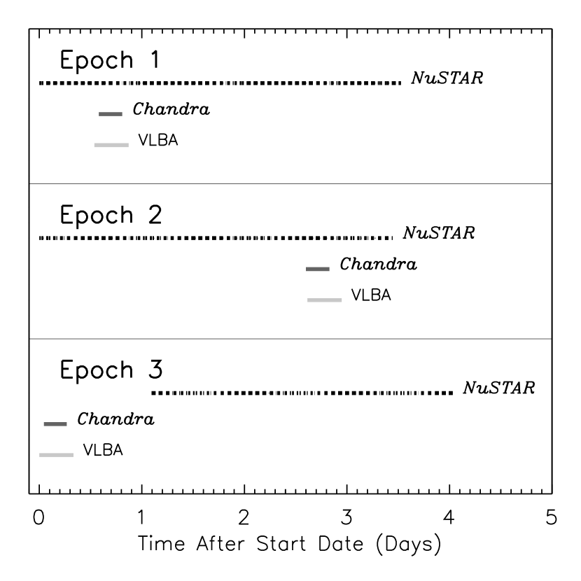
Figure 1.— Relative NuSTAR (black, dashed lines), Chandra (dark gray lines), and VLBA (light gray lines) observational coverage for each of the three epochs. For clarity, we have annotated the total range of observational dates for each epoch. The breaks in the NuSTAR observational window are due primarily to Earth occultations and passages through the South Atlantic Anomaly. Additional details are summarized in Table 2.1.

2. Data and Initial Reduction

Hard X-ray, soft X-ray, and radio observations were carried out with the NuSTAR, Chandra, and VLBA observatories over 3 near simultaneous epochs, illustrated in Figure 1 and summarized with ObsIDs in Table 2.1. The scientific focus of this paper is based on sources detected in the three NuSTAR observations, with the Chandra data primarily providing identifications.

2.1. NuSTAR

Each $\approx$165 ks NuSTAR exposure utilize data from focal plane modules “A” and “B,” which image the same $\approx$$13\mbox{${}^{\prime}$}\times 13\mbox{${}^{\prime}$}$ region centered on the nucleus. The data were reduced using HEASoft v6.14, nustardas v1.2.0, and the associated CALDB release. We began by bringing level 1 data to level 2 products by running nupipeline, which performs a variety of data processing functions, including, e.g., filtering out bad pixels, screening for cosmic rays and observational intervals when the background was too high (e.g., during passes through the South Atlantic Anomaly), and accurately projecting the events to sky coordinates by determining the optical axis position and correcting for mast motions. The task nupipeline was executed with the following flags included: SAAMODE=STRICT and TENTACLE=yes. These additional flags reduce the cleaned exposure time by $\sim 15$% from what it would otherwise be, but also reduce background uncertainties. No strong fluctuations are present in light curves produced from the cleaned events, suggesting a stable background, so no further time periods were excluded. Images culled from the cleaned events are background subtracted – following the description in Section 3.1 – for each epoch and combined in Figure 2.

NuSTAR-only source catalogs are not independently created but based on Chandra positions (Section 2.2) by the methodology described in Section 4.1.1.

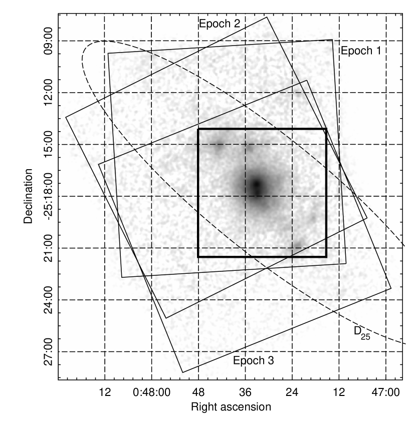
Figure 2.— The combined, background-subtracted 4-25 keV NuSTAR image of NGC 253 from both A and B telescopes and all three epochs: the approximate 13^′$\times$13^′  FOV is indicated in each case. The image has been smoothed with a 3 pixel ($\sim 7.4\mbox{${}^{\prime\prime}$}$) Gaussian kernel and is logarithmically scaled from 0 cts pix^-1 to 40 cts pix^-1. The dashed ellipse marks the optical $D_{25}$ radius of the disk. The exposure time of each epoch is given in Table 2.1. In this work, we focus on the central overlapping region outlined by the thickly drawn box.

Table 1Observation Log

& 2012 Sept 1 50002031002 143.4/143.9 ks
NuSTAR FPMA/B 2012 Sept 15 50002031004 141.7/141.5 ks
2012 Nov 16 50002031006 113.5/113.4 ks
2012 Sept 2 13830 19.7 ks
Chandra ACIS-I 2012 Sept 18 13831 19.7 ks
2012 Nov 16 13832 19.2 ks
2012 Sept 2 SD679A 8 hr
VLBA 2012 Sept 18 SD679B 8 hr
2012 Nov 16 SD679C 8 hr

2.2. Chandra

All three of the $\approx$20 ks Chandra exposures were conducted using single $16.9\mbox{${}^{\prime}$}\times 16.9\mbox{${}^{\prime}$}$ ACIS-I pointings (ObsIDs 13830, 13831, and 13832) with the approximate position of the nucleus set as the aimpoint. For our data reduction, we used CIAO v. 4.4 with CALDB v. 4.5.0. We reprocessed our events lists, bringing level 1 to level 2 using the script chandra_repro, which identifies and removes events from bad pixels and columns, and filters events lists to include only good time intervals without significant flares and non-cosmic ray events corresponding to the standard ASCA grade set (grades 0, 2, 3, 4, 6). We constructed an initial Chandra source catalog by searching a 0.5–7 keV image using wavdetect (run with a point spread function [PSF] map created using mkpsfmap), which was set at a false-positive probability threshold of $2\times 10^{-5}$ and run over seven scales from 1 to 8 (spaced out by factors of $\sqrt{2}$ in wavelet scale: 1, $\sqrt{2}$, 2, 2$\sqrt{2}$, 4, 4$\sqrt{2}$, and 8). Each initial Chandra source catalog was cross-matched to an equivalent catalog, which we created following the above procedure using a moderately deep ($\approx$80 ks) Chandra ACIS-S exposure from 2003 September 20 (ObsID: 3931). The 2003 observation is the deepest Chandra image available for NGC 253 and has an aimpoint close to those of the three 2012 observations. For the purpose of comparing point sources in the 2012 observations with those of the deep 2003 exposure (see Lehmer et al. 2013), we chose to register the 2012 aspect solutions and events lists to the 2003 frame using CIAO tools reproject_aspect and reproject_events, respectively. The resulting astrometric reprojections gave very small astrometric adjustments, including linear translations of $\delta x=-0.49$ to +0.37 pixels and $\delta y=+$0.28 to 0.37 pixels, rotations of $-0.026$ to $-0.004$ deg, and pixel scale stretch factors of 0.999963 to 1.000095. The final pixel scale of all observations was 0.492 arcsec pix^-1.

We constructed Chandra source catalogs for each of the three epochs in the 4–6 keV bandpass, which overlaps with the NuSTAR response. These catalogs were created by searching 4–6 keV images with wavdetect (at a false-positive probability threshold of $10^{-6}$) using a 90% enclosed count fraction PSF map. In Section 4.1.1, we utilize the 4–6 keV Chandra source catalogs and properties as priors when computing the NuSTAR point source photometry.

2.3. VLBA

In order to search for radio emission from X-ray sources distributed across the 14^′ field of NGC 253, we made use of the new wide-field capabilities of the DiFX software correlator (Deller et al., 2011), correlating a large number of sky positions (“phase centers”) in a single correlation pass, thus allowing us to produce radio maps covering each of the Chandra and NuSTAR sources. This strategy is necessary because very long baseline interferometry (VLBI) images made at each phase center are typically limited to only a few arcseconds in diameter. Even though DiFX represents a major gain over standard correlators in terms of studying a wider area of the galaxy, there is still a limit to the number of correlations one can perform. Our strategy was to perform correlations (i.e., search for radio emission) at the locations of NuSTAR and Chandra point sources, which might exhibit rising hard band emission correlated to a radio flare.

We observed NGC 253 at a frequency of 1.4 GHz in three eight-hour sessions, carried out using all ten antennas of the VLBA (see Fig. 1 and Table 2.1). At 1.4 GHz, the resolution of our observations is $\sim 5-10$ milli-arcseconds (with an elliptical beam due to the low declination of the galaxy) and the largest angular scale to which the array is sensitive is $\sim 180$ milli-arcseconds. Following quick ($\mathrel{\hbox to0.0pt{\lower 3.0pt\hbox{$\mathchar 536\relax$}\hss}\raise 2.0pt\hbox{$\mathchar 316\relax$}}24$ hr) processing of the Chandra and NuSTAR images at each epoch, a point-source list was drawn up of positions to use as correlation phase centers, based on the sources detected in the X-ray images. Phase centers were also included in a grid covering the core region where most of the known VLBI-detected components are located. Correlation parameters were chosen to (1) allow imaging of each field out to a radius of $\approx 40\mbox{${}^{\prime\prime}$}$ with a loss of $\approx 10$% in sensitivity at the image edge; (2) allow reliable imaging of fields up to 15^′ from the pointing center of the observation; (3) provide a theoretical 5$\sigma$ sensitivity of 150 $\mu$Jy/beam; and (4) keep the correlator output data rate within practical limits. Following correlation, the $\approx 70$ individual data sets per epoch were transferred to a local machine for processing. Data reduction was carried out using standard methods for phase referencing experiments with the VLBA including: interference rejection, fringe fitting, and phase and amplitude calibration. The first field was calibrated by hand, then a custom software pipeline was used to transfer the calibration solutions to each phase center and image the data sets. Each field was imaged in four overlapping squares, each covering a quarter of the entire $\approx 40\mbox{${}^{\prime\prime}$}$ field. The images were searched for sources with a source finder and inspected by eye. Most phase center positions were correlated in more than one epoch; these matching calibrated datasets were combined in the $u-v$ plane and processed to produce images with a lower noise limit. A more detailed description of the observations and data analysis methods will be presented in Argo et al. (in prep.).

3. Further NuSTAR Data Processing

The NGC 253 X-ray point source population, fairly well characterized at $E<8$ keV by Chandra, is a crowded field for the NuSTAR PSF (see Fig. 3), which has an 18^′′ full width at half maximum (FWHM) core and 58^′′ half power diameter (Harrison et al., 2013). Even for sources outside the nuclear region, the wings of the PSF of bright ULXs in and to the south of the nucleus complicate standard source analysis (see Fig. 2 of Lehmer et al., 2013). Similarly, local annular background regions would be contaminated by redistributed source emission. A gradient in NuSTAR’s $E\lesssim 15$ keV background also prevents spectra extracted from regions far from sources to be simply scaled and subtracted from source regions (e.g., Wik el al., 2014). We describe our approach to the data analysis below.

3.1. Background Modeling

We characterize the background using the tool nuskybgd, which is described in detail in Wik el al. (2014). Briefly, source-free regions are used to determine the components of a background model developed from extragalactic survey observations. Each component has an assumed spectral and spatial structure, so once the overall normalization of each component – which can vary from observation to observation – is found somewhere within the FOV, the model can be extrapolated across the FOV. We extract spectra from four non-source regions in each epoch, simultaneously fit them with the background model, and use those best-fit parameters to create spatial and spectral backgrounds at source locations. These regions cover roughly the entire area within the FOV except for where source emission is present, which largely corresponds to the thickly drawn box in Figure 2. We divide the background into rectangular segments that align with the roll angle of that epoch and range in solid angle from 10–40 arcmin².

In addition to the standard “Aperture” background component, which accounts for stray light (i.e., unreflected photons) from the cosmic X-ray background (CXB) reaching the detectors through the aperture stops, very bright CXB sources 1°–5° from the target can similarly shine directly on the detectors and distort the background shape and spectrum. The Seyfert 2 galaxy NGC 235A is 4.2° away, and its Swift BAT flux (Winter et al., 2009) makes it a marginal candidate for contamination. During the background modeling, we add a component with its hard X-ray spectrum in each region with free normalization. We find that inclusion of the new component does not appreciably affect the resulting background model; the surface brightness of NGC 235A is roughly comparable to that of the CXB focused by the optics, which accounts for at most 10% of the background below 10 keV.

3.2. PSF Modeling

The NuSTAR PSF shape is well calibrated (see Harrison et al., 2013, for details) as a function of off-axis angle, which distorts the PSF into a banana-like shape far ($>3\mbox{${}^{\prime}$}$) from the optical axis. The distortions are similar in relative magnitude to those seen in XMM-Newton, which are not nearly as dramatic as those in Chandra. Additionally, pointing variations cause a given source’s off-axis angle to wander $\lesssim 1$^′  over the course of an observation. While this motion, removed by a metrology system, is unimportant for the PSF of sources $\lesssim 3$^′  from the optical axis, at larger off-axis angles the PSF shape for a source can change non-negligibly during an observation. A few of our sources are this far off-axis, so we create composite PSFs by combining PSF models (stored in the CALDB as images) weighted by the time spent at each off-axis angle.

After attempting to fit these PSFs to sources in our observations, we find that the model PSF core is sharper than what is present in these data. Simply smoothing the PSF image by 2 pixels ($\sim 5$^′′) yields a much more satisfactory fit, especially in the core. This additional smearing of the PSF may result from the accumulation of pointing reconstruction errors (i.e., jitter) over these long exposure times. A jitter of a few arcseconds would be consistent with NuSTAR’s absolute astrometry, so shifts in the astrometric solution over a long observation seem reasonable. The PSFs in the CALDB, having been calibrated from shorter observations of bright sources, may not include this effect. In any case, we find that the smoothed PSFs appear to successfully capture the emission from point sources in these data, which are the deepest NuSTAR observations to clearly image multiple point sources across a $\sim 6\mbox{${}^{\prime}$}$ FOV outside of the Galactic center. Note that these PSFs include no energy dependence, even though the PSF does broaden slightly below $\sim 8$ keV. Energy-dependent PSFs appear in versions of the CALDB after and including v20131007.

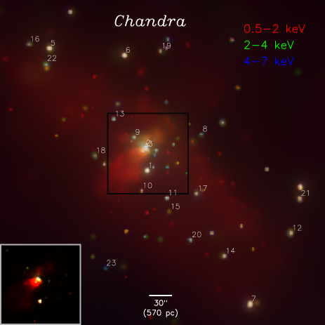
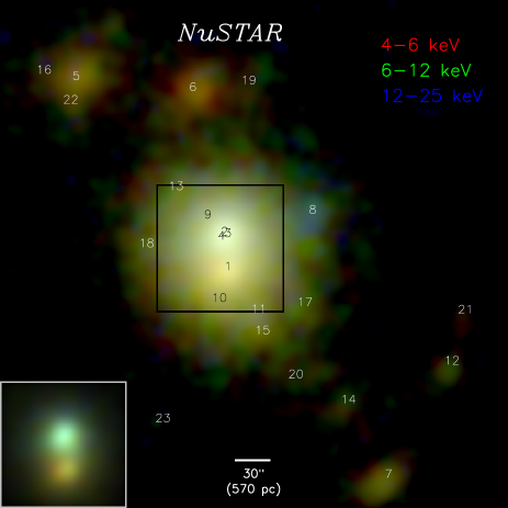
Figure 3.— False color images (logarithmically scaled) of the Chandra (left) and NuSTAR (right) data in the 7.4^′$\times$7.4^′ region centered on the nucleus. Detected NuSTAR sources are numbered as in Table 4.1.1. Source IDs are sorted by their 4–25 keV count rates in descending order. We use the higher spatial resolution of Chandra to de-convolve the NuSTAR data (see Section 3.2 on PSF modeling and Section 4.1.1 on its application), which is particularly important in the central regions of the galaxy. The inset in the lower left corner of each panel, from the central region outlined in black, shows that part of the image on a linear scale to highlight the resolving power of NuSTAR (PSF FWHM of $\sim 18\mbox{${}^{\prime\prime}$}$).

3.3. Exposure Maps and Spectral Responses

For off-axis sources, vignetting reduces the overall effective area as a function of energy, which results in lower exposure times for count rates derived from images in a given energy band. To obtain the vignetting function for a particular location on the sky, we average the functions in the CALDB, weighted by the time spent at each off-axis angle in exactly the same manner as done for the PSF. Although the effective area declines gradually with off-axis position at energies of interest in this paper ($E<30$ keV), this computation is trivial and produces a few percent correction that results in more accurate fluxes. The vignetting function at a given location is then weighted by a typical source spectrum, in our case a simple power law with $\Gamma=2$; we use this weighting to prevent the larger amount of higher-energy vignetting to unduly influence our results. Each source now has its own exposure time, corrected such that the count rate is equivalent to its rate had it been on-axis.

We create spectral response files, RMFs and ARFs, in a similar manner. For a source extraction region, the composite vignetting function at that location is multiplied by the on-axis CALDB ARF to produce the ARF associated with that spectrum. The RMF is detector-based, so we simply use the appropriate CALDB response file modified by an additional absorption associated with that detector. Although a region may include data from more than one detector, in practice our regions are dominated by counts from only one detector.

3.4. Image Fit Methodology and Astrometry Reconstruction

Images are first extracted directly from the cleaned event files in sky coordinates, individually for each epoch and telescope. We restrict the FOV of the images to a 181$\times$181 pixel (7.4^′$\times$7.4^′) box around the nucleus, which contains all the sources associated with the optical extent of the disk (Fig. 2). Corresponding to the area of overlap for all three epochs, this sub-image is also where the total sensitivity and thus signal-to-noise is largest. Our goal is to combine all six images as accurately as possible. Because NuSTAR’s absolute astrometry is uncertain to a few arcseconds, and a small, uncalibrated variable offset between the telescopes still remains, we must first correct sky positions in the event files before combining the data of the two telescopes and the three epochs. This task is made straightforward by the presence of several relatively bright sources that span the image, all with Chandra counterparts that have very precise positions. By considering these the true positions, we fit for $x$/$y$-direction shifts and rotations that best align the images from the various epochs and telescopes with these source locations.

We use the same fitting procedure to both get astrometric offsets and measure source count rates. Source positions are taken from catalogs of Chandra sources, and a PSF appropriate for that location is created. A background image is also generated from the previously derived background model. The combined background and PSF images serve as a model that is fit to the images using the Cash statistic (Cash, 1979), with only each component’s normalization as a free parameter. We minimize the C-statistic with the Amoeba algorithm (Press et al., 2002), which is reasonably efficient at avoiding local minima for models without explicit derivatives. Because the algorithm completes once a difficult-to-optimize tolerance parameter is reached, we estimate count rate errors by performing 1000 Monte Carlo realizations of the best-fit model and refitting each one under the same conditions to ensure that we capture any bias or uncertainty inherent to the minimization routine. The normalizations of each component are sorted, and the 90% uncertainty is taken as the range that encompasses the inner 900 values. As long as the uncertainty is dominated by the statistical as opposed to systematic uncertainties – excluding those introduced by the fitting algorithm itself – this method should estimate error ranges accurately.

To obtain the astrometry corrections, we simultaneously fit the A and B data for a given epoch, in the 4–25 keV band, with independent astrometry shifts but linked source normalizations. The A and B data are acquired simultaneously themselves, and since they are calibrated to 3% (Harrison et al., 2013), we improve the quality of the fits by reducing the number of free parameters while introducing negligible calibration uncertainties. Although a given source may be at different off-axis angles in the two telescopes, care is taken to account for differing vignetting in the linking term. We begin the fitting with only the brightest few sources in the model. Iteratively, fainter sources are added to the model to ensure the solution is unbiased by photons from a missing source. This is necessary because the minimization algorithm will happily skew the astrometric parameters to better fit positive residuals from a faint, centrally-located source with the PSF wings from brighter nearby sources. We consider the astrometric correction to be robust when smoothed residual images lack large-scale structure and the $x$/$y$ shifts and rotations are insensitive to minor changes in the fit conditions. All shifts are $\lesssim 5$^′′ (2 pixels), and the absolute value of rotations are $\lesssim 1.5$°. Although the rotations and shifts are small, relative to the PSF FWHM they are significant and would both blur the combined images and degrade our ability to fit PSF models to them since the PSF model would be inadequate for our approach.

To produce combined images, the sky coordinates in the event files of each epoch and telescope are adjusted by the astrometric correction before being binned to ensure no information loss.

4. Results of Combined Observations

In Figure 3, false color Chandra and NuSTAR images are shown for a 7.4^′$\times$7.4^′  region centered on the nucleus of NGC 253. All results in this section follow from this sub-image, for the simple reason that we do not detect any sources outside of this region that also fall within the optical $D_{25}$ radius of the disk. Diffuse thermal emission from the disk and wind clearly extends over the Chandra image, but with temperatures too low to be detected by NuSTAR. The NuSTAR image is almost entirely comprised of point sources, labeled as in Table 4.1.1 (see Section 4.1.1), which correspond to the same sources indicated in the Chandra image. Source IDs are sorted by their 4-25 keV count rates in descending order. Because the ULXs in or near the nucleus are so luminous, other near-nuclear sources fall within their bright wings. Even so, differences in NuSTAR hardness are still apparent.

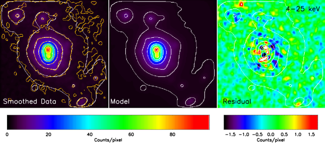
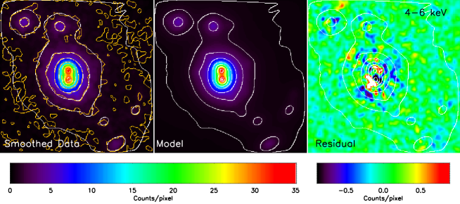
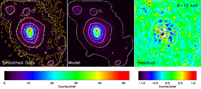
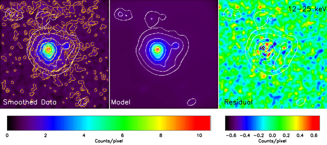
Figure 4.— PSF-convolved point source image fits – for the same region shown in Figure 3 – in four energy bands, from top to bottom: 4–25 keV, 4–6 keV, 6–12 keV, and 12–25 keV. In the leftmost panels, the image displays the smoothed, background-subtracted counts data from all 3 epochs, with the overlaid yellow contours following the data. The middle panels show the best-fit model (described in Section 4.1.1) with the same color scale as the data, and the white contours (also reproduced in the left and right panels) follow the underlying smoothed model image. In the right panels, the residual of the other two panels (data$-$model) is displayed with its own smaller and more refined color bar. All images have been smoothed by a Gaussian kernel of 2 pixels ($\sim 5$^′′), and the contours have square-root spacing between the minimum and maximum values of the model images; both the yellow (data) and model (white) contours follow identical intensities. In the left panels, note how well the white contours track the yellow contours, even where the signal-to-noise is only moderately high, which is only possible thanks to the excellent PSF calibration of the NuSTAR telescopes. The lack of significant structure in the residual images also demonstrates the success of the fitting process and suggests we have identified all detectable sources of emission in the central 7.4^′ (8.5 kpc) of NGC 253.

4.1. Point Source Properties

4.1.1 Source Identification

We assume detectable NuSTAR sources have Chandra counterparts, since the Chandra observations were constructed to exceed the 2–8 keV point source sensitivity of the NuSTAR observations. For point sources in a background-dominated regime, spatial resolution is the primary driver of sensitivity, and Chandra’s PSF is more than an order of magnitude smaller than that of NuSTAR. While NuSTAR’s larger effective area (a factor of $\sim 2$ at 5 keV) allows for a faster accumulation of source counts, those counts are spread over a much larger detector area, leading to a similarly high accumulation of background events. The roughly seven times longer NuSTAR exposure time helps to offset the increase in noise due to the background, and an isolated source is expected to be detected at nearly the same significance in these Chandra and NuSTAR observations. However, our sources are not isolated, especially considering the arcminute-scale wings of the PSF, which complicate the detection of fainter sources near brighter ones.

Initially, sources from the Chandra catalogs with the highest 4–6 keV count rates are included in image fits (see Section 3.4 for details) to the 4–25 keV NuSTAR image. We inspected the resulting residual NuSTAR images and added sources from the Chandra 2–8 keV band catalogs where any faint, underlying sources might improve the fit. In all fits, we also include a spatial model for diffuse thermal gas based on residual diffuse emission in a 3–7 keV Chandra image (see Section 4.2.1 for more details) to ensure point source count rates, especially in the 4–6 keV band, are not biased. Marginal sources were later removed from our source list if their rates in three NuSTAR sub-bands were all below a 90% confidence threshold. The final rates were found by refitting our four image bands (4–6 keV, 6–12 keV, 12–25 keV, and 4–25 keV) with the same culled list of 23 sources, which is provided in Table 4.1.1. ID numbers locate each source in Figure 3.

For comparison, in each Chandra epoch we detect 36 sources on average in the 2–7 keV band within our central region of interest. About two of our 23 sources do not correspond to a Chandra source in a given epoch, although every NuSTAR source has a Chandra counterpart in at least one epoch, as one would expect. Of the $\sim 15$ sources not detected by NuSTAR, four are near the brightest sources 1–4, half of the remaining Chandra sources are near to (and presumably fainter than) other detected sources, and the rest are more isolated but have the lowest Chandra rates. We therefore detect about two-thirds of the Chandra sources in our region of interest, with the majority of undetected sources missed due to confusion-related issues.

We demonstrate the reliability of the fits to each energy band image in Figure 4. The varying PSF shape is well modeled across the image (note in particular Source 7), and the residuals, while not entirely random, indicate that any systematic error induced by an erroneously modeled PSF shape is $<5$% based on the ratio of residual fluctuations (right panels) over the counts at similar locations (left panels). The true systematic uncertainty in the PSF shape is probably even smaller given the impact of statistical fluctuations on the residual images, but since simple photon statistics dominate our uncertainties, systematic uncertainties related to the model PSF are not considered further. While the wings of Sources 1–4 contribute a large fraction of photons to the locations of surrounding sources, the fact that the model (white) contours follow the data (yellow) contours so well suggests the surrounding source fluxes are not strongly biased.

As an additional check, we compare the Chandra and NuSTAR 4–6 keV rates in Figure 5. A source with a power law photon index of 2 should fall on the solid line, based on a PIMMS count rate conversion (that is rather insensitive to photon index in any case). The agreement is good, although a few sources lie somewhat off the line given their 90% error bars, most notably Source 1. The comparison is done for the combined data of all epochs, which are not perfectly simultaneous (Fig. 1), primarily because the NuSTAR observations are so much longer. For Source 1 in particular, the NuSTAR rate increases after the Chandra observation has completed in both Epochs 1 and 3; in Epoch 3 the rate grows monotonically over the NuSTAR observation. Additionally, the few faint sources with higher NuSTAR rates (near source 10 on the plot) may result from variability and/or Eddington bias, since that is near the detection limit for NuSTAR.

It should be noted that while the three bright nuclear sources (Sources 2, 3, and 4, which correspond to sources B, A and C, respectively, in Lehmer et al., 2013) are individually fit for, their $\sim 3\mbox{${}^{\prime\prime}$}$ separations are too small to cleanly separate them spatially with NuSTAR. In Lehmer et al. (2013), the variability of Source 2 between epochs was used to isolate its spectrum in the NuSTAR data; however, we cannot make use of this fact because all epochs have been combined. While the 4–6 keV rates seem reasonable for Sources 2–4, given the large errors on the NuSTAR count rates, only their summed emission should be considered robust.

Table 2NuSTAR and Chandra Properties of NuSTAR NGC 253 Point Sources

					Chandra	NuSTAR Count Rates					NuSTAR
			Alt.		Count Rate	S	M	H	Full Band	$L_{X}$	Hardness Ratios
	R.A.	Decl.	Name		4–6 keV	4–6 keV	6–12 keV	12–25 keV	4–25 keV	4–25 keV	(M-S)	(H-M)
ID	(J2000)	(J2000)			(10-4 cts s-1)	(10-4 cts s-1)	(10-4 cts s-1)	(10-4 cts s-1)	(10-4 cts s-1)	($10^{38}$ erg s-1)	(M+S)	(H+M)
1	11.88733	-25.296933	X33	X2	167.8 $\pm$ 6.6	187.0 $\pm$ 06.9	153.1 $\pm$ 06.9	010.1 $\pm$ 02.5	353.2 $\pm$ 10.8	20.48	-0.10${}^{+0.03}_{-0.03}$	-0.88${}^{+0.04}_{-0.05}$
2	11.88825	-25.288459	X34	X1	101.0 $\pm$ 4.6	087.2 $\pm$ 41.0	127.7 $\pm$ 34.5	047.5 $\pm$ 16.4	273.0 $\pm$ 37.1	15.83	00.19${}^{+0.24}_{-0.26}$	-0.46${}^{+0.23}_{-0.21}$
3	11.88740	-25.288848	X34	X1	033.5 $\pm$ 2.6	065.6 $\pm$ 31.5	099.0 $\pm$ 29.7	$<$28.5	172.0 $\pm$ 32.0	09.97	00.20${}^{+0.27}_{-0.26}$	$<$-0.50
4	11.88907	-25.289483	X34	X1	025.7 $\pm$ 2.3	025.9 $\pm$ 21.7	068.7 $\pm$ 24.3	$<$8.2	090.3 $\pm$ 30.7	05.23	00.45${}^{+0.36}_{-0.33}$	$<$-0.64
5	11.92817	-25.250640	X40	X6	032.5 $\pm$ 2.6	030.1 $\pm$ 02.8	024.0 $\pm$ 02.7	002.0 $\pm$ 01.4	057.8 $\pm$ 04.7	03.35	-0.11${}^{+0.07}_{-0.07}$	-0.84${}^{+0.12}_{-0.12}$
6	11.89680	-25.253328	X36	X4	045.4 $\pm$ 3.2	029.1 $\pm$ 01.7	016.8 $\pm$ 01.6	001.6 $\pm$ 01.1	048.4 $\pm$ 02.8	02.81	-0.27${}^{+0.05}_{-0.05}$	-0.83${}^{+0.10}_{-0.11}$
7	11.84415	-25.347447	X21	X9	022.6 $\pm$ 2.2	020.9 $\pm$ 01.7	020.7 $\pm$ 01.9	003.2 $\pm$ 01.5	046.9 $\pm$ 03.0	02.72	-0.00${}^{+0.06}_{-0.06}$	-0.73${}^{+0.10}_{-0.10}$
8	11.86456	-25.283152			003.0 $\pm$ 0.8	004.2 $\pm$ 01.4	011.2 $\pm$ 01.6	007.2 $\pm$ 01.4	022.3 $\pm$ 02.6	01.29	00.45${}^{+0.14}_{-0.14}$	-0.22${}^{+0.11}_{-0.12}$
9	11.89275	-25.284328			006.4 $\pm$ 1.2	012.8 $\pm$ 05.1	007.0 $\pm$ 05.3	$<$4.4	020.2 $\pm$ 08.3	01.17	-0.29${}^{+0.37}_{-0.37}$	$<$0.12
10	11.88968	-25.304607			002.1 $\pm$ 0.9	006.3 $\pm$ 03.6	011.1 $\pm$ 03.7	$<$2.6	019.1 $\pm$ 05.4	01.10	00.27${}^{+0.31}_{-0.30}$	$<$-0.44
11	11.87906	-25.307325	T		021.8 $\pm$ 2.7	005.7 $\pm$ 03.5	009.3 $\pm$ 03.7	003.3 $\pm$ 01.4	019.0 $\pm$ 05.7	01.10	00.24${}^{+0.34}_{-0.35}$	-0.47${}^{+0.28}_{-0.36}$
12	11.82706	-25.320597	X19	X8	011.5 $\pm$ 1.5	007.9 $\pm$ 01.5	008.5 $\pm$ 01.6	$<$0.6	017.3 $\pm$ 02.7	01.00	00.04${}^{+0.14}_{-0.13}$	$<$-0.78
13	11.90137	-25.277431			007.1 $\pm$ 1.2	006.9 $\pm$ 01.9	008.7 $\pm$ 02.1	$<$2.2	016.9 $\pm$ 03.4	00.98	00.11${}^{+0.18}_{-0.18}$	$<$-0.55
14	11.85494	-25.329321	X23	X5	007.2 $\pm$ 1.3	006.9 $\pm$ 01.3	007.5 $\pm$ 01.5	$<$2.0	015.8 $\pm$ 02.3	00.91	00.04${}^{+0.14}_{-0.13}$	$<$-0.57
15	11.87807	-25.312500			001.3 $\pm$ 0.6	006.2 $\pm$ 02.6	007.5 $\pm$ 02.8	$<$1.0	013.0 $\pm$ 04.2	00.76	00.10${}^{+0.28}_{-0.28}$	$<$-0.56
16	11.93685	-25.249135			001.6 $\pm$ 0.6	004.6 $\pm$ 01.8	005.0 $\pm$ 01.9	002.5 $\pm$ 01.4	012.2 $\pm$ 03.0	00.71	00.04${}^{+0.31}_{-0.34}$	-0.32${}^{+0.23}_{-0.42}$
17	11.86666	-25.305651	X25		008.7 $\pm$ 1.3	003.8 $\pm$ 01.7	006.6 $\pm$ 02.0	$<$2.2	011.4 $\pm$ 02.9	00.66	00.26${}^{+0.27}_{-0.25}$	$<$-0.49
18	11.90926	-25.291312			003.8 $\pm$ 1.0	005.4 $\pm$ 01.7	004.4 $\pm$ 01.8	$<$2.0	010.7 $\pm$ 02.7	00.62	-0.11${}^{+0.24}_{-0.25}$	-0.64${}^{+0.42}_{-0.35}$
19	11.88176	-25.251690	X29		002.2 $\pm$ 0.7	003.7 $\pm$ 01.2	006.1 $\pm$ 01.4	$<$1.5	010.3 $\pm$ 02.2	00.60	00.24${}^{+0.21}_{-0.20}$	$<$-0.52
20	11.86907	-25.323165			006.9 $\pm$ 1.2	004.2 $\pm$ 01.2	003.7 $\pm$ 01.4	$<$0.8	008.0 $\pm$ 02.3	00.47	-0.06${}^{+0.23}_{-0.24}$	$<$-0.54
21	11.82344	-25.307427	X18	X7	003.9 $\pm$ 0.9	004.5 $\pm$ 01.3	003.1 $\pm$ 01.5	$<$0.9	007.0 $\pm$ 02.4	00.41	-0.18${}^{+0.28}_{-0.27}$	$<$-0.60
22	11.92964	-25.256389	X42		004.8 $\pm$ 1.0	002.1 $\pm$ 02.1	004.3 $\pm$ 02.2	$<$0.8	005.2 $\pm$ 03.8	00.30	00.34${}^{+0.48}_{-0.48}$	$<$-0.45
23	11.90485	-25.333878			002.0 $\pm$ 0.6	$<$1.2	$<$3.2	001.9 $\pm$ 01.2	$<$6.1	$<$0.36	$<$1.0

Figure 5.— Count rates in the 4–6 keV band for the same sources in the merged Chandra and NuSTAR observations; error bars correspond to the 90% confidence interval. The diagonal line corresponds to the expected relation ($\sim 0.82$ NuSTAR counts for every Chandra count using HEASARC PIMMS), and sources are numbered as in Table 4.1.1. The excellent agreement between the two instruments indicates the methods outlined in Section 3 work well.

4.1.2 Q-like and Color-Color Diagrams

Hardness-intensity diagrams (also known as “q” or “turtle”-shaped diagrams) are a simple tool for classifying XRB states. We create hardness ratios from the rates in Table 4.1.1 and compare them to Galactic BH-XRBs in different states and to Galactic accreting pulsars. NuSTAR count rates for these Milky Way (MW) sources are derived from spectral model fits to RXTE PCA spectra (for details, see Kyanidis & Zezas, in prep.). We have adopted the three-energy band division (over the total range that we detect emission: $E\mathrel{\hbox to0.0pt{\lower 3.0pt\hbox{$\mathchar 536\relax$}\hss}\raise 2.0pt\hbox{$\mathchar 316\relax$}}25$ keV) that provides the best discrimination between different types of sources. Table 4.1.1 provides these rates for the soft (S: 4-6 keV), medium (M: 6-12 keV), and hard (H: 12-25 keV) bands. In Figures 6 and 7, we show the expected locus in the NuSTAR data for the hard, intermediate, and soft spectral states of BH XRBs with blue, green and red squares, respectively. We clearly see that both in the “q”-like and color-color diagrams, they follow the well established pattern from the RXTE results (e.g., Remillard & McClintock, 2006; Done et al., 2007). In addition, we include accreting pulsars (magenta squares), which show systematically harder spectra, and ULXs from the analysis of NuSTAR data of several sources (orange squares): Bachetti et al. (2013, NGC 1313 X-1 and X-2); Rana et al. (2014, IC 342 X-1 and X2); Walton et al. (2014, Holmberg IX X-1); and Walton et al. (2013, the ULX in Circinus). Note that the ULX sources appear to have colors similar to intermediate state Galactic black holes but at much higher luminosities.

The NuSTAR sources from NGC 253 are overplotted on Figures 6 and 7 with black diamonds. Sources 1–4 fall within the ULX locus, and the next brightest sources (5–7) lie in between the ULX and intermediate state populations. The large degree of scatter seen in the models for the MW sources is the result of (a) distance uncertainties and (b) hysteresis effects (e.g., Maccarone & Coppi, 2003; Done et al., 2007), which may also account for the factor of $\sim 2$–3 offset between Sources 5–7 and the majority of MW rates. Also, estimates of the distance to NGC 253 itself are uncertain; we assume a distance 3.94 Mpc (Karachentsev et al., 2003), but other estimates place the galaxy much closer (e.g., 2.58 Mpc, Puche & Carignan, 1988), which would increase the predicted rates of the MW sources in Figure 6 by up to a factor of 2. Therefore, this separation does not necessarily imply that they are ULXs, although note that Sources 6 and 7 are considered to be ULXs by Kajava & Poutanen (2009). Alternatively, the fact that Sources 5–7 are systematically more luminous than the MW BH binaries used to construct the diagnostic diagram could be the result of the much younger populations present in NGC 253, which would result in generally more luminous XRBs (e.g., Fragos et al., 2013). Such sources, consisting of a massive BH accreting from a young massive star, are short lived and very rare in our Galaxy. The color-color diagram (Fig. 7) shows their consistency with intermediate (or, in the case of Source 6, soft) state sources as well as with ULXs. Note, however, that a high-mass donor is not strictly necessary to produce a high luminosity XRB (see, eg., Portegies Zwart et al., 2004; van Haaften et al., 2012).

The remaining 13 sources, which fall within our diagnostic luminosity range, are near the detection limit. Even so, they align most with the loci of intermediate and hard state BH binaries. The lack of soft state sources may be partially a selection effect, since the effective area peaks in the medium band. However, over the full band we are clearly able to detect sources down to a flux level where sources in the soft state would be apparent, implying most of the brightest binaries in NGC 253 are not in the soft state. We cannot conclude more generally about the soft state population as a whole, however, since we only consider those sources bright enough to have detectable emission in NuSTAR’s 4–6 keV band. In general, we are likely catching these sources as they brighten in the hard state and pass for the first time into the intermediate state, before they continue into the soft state and fade. The state of any individual source is unclear, given color uncertainties and imperfect segregation of states on the diagrams.

The one exception to this is Source 8, which falls within the pulsar locus in both diagrams. Its hard spectrum, obvious from both Figures 3 and 7, makes it an ideal source for study with NuSTAR despite its low 4–6 keV flux, thanks to the flat/rising NuSTAR effective area up to $\sim 12$ keV.

4.1.3 NGC 253 Spectrum

Although NuSTAR is the first observatory to resolve NGC 253 into individual components at energies above $E\sim 10$ keV, spatial crosstalk between many of the sources complicates their spectral analysis. Figure 14 presents spectra extracted at the location of 6 different sources to show their relative contribution and signal-to-noise at higher energies. The size of the circular extraction regions for each spectrum are given in the figure. The “Total Galaxy” spectrum is extracted from a much larger aperture (4.5^′  radius circle with the areas beyond the $D_{25}$ radius to the northwest and southeast excluded); the larger detector area encompassed in the region includes proportionately more background that degrades the signal-to-noise, especially at higher energies. Above $\sim 10$ keV, nearly all of the emission falls within 100^′′  of the galactic center and is produced almost entirely by Sources 1–4 and Source 8 (at the highest energies). This spectrum is extremely well fit by a broken power law with a single Gaussian component to account for the Fe-K emission, across the entire energy range over which counts are detected: 3–40 keV (with $n_{H}$ fixed at the Galactic value). In line with other ULX spectra, the high energy emission is soft, with steep photon indices both below ($2.36\pm 0.06$) and above ($3.14\pm 0.06$) the break energy of $5.7\pm 0.3$ keV. This result is consistent with the “q”-like and color-color diagram results given that Source 1 and most if not all of the nuclear sources fall within the ULX locus of Figure 6.

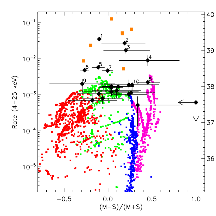
Figure 6.— Hardness-intensity or “q”-like diagram for our sources (black diamonds with 90% error bars or upper limits). The hardness ratio is derived from the rates in the medium (M: 6–12 keV) and soft (S: 4–6 keV) bands. The 10 brightest 4–25 keV sources are labeled as in Table 4.1.1. Other binary types/states are depicted as squares with the following colors: orange: ULX sources; magenta: accreting pulsars; blue: hard state BH XRBs; green: intermediate state BH XRBs; and red: soft state BH XRBs (see Section 4.1.2 for details). The ULXs are taken from other NuSTAR observations (references in the text), while the other symbols are derived from RXTE observations of Milky Way binaries. Count rates for these objects and luminosities for our sources are estimated using a distance of 3.94 Mpc.

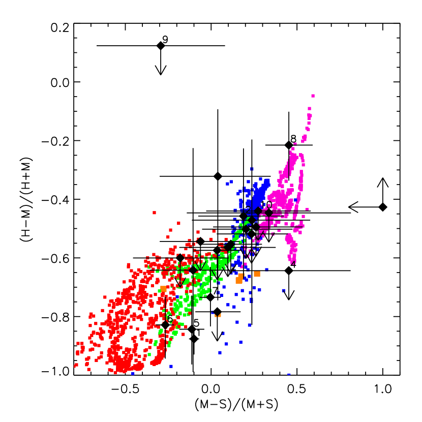
Figure 7.— Color-color diagram for our NuSTAR sources. The symbols are the same as in Figure 6, and in this diagram we also utilize the hard (H: 12–25 keV) band count rates. Although uncertainties are large, the sources fall on the expected loci for BH XRBs. The pulsar candidate, Source 8, is well separated from other binary accretion modes.

We also see that the nuclear region is much harder than many of the other sources and is clearly where the Fe-K line complex originates. To first order, the overall spectrum appears dominated by a few bright sources that are soft, with an equivalent photon index $\Gamma>2$.

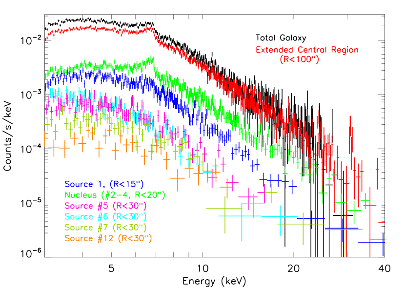
Figure 8.— Total NGC 253 NuSTAR spectrum (black) within $D_{25}$ relative to the spectra of the brightest individual sources contributing to the total spectrum. The nuclear point source emission (Sources 2–4) is shown in green and that from Source 1 in blue. The emission is clearly dominated by the inner 100^′′of the galaxy, and we find that $>99$% of the hard X-ray flux is attributed to resolved point sources. The extended central region spectrum is fit well by a broken power law model with a steep photon index of $3.14\pm 0.06$ above $\sim 6$ keV up to 40 keV, as described in Section 4.1.3. This region contains nearly all of the $E>10$ keV emission from NGC 253; the other sources contribute primarily to the spectrum at lower energies.

An exception is Source 8, the pulsar candidate, which has a very flat spectrum ($\Gamma\sim 1$, see Section 5.2). Such a hard spectrum could also be produced by a background AGN and just happen to fall within the pulsar loci of Figures 6 and 7. If so, one might expect it to have an optical counterpart. Cursory inspection of F850LP, F606W, and F475W HST ACS images at the location of Source 8 failed to reveal any obvious counterparts. While insufficient to rule out the classification of the source as an AGN, this fact does bolster the pulsar interpretation. Because the spectra of Sources 1–4 fall off much faster above 10 keV ($\Gamma\mathrel{\hbox to0.0pt{\lower 3.0pt\hbox{$\mathchar 536\relax$}\hss}\raise 2.0pt\hbox{$\mathchar 318\relax$}}3$), Source 8 makes up about 20% of NGC 253’s total emissivity at 20 keV. Other fainter but similarly hard point sources may lurk within the PSF wings of Sources 1–4 and thus go undetected. If so, such sources might contribute significantly to the $E>20$ keV spectrum of starburst galaxies generally.

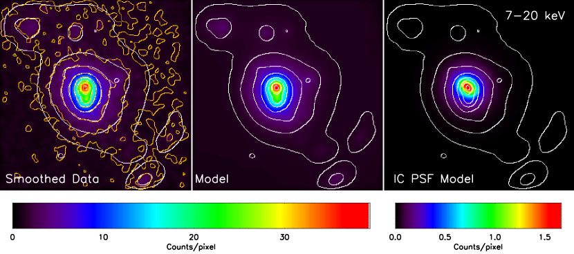
Figure 9.— Point source fit to the data in the 7–20 keV band used for setting limits to the IC flux associated with the starburst (details of the left and middle panels are the same as in Figure 4). In the right panel, we show the PSF-convolved spatial model for IC emission, assuming a 20^′′$\times$4^′′  ellipse of constant surface brightness, scaled to the expected flux in the leptonic models of Lacki & Thompson (2013). The elliptical projected shape for the diffuse emission allows it to be distinguished from the bright nuclear point sources despite being co-located with them. The leverage gained from imaging the starburst region, made possible by NuSTAR, allows us to set the deepest limits on IC emission in NGC 253 to date.

4.2. Constraints on Unresolved/Diffuse Emission

There are three likely sources of diffuse emission: truly diffuse thermal emission, truly diffuse non-thermal emission, and unresolved XRBs. The thermal gas is very soft, with $kT\mathrel{\hbox to0.0pt{\lower 3.0pt\hbox{$\mathchar 536\relax$}\hss}\raise 2.0pt\hbox{$\mathchar 316\relax$}}1$ keV, and will contribute only at the lowest NuSTAR energies, if at all. Non-thermal emission is most likely to originate from cosmic-ray electrons IC scattering the intense FIR radiation field in the starburst to X-ray and $\gamma$-ray energies. This emission should be present at some level throughout the NuSTAR band, due to its hard ($\Gamma\sim 1.6$) spectrum. Unresolved binaries, however, will be difficult to distinguish from the nuclear sources given the spatial resolution of NuSTAR. Otherwise they will be confused with the emission from Sources 2-4 or with an IC component, which is assumed to have a spatial distribution similar in size to the starburst region.

4.2.1 Contribution of Unresolved Point Sources and Diffuse Gas

An unresolved XRB population is likely brightest in the nucleus, enhanced by HMXBs resulting from the intense star formation there, where it is confused with Sources 2–4. These three sources are separated by several arcseconds, so given the large NuSTAR PSF, a peaky spatial distribution of binaries within the central $\sim 75\mbox{${}^{\prime\prime}$}-100$^′′ would be impossible to distinguish from the bright nuclear sources. A slightly more extended population distributed across the entire starburst region or beyond could be detectable, but given the results of the next subsection (4.2.2), we can only set upper limits on the flux of an unresolved binary component.

The diffuse thermal gas, although soft ($\sim 1$ keV in the hot outflow, e.g., Strickland et al., 2000; Mitsuishi et al., 2013), may bias fits in the lowest energy bands if no spatial model is included for its contribution. From the 3–7 keV Chandra image, we construct a template surface brightness map, excluding point sources, that is convolved with the NuSTAR PSF to account for its emission. While included in fits to all energy bands, as expected this component is only even potentially present in the 4–6 keV band; its best-fit value is $\sim 1$% of the combined flux of the 3 nuclear sources. It is not formally detected at the 90% confidence level. Its morphology primarily follows the outflow to the southeast, which differs from the other components significantly enough that we therefore expect no bias from thermal emission in any of our results.

Table 3Inverse Compton 90% Upper Limits

Projected	Semi-major/minor	Upper Limit	$\nu F_{\nu}(20~{}{\rm keV})\tablenotemark{b}$
Shape	axes or Radius	($10^{-14}$ ergs s-1 cm-2)
Ellipse	20′′$\times$4′′	14.2	16.6
Ellipse	40′′$\times$8′′	11.8	13.8
Ellipse	60′′$\times$12′′	08.7	10.1
Circle	15′′	17.7	20.7
Circle	30′′	06.5	07.6
Circle	45′′	03.1	03.7
Circle	60′′	02.4	02.8

4.2.2 Inverse Compton Emission

Because NuSTAR is the first observatory able to resolve non-nuclear sources away from the central starburst at $E\mathrel{\hbox to0.0pt{\lower 3.0pt\hbox{$\mathchar 536\relax$}\hss}\raise 2.0pt\hbox{$\mathchar 318\relax$}}10$ keV, we have the capability to determine whether any of the emission is both non-thermal and diffuse. The clean residuals for the 12–25 keV band in Figure 4 already suggest that a detection of non-thermal IC emission cannot be claimed. However, we can place the tightest limits yet on an IC component associated with the starburst in NGC 253, which further constrains the physical mechanisms producing the $\gamma$-ray emission in the galaxy.

Selecting an optimal energy band for constraining the IC component requires maximizing the signal-to-noise ratio, where the noise is contributed by both the background and resolved sources of emission. Since the IC component is predicted to be relatively hard (e.g., Lacki et al., 2012), we adopt a lower energy threshold of 7 keV to minimize soft-spectrum contributions from diffuse thermal emission (also avoiding the Fe-K line complex around 6.5–7 keV) and individual sources, many of which have spectral breaks near this energy. At the high-energy end, we encounter the relatively flat-spectrum instrumental background and the signal-to-noise degrades. More precisely, the background decreases with energy up to $E\sim 20$ keV, where we encounter a complex of strong fluorescence lines. Given these observational conditions, we restrict ourselves to the 7–20 keV band.

Assuming IC emission originates from a disk-like region coincident with the central starburst as in, e.g., Lacki & Thompson (2013), we expect a highly elliptical IC surface brightness due to the large inclination of the galaxy. This distinct appearance allows the spatial dimension to be more constraining than the spectral dimension. The uncertainty in the hard-band spectral indices of the 3 nuclear sources is large, so a larger IC flux is allowed in spectral fits because the model for the point source spectra will simply become steeper as the IC flux increases. In contrast, spatial fits better avoid confusion between the IC and point source components. Figure 9 shows the point-source fit to the data in the 7–20 keV image in the left and center panels, just as in those panels in Figure 4. We do not include the diffuse component meant to represent thermal gas since its flux was consistent with zero in the 6–12 keV and 12–25 keV band fits.

To determine the 90% upper limit on the IC component, we added an extended, PSF-convolved IC component to the best-fit spatial model of the point-source population. We varied its size and intensity until C-stat increased by an additional 2.706 above its value without the IC component. The right panel in Figure 9 shows a sample PSF-convolved IC model with an assumed 20^′′$\times$4^′′  ellipse of constant surface brightness. The total flux displayed in this spatial model is roughly consistent with the predicted value in the leptonic models of Lacki & Thompson (2013), which amounts to $\sim 5$% of the total nuclear emission. Our upper limit for this model is $\sim 2$ times brighter.

In Table 3, we list upper limits for a variety of simple IC geometries. Perhaps counterintuitively, the upper limits become more stringent as the region increases in size, despite the fact that the IC surface brightness decreases with the size of the region for a given flux (i.e., the same flux is spread over a larger area). This trend is a direct result of the degeneracy between more compact diffuse regions and the nuclear point sources. The smaller IC regions are closer in size to the NuSTAR PSF, so that as the diffuse IC flux is increased when deriving upper limits, the flux in the point sources can correspondingly decrease to maintain a reasonable fit. When the IC region size becomes much larger than the PSF FWHM, however, the flux from point sources cannot compensate as well, resulting in lower flux limits despite the fact that the IC flux is spread over a larger area. In other words, our sensitivity to IC emission is dominated by the degeneracy between the nuclear point source fluxes and the IC flux.

5. X-ray and Radio Variability

We repeated the image analysis on each epoch individually, allowing the detection of month-scale variability from state changes in the brightest sources. Considering the epochs separately also allows more physically meaningful joint Chandra-NuSTAR spectral fits of those sources.

Table 4Per Epoch Corrected Count Rates of NuSTAR NGC 253 Point Sources

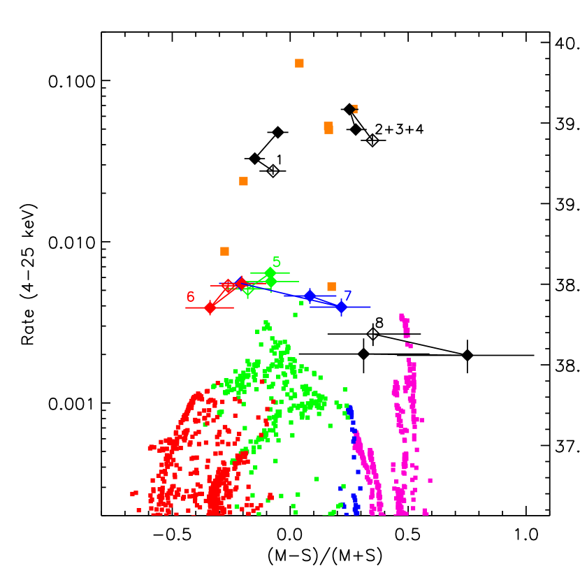
Figure 10.— Hardness-intensity or “q-like” diagram for the brightest 8 sources in each epoch (black and color diamonds with 90% error bars; upper limits are shown with error bars extending to values of 1.0). The first epoch is indicated by an open diamond. The symbols and band definitions are the same as in Figure 6, and the sources are labeled as in Table 4.1.1. While some significant variability in overall flux is seen in a few sources, only Source 7 undergoes a significant change in hardness ratio, indicative of a state change.

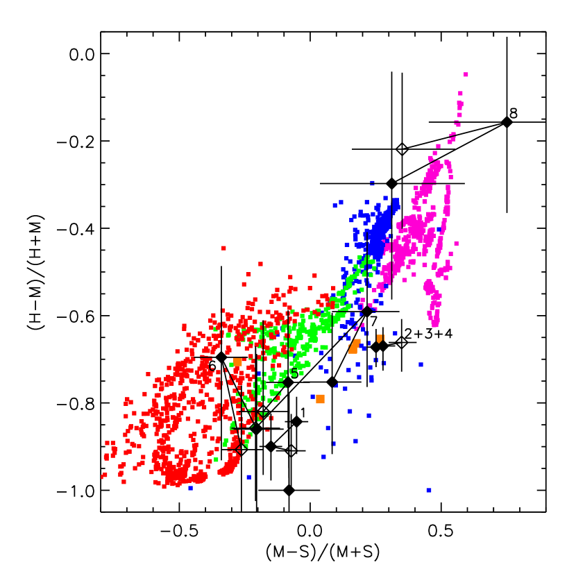
Figure 11.— Color-color diagram for the brightest 8 NuSTAR sources in each epoch. The symbols are the same as in Figure 10, and error bars that reach 1.0 or $-1.0$ are really upper or lower limits, respectively. Although uncertainties are large, the “color” of Source 7 evolves from that of a soft or intermediate state (red/green) to the hard state (blue).

5.1. Image Fits

The lower per-epoch depths limits us to the brightest $\sim 8$ sources for discerning state changes between epochs. Because the nuclear sources (2, 3, and 4) are confused in the NuSTAR data, we previously used variability – shown to be caused primarily by only Source 2 – to investigate their characteristics (Lehmer et al., 2013). Given this work, we focus on the nature of the other 5 sources.

In general, each source undergoes some marginally statistically significant variation between epochs, although largely in overall luminosity and not color. From Epochs 1–3, Source 1 steadily increases in flux, Sources 5 and 6 exhibit slight negative fluctuations in the second epoch, and Source 8 may have also dropped in flux after the first epoch. The only source to experience a clear color change is Source 7; its 4–6 keV count rate is $\sim 2$ times brighter in the first epoch than in the other two epochs while its $\mathrel{\hbox to0.0pt{\lower 3.0pt\hbox{$\mathchar 536\relax$}\hss}\raise 2.0pt\hbox{$\mathchar 318\relax$}}7$ keV emission remains unchanged. Table 5 gives the count rates for each source and Figures 10 and 11 place these count rates on the state diagnostic diagrams.

The hardening of Source 7 is apparent in Figure 10, which suggests either a transition from the soft to hard state or oscillations between soft and intermediate states (that create the “eye of the turtle” in the “q” diagram, e.g., Fender et al., 2004). The latter interpretation is more likely given that it occurs at higher luminosities and that soft-to-hard transitions generally occur at $\sim 2$% of the Eddington luminosity (Maccarone, 2003). In Figure 11, the hard band colors largely bolster this interpretation, although the colors are also consistent with the hard state, given the uncertainties. Modeling the detailed spectra may be able to constrain whether the emission is disk-dominated or not, and therefore confirm source states. Although the results of these fits may not directly correspond to state changes in “q”-like diagrams (e.g., Dunn et al., 2010), we nevertheless apply simple models to our spectra in Section 5.2.

5.2. Joint Chandra-NuSTAR Fits to Brightest Sources

Assuming variability on short (day-long) timescales is minimal, the near simultaneous Chandra and NuSTAR spectra can be fit together over a broad (0.5 keV $<E<$ 25 keV) energy range. Narrow energy ranges can fail to discriminate between non-thermal and thermal-dominated spectra due to degeneracies between highly absorbed power law and multi-color blackbody disk (MCD) spectral shapes. Typical disk models peak in energy output around $\sim 2$–3 keV, so coverage well beyond 3 keV is necessary to determine whether the curvature observed below 3 keV is truly thermal and not just the result of a large absorbing column.

Because of low signal-to-noise above 10 keV, we only consider simple non-thermal (POWERLAW) and thermal (DISKBB, Makishima et al., 1986) XSpec spectral models, which are fit separately in an attempt only to determine which component dominates. In reality, most of our spectra are a mix of the two, with some fraction of the disk Comptonized into a non-thermal corona. A generic and self-consistent modeling of this scenario – convolving the disk emission with a Comptonization model, e.g., SIMPL$\ast$DISKBB in XSpec as demonstrated in Steiner et al. (2009) – unfortunately leads to unphysical results. Even our disk-dominated sources exhibit slight excess emission above 10 keV, but the fit pushes the composite model to complete Comptonization with a power law component that is too steep ($\Gamma>4$). Because the energy range is still too low to see the non-thermal component dominate the emission anywhere, degeneracies between absorption, the disk innermost radius temperature, and non-thermal index produce uninteresting results.

Due to the proximity of the sources ($\sim 1\mbox{${}^{\prime}$}$ separations), cross-contamination of the NuSTAR spectra from the PSF wings of other sources is inevitable. To counter this difficulty, we extract spectra in circular regions encompassing only 20–50% of the total emission (15–30^′′ in radius) and jointly fit all 8 sources with generic broken power-law models to approximate each source’s spectrum. When a single source is later modeled in detail, the contribution of other sources to the NuSTAR spectrum are included as a contamination model. The contamination contribution is sub-dominant for all sources except Source 8, which is intrinsically faint and resides nearest to Sources 1–4.

The POWERLAW and DISKBB best-fit parameters for each epoch and source are given in Table 5.2. For the soft and intermediate state sources (1, 5, and 6), the disk model generally is a better description of the data. The model is only really sufficient for Source 1, however; Sources 5 and 6 have moderate to significant excesses at $E>10$ keV. These sources are likely to be in an intermediate or possibly a steep power law state.

Table 5Joint Chandra-NuSTAR Spectral Fits

.

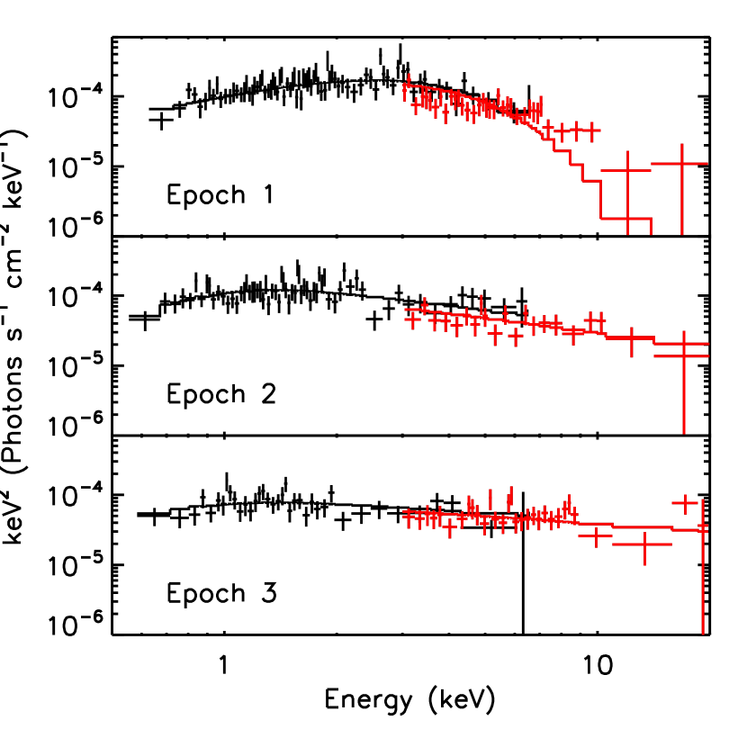
Figure 12.— Source 7 Chandra and NuSTAR spectra fit to the DISKBB (Epoch 1) or POWERLAW (Epochs 2 and 3) models. Over the course of the observations, the spectrum hardens, primarily due to a loss of flux below $\sim 8$ keV, likely the result of a diminishing disk component.

Source 7, while statistically preferring the non-thermal model, is better described as becoming more non-thermal over the course of the observations (Fig. 12). During the first epoch, its spectrum looks much like that of Source 5, consistent with a highly absorbed steep power law ($\Gamma=3.0\pm 0.1$), where the model parameters mimic a hybrid thermal/non-thermal shape and do not represent true physical conditions in the system. In the subsequent epochs, the spectrum hardens and the disk contribution generally diminishes, as evidenced by that hardening and the falling value of $n_{\rm H}$. The application of more complicated models would be necessary to physically interpret the transition, but this is not warranted by the signal-to-noise of the spectra. However, the spectral fits provide further evidence that Source 7 is transitioning to the intermediate state. Its Epoch 3, 2–7 keV Chandra count rate is approaching the lowest value measured across all archival Chandra observations since 2000, consistent with soft-to-intermediate state movement on the upper left part of the “q”-like diagram (Fender et al., 2004).

Source 8, unlike all of the other sources, clearly has a hard spectrum. Although both models appear to describe the spectra almost equally well, the disk inner radius temperature would have to be atypically high. The hard ($\Gamma\sim 1$) spectrum is consistent with other accreting pulsars in outburst (e.g., Miyasaka et al., 2013), but the source is too faint to see the typical high energy ($E\mathrel{\hbox to0.0pt{\lower 3.0pt\hbox{$\mathchar 536\relax$}\hss}\raise 2.0pt\hbox{$\mathchar 318\relax$}}20$ keV) curvature if it is an accreting pulsar. Archival Chandra data reveal that Source 8 is roughly persistent, exhibiting little to no variability between the 5 observations over 12 years in which it could have been detected. The lack of variability argues against it being a transient Be/XRB, unless it is continually outbursting.

We also investigated the long term Chandra variability of all of our sources. In general, the brighter sources exhibit some variation in their 2–7 keV count rates, while fainter sources lack photon statistics necessary for variability constraints. Only two sources (15 and 18) are clear transients, having been detected for the first time in these observations. Source 15 is detected in Epoch 3 alone, and Source 18 is undetected in the first epoch but is growing in flux from Epoch 2 to 3. The uncertainty in their NuSTAR measurements, however, precludes us from concluding anything about their nature based on hard energy data.

5.3. Radio Monitoring

The VLBA campaign was intended to catch flares of similar intensity to those observed in Cyg X-3. In individual epochs, no flares were detected above our rms ($1\sigma$) noise of $\sim$150 $\mu$Jy beam^-1.

Within the core of NGC 253, we detect the two brightest known VLBI SN remnants, but no new sources were detected. This is not surprising since: (1) most radio sources in the cores of starburst galaxies are diffuse Hii regions or supernova remnants (e.g., in M82: McDonald et al., 2002; Gendre et al., 2013) and at typical expansion speeds of 10,000 km s^-1 would be resolved out by the VLBA after 300 years; (2) there is significant free-free absorption towards the core of NGC 253 (e.g., Tingay, 2004; Lenc & Tingay, 2006; Rampadarath et al., 2014); (3) the predicted supernova rate is low ($<0.2$ yr^-1; Rampadarath et al., 2014); and (4) there is no radio evidence for an AGN (Brunthaler et al., 2009). In the wider galaxy, the lack of detections corresponding to the Chandra and NuSTAR sources is also not surprising given the probability of catching a flare, but we are able to put a limit on their radio brightness at the time of observation. For phase centers correlated in all three epochs, the rms in the images made from combining all three epochs is $\sim$65 $\mu$Jy beam^-1. At a distance of 3.94 Mpc, this puts a $5\sigma$ limit of $6\times 10^{17}$ W Hz^-1 on the brightness of individual counterparts.

6. Discussion

6.1. Extragalactic Point Sources at Hard Energies

We present the first imaging observations above 10 keV for a galaxy outside the Local Group. For the first time, we are able to spatially resolve the $>10$ keV X-ray emission of NGC 253 into individual sources, revealing that the galaxy’s overall spectrum turns over (is relatively X-ray soft) above 10 keV and is dominated by a small number of luminous sources that also show turnovers above 10 keV. Source rates and colors (i.e., hardness ratios) are used to characterize source types through diagnostic plots, in which the spectra of MW BH binaries have been translated into NuSTAR rates and colors.

Comparison of MW binaries to our sources suggests that the majority (by number) of the NGC 253 XRB population are black holes primarily in the intermediate and possibly hard state, which is dominated by a power-law/non-thermal component. Since observations of external galaxies give us a view of the entire galaxy simultaneously, we can effectively constrain the dominant states of all binaries at several snapshots in time. Direct comparison of the near-Eddington accreting sources we detect in the MW is problematic; as is clear from Figure 6, we hit our detection threshold roughly where we expect the brightest MW binaries to be. Only a single XRB in the Milky Way, GRS 1915+105, has spent long periods of time with an X-ray luminosity at or near the Eddington luminosity. Reig et al. (2003) examined a large number of observations, and concluded that GRS 1915+105 is nearly always in the “very high state,” consistent with the bright intermediate state. Some sources may be expected to be caught in extremely bright hard states as transients (e.g., V404 Cyg, Oosterbroek et al., 1998).

We also find one source, 8, that may be an accreting pulsar based on its position in the hardness/intensity diagrams (Figs. 6 and 7). Given the short duration of the type-I outbursts (associated with neutron stars) of Be XRBs, and the very rare occurrence of the more energetic type-II outbursts (e.g., Reig, 2011), we would not expect a very large number of these systems in the few snapshots we have obtained. Source 8, however, is persistent, having been detected in all sufficiently sensitive Chandra observations at roughly the same flux. This persistence suggests we have not observed a single long or multiple $L_{X}\sim 10^{38}$ erg s^-1 outbursts, but instead an extremely X-ray luminous pulsar. Because the source is faint and seemingly heavily absorbed, the intrinsic spectrum may not be as hard as observed. In this case, the actual accreting object may be a stellar-mass BH XRB or an obscured AGN behind the galaxy.

Interestingly, the most luminous NuSTAR sources in NGC 253 (including the most luminous source in the neighborhood of the nucleus; Lehmer et al., 2013) are located in the region of color-intensity (“q”-like) and color-color diagrams occupied by NuSTAR-observed ULXs. Sources 6 and 7 have in fact been considered ULXs in a previous study (Kajava & Poutanen, 2009). Unlike Source 1, a clear ULX in all of our observations, the spectra of Sources 5–7 favor a hard non-thermal component in addition to the thermal component, which strongly dominates NuSTAR-observed ULXs (e.g., Bachetti et al., 2013; Walton et al., 2013; Rana et al., 2014; Walton et al., 2014). Their variability over the past 12 years, however, suggests they may very well exhibit ULX-like luminosities, even if they appear as borderline ULX candidates in these observations.

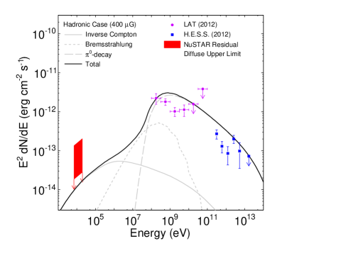
Figure 13.— Broadband (X-ray to $\gamma$-ray) modeling of cosmic ray emission mechanisms under leptonic (left panel) and hadronic (right panel) scenarios, using the model parameters of Lacki et al. (2012), which are based on the the GeV (Fermi LAT, Ackermann et al., 2012) and TeV (H.E.S.S., Abramowski et al., 2012) detections of NGC 253. The range of upper limits at X-ray energies provided by NuSTAR are given by the red/shaded box (see Table 3 for numerical values and corresponding emission region sizes). Although typical leptonic models are ruled out for large IC emitting regions, small regions confined to the starburst itself are allowed by these NuSTAR constraints.

6.2. Constraints on Non-thermal Emission

The spatial resolution and effective area at $E>10$ keV provided by NuSTAR has allowed the most sensitive constraint on IC emission in a starburst galaxy to date. In Section 4.2.2, we derive upper limits for various assumptions of the spatial distributions of the IC-emission. Although we are not quite able to use the upper limits to discriminate between the leptonic and hadronic scenarios that can both describe the $\gamma$-ray emission from NGC 253, we consider each scenario in comparison to our results.

The evolution of cosmic-ray nuclei and electrons is determined by the diffusion-loss equation (see, e.g., Longair, 1994):

$$-D\nabla^{2}N(E)+\frac{N(E)}{\tau(E)}-\frac{d}{dE}\left[b(E)N(E)\right]-Q(E)=-\frac{\partial N(E)}{\partial t}\,,$$ (1)

where $D$ is the scalar diffusion coefficient, $\tau(E)$ is the timescale for particles with energy $E$ to escape the region, $b(E)$ is the cooling rate for the particles, $Q(E)$ is the source term, and $N(E)$ is the number density of particles with energies in the range $E$ and $E+dE$. In our modeling, we assume that the system is in steady state ($\partial N(E)/\partial t=0$) and that the spatial dependence of the diffusion term can be neglected ($D\nabla^{2}N(E)=0$). Equation 1 can be solved using the Green’s function (Torres et al., 2004)

$$G(E,E^{\prime})=\frac{1}{b(E)}\exp\left(-\int_{E}^{E^{\prime}}dy\frac{1}{\tau(y)b(y)}\right)\,,$$ (2)

which for a given source term, $Q(E)$, results in the steady-state solution given by

$$N(E)=\int_{E}^{E_{\rm max}}dE^{\prime}Q(E)G(E,E^{\prime})\,.$$ (3)

From this particle distribution, we can compute the broadband non-thermal diffuse emission by convolving with the spectra of the various cooling interactions and the target particles.

In the case of cosmic-ray nuclei, the non-thermal diffuse emission predominantly at $E\mathrel{\hbox to0.0pt{\lower 3.0pt\hbox{$\mathchar 536\relax$}\hss}\raise 2.0pt\hbox{$\mathchar 318\relax$}}100$ MeV arises from pion production interactions with interstellar gas. In the case of cosmic-ray electrons and positrons, the emission extends from X-rays through GeV $\gamma$-rays and arises from bremsstrahlung interactions with interstellar gas and IC scattering of interstellar radiation. These interactions are also included in the cooling rates, $b(E)$, for the various particle species. We also account for cooling due to ionization (for all cosmic-ray species) and synchrotron (electrons and positrons). Additional losses due to particle escape ($\tau(E)$) via diffusion and/or advection due to starburst winds are included in the model. For positrons, annihilation is included as an additional escape term. Primary particles ($Q(E)$) are assumed to be accelerated in supernova remnants, and are injected with power-law spectra ($\Gamma\sim 2.1$; see Lacki et al., 2012; Chakraborty & Fields, 2013). Secondary electrons and positrons from pion-production (computed using the analytical formulae from Kelner et al., 2006) and from ionization by cosmic-ray nuclei are included in the electron source term for computation of the final electron/positron distributions. The final broadband diffuse spectrum is calculated assuming the best-fit physical parameters (i.e., supernova rate, acceleration efficiencies, galaxy gas mass, starburst wind speed, diffusion timescales, and region sizes) for the leptonic ($B\sim 50\mu$G) and hadronic ($B\sim 400\mu$G) models in Lacki et al. (2012, see their Table 1). However, for the interstellar radiation field (the seed photons for the IC emission), we adopt the radiative transfer model from Siebenmorgen & Krügel (2007). Viable diffuse models are required to reproduce both the Fermi-LAT (Ackermann et al., 2012) and H.E.S.S. (Abramowski et al., 2012) data points.

In Figure 13, we plot two models (one in each panel) for the $\gamma$-ray emission in NGC 253 under scenarios in which the emission is dominated either by leptonic or hadronic processes. To match the GeV and TeV observations, different assumptions of the cosmic-ray density and magnetic field strength are made in each case. The leptonic model (left panel) results in much more non-thermal emission in the hard X-ray band than in the hadronic model (right panel). In both panels, the NuSTAR upper limits on the broadband diffuse component for various assumptions about the size of the emission region are given by the shaded region. As the dense gas and radiation environment of the starburst is expected to prevent electrons from diffusing too far in the disk of the galaxy, the size of the emission region is expected to be roughly the size of the starburst core ($R\sim 350$ pc), which roughly corresponds to an angular size of $\sim 20\mbox{${}^{\prime\prime}$}$. The corresponding NuSTAR upper limits – the upper part of the shaded bands in Figure 13 – are comparable to the hard X-ray diffuse emission in the leptonic scenario, although larger emission region size estimates yield more stringent constraints. Hadronic models, on the other hand, have substantially less hard X-ray emission, and thus are out of reach for even the most optimistic size estimates.

Further modeling efforts regarding the spatial and spectral properties of the IC component (beyond the scope of this work) are needed to fully interpret the NuSTAR observations of NGC 253. Population synthesis models to account for individual sources too faint to be individually detected in the NuSTAR band would also enable more sensitive constraints on the IC emission; XRBs are expected to dominate the emission in low redshift star-forming galaxies (Lehmer et al., 2010; Schober et al., 2014). Still, the present constraints generally disfavor scenarios in which the $\gamma$-ray luminosity is attributed primarily to leptonic processes, providing further support for enhanced cosmic-ray energy density associated with actively star-forming environments.

6.3. The Global 0.5-40 keV Spectrum

To place these NuSTAR results a broader context, we construct and model Chandra and NuSTAR spectra for the entire NGC 253 galaxy. For the Chandra response files, RMFs and ARFs are weighted by the spatial distribution of emission, an approximation that works well given its concentrated PSF. The NuSTAR emission, entirely made up of what can effectively be considered point sources, is much less localized due to the larger PSF, making it inaccurate to simply weight the response files by the emission distribution in the same way. Instead, we assume all of the emission originates from the positions of the sources in Table 3, weighted by their relative 4–25 keV count rates, to construct an average ARF for use with the global spectrum.

While the contributors to the NuSTAR spectrum are effectively point-like, at lower energies thermal gas quickly dominates the global X-ray spectrum. Using the unresolved Chandra emission as a guide, we model it as a three-temperature plasma representing disk (cooler) and wind (hotter) gas: (1) an unabsorbed 0.3 keV component representing higher radius disk and halo gas, (2) a moderately absorbed 0.6 keV component representing warmer disk and the large-scale wind emission, and (3) a highly absorbed 2 keV component representing superwind emission associated with the nuclear starburst. The latter component is confined to within the nuclear starburst region, whereas the cooler gas components are much more extended. The remaining detected emission is entirely from point sources, which we model as a broken power law with best-fitting indices of 1.5 and 3 below and above, respectively, the break energy of 6.2 keV. For each of these components, we assume solar abundances. This model is obviously not physical, but successfully acts as an average representation of emission from multiple disk-blackbody and power law spectra with a variety of temperatures and indices. In Figure 14, the unfolded energy spectrum illustrates the relative contributions of these components in the 0.5–40 keV band. We also insert an IC component (with a photon index of 1.6) pegged at our most conservative upper limit from Table 3 to show its relative, maximal importance at these energies.

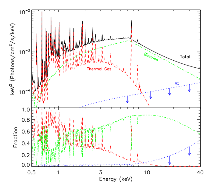
Figure 14.— Unfolded model of the X-ray emission from NGC 253 based on fits to global Chandra and NuSTAR spectra over the 0.5–40 keV energy range (top panel). The fit includes three APEC models representing thermal gas from the disk and starburst-driven winds (“Thermal Gas,” red/dashed line), a broken power law model incorporating all the emission from XRB point sources (“Binaries,” green/dot-dashed line), and a power law model indicating our most conservative upper limit for IC emission as found in Section 4.2.2 (“IC,” blue/dotted line). The fraction of emission attributed to each component is given in the bottom panel. Point source emission prevails above $\sim 1.5$ keV and peaks between 6 and 7 keV, declining at higher energies due to the intermediate-like states of the ULX sources that dominate the NuSTAR spectrum. Diffuse IC emission does not contribute appreciably below 40 keV.

Although the observed luminosity is not a strong function of energy, it peaks in the 2–10 keV band with $L_{X}=7.3\times 10^{39}$ ergs s^-1, compared to the slightly lower luminosities at lower ($L_{X}=4.1\times 10^{39}$ ergs s^-1, 0.5–2 keV) and higher ($L_{X}=2.1\times 10^{39}$ ergs s^-1, 10–40 keV) energies.

6.4. Contribution of Starburst Galaxies to the CXB

The CXB peaks in $\nu F_{\nu}$ at $E\sim 30$ keV (e.g., Gruber et al., 1999) and has yet to be fully resolved into contributing source populations at $E>10$ keV. Focusing hard X-ray telescopes, of which NuSTAR is the first, are expected to make major headway on this issue and it is expected that up to 50% of the hard CXB will ultimately be resolved in NuSTAR deep surveys (Ballantyne et al., 2011). While it is clearly the case that AGN and clusters dominate the overall flux of the CXB at energies below 10 keV (e.g., Worsley et al., 2006), starburst galaxies, given their large numbers and strong evolution with cosmic time (there are many more luminous starburst galaxies at high redshift) could have a non-negligible contribution to the hard CXB. This idea was put forth in Persic & Rephaeli (2003), who took a template X-ray spectrum for starburst galaxies and calculated their contribution to the CXB assuming that their density evolves as $(1+z)^{q}$ up to $z=5$. They found that at energies $E\mathrel{\hbox to0.0pt{\lower 3.0pt\hbox{$\mathchar 536\relax$}\hss}\raise 2.0pt\hbox{$\mathchar 316\relax$}}15$ keV this contribution is at a level of a few percent for $q\leq 3$. Recent deep Chandra surveys have found luminosity evolution consistent with lower values of $q$ ($q=2-3$; e.g., Norman et al., 2004; Ptak et al., 2007; Tzanavaris & Georgantopoulos, 2008; Tremmel et al., 2013). However, Persic & Rephaeli (2003) also predicted that the IC component (see Section 6.2) would be the main contributor to starburst galaxy emission at $E>10$ keV and that its relative contribution would get progressively higher for increasing redshift.

We thus compare the NuSTAR NGC 253 spectrum, which we have modeled extensively in Section 4.1.3, to the model of Persic & Rephaeli (2003) to determine what the possible implications may be for the contribution of starburst galaxies to the CXB. Their model consists of (i) an unabsorbed 0.8 keV thermal bremsstrahlung component from diffuse gas, (ii) an exponentially cutoff power-law representing the XRB populations, with photon index $\Gamma=1.2$ and cutoff energy of 7.5 keV absorbed through $n_{\rm H}$ = $10^{22}$ cm^-2, (iii) a similarly absorbed power-law with photon index $\Gamma_{1}=1.8$ representing the IC emission upscattered from the FIR, and (iv) a very faint unabsorbed power-law with photon index $\Gamma_{2}=2.3$ representing the IC emission upscattered from the cosmic microwave background. The model of Persic & Rephaeli (2003) estimate that the latter two components, (iii) and (iv), respectively account for 5% and 0.5% of the 2-10 keV flux of starburst galaxies, and $\sim 10$% of the flux at 20 keV.

In comparison to the NuSTAR spectrum of NGC 253, we find that the cutoff power-law for the XRB population is too flat. Even with the cut-off, we require a power law slope of $\Gamma>2$. Note that if we lacked the NuSTAR spatial resolution and applied the model of Persic & Rephaeli (2003) to the full NGC 253 hard X-ray spectrum, the contribution of Source 8 may have been interpreted as a (weak) IC component. If the source is an accreting pulsar, we expect the spectrum to turn over quickly above $\sim 20$ keV, so misidentifying it with IC emission would lead to incorrect conclusions for NGC 253’s output at energies above 20 keV. If it is instead a background AGN, then the spectrum of the galaxy would of course be even softer at hard energies. Our constraints on the IC component show that likely $<1$% of the 2–10 keV flux and $<2$% of the 10–30 keV flux, from starburst galaxies arises from IC emission. Importantly, the overall normalization of the 10–30 keV flux is much lower than previously assumed.

Detailed modeling of the type conducted in Persic & Rephaeli (2003) is beyond the scope of this paper. The models shown in their Figure 3, however, allow one to determine resolved fractions based on values for $q$ (see above) and also for the contribution by XRB populations and IC emission. Choosing $q=3$ and neglecting the IC components (iii) and (iv), which we find to be much lower and likely insignificant, we arrive at a starburst galaxy contribution to the $E>10$ keV CXB of $<1$%.

6.5. Variability

6.5.1 X-ray Fluxes

Due to sensitivity limitations, only 8 sources are sufficiently bright to investigate flux variations among epochs. Of these, only Source 7 undergoes a clear state transition. Source 1 varies solely in overall luminosity, Sources 5, 6, and 8 show no significant variations, and the three nuclear sources were addressed in Lehmer et al. (2013). NuSTAR separates the hard emission of these sources – except the nuclear ones – and allows the identification of black hole and neutron star binary states more robustly than is possible otherwise.

Distinguishing one absorbed spectral model from another in lower signal-to-noise data at $E\mathrel{\hbox to0.0pt{\lower 3.0pt\hbox{$\mathchar 536\relax$}\hss}\raise 2.0pt\hbox{$\mathchar 316\relax$}}10$ keV can be challenging, since only at hard energies do degeneracies caused by the effect of absorption vanish. NuSTAR’s collecting area near to and just above 10 keV provides a stronger lever arm to distinguish true MCD components from highly absorbed power law spectra. Although the soft/intermediate states of Sources 5-7 are in general better fit by a pure MCD model, they also exhibit slight hard energy excesses above that model that are even better fit by the addition of a non-thermal component. We cannot place strong constraints at $E>20$ keV to perform fits similar to binaries in the MW (e.g., Steiner et al., 2009; Natalucci et al., 2014). Even so, we are able to rule out simple power law descriptions of the data, confirming much of the emission originates from a disk-like component in these XRBs.

6.5.2 VLBA Flare Monitoring

Among the Galactic XRBs, the ones with the strongest radio emission, Cyg X-3 and SS 433, have high mass donors. Presumably this is because the jets from these systems interact with the winds of the mass donors, leading to more efficient dissipation of energy, and hence a higher radiative efficiency for the jet. Cyg X-3 shows several multi-Jy flares per year (e.g., Waltman et al., 1995), so if the rate of such flares scales with the star formation rate of the host galaxy, we might expect a $\mathrel{\hbox to0.0pt{\lower 3.0pt\hbox{$\mathchar 536\relax$}\hss}\raise 2.0pt\hbox{$\mathchar 318\relax$}}100$ $\mu$Jy flare every few days in NGC 253. The span of our three 8 hr exposures as originally conceived allowed for an excellent chance of catching such a flare. Our probability of detecting a flare was, however, diminished by lower-than-expected sensitivity ($\sim 150$ $\mu$Jy beam^-1) due to telescope failures or missing data, interference, and the low declination of the galaxy. No flares were detected.

There have already been examples of radio/X-ray monitoring, e.g., in M82, that have turned up extremely luminous radio flares. One example is the recent detection of a faint radio source in the nuclear region of M82 using MERLIN by Muxlow et al. (2010). The true nature of this source remains unclear but it may be the first detection of radio emission from an extragalactic microquasar. Recent Chandra analysis by Joseph et al. (2011) shows that the source is not especially bright in X-rays, and hence that it may be an extra-bright SS 433-like object, rather than an extremely radio-bright “normal” microquasar. Radio emission has also been detected from an ULX in M31 (Middleton et al., 2013), albeit at a radio flux well below what could be detected at the distance of the nearest starburst galaxies.

6.6. Future Work

NGC 253 is the benchmark deep observation in a sample of starburst galaxies that have or will have concurrent observations with Chandra and NuSTAR. These galaxies are listed in Harrison et al. (2013) and together provide an in-depth view of XRB populations in the hard X-ray band over a range of stellar masses and star formation rates. This program is critical for understanding the ionizing output of XRB populations and of particular interest is the much deeper view of high-redshift galaxies coming up later in 2014 via the Chandra Deep Field 7 Ms survey (P.I. Niel Brandt), which should detect star-forming galaxies at $z\mathrel{\hbox to0.0pt{\lower 3.0pt\hbox{$\mathchar 536\relax$}\hss}\raise 2.0pt\hbox{$\mathchar 318\relax$}}4$ (Basu-Zych et al., 2013). Note that the observed 2–10 keV Chandra bandpass corresponds to restframe $E=10$–50 keV at $z=4$. Given that XRB populations in starburst galaxies may rival AGN as an ionizing source during the critical reionization period of the Universe (Fragos et al., 2013) – but that the bolometric correction from total starburst luminosity to X-ray bandpass depends sensitively on the spectrum in the hard X-ray bandpass – this NuSTAR program has an important role to play.

We also note that Astro-H will launch late in 2015 and will contain a hard X-ray instrument, the Hard X-ray Imager (HXI), with a bandpass similar to that of NuSTAR. The HXI has a slightly larger PSF than NuSTAR at $\sim 1.8$^′; however, the background is anticipated to be slightly lower and the collecting area higher, so the overall sensitivity should be comparable for overall detection of NGC 253 and other starburst galaxies. We expect that multiple observations from both Astro-H and NuSTAR, collected over the years, will provide highly valuable constraints on accretion state transitions of the bright X-ray binary population in NGC 253. The accumulated broad-band spectrum from these observations would substantially improve measurements of the $E>30$ keV emission and the corresponding contribution from IC emission.

References

- Abdo et al. (2010) Abdo, A. A., Ackermann, M., Ajello, M., et al. 2010, ApJ, 709, L152
- Abramowski et al. (2012) Abramowski, A., Acero, F., Aharonian, F., et al. 2012, ApJ, 757, 158
- VERITAS Collaboration et al. (2009) VERITAS Collaboration, Acciari, V. A., Aliu, E., et al. 2009, Nature, 462, 770
- Acero et al. (2009) Acero, F., Aharonian, F., Akhperjanian, A. G., et al. 2009, Science, 326, 1080
- Ackermann et al. (2012) Ackermann, M., Ajello, M., Allafort, A., et al. 2012, ApJ, 755, 164
- Argo et al. (in prep.) Argo et al. 2014, in prep.
- Bachetti et al. (2013) Bachetti, M., Rana, V., Walton, D. J., et al. 2013, ApJ, 778, 163
- Ballantyne et al. (2011) Ballantyne, D. R., Draper, A. R., Madsen, K. K., Rigby, J. R., & Treister, E. 2011, ApJ, 736, 56
- Basu-Zych et al. (2013) Basu-Zych, A. R., Lehmer, B. D., Hornschemeier, A. E., et al. 2013, ApJ, 774, 152
- Bauer & Pietsch (2005) Bauer, M., & Pietsch, W. 2005, A&A, 442, 925
- Bauer et al. (2007) Bauer, M., Pietsch, W., Trinchieri, G., et al. 2007, A&A, 467, 979
- Bauer et al. (2008) Bauer, M., Pietsch, W., Trinchieri, G., et al. 2008, A&A, 489, 1029
- Bookbinder et al. (1980) Bookbinder, J., Cowie, L. L., Ostriker, J. P., Krolik, J. H., & Rees, M. 1980, ApJ, 237, 647
- Booth et al. (2013) Booth, C. M., Agertz, O., Kravtsov, A. V., & Gnedin, N. Y. 2013, ApJ, 777, L16
- Brunthaler et al. (2009) Brunthaler, A., Castangia, P., Tarchi, A., et al. 2009, A&A, 497, 103
- Cappi et al. (1999) Cappi, M., Persic, M., Bassani, L., et al. 1999, A&A, 350, 777
- Cash (1979) Cash, W. 1979, ApJ, 228, 939
- Chakraborty & Fields (2013) Chakraborty, N., & Fields, B. D. 2013, ApJ, 773, 104
- Dahlem et al. (1998) Dahlem, M., Weaver, K. A., & Heckman, T. M. 1998, ApJS, 118, 401
- Deller et al. (2011) Deller, A. T., Brisken, W. F., Phillips, C. J., et al. 2011, PASP, 123, 275
- Domingo-Santamaría & Torres (2005) Domingo-Santamaría, E., & Torres, D. F. 2005, A&A, 444, 403
- Done et al. (2007) Done, C., Gierliński, M., & Kubota, A. 2007, A&A Rev., 15, 1
- Dunn et al. (2010) Dunn, R. J. H., Fender, R. P., Körding, E. G., Belloni, T., & Cabanac, C. 2010, MNRAS, 403, 61
- Fabbiano & Trinchieri (1984) Fabbiano, G., & Trinchieri, G. 1984, ApJ, 286, 491
- Fender et al. (2004) Fender, R. P., Belloni, T. M., & Gallo, E. 2004, MNRAS, 355, 1105
- Fragos et al. (2013) Fragos, T., Lehmer, B. D., Naoz, S., Zezas, A., & Basu-Zych, A. 2013, ApJ, 776, L31
- Gendre et al. (2013) Gendre, M. A., Fenech, D. M., Beswick, R. J., Muxlow, T. W. B., & Argo, M. K. 2013, MNRAS, 431, 1107
- Gregory et al. (1972) Gregory, P. C., Kronberg, P. P., Seaquist, E. R., et al. 1972, Nature Physical Science, 239, 114
- Gruber et al. (1999) Gruber, D. E., Matteson, J. L., Peterson, L. E., & Jung, G. V. 1999, ApJ, 520, 124
- Harrison et al. (2013) Harrison, F. A., Craig, W. W., Christensen, F. E., et al. 2013, ApJ, 770, 103
- Hornschemeier et al. (2003) Hornschemeier, A. E., Bauer, F. E., Alexander, D. M., et al. 2003, AJ, 126, 575
- Joseph et al. (2011) Joseph, T. D., Maccarone, T. J., & Fender, R. P. 2011, MNRAS, 415, L59
- Jubelgas et al. (2008) Jubelgas, M., Springel, V., Enßlin, T., & Pfrommer, C. 2008, A&A, 481, 33
- Kajava & Poutanen (2009) Kajava, J. J. E., & Poutanen, J. 2009, MNRAS, 398, 1450
- Karachentsev et al. (2003) Karachentsev, I. D., Grebel, E. K., Sharina, M. E., et al. 2003, A&A, 404, 93
- Kelner et al. (2006) Kelner, S. R., Aharonian, F. A., & Bugayov, V. V. 2006, Phys. Rev. D, 74, 034018
- Koljonen et al. (2010) Koljonen, K. I. I., Hannikainen, D. C., McCollough, M. L., Pooley, G. G., & Trushkin, S. A. 2010, MNRAS, 406, 307
- Kyanidis & Zezas (in prep.) Kyanidis, S., & Zezas, A. 2014, in prep.
- Lacki et al. (2012) Lacki, B. C., Horiuchi, S., & Beacom, J. F. 2012, arXiv:1206.0772
- Lacki & Thompson (2013) Lacki, B. C., & Thompson, T. A. 2013, ApJ, 762, 29
- Lehmer et al. (2010) Lehmer, B. D., Alexander, D. M., Bauer, F. E., et al. 2010, ApJ, 724, 559
- Lehmer et al. (2012) Lehmer, B. D., Xue, Y. Q., Brandt, W. N., et al. 2012, ApJ, 752, 46
- Lehmer et al. (2013) Lehmer, B. D., Wik, D. R., Hornschemeier, A. E., et al. 2013, ApJ, 771, 134
- Lenc & Tingay (2006) Lenc, E., & Tingay, S. J. 2006, AJ, 132, 1333
- Longair (1994) Longair, M. S. 1994, Cambridge: Cambridge University Press, 2nd ed.
- Liu & Bregman (2005) Liu, J.-F., & Bregman, J. N. 2005, ApJS, 157, 59
- Maccarone (2003) Maccarone, T. J. 2003, A&A, 409, 697
- Maccarone & Coppi (2003) Maccarone, T. J., & Coppi, P. S. 2003, MNRAS, 338, 189
- Maccarone et al. (2014) Maccarone, T. J., Lehmer, B. D., Leyder, J. C., et al. 2014, MNRAS, 339
- Makishima et al. (1986) Makishima, K., Maejima, Y., Mitsuda, K., et al. 1986, ApJ, 308, 635
- McCollough et al. (2010) McCollough, M. L., Koljonen, K. I. I., & Hannikainen, D. C. 2010, arXiv:1003.4278
- McDonald et al. (2002) McDonald, A. R., Muxlow, T. W. B., Wills, K. A., Pedlar, A., & Beswick, R. J. 2002, MNRAS, 334, 912
- Mesinger et al. (2013) Mesinger, A., Ferrara, A., & Spiegel, D. S. 2013, MNRAS, 431, 621
- Middleton et al. (2013) Middleton, M. J., Miller-Jones, J. C. A., Markoff, S., et al. 2013, Nature, 493, 187
- Mioduszewski et al. (2001) Mioduszewski, A. J., Rupen, M. P., Hjellming, R. M., Pooley, G. G., & Waltman, E. B. 2001, ApJ, 553, 766
- Mitsuishi et al. (2011) Mitsuishi, I., Yamasaki, N. Y., & Takei, Y. 2011, ApJ, 742, L31
- Mitsuishi et al. (2013) Mitsuishi, I., Yamasaki, N. Y., & Takei, Y. 2013, PASJ, 65, 44
- Miyasaka et al. (2013) Miyasaka, H., Bachetti, M., Harrison, F. A., et al. 2013, ApJ, 775, 65
- Müller-Sánchez et al. (2010) Müller-Sánchez, F., González-Martín, O., Fernández-Ontiveros, J. A., Acosta-Pulido, J. A., & Prieto, M. A. 2010, ApJ, 716, 1166
- Muxlow et al. (2010) Muxlow, T. W. B., Beswick, R. J., Garrington, S. T., et al. 2010, MNRAS, 404, L109
- Natalucci et al. (2014) Natalucci, L., Tomsick, J. A., Bazzano, A., et al. 2014, ApJ, 780, 63
- Norman et al. (2004) Norman, C., Ptak, A., Hornschemeier, A., et al. 2004, ApJ, 607, 721
- Oosterbroek et al. (1998) Oosterbroek, T., Parmar, A. N., Kuulkers, E., et al. 1998, A&A, 340, 431
- Pacucci et al. (2014) Pacucci, F., Mesinger, A., Mineo, S., & Ferrara, A. 2014, arXiv:1403.6125
- Paglione & Abrahams (2012) Paglione, T. A. D., & Abrahams, R. D. 2012, ApJ, 755, 106
- Pence (1980) Pence, W. D. 1980, ApJ, 239, 54
- Persic et al. (1998) Persic, M., Mariani, S., Cappi, M., et al. 1998, A&A, 339, L33
- Persic & Rephaeli (2002) Persic, M., & Rephaeli, Y. 2002, A&A, 382, 843
- Persic & Rephaeli (2003) Persic, M., & Rephaeli, Y. 2003, A&A, 399, 9
- Pietsch et al. (2000) Pietsch, W., Vogler, A., Klein, U., & Zinnecker, H. 2000, A&A, 360, 24
- Pietsch et al. (2001) Pietsch, W., Roberts, T. P., Sako, M., et al. 2001, A&A, 365, L174
- Portegies Zwart et al. (2004) Portegies Zwart, S. F., Dewi, J., & Maccarone, T. 2004, MNRAS, 355, 413
- Predehl et al. (2000) Predehl, P., Burwitz, V., Paerels, F., & Trümper, J. 2000, A&A, 357, L25
- Press et al. (2002) Press, W. H., Teukolsky, S. A., Vetterling, W. T., & Flannery, B. P. 2002, Numerical recipes in C++ : the art of scientific computing by William H. Press. xxviii, 1,002 p. : ill. ; 26 cm. Includes bibliographical references and index. ISBN : 0521750334,
- Ptak et al. (1997) Ptak, A., Serlemitsos, P., Yaqoob, T., Mushotzky, R., & Tsuru, T. 1997, AJ, 113, 1286
- Ptak et al. (2007) Ptak, A., Mobasher, B., Hornschemeier, A., Bauer, F., & Norman, C. 2007, ApJ, 667, 826
- Ptak et al. (2014) Ptak, A., Hornschemeier, A., Zezas, A., et al. 2014, ApJ, submitted
- Puche & Carignan (1988) Puche, D., & Carignan, C. 1988, AJ, 95, 1025
- Rampadarath et al. (2014) Rampadarath, H., Morgan, J. S., Lenc, E., & Tingay, S. J. 2014, AJ, 147, 5
- Rana et al. (2014) Rana, V., Harrison, F. A., Bachetti, M., et al. 2014, arXiv:1401.4637
- Read et al. (1997) Read, A. M., Ponman, T. J., & Strickland, D. K. 1997, MNRAS, 286, 626
- Reig et al. (2003) Reig, P., Belloni, T., & van der Klis, M. 2003, A&A, 412, 229
- Reig (2011) Reig, P. 2011, Ap&SS, 332, 1
- Rephaeli et al. (1995) Rephaeli, Y., Gruber, D., & Persic, M. 1995, A&A, 300, 91
- Rephaeli et al. (2010) Rephaeli, Y., Arieli, Y., & Persic, M. 2010, MNRAS, 401, 473
- Remillard & McClintock (2006) Remillard, R. A., & McClintock, J. E. 2006, ARA&A, 44, 49
- Salem & Bryan (2013) Salem, M., & Bryan, G. L. 2013, arXiv:1307.6215
- Schober et al. (2014) Schober, J., Schleicher, D. R. G., & Klessen, R. S. 2014, arXiv:1404.2578
- Siebenmorgen & Krügel (2007) Siebenmorgen, R., & Krügel, E. 2007, A&A, 461, 445
- Socrates et al. (2008) Socrates, A., Davis, S. W., & Ramirez-Ruiz, E. 2008, ApJ, 687, 202
- Stark et al. (1992) Stark, A. A., Gammie, C. F., Wilson, R. W., et al. 1992, ApJS, 79, 77
- Steiner et al. (2009) Steiner, J. F., Narayan, R., McClintock, J. E., & Ebisawa, K. 2009, PASP, 121, 1279
- Strickland et al. (2000) Strickland, D. K., Heckman, T. M., Weaver, K. A., & Dahlem, M. 2000, AJ, 120, 2965
- Strickland et al. (2004) Strickland, D. K., Heckman, T. M., Colbert, E. J. M., Hoopes, C. G., & Weaver, K. A. 2004, ApJS, 151, 193
- Strong et al. (2010) Strong, A. W., Porter, T. A., Digel, S. W., et al. 2010, ApJ, 722, L58
- Tananbaum et al. (1972) Tananbaum, H., Gursky, H., Kellogg, E., Giacconi, R., & Jones, C. 1972, ApJ, 177, L5
- Tingay (2004) Tingay, S. J. 2004, AJ, 127, 10
- Torres et al. (2004) Torres, D. F., Reimer, O., Domingo-Santamaría, E., & Digel, S. W. 2004, ApJ, 607, L99
- Tremmel et al. (2013) Tremmel, M., Fragos, T., Lehmer, B. D., et al. 2013, ApJ, 766, 19
- Tzanavaris & Georgantopoulos (2008) Tzanavaris, P., & Georgantopoulos, I. 2008, A&A, 480, 663
- Uhlig et al. (2012) Uhlig, M., Pfrommer, C., Sharma, M., et al. 2012, MNRAS, 423, 2374
- Vadawale et al. (2003) Vadawale, S. V., Rao, A. R., Naik, S., et al. 2003, ApJ, 597, 1023
- van Haaften et al. (2012) van Haaften, L. M., Voss, R., & Nelemans, G. 2012, A&A, 543, A121
- Vogler & Pietsch (1999) Vogler, A., & Pietsch, W. 1999, A&A, 342, 101
- Waltman et al. (1995) Waltman, E. B., Ghigo, F. D., Johnston, K. J., et al. 1995, AJ, 110, 290
- Walton et al. (2013) Walton, D. J., Fuerst, F., Harrison, F., et al. 2013, ApJ, 779, 148
- Walton et al. (2014) Walton, D. J., Harrison, F. A., Grefenstette, B. W., et al. 2014, arXiv:1402.2992
- Weaver et al. (2002) Weaver, K. A., Heckman, T. M., Strickland, D. K., & Dahlem, M. 2002, ApJ, 576, L19
- Wik el al. (2014) Wik, D., Hornstrup, A., Molendi, S., et al. 2014, ApJ, 792, 48
- Winter et al. (2009) Winter, L. M., Mushotzky, R. F., Reynolds, C. S., & Tueller, J. 2009, ApJ, 690, 1322
- Worsley et al. (2006) Worsley, M. A., Fabian, A. C., Bauer, F. E., et al. 2006, MNRAS, 368, 1735