Enhancement of the thermal expansion of organic charge transfer salts
by strong electronic correlations

Abstract

Organic charge transfer salts exhibit thermal expansion anomalies similar to those found in other strongly correlated electron systems. The thermal expansion can be anisotropic and have a non-monotonic temperature dependence. We show how these anomalies can arise from electronic effects and be significantly enhanced, particularly at temperatures below 100 K, by strong electronic correlations. For the relevant Hubbard model the thermal expansion is related to the dependence of the entropy on the parameters ($t$, $t^{\prime}$, and $U$) in the Hamiltonian or the temperature dependence of bond orders and double occupancy. The latter are calculated on finite lattices with the Finite Temperature Lanczos Method. Although many features seen in experimental data, in both the metallic and Mott insulating phase, are described qualitatively, the calculated magnitude of the thermal expansion is smaller than that observed experimentally.

I Introduction

The thermal expansion coefficients of a wide range of strongly correlated electron materials exhibit temperature and orientational dependencies that are distinctly different from simple metals and insulatorsWhite (1993). Materials that have been studied included heavy fermion compounds Lacerda et al. (1989), organic charge transfer salts Müller et al. (2002); de Souza et al. (2007); Manna et al. (2010); de Souza and Pouget (2013), iron pnictide superconductors Meingast et al. (2012); Hardy et al. (2013), and LiV₂O₄ Johnston et al. (1999). The Grüneisen parameter $\Gamma$, which is proportional to the ratio of the thermal expansion to the specific heat, can be two orders of magnitude larger than the values of order unity found for elemental solids Lacerda et al. (1989), and may diverge at a quantum critical point Zhu et al. (2003). For organic charge transfer salts, the thermal expansion coefficients show anomalies at the superconducting transition temperature Müller et al. (2000), at the Fermi liquid coherence temperature, at the Mott transition, and strong non-monotonic temperature and orientational dependence Müller et al. (2002). Anomalies have been recently observed also in a spin liquid candidate material, $\kappa$-(BEDT-TTF)₂Cu₂(CN)₃ Manna et al. (2010). For a proper understanding and interpretation of these experimental results it is important to elucidate the electronic (apart from the phononic) contribution to the thermal expansion, particularly since it may dominate at low temperatures. Related electronic effects are seen in lattice softening near the Mott transition via sound velocity measurements Fournier et al. (2003); Hassan et al. (2005). The electronic contribution can also lead to the critical behaviour of the thermal expansion close to the metal-insulator transition de Souza et al. (2007); Zacharias et al. (2012).

Here we study the electronic contribution to the thermal expansion, including its directional dependence, by modelling the electrons with a Hubbard model on the anisotropic triangular lattice at half filling, an effective model Hamiltonian for several families of organic charge transfer salts Powell and McKenzie (2011). Our analysis requires a connection between the Hubbard model parameters ($t$, $t^{\prime}$, $U$) and structural parameters (lattice constants) that can be deduced from electronic structure calculations and bulk compressibilities for which we use experimental values.

I.1 Summary of results

Our main results concerning the electronic contribution to the thermal expansion $\alpha$ are as follows.

(i) At low temperatures strong correlations can increase the thermal expansion by as much as an order of magnitude.

(ii) A non-monotonic temperature dependence of $\alpha$ is possible.

(iii) Significant orientational dependence is possible, including the expansion having the opposite sign in different directions.

(iv) In the metallic phase the crossover from a Fermi liquid to a bad metal may be reflected in a maximum in the temperature dependence of $\alpha$.

(v) In the Mott insulating phase a maximum in the temperature dependence of $\alpha$ can occur, at a temperature comparable to that at which a maximum also occurs in the specific heat and the magnetic susceptibility.

(vi) All of the above results are sensitive to the proximity to the Mott metal-insulator transition and the amount of frustration, reflected in the parameter values ($U/t$ and $t^{\prime}/t$) in the Hubbard model.

Although, we can describe many of the unusual qualitative features of experimental data for organic charge transfer salts, the overall magnitude of the thermal expansion coefficients that we calculate are up to an order of magnitude smaller than observed. This disagreement may arise from uncertainties in how uniaxial stress changes the Hubbard model parameters, and uncertainty in the compressibilities including not taking into account the effect of softening of the lattice associated with proximity to the Mott transition.

I.2 Specific experimental results we focus on

We briefly review some experimental results that our calculations are directly relevant to. We only consider thermal expansion within the conducting layers. Anomalies are also seen in the interlayer direction but are beyond the scope of this study. Figure 1 shows the relation between the anisotropic triangular lattice, and the associated hoppings $t$ and $t^{\prime}$, and the intralayer crystal axes ($b$ and $c$) for $\kappa$ -(BEDT-TTF)₂X with anions X=Cu₂(CN)₃ and Cu(NCS)₂. For X= Cu[N(CN)₂]Br, the crystal axes $b$ and $c$ should be replaced with $c$ and $a$, respectively.

Figure 1: Lattice and hopping integrals in the Hubbard model for $\kappa$ -(BEDT-TTF)₂X with X=Cu₂(CN)₃ and Cu(NCS)₂. For X= Cu[N(CN)₂]Br the crystal axes $b$ and $c$ should be replaced with $c$ and $a$.

Mott insulating phase of $\kappa$-(BEDT-TTF)₂Cu₂(CN)₃ [Figure 1 in Ref. Manna et al., 2010]. For some temperature ranges thermal expansion in the $b$ ($t^{\prime}$) and $c$ ($t$) directions have opposite signs. Thermal expansion is a non-monotonic function of temperature. $\alpha_{b}$ and $\alpha_{c}$ have extremal values at about 60 K and 30 K, respectively. For comparison, the magnetic susceptibility has a maximum at a temperature around 60 K Shimizu et al. (2003).

Metallic phase of un-deuterated $\kappa$-(BEDT-TTF)₂Cu[N(CN)₂]Br [Figure 5a in Ref. Müller et al., 2002]. As the temperature decreases there is a crossover from a bad metal to a Fermi liquid.Merino et al. (2008) $\alpha_{a}$ is a non-monotonic function of temperature, with a large maximum around 35 K, which is comparable to the temperature at which there is a large change in slope of the resistivity versus temperature curve Yu et al. (1991). This is one measure of the coherence temperature associated with the crossover from the bad metal to the Fermi liquid.Deng et al. (2013)

Mott transition in fully deuterated $\kappa$-(BEDT-TTF)₂Cu[N(CN)₂]Br [Figure 1 in Ref. de Souza et al., 2007 and Figure 2 in Ref. Lang et al., 2008]. As the temperature decreases there is a crossover from a bad metal to a Fermi liquid to a Mott insulator (below 14 K). $\alpha_{c}$ (direction of $t^{\prime}$) is much smaller than $\alpha_{a}$ (direction of $t$) and monotonically increases with temperature. In contrast, $\alpha_{a}$ is a non-monotonic function of temperature, with a large maximum around 30 K, which is comparable to the temperature at which the crossover from the bad metal to the Fermi liquid occurs. Also, $\alpha_{a}$ is negative in the Mott insulating phase.

I.3 Outline

The outline of the paper is as follows. In Section II we discuss how the thermal expansion is related to variations in the entropy through Maxwell relations from thermodynamics. In Section III the relevant Hubbard model is introduced and it is shown how the temperature dependence of bond orders is related to the thermal expansion. We also discuss how the parameters in the Hubbard model depend on the lattice constants. Results of calculations of the bond orders using the Finite Temperature Lanczos Method are presented in Section IV. Comparisons are made between the calculated thermal expansion (for a range of parameter values) and specific experiments on organic charge transfer salts. This is followed by discussion of remaining future challenges, while we summarize our main conclusions in Section V.

II General thermodynamic considerations

For simplicity and to elucidate the essential physics we first discuss the isotropic case. Experiments are done at constant temperature, pressure, and particle number (assuming the sample is not connected to electrical leads and the particle density is controlled by chemistry). Thus, the Gibbs free energy $G(T,P,N_{e})$ is a minimum and satisfies

$$dG=-SdT+VdP+\mu dN_{e}.$$ (1)

From this we can derive a Maxwell relation implying that the volume thermal expansion is given by

$$\alpha(T)\equiv{1\over V}\left({\partial V\over\partial T}\right)_{P}=-{1\over V}\left({\partial S\over\partial P}\right)_{T}.$$ (2)

In calculations it is however easier to vary the volume than pressure and so we rewrite this as

$$\alpha(T)=-{1\over V}\left({\partial V\over\partial P}\right)_{T}\left({\partial S\over\partial V}\right)_{T}=\kappa_{T}\left({\partial S\over\partial V}\right)_{T},$$ (3)

where $\kappa_{T}$ is the isothermal bulk compressibility. Given the expression above it is natural to expect strong thermal expansion effects when the entropy is large (e.g., at the incoherence crossover) and sensitive to volume-dependent parameters in the system (e.g., close to the Mott transition).

As the volume changes so do the lattice constants and the parameters in an underlying electronic Hamiltonian such as the hopping integral $t$ in a Hubbard model. To evaluate (3) we use

$$\left({\partial S\over\partial V}\right)_{T,N_{e}}={\partial t\over\partial V}\left({\partial S\over\partial t}\right)_{T,N_{e}},$$ (4)

leading to

$$\alpha(T)=\kappa_{T}{\partial t\over\partial V}\left({\partial S\over\partial t}\right)_{T,N_{e}}.$$ (5)

This equation for volume thermal expansion applies for isotropic case, while orientational dependance of thermal expansion can be obtained in a similar manner by generalizing $VdP$ to $-\sum_{i}d\sigma_{i}V^{0}l_{i}/l_{i}^{0}$. Here $i=x,y,z$, $d\sigma_{i}$ is the change of uniaxial stress, $l_{i}$ is the length in $i$ direction, while $V^{0}$ and $l_{i}^{0}$ are reference volume and length. Thermal expansion in direction $i$ is then, similarly as Eq. 4, given by

$$\alpha_{i}(T)=\frac{1}{E_{i}}\frac{l_{i}^{0}}{V^{0}}{\partial t\over\partial l_{i}}\left({\partial S\over\partial t}\right)_{T,N_{e}}+\cdots$$ (6)

Additional terms involve different electronic model parameters instead of $t$, e.g., $t^{\prime}$ and $U$. This expression is valid for small Poisson’s ratio, which is together with more detailed derivation in terms of the grand potential ($\Omega=G-PV-\mu N_{e}$) discussed in Appendix A. The value of the Young’s modulus $E_{i}$ we take from experiment and later comment on the effect of the Mott transition on it. We estimate $\partial t/\partial l_{i}$ from band structure calculations and we calculate $\partial S/\partial t$ numerically with the Finite Temperature Lanczos Method (FTLM) Jaklič and Prelovšek (2000); Kokalj and McKenzie (2013). It follows from the third law of thermodynamics that $\alpha_{i}(T)\to 0$ as $T\to 0$.

III Hubbard model

We model our system with two Hamiltonian terms, $\hat{H}=\hat{H}_{el}+\hat{H}_{other}$, where $\hat{H}_{el}$ describes electrons in the highest occupied band and their contribution to the thermal expansion is our main interest. We decouple these electronic degrees of freedom from others such as phonons and electrons in lower filled bands, and denote their contribution with $\hat{H}_{other}$. With this we neglected the direct coupling of electrons and phonons, but we keep the dependence of $\hat{H}_{el}$ on the lattice constants $a_{i}$, which is in the spirit of a Born-Oppenheimer approximation.

We model the electrons in the highest occupied band with the grand canonical Hubbard model on the anisotropic triangular lattice,

$$\hat{H}_{el} = -\sum_{i,j,\sigma}t_{i,j}c_{i,\sigma}^{\dagger}c_{j,\sigma}+U\sum_{i}\hat{n}_{i,\uparrow}\hat{n}_{i,\downarrow}-\mu\sum_{i,\sigma}\hat{n}_{i,\sigma}$$ (7)

$$= -t\hat{T}_{1}-t^{\prime}\hat{T}_{2}+U\hat{D}-\mu\hat{N}_{e}.$$

Here $t_{i,j}=t$ for nearest neighbor bonds in two directions and $t_{i,j}=t^{\prime}$ for nearest neighbor bonds in the third direction (compare Figure 1). Electronic spin is denoted with $\sigma$ ($\uparrow$ or $\downarrow$). $\hat{T}_{1}$ and $\hat{T}_{2}$ denote bond order operators corresponding to $t$ and $t^{\prime}$ hopping respectively, and $\hat{D}$ is the double occupancy operator. The chemical potential $\mu(T)$ is determined by the required half filling, i.e. that $\langle\hat{N}_{e}\rangle=N_{e}=N$, where $N$ is the number of lattice sites. $\langle\ldots\rangle$ denotes thermal average.

Following equation (6), we relate the thermal expansion to $\left({\partial S\over\partial x}\right)_{T,N_{e}}$ where $x=t,t^{\prime},U$. Using the Maxwell-type relations we can write

$$\left({\partial S\over\partial t}\right)_{T,N_{e},t^{\prime},U}=\left({\partial\langle\hat{T}_{1}\rangle\over\partial T}\right)_{N_{e},t,t^{\prime},U},$$ (8)

$$\left({\partial S\over\partial t^{\prime}}\right)_{T,N_{e},t,U}=\left({\partial\langle\hat{T}_{2}\rangle\over\partial T}\right)_{N_{e},t,t^{\prime},U},$$ (9)

$$\left({\partial S\over\partial U}\right)_{T,N_{e},t,t^{\prime}}=-\left({\partial\langle\hat{D}\rangle\over\partial T}\right)_{N_{e},t,t^{\prime},U}.$$ (10)

With the equations above we related the thermal expansion to the variation of entropy with electronic model parameters ($t,t^{\prime}$ and $U$) or analogously to the $T$ dependence of bond orders ($\langle\hat{T}_{1}\rangle$, $\langle\hat{T}_{2}\rangle$) or double occupancy ($\langle\hat{D}\rangle$), again at fixed particle number.

III.1 Dependence of the Hubbard model parameters on the lattice constants

The expression (6) for the thermal expansion requires knowledge of the dependence of Hubbard model parameters ($t$, $t^{\prime}$ and $U$) on the lattice constants. Estimates of this dependence can be obtained from electronic structure calculations via methods such as extended Hückel or Density Functional Theory (DFT). Calculations using the former with the experimental crystal structure for X=Cu₂(CN)₃ give the following (compare Fig. 8 in Ref. Shimizu et al., 2011),

$$t=t_{0}(1-4.9(\frac{c-c_{0}}{c_{0}})),$$ (11)

$$t^{\prime}=t^{\prime}_{0}(1-8.7(\frac{b-b_{0}}{b_{0}})).$$ (12)

$$U=U_{0}(1-3.5(\frac{b-b_{0}}{b_{0}})-2.8(\frac{c-c_{0}}{c_{0}})).$$ (13)

Here $c$ and $b$ are in-plane lattice constants (compare Figure 1), while reference values at 1 bar pressure are denoted with $c_{0},b_{0},t_{0}$, $t^{\prime}_{0}$ and $U_{0}$. In general the Hubbard model parameters depend on all lattice constants and structural parameters (including angles) Mori (1998); Mori et al. (1999); Kondo et al. (2003); Kandpal et al. (2009); Jeschke et al. (2012) and all should be considered, but for simplicity we keep only the dependencies given above. They were obtainedShimizu et al. (2011) by assuming that squeezing only reduces the intermolecular distance along the direction of the uniaxial stress, but does not induce rotations of molecules.

The actual dependence of the Hubbard $U$ on the structure is subtle. In a crystal such as sodium or nickel oxide $U$ would simply be associated with a single atomic orbital and would not vary with lattice constant and stress, provided screening is neglected. Screening could introduce some dependence. However, for (BEDT-TTF)₂X crystals things are more complicated because $U$ is with respect to a molecular orbital on a dimer of BEDT-TTF molecules and the dimer geometry will vary with uniaxial stress. Furthermore, the estimate given in the expression (13) is based on the assumption that $U$ is solely given by the intradimer hopping integral $2t_{b1}$. However, that is only in the limit $t_{b1}\ll\tilde{U}_{0}$, where $\tilde{U}_{0}$ is the Coulomb repulsion associated with single BEDT-TTF molecule. Although, this assumption is actually unrealistic Powell and McKenzie (2011), Eq. (13) is useful as an estimate, particularly because it is an upper bound for the dependence. Furthermore, we will see below that the $U$ dependence of the entropy is much smaller than that of the $t$ and $t^{\prime}$ dependence (compare Figs. 3 and 4) and so turns out to make a relatively insignificant contribution to the thermal expansion. Hence, the above concerns are not particularly important.

The thermal expansion in the direction of the $c$ axis can therefore be calculated from Eqs. (6), (8), and (11), related to the bond order $\langle\hat{T}_{1}\rangle$, to give

$$\alpha_{c}=\frac{1}{E_{c}}\frac{c_{0}}{NV_{1uc}}\frac{\partial t}{\partial c}\frac{\partial\langle\hat{T}_{1}\rangle}{\partial T}$$ (14)

where $E_{c}$ is the Young’s modulus in the $c$ direction, and we have neglected the contribution from the double occupancy. $V_{1uc}$ denotes the volume of one unit cell. In a similar way, the main contribution to $\alpha_{b}$ is given by the $t^{\prime}$ dependence on $b$ according to Eq. (12) and the temperature derivative of $\langle\hat{T}_{2}\rangle$,

$$\alpha_{b}=\frac{1}{E_{b}}\frac{b_{0}}{NV_{1uc}}\frac{\partial t^{\prime}}{\partial b}\frac{\partial\langle\hat{T}_{2}\rangle}{\partial T}.$$ (15)

These are the expressions we use below to calculate the thermal expansion.

IV Results

In the following we discuss several numerical results obtained on $N=16$ sites by the finite-temperature Lanczos method (FLTM) Jaklič and Prelovšek (2000), which was previously successfully used to determine a range of thermodynamic quantities for the same Hubbard model Kokalj and McKenzie (2013). In particular, it was shown that one could describe the Mott metal-insulator transition and the crossover from a Fermi liquid to a bad metal.

IV.1 Dependence of the entropy on Hubbard model parameters

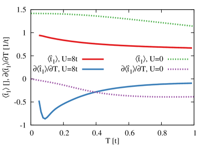
Figure 2: (color online) Strong correlations significantly enhance the electronic contribution to the thermal expansion through the temperature dependence of the bond order. This is demonstrated by comparing $\partial\langle\hat{t}_{1}\rangle/\partial T$ at low $T$ for $U=8t$ with the noninteracting $U=0$ result. $\langle\hat{t}_{1}\rangle=\langle\hat{T}_{1}\rangle/N$ is the average kinetic energy in certain directions. At low temperatures the enhancement is by an order of magnitude. The plotted quantity is related to the thermal expansion via Eq. (14) and to the stress dependence of entropy $s=S/N$ via a Maxwell relation $\partial\langle\hat{t}_{1}\rangle/\partial T=\partial s/\partial t$, Eq. (8). In addition, strong correlations also produce a strong non-monotonic temperature dependence. Results are for $t^{\prime}=0.8t$ and $U=8t$, corresponding to the system in the Mott insulating phase.Kokalj and McKenzie (2013)

In Fig. 2 we show the $T$-derivative of $\langle\hat{t}_{1}\rangle=\langle\hat{T}_{1}\rangle/N$, namely $(1/N)(\partial\langle\hat{T}_{1}\rangle/\partial T)_{t,t^{\prime},U,N_{e}}$, in the insulating phase ($U=8t$, $t^{\prime}=0.8t$ Kokalj and McKenzie (2013)) and compare it to the result for noninteracting fermions ($U=0$). The strong difference shows that correlations can increase the electronic contribution to the thermal expansion by as much as an order of magnitude at low temperatures, and produce a non-monotonic temperature dependence.

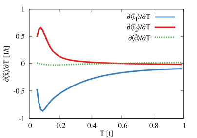
Figure 3: (color online) Strongly anisotropic temperature dependence of the bond orders $\langle\hat{T}_{1}\rangle$ and $\langle\hat{T}_{2}\rangle$. Due to strong correlations and frustration a small anisotropy (i.e. deviation from the isotropy of the triangular lattice) with $t^{\prime}=0.8t$ leads to strongly anisotropic electronic contributions to the thermal expansion. This is seen by comparing $\partial\langle\hat{t}_{1}\rangle/\partial T=\partial s/\partial t$ and $\partial\langle\hat{t}_{2}\rangle/\partial T=\partial s/\partial t^{\prime}$, which are large and have opposite sign at low $T$. For the isotropic case ($t^{\prime}=t$) they have essentially the same $T$ dependence, with only a factor of two difference coming from a number of bonds associated with corresponding hopping. The double occupancy $\langle\hat{d}\rangle=\langle\hat{D}\rangle/N$ shows a much weaker $T$ dependence. Results are for the insulating phase with $t^{\prime}=0.8t$ and $U=8t$ Kokalj and McKenzie (2013).

In Fig. 3 we show that an anisotropy value of $t^{\prime}/t=\leavevmode\nobreak\ 0.8$ leads to strong anisotropy of bond orders and their $T$-derivative relevant for thermal expansion. This probably originates in strong frustration for the isotropic case with large low $T$ entropy and therefore small changes in the anisotropy can lead to strong change of bond orders which in the insulating phase are associated with spin correlations. In Fig. 3 we also show the $T$-derivative of double occupancy which has smaller values than for bond orders. By the Maxwell relation in Eq. (10), our results in Fig. 3 are qualitatively consistent with the $U$ variation of $S$ shown in Fig. 4 of Ref. Kokalj and McKenzie, 2013. This relation of the entropy and negative values of $(\partial\langle\hat{D}\rangle/\partial T)_{t,t^{\prime},N_{e}}$ at low $T$ were recently evoked Li et al. (2014); Laubach et al. (2014) as a possible mechanism for adiabatic cooling in optical lattices.

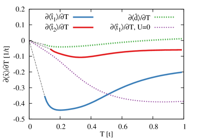
Figure 4: (color online) In the metallic phase ($t^{\prime}=0.8t$, $U=6t$ Kokalj and McKenzie (2013)) the temperature dependence of the bond orders is strongly anisotropic and non-monotonic. At low temperatures, a linear dependence is expected for a Fermi liquid, extrapolating to zero, in accordance with the third law of thermodynamics. This is shown by the dashed lines. The linearity ceases above the coherence temperature $T_{\textrm{coh}}$, where there is a crossover to a bad metal and where a maximum magnitude of the thermal expansion is observed. At low temperatures ($T\simeq 0.1t$) $\partial\langle\hat{t}_{1}\rangle/\partial T=\partial s/\partial t$ can be an order of magnitude larger than for the non-interacting ($U=0$) system.

In Fig. 4 we show results for a metallic case ($t^{\prime}=0.8t$, $U=6t$ Kokalj and McKenzie (2013)) for which a Fermi liquid like behaviour is expected at low $T$ leading to a linear-in-$T$ thermal expansion coefficient below the coherence temperature $T_{\textrm{coh}}$, above which a crossover to a bad metallic phase appears Merino and McKenzie (2000). Such a linear in $T$ dependence originates in $\alpha\propto-\partial S/\partial x$ (with $x=t$, $t^{\prime}$ or $U$) and a linear-in-$T$ entropy $S$ . Such dependence of entropy and its variation with $U$ is shown in Fig. 4 in Ref. Kokalj and McKenzie, 2013. Based on these considerations we include in Figs. 4 and 6 a linear extrapolation of the FTLM results to zero temperature.

IV.2 Thermal expansion coefficients

We now present the results of calculations that can be compared to experimental data for the thermal expansion of specific organic charge transfer salts. We used Eqs. (14, 15) together with the following estimates for parameter values: $V_{1uc}=800\times 10^{-30}$ m³ from Fig. 5 in Ref. Jeschke et al., 2012, the temperature scale is determined by $t=50$ meV Kokalj and McKenzie (2013), estimated from Density Functional Theory (DFT)-based calculations Kandpal et al. (2009); Nakamura et al. (2009); Jeschke et al. (2012). Estimates for the Young’s modulus from X-ray determination of the crystal structure under uniaxial stress are $1/E_{c}=(1/c_{0})(dc/d\sigma_{c})=6.9\times 10^{-11}$ Pa^-1 and $1/E_{b}=(1/b_{0})(db/d\sigma_{b})=5\times 10^{-11}$ Pa^-1 from Table 1 in Ref. Kondo et al., 2003 for $\alpha$-(BEDT-TTF)₂NH₄Hg(SCN)₄. Comparable values for isotropic pressure in $\kappa$-(BEDT-TTF)₂Cu(NCS)₂ are given in Ref. Rahal et al., 1997. We also use Eqs. (11, 12) for estimates of $\partial t/\partial c$ and $\partial t^{\prime}/\partial b$.

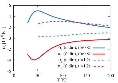
Figure 5: (color online) Temperature dependence of the thermal expansion in the Mott insulating phase. Note the non-monotonic behavior and the large anisotropy. Indeed, in the $b$ direction, thermal contraction rather than expansion occurs. The maximum magnitude occurs at approximately the same temperature as that for which the specific heat and magnetic susceptibility are a maximum (compare Figure S1 of Ref. Kokalj and McKenzie, 2013). The solid curves ($t^{\prime}=0.8t$ and $U=8t$) can be compared to experimental results for $\kappa$-(BEDT-TTF)₂Cu₂(CN)₃ shown in Fig. 1 in Ref. Manna et al., 2010. The results are quite sensitive to the parameter values and proximity to the Mott transition. This is seen by comparing the dashed curves ($t^{\prime}=1.2t$). The parameter values used are described in the text.

In Fig. 5 we show an estimate of the thermal expansion coefficients for the insulating phase and parameters ($t^{\prime}=0.8t$, $U=8t$) that correspond to $\kappa$-(BEDT-TTF)₂Cu₂(CN)₃, and can be compared to experimental data shown in Fig. 1 of Ref. Manna et al., 2010. The calculated magnitude of about $5\times 10^{-6}$/K at 50 K is approximately one fifth of the measured value. We discuss possible explanations of this discrepancy later. As in experiment we observe a strong anisotropy with maximum around 50 K, but the sign of the anisotropy is opposite to the experimental one at such $T$. Interestingly, a similar $T$ dependence with the right absolute values is experimentally observed as a very low $T$ ($\sim 6$ K) anomaly (see Fig. 2 in Ref. Manna et al., 2010), but for agreement our $T$ scale would need to be reduced by a factor of 10, suggesting that this involves different physics beyond our calculations, such as transition into some type of spin liquid phase.

Our results in Fig. 5 have significantly different $T$-dependencies for the thermal expansion coefficients in $c$ ($t$) and $b$ ($t^{\prime}$) directions due to anisotropy in the bond orders shown in Fig. 3, originating in the anisotropy $t^{\prime}=0.8t$ and since variation of the different lattice constant changes differently $t$ and $t^{\prime}$ (Eqs. 11, 12). Low temperature experimental results shown in Fig. 1 of Ref. Manna et al., 2010 show a strong difference in the $T$-dependence between the $b$ and $c$ directions, suggesting that, if they originate from the electronic degrees of freedom, the proper electronic model should have notable $t$-$t^{\prime}$ asymmetry, or that the dependence of $t$ and $t^{\prime}$ on the lattice constants $c$ and $b$ is strongly asymmetric. The anisotropy $\alpha_{c}-\alpha_{b}$ in our results shown in Fig. 5 has the opposite sign to experiment. Taking $t^{\prime}\sim 1.2t>t$ changes the sign of our $\alpha_{c}-\alpha_{b}$ results, making the comparison to experiment better. Change of the sign of the thermal expansion by increasing $t^{\prime}$ above the isotropic point ($t^{\prime}=t$) originates in moving away from maximal frustration (and therefore maximal entropy). This also involves moving away from the isotropic point for which the temperature dependence of both $\langle\hat{T}_{1}\rangle$ and $\langle\hat{T}_{2}\rangle$ is essentially the same (apart from a factor of 2) due to symmetry (compare Figure 3).

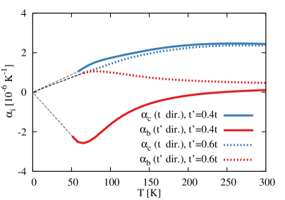
Figure 6: (color online) Temperature dependence of the thermal expansion in the metallic phase ($U=4t$). These results can be compared to Fig. 5a and 5b in Ref. Müller et al., 2002 with the $t^{\prime}=0.4t$ results more relevant for Fig. 5a ($\kappa$-Br) and $t^{\prime}=0.6t$ results more relevant for Fig. 5b ($\kappa$-NCS). The dashed lines are linear extrapolations to zero temperature, as expected for a Fermi liquid. Note that $t^{\prime}=0.4t$ is closer to the Mott insulating phase than $t^{\prime}=0.6t$ (compare Fig. 3 in Ref. Kokalj and McKenzie, 2013). Our $\alpha_{c}$ ($\alpha_{b}$) should be compared to the experimental data shown as full squares (empty circles) in Fig. 5 in Ref. Müller et al., 2002. Our calculated values are about 5-10 times smaller than the measured values. As in experiment we observe for $T\sim 60$ K larger anisotropy ($\alpha_{c}-\alpha_{b}$) for $t^{\prime}=0.4t$ than for $t^{\prime}=0.6t$ with the right sign for $t^{\prime}=0.4t$. We observe a maximum magnitude at $T\sim T_{\textrm{coh}}\sim 60$ K, suggesting that the experimental anomalies at $T\sim 50$ K could have an electronic origin, although the observed increase (decrease) of $\alpha_{c}$ for $\kappa$-Br ($\kappa$-NCS) at such temperature is inconsistent with our results. We use the same parameter values and approximations as for Fig. 5.

In Fig. 6 we show our estimate of the electronic contribution to the thermal expansion for the metallic phase of organic charge transfer salts. Similar to the experimental data, our results show a maximum at $T\sim 60$ K and suggest that the experimentally observed anomalies (see Fig. 5 in Ref. Müller et al., 2002) could have an electronic origin. On the other hand, in Fig. 6 we observe larger anisotropy $(\alpha_{c}-\alpha_{b})$ for $t^{\prime}=0.4t$ than for $t^{\prime}=0.6t$, which is in agreement with experimentally observed larger ($\alpha_{a}-\alpha_{c}$) for $\kappa$-(H₈-ET)₂Cu[N(CN)₂]Br ($\kappa$-Br) shown in Fig. 5a in Ref. Müller et al., 2002 than ($\alpha_{c}-\alpha_{b}$) for $\kappa$-(D₈-ET)₂Cu(NCS)₂ ($\kappa$-NCS) shown in Fig. 5b in Ref. Müller et al., 2002. We note that in $\kappa$-(H₈-ET)₂Cu[N(CN)₂]Br $t^{\prime}\sim 0.4t$ while in $\kappa$-(D₈-ET)₂Cu(NCS)₂ $t^{\prime}\sim 0.6t$ Kandpal et al. (2009).

IV.3 Sign of the hopping integrals

We note that for comparison with the organics in Figs. 5 and 6 we used positive $t$ and $t^{\prime}$ for the Hubbard model defined by Eq. (7), while with respect to our definition DFT based calculations suggest they are both negative Kandpal et al. (2009). This is not a problem, since changing the signs of both $t$ and $t^{\prime}$ corresponds at half-filling to a particle-hole transformation and leads to the same result due to a double sign change, e.g., $\partial\langle\hat{T}_{1}\rangle/\partial T\to-\partial\langle\hat{T}_{1}\rangle/\partial T$ and $\partial t/\partial c\to-\partial t/\partial c$. On the other hand, Refs. Nakamura et al., 2009; Koretsune and Hotta, 2014 suggest negative $t^{\prime}/t$ which could affect the results but actually also $t^{\prime}/t\to-t^{\prime}/t$ corresponds to a particle-hole transformation with an additional $k$-space shift of $(\pi,\pi)$ (considering the equivalent square lattice with one diagonal hopping $t’$). This again does not change the results for thermal expansion. On the other hand, such particle-hole transformations are important for the sign of the thermopower Kokalj and McKenzie (2014).

IV.4 Future challenges

We now discuss several possible improvements to our theoretical description that we leave as future challenges. First it is clear from discussion of Eq. (6) and furthermore from discussion of anisotropic effects in Appendix A and Eq. (21) therein that for an anisotropic materials like the organics the stiffness tensor $C_{ijkl}$ can be strongly anisotropic with several important elastic constants that are not known at a moment, but may be experimentally accessible. For example, adding Poisson’s ratios to known Young’s moduli and extracting also other elastic constants would allow for a full tensor description. This is not just of interest for the study of thermal expansion, but also on its own, since also stiffness tensor has notable electronic contributions. These have been already observed as lattice softening, e.g., via sound velocity Fournier et al. (2003); Hassan et al. (2005), which becomes substantial (up to 50%) close to the metal-insulator transition (MIT) and in addition suggests critical behaviour at the end of the first-order line, leading to a diverging $\partial^{2}\Omega/\partial t^{2}$ related to $\partial^{2}\Omega/\partial l_{i}^{2}$ [see Eq. (20)]. One should however keep in mind, that the MIT is experimentally observed to be weakly first order in the organics Limelette et al. (2003) but its order in a Hubbard model at half filling is still controversial Yamada (2014); Yoshioka et al. (2009); Mishmash et al. (2014); Yang et al. (2010). In our analysis we do not include these lattice softening effects (reduced Young’s modulus) close to the metal-insulator transition, but their inclusion would increase our $\alpha_{i}$ by roughly a factor of two, making the electronic contribution to $\alpha_{i}$ larger and more important and would improve the comparison to experiment (see in particular the discussion of Fig. 6).

Another challenge is to obtain the dependence of the Hubbard model parameters ($t$, $t^{\prime}$ and $U$) on all lattice constants $a_{i}$ and on all structural parameters, including the angles and orientation of molecules. These dependencies are not easy to obtain, and simple Eqs. (11-13) could be greatly improved with more elaborate DFT calculations or studies such as in Refs. Mori, 1998; Mori et al., 1999. In particular Fig. 2 in Ref. Mori et al., 1999 shows that in various salts the different angle between ET molecules is directly connected to the lattice constants, which suggests that this angle is an important structural parameter and that it possibly varies also with temperature and applied stress. Therefore DFT calculations, which would in addition to intermolecular spacing relax also angles between molecules, could be valuable and present a future challenge. DFT could connect changes of $H_{el}$ parameters to changes of structural parameters with the complete tensor. This would further facilitate the full tensor description of electronic contribution to thermal expansion and elastic constants.

V Conclusions

We have shown how the electronic contribution to the thermal expansion is related to the electronic degrees of freedom via the parameters ($t$, $t^{\prime}$ and $U$) in a Hubbard model and temperature derivatives of known quantities (bond orders and double occupancy). The values of thermal expansion coefficients are further governed by the relation of model parameters to lattice (structural) constants and by elasticity constants.

The electronic contribution to the thermal expansion is large with strong orientational and non-monotonic temperature dependence. Furthermore, we showed that correlations strongly increase the electronic contribution and by estimating it for organic charge transfer salts we showed that it can provide a qualitative understanding of experimental data for temperatures below 100 K. In particular, contrary to suggestions in Ref. Müller et al., 2002, the anomalies around 50 K may not be lattice anomalies or structural phase transitions, rather they could originate from the electronic contribution, and be due to the bad metal - Fermi liquid crossover.

It should be stressed that also phononic contribution to the thermal expansion may play an important role at quite low $T$, which is suggested by large phononic contribution to specific heat (see Ref. Yamashita et al., 2008, 2011 and the Supplement of Ref. Kokalj and McKenzie, 2013) and in turn to entropy relevant for thermal expansion [Eq. (3)]. Therefore the study of lattice vibrations (e.g., anharmonic effects, orientational dependence or the Grüneisen parameter Ashcroft and Mermin (1976)) and the estimates of their contribution to thermal expansion or stiffness tensor may aid our understanding.

Appendix A Anisotropic thermal expansion

We discuss thermal expansion here in terms of a grand potential $\Omega$, due to its simple connection to the electronic Hamiltonian

$$\exp{(-\beta\Omega)}=\textrm{Tr}[\exp{(-\beta\hat{H}_{el})}],$$ (16)

and its straight forward calculation within FTLM Jaklič and Prelovšek (2000). Thermal expansion coefficients are given by

$$\alpha_{i}\equiv\frac{1}{l_{i}}\left(\frac{\partial l_{i}}{\partial T}\right)_{P,N_{e}},$$ (17)

where $l_{i}$ is a length of a sample in the $i$ ($=x,y$ or $z$) direction and can be exchanged also by a lattice constant $a_{i}$, and where we denoted that experiments are done at constant pressure ($P$) and fixed electron number ($N_{e}$). Since we are interested also in an orientational ($i$) dependence, we first need to generalize the standard mechanical work $-PdV$ to $V^{0}\sum_{i,j}\sigma_{ij}d\varepsilon_{ij}$ with $V^{0}$ being a reference volume, while $\sigma_{ij}$ and $\varepsilon_{ij}$ are stress and strain tensors, respectively. We however simplify our analysis by considering just normal stress and no shear deformations taking only diagonal terms. $\sigma_{ii}=\sigma_{i}$ is uniaxial stress which equal $-P$ for isotropic pressure and $\varepsilon_{ii}=dl_{i}/l_{i}^{0}$ with $l_{i}^{0}$ denoting reference length. With this we can write mechanical work as $\sum_{i}\sigma_{i}V^{0}dl_{i}/l_{i}^{0}$. This brings us to $\Omega=\Omega(T,l_{i},\mu)$ and $d\Omega=-SdT+\sum_{i}\sigma_{i}V^{0}dl_{i}/l_{i}^{0}-N_{e}d\mu$, where for a fixed $N_{e}$ one needs to adjust the chemical potential, $\mu=\mu(T,l_{i},N_{e})$. From $\Omega$ one can obtain the equation of state which for usual work ($-PdV$) reads $-P=(\partial\Omega/\partial V)_{T,\mu}$ but with our generalized work the three equations of state (for $i=x,y,z$) are

$$\sigma_{i}=\frac{l_{i}^{0}}{V^{0}}\left(\frac{\partial\Omega}{\partial l_{i}}\right)_{T,l_{j\neq i},\mu}.$$ (18)

Taking the full derivative of equation of state for fixed $N_{e}$ in the case of usual work ($-PdV$) one obtains differential equation of state $-dP=(\frac{\partial}{\partial T}(\frac{\partial\Omega}{\partial V})_{T,\mu})_{V,N_{e}}dT+(\frac{\partial}{\partial V}(\frac{\partial\Omega}{\partial V})_{T,\mu})_{T,N_{e}}dV$, which when compared to $dV/V=\beta dT-\kappa_{T}dP$ gives expression for isothermal bulk compressibility $\kappa_{T}^{-1}=V(\frac{\partial}{\partial V}(\frac{\partial\Omega}{\partial V})_{T,\mu})_{T,N_{e}}$ and volume thermal expansion $\beta=\kappa_{T}(\frac{\partial}{\partial T}(\frac{\partial\Omega}{\partial V})_{T,\mu})_{V,N_{e}}$ in terms of $\Omega$. Similarly taking full differentials of Eq. (18) leads to differential equations of states

$$d\sigma_{i} \!\!= \!\!\frac{l_{i}^{0}}{V^{0}}\Big{(}\frac{\partial}{\partial T}\!\Big{(}\frac{\partial\Omega}{\partial l_{i}}\Big{)}_{\!T,l_{k\neq i},\mu}\Big{)}_{\!l_{j},N_{e}}\!dT\!+\!\sum_{j}C_{ij}\frac{dl_{j}}{l_{j}^{0}},$$ (19)

$$C_{ij} \!\!= \!\!\frac{l_{i}^{0}l_{j}^{0}}{V^{0}}\Big{(}\frac{\partial}{\partial l_{j}}\!\Big{(}\frac{\partial\Omega}{\partial l_{i}}\Big{)}_{\!T,l_{k\neq i},\mu}\Big{)}_{\!T,l_{k\neq j},N_{e}}.$$ (20)

From above Eq. (19) it is clear that a small change of strain $dl_{j}/l_{j}^{0}=\varepsilon_{j}$ leads to a small change of stress $d\sigma_{i}=\tilde{\sigma}_{i}$, which are at constant temperature ($dT=0$) related by $\tilde{\sigma}_{i}=C_{ij}\varepsilon_{j}$ or with expanded indices $\tilde{\sigma}_{ii}=C_{iijj}\varepsilon_{jj}$, namely by Hook’s law. Now we recognise $C_{ij}$ or $C_{iijj}$ as a stiffness tensor, which depends on material’s elastic constants, and has replaced $\kappa_{T}^{-1}$. The symmetry of $C_{ij}$ is discussed in Appendix C.

Thermal expansion coefficients can now be expressed as

$$\alpha_{i}=\sum_{j}(C^{-1})_{i,j}\frac{-l_{j}^{0}}{V^{0}}\Big{(}\frac{\partial}{\partial T}\Big{(}\frac{\partial\Omega}{\partial l_{j}}\Big{)}_{T,l_{k\neq j},\mu}\Big{)}_{l_{k},N_{e}},$$ (21)

and we further for clarity simplify our calculation by assuming that Poisson’s ratio is small which makes $C^{-1}$ diagonal, $(C^{-1})_{i,j}=(1/E_{i})\delta_{ij}$ with $E_{i}$ being Young’s modulus in $i$ direction.

Similarly one can show that $l_{i}$- and $T$-derivatives of $\Omega$ in Eq. (21), can be replaced with $l_{i}$ derivative of entropy $S$. See Appendix B for more detail.

$$\alpha_{i}=\frac{1}{E_{i}}\frac{l_{i}^{0}}{V^{0}}\Big{(}\frac{\partial S}{\partial l_{i}}\Big{)}_{T,l_{k\neq i},N_{e}}.$$ (22)

Further more, since $E_{i}>0$ the sign of $\alpha_{i}$ is determined by the entropy derivative and therefore whether the change of $l_{i}$ (or in turn some electronic model parameter, see Eqs. (12) and (11)) increases or decreases the entropy. For maximally frustrated systems the low-$T$ entropy is expected to be maximal and therefore the sign of $\alpha_{i}$ can help determining whether one is with a certain parameter above or below the maximal frustration.

Appendix B Relation of thermal expansion to entropy via grand potential

Here we show that the $T$ and $l_{i}$ derivative of $\Omega$, one at fixed $N_{e}$ and the other at fixed $\mu$, appearing in Eq. (21) for thermal expansion can be expressed as $l_{i}$ derivative of entropy. Such relation can be shown with the use of Helmholtz free energy $F$, but here we show it by using $\Omega$.

$$\Big{(}\frac{\partial}{\partial T}\Big{(}\frac{\partial\Omega}{\partial l_{i}}\Big{)}_{T,l_{k\neq i},\mu}\Big{)}_{l_{k},N_{e}} \!\!= \!\!\Big{(}\frac{\partial^{2}\Omega}{\partial T\partial l_{i}}\Big{)}_{l_{k\neq i},\mu}$$ (23)

$$\!\!+ \!\!\Big{(}\frac{\partial^{2}\Omega}{\partial\mu\partial l_{i}}\Big{)}_{T,l_{k\neq i}}\Big{(}\frac{\partial\mu}{\partial T}\Big{)}_{l_{k},N_{e}}$$

$$-\Big{(}\frac{\partial S}{\partial l_{i}}\Big{)}_{T,l_{k\neq i},N_{e}} \!\!= \!\!\Big{(}\frac{\partial^{2}\Omega}{\partial l_{i}\partial T}\Big{)}_{l_{k\neq i},\mu}$$ (24)

$$\!\!+ \!\!\Big{(}\frac{\partial^{2}\Omega}{\partial\mu\partial T}\Big{)}_{l_{k}}\Big{(}\frac{\partial\mu}{\partial l_{i}}\Big{)}_{T,l_{k\neq i},N_{e}}.$$

Since $-N_{e}=(\partial\Omega/\partial\mu)_{T,l_{i}}$ we can write

$$\Big{(}\frac{\partial}{\partial l_{i}}\Big{(}\frac{\partial\Omega}{\partial\mu}\Big{)}_{T,l_{k}}\Big{)}_{T,l_{k\neq i},N_{e}} \!= \!0\!=\!\!\Big{(}\frac{\partial^{2}\Omega}{\partial\mu\partial l_{i}}\Big{)}_{T,l_{k\neq i}}$$ (25)

$$\!\!+ \!\!\Big{(}\frac{\partial^{2}\Omega}{\partial^{2}\mu}\Big{)}_{\!T,l_{k}}\!\!\Big{(}\frac{\partial\mu}{\partial l_{i}}\Big{)}_{\!T,l_{k\neq i},N_{e}}$$

$$\Big{(}\frac{\partial}{\partial T}\Big{(}\frac{\partial\Omega}{\partial\mu}\Big{)}_{T,l_{k}}\Big{)}_{l_{k},N_{e}} \!= \!0\!=\!\!\Big{(}\frac{\partial^{2}\Omega}{\partial\mu\partial T}\Big{)}_{l_{k}}$$ (26)

$$\!\!+ \!\!\Big{(}\frac{\partial^{2}\Omega}{\partial^{2}\mu}\Big{)}_{\!T,l_{k}}\!\!\Big{(}\frac{\partial\mu}{\partial T}\Big{)}_{\!l_{k},N_{e}}$$

Using Eqs. (25) and (26) in Eqs. (23) and (24) makes it clear that both expressions [Eqs. (23) and (24)] are equal and therefore $\alpha_{i}$ in Eq. (21) can be connected to the derivative of entropy.

Appendix C Symmetry of $C_{ij}$

By symmetry $C_{ij}$ should equal $C_{ji}$, which is not directly seen from Eq. (20) since for example $i$-derivative of $\Omega$ is taken at fixed $\mu$, while $j$-derivative is taken at fixed $N_{e}$. We show here for example, that $C_{xy}$ given with Eq. (20) obeys the symmetry. Keeping in mind that $\Omega=\Omega(T,l_{i},\mu)$ and for fixed $N_{e}$, $\mu=\mu(T,l_{i},N_{e})$ we can write out the first term

$$\Big{(}\frac{\partial}{\partial l_{y}}\Big{(}\frac{\partial\Omega}{\partial l_{x}} \Big{)}_{T,l_{k\neq x},\mu}\Big{)}_{T,l_{k\neq y},N_{e}}=\Big{(}\frac{\partial^{2}\Omega}{\partial l_{y}\partial l_{x}}\Big{)}_{T,l_{k\neq x,y},\mu}$$ (27)

$$+\Big{(}\frac{\partial^{2}\Omega}{\partial l_{x}\partial\mu}\Big{)}_{T,l_{k\neq x}}\Big{(}\frac{\partial\mu}{\partial l_{y}}\Big{)}_{T,l_{k\neq y},N_{e}}.$$

By using $-N_{e}=(\partial\Omega/\partial\mu)_{T,l_{i}}$ one obtaines

$$\Big{(}\frac{\partial}{\partial l_{x}}\Big{(}\frac{\partial\Omega}{\partial\mu}\Big{)}_{T,l_{i}}\Big{)}_{T,l_{k\neq x},N_{e}}=0=\Big{(}\frac{\partial^{2}\Omega}{\partial l_{x}\partial\mu}\Big{)}_{T,l_{k\neq x}}$$

$$+\Big{(}\frac{\partial^{2}\Omega}{\partial\mu^{2}}\Big{)}_{T,l_{i}}\Big{(}\frac{\partial\mu}{\partial l_{x}}\Big{)}_{T,l_{k\neq x},N_{e}}.$$ (28)

Using this relation in Eq. (27) and then further in Eq. (20) one gets

$$C_{xy} = \frac{l_{x}l_{y}}{V}\Big{[}\Big{(}\frac{\partial^{2}\Omega}{\partial l_{x}\partial l_{y}}\Big{)}_{T,l_{k\neq x,y},\mu}$$

$$- \Big{(}\frac{\partial^{2}\Omega}{\partial\mu^{2}}\Big{)}_{T,l_{i}}\Big{(}\frac{\partial\mu}{\partial l_{x}}\Big{)}_{T,l_{k\neq x},N_{e}}\Big{(}\frac{\partial\mu}{\partial l_{y}}\Big{)}_{T,l_{k\neq y},N_{e}}\Big{]}.$$

From this it is obvious that $C_{xy}=C_{yx}$ and the symmetry is obeyed.

References

- White (1993) G. White, Contemp. Phys. 34, 193 (1993).
- Lacerda et al. (1989) A. Lacerda, A. de Visser, P. Haen, P. Lejay, and J. Flouquet, Phys. Rev. B 40, 8759 (1989).
- Müller et al. (2002) J. Müller, M. Lang, F. Steglich, J. A. Schlueter, A. M. Kini, and T. Sasaki, Phys. Rev. B 65, 144521 (2002).
- de Souza et al. (2007) M. de Souza, A. Brühl, C. Strack, B. Wolf, D. Schweitzer, and M. Lang, Phys. Rev. Lett. 99, 037003 (2007).
- Manna et al. (2010) R. S. Manna, M. de Souza, A. Brühl, J. A. Schlueter, and M. Lang, Phys. Rev. Lett. 104, 016403 (2010).
- de Souza and Pouget (2013) M. de Souza and J.-P. Pouget, J. Phys.: Condens. Matter 25, 343201 (2013).
- Meingast et al. (2012) C. Meingast, F. Hardy, R. Heid, P. Adelmann, A. Böhmer, P. Burger, D. Ernst, R. Fromknecht, P. Schweiss, and T. Wolf, Phys. Rev. Lett. 108, 177004 (2012).
- Hardy et al. (2013) F. Hardy, A. E. Böhmer, D. Aoki, P. Burger, T. Wolf, P. Schweiss, R. Heid, P. Adelmann, Y. X. Yao, G. Kotliar, J. Schmalian, and C. Meingast, Phys. Rev. Lett. 111, 027002 (2013).
- Johnston et al. (1999) D. Johnston, C. Swenson, and S. Kondo, Phys. Rev. B 59, 2627 (1999).
- Zhu et al. (2003) L. Zhu, M. Garst, A. Rosch, and Q. Si, Phys. Rev. Lett. 91, 066404 (2003).
- Müller et al. (2000) J. Müller, M. Lang, F. Steglich, J. A. Schlueter, A. M. Kini, U. Geiser, J. Mohtasham, R. W. Winter, G. L. Gard, T. Sasaki, and N. Toyota, Phys. Rev. B 61, 11739 (2000).
- Fournier et al. (2003) D. Fournier, M. Poirier, M. Castonguay, and K. D. Truong, Phys. Rev. Lett. 90, 127002 (2003).
- Hassan et al. (2005) S. R. Hassan, A. Georges, and H. R. Krishnamurthy, Phys. Rev. Lett. 94, 036402 (2005).
- Zacharias et al. (2012) M. Zacharias, L. Bartosch, and M. Garst, Phys. Rev. Lett. 109, 176401 (2012).
- Powell and McKenzie (2011) B. J. Powell and R. H. McKenzie, Rep. Prog. Phys. 74, 056501 (2011).
- Shimizu et al. (2003) Y. Shimizu, K. Miyagawa, K. Kanoda, M. Maesato, and G. Saito, Phys. Rev. Lett. 91, 107001 (2003).
- Merino et al. (2008) J. Merino, M. Dumm, N. Drichko, M. Dressel, and R. H. McKenzie, Phys. Rev. Lett. 100, 086404 (2008).
- Yu et al. (1991) R. C. Yu, J. M. Williams, H. H. Wang, J. E. Thompson, A. M. Kini, K. D. Carlson, J. Ren, M.-H. Whangbo, and P. M. Chaikin, Phys. Rev. B 44, 6932 (1991).
- Deng et al. (2013) X. Deng, J. Mravlje, R. Žitko, M. Ferrero, G. Kotliar, and A. Georges, Phys. Rev. Lett. 110, 086401 (2013).
- Lang et al. (2008) M. Lang, M. de Souza, A. Brühl, C. Strack, B. Wolf, and D. Schweitzer, Physica B 403, 1384 (2008).
- Jaklič and Prelovšek (2000) J. Jaklič and P. Prelovšek, Adv. Phys. 49, 1 (2000).
- Kokalj and McKenzie (2013) J. Kokalj and R. H. McKenzie, Phys. Rev. Lett. 110, 206402 (2013).
- Shimizu et al. (2011) Y. Shimizu, M. Maesato, and G. Saito, J. Phys. Soc. Jpn. 80, 074702 (2011).
- Mori (1998) T. Mori, Bull. Chem. Soc. Jpn. 71, 2509 (1998).
- Mori et al. (1999) T. Mori, H. Mori, and S. Tanaka, Bull. Chem. Soc. Jpn. 72, 179 (1999).
- Kondo et al. (2003) R. Kondo, S. Kagoshima, and M. Maesato, Phys. Rev. B 67, 134519 (2003).
- Kandpal et al. (2009) H. C. Kandpal, I. Opahle, Y.-Z. Zhang, H. O. Jeschke, and R. Valentí, Phys. Rev. Lett. 103, 067004 (2009).
- Jeschke et al. (2012) H. O. Jeschke, M. de Souza, R. Valentí, R. S. Manna, M. Lang, and J. A. Schlueter, Phys. Rev. B 85, 035125 (2012).
- Li et al. (2014) G. Li, A. E. Antipov, A. N. Rubtsov, S. Kirchner, and W. Hanke, Phys. Rev. B 89 (2014).
- Laubach et al. (2014) M. Laubach, R. Thomale, W. Hanke, and G. Li, arXiv:1401.8198 [cond-mat] (2014).
- Merino and McKenzie (2000) J. Merino and R. H. McKenzie, Phys. Rev. B 61, 7996 (2000).
- Nakamura et al. (2009) K. Nakamura, Y. Yoshimoto, T. Kosugi, R. Arita, and M. Imada, J. Phys. Soc. Jpn. 78, 083710 (2009).
- Rahal et al. (1997) M. Rahal, D. Chasseau, J. Gaultier, L. Ducasse, M. Kurmoo, and P. Day, Acta Crystallogr. Sect. B: Struct. Sci. 53, 159 (1997).
- Koretsune and Hotta (2014) T. Koretsune and C. Hotta, Phys. Rev. B 89, 045102 (2014).
- Kokalj and McKenzie (2014) J. Kokalj and R. H. McKenzie, arXiv:1410.0830 [cond-mat] (2014).
- Limelette et al. (2003) P. Limelette, P. Wzietek, S. Florens, A. Georges, T. A. Costi, C. Pasquier, D. Jérome, C. Mézière, and P. Batail, Phys. Rev. Lett. 91, 016401 (2003).
- Yamada (2014) A. Yamada, Phys. Rev. B 89, 195108 (2014).
- Yoshioka et al. (2009) T. Yoshioka, A. Koga, and N. Kawakami, Phys. Rev. Lett. 103, 036401 (2009).
- Mishmash et al. (2014) R. V. Mishmash, I. Gonzalez, R. G. Melko, O. I. Motrunich, and M. P. A. Fisher, arXiv:1403.4258 [cond-mat] (2014).
- Yang et al. (2010) H.-Y. Yang, A. M. Läuchli, F. Mila, and K. P. Schmidt, Phys. Rev. Lett. 105, 267204 (2010).
- Yamashita et al. (2008) S. Yamashita, Y. Nakazawa, M. Oguni, Y. Oshima, H. Nojiri, Y. Shimizu, K. Miyagawa, and K. Kanoda, Nat. Phys. 4, 459 (2008).
- Yamashita et al. (2011) S. Yamashita, T. Yamamoto, Y. Nakazawa, M. Tamura, and R. Kato, Nat. Commun. 2, 275 (2011).
- Ashcroft and Mermin (1976) N. W. Ashcroft and N. D. Mermin, Solid State Physics, 1st ed. (Thomson Learning, Toronto, 1976).