SNUTP14-012

Defect branes as Alice strings

Takashi Okada and Yuho Sakatani

^∗Theoretical Biology Laboratory, RIKEN,
Wako 351-0198, JAPAN

^†Department of Physics and Astronomy,
Seoul National University, Seoul 151-747, KOREA

There exist various defect-brane backgrounds in supergravity theories which arise as the low energy limit of string theories. These backgrounds typically have non-trivial monodromies, and if we move a charged probe around the center of a defect, its charge will be changed by the action of the monodromy. During the process, the charge conservation law seems to be violated. In this paper, to resolve this puzzle, we examine a dynamics of the charge changing process and show that the missing charge of the probe is transferred to the background. We then explicitly construct the resultant background after the charge transfer process by utilizing dualities. This background has the same monodromy as the original defect brane, but has an additional charge which does not have any localized source. In the literature, such a charge without localized source is known to appear in the presence of Alice strings. We argue that defect branes can in fact be regarded as a realization of Alice strings in string theory and examine the charge transfer process from that perspective.

1 Introduction

String theory has various defect branes (or codimension-two branes), including the well-known D7-brane and various exotic branes. In the supergravity description, some of the corresponding backgrounds are called non-geometric backgrounds or U-folds [1], since the transition functions between coordinate patches are given by U-duality transformations. In particular, the authors in [2] pointed out that the background of $5_{2}^{2}$-branes [3] has a T-duality monodromy and it is a concrete example of non-geometric backgrounds in string theory.

The non-trivial monodromies of defect branes, which is familiar for a D7-brane, generally raise a perplexing problem related to the charge conservation law. Let us consider a charged probe brane in a defect-brane background. If we move the probe around the center of the defect, its charge will change due to the action of the monodromy. Where does the original charge of the probe go and how is the charge conservation law kept intact? In [4], it was proposed that the charge is indeed conserved if we measure the charge by using the Page charge [5, 6, 4], which is one of the possible definitions of charge. However, in defect-brane backgrounds, the definition of the (Page) charge depends on the choice of a cycle for a flux integral (see [4] and section 3.2). Thus, it is desirable to define the charge in a consistent manner to analyze the (apparent) charge changing phenomena.

In the literature, the similar issue was discussed in a certain class of $(1+3)$-dimensional gauge theories which admit vortex solutions with non-trivial monodromies [7, 8, 9]. One of the most famous and studied example is a vortex called an Alice string [7], whose monodromy is given by a charge conjugation. That is, after a particle with charge $q$ goes around an Alice string, the sign of its charge flips. In the presence of Alice strings, “a charge with no localized source,” called a Cheshire charge [8, 9], plays an important role in the discussion of the charge conservation law. In this paper, we will examine an analogy between Alice strings and defect branes in string theory (see [16] for an earlier study on a realization of Alice string in string theory).

In order to discuss the issue of the charge conservation law in defect-brane backgrounds more concretely, let us consider a Kaluza-Klein (KK) vortex (or smeared KK monopole) background [17, 18, 3] as an example. A key feature of the KK-vortex background different from other defect-brane backgrounds is that the monodromy of the KK-vortex background is just a coordinate transformation, which enables us to understand the charge changing phenomena geometrically. The KK-vortex background is given by

$${\mathrm{d}}s^{2} =-{\mathrm{d}}t^{2}+H(r)\,\bigl{(}{\mathrm{d}}r^{2}+r^{2}\,{\mathrm{d}}\theta^{2}+{\mathrm{d}}x_{3}^{2}\bigr{)}+H^{-1}(r)\,\bigl{[}{\mathrm{d}}x^{4}-\sigma\,(\theta/2\pi)\,{\mathrm{d}}x^{3}\bigr{]}^{2}+{\mathrm{d}}x^{2}_{56789}\,,$$ (1.1)

$$\operatorname{e}^{\,2\hat{\phi}} =1\,,\qquad\hat{B}^{(2)}=0\,,\quad H(r)\equiv(\sigma/2\pi)\,\log(r_{\rm c}/r)\,.$$ (1.2)

Here, we defined $\sigma\equiv R_{4}/R_{3}$ where $R_{i}$ ($i=3,\dotsc,9$) is the compactification radius in the $x^{i}$-direction, and $r_{\rm c}$ is a cutoff radius of the geometry; the geometry gives a good description only for $r\ll r_{\rm c}$. If we gather the $x^{3}$-$x^{4}$ components of the metric and $B$-field into the generalized metric of a $4\times 4$ matrix

$$\mathcal{H}^{-1}\equiv\begin{pmatrix}\hat{G}^{-1}&-\hat{G}^{-1}\,\hat{B}\cr\hat{B}\,\hat{G}^{-1}&\hat{G}-\hat{B}\,\hat{G}^{-1}\,\hat{B}\end{pmatrix}\,,$$ (1.3)

the monodromy around the center, $r=0$, is given by the matrix $\Omega_{{\rm KKM}}$:

$$\mathcal{H}^{-1}(\theta=2\pi)=\Omega_{{\rm KKM}}^{\rm T}\,\mathcal{H}^{-1}(\theta=0)\,\Omega_{{\rm KKM}}\,,$$ (1.4)

$$\Omega_{{\rm KKM}}\equiv\begin{pmatrix}{\boldsymbol{\omega}}^{\rm T}&\mathbf{0}\cr\mathbf{0}&{\boldsymbol{\omega}}^{-1}\cr\end{pmatrix}\,,\quad{\boldsymbol{\omega}}\equiv\begin{pmatrix}1&0\cr\sigma&\,1\,\cr\end{pmatrix}\,.$$ (1.5)

The monodromy matrix $\Omega_{{\rm KKM}}$ characterizes the existence of the KK vortex at the center.

Due to the existence of the non-trivial monodromy, if we put a probe string with ${\rm F}1(3)$ charge and move it once around the center counterclockwise, its charge will change as

$$\footnotesize\begin{pmatrix}(1/R_{3})\times\#{\rm P}(3)\cr(1/R_{4})\times\#{\rm P}(4)\cr(R_{3}/l_{s}^{2})\times\#{\rm F}1(3)\cr(R_{4}/l_{s}^{2})\times\#{\rm F}1(4)\end{pmatrix}=\footnotesize\begin{pmatrix}0\cr 0\cr(R_{3}/l_{s}^{2})\times 1\cr 0\end{pmatrix}\ \to\ \Omega_{{\rm KKM}}^{-1}\,\footnotesize\begin{pmatrix}0\cr 0\cr(R_{3}/l_{s}^{2})\times 1\cr 0\end{pmatrix}=\footnotesize\begin{pmatrix}0\cr 0\cr(R_{3}/l_{s}^{2})\times 1\cr(R_{4}/l_{s}^{2})\times 1\end{pmatrix}\,.$$ (1.6)

The change in the winding charge can be understood geometrically; the monodromy $\Omega_{{\rm KKM}}$ of the KK vortex corresponds to the diffeomorphism on a 3-4 torus:

$$x^{\prime 3}=x^{3}\,,\qquad x^{\prime 4}=x^{4}+\sigma\,x^{3}\,.$$ (1.7)

As described in Figure 1 (left), the probe is initially extending along the $x^{3}$-direction.

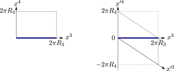
Figure 1: Coordinate system in the 3-4 torus at $\theta=0$ (left) and $\theta=2\pi$ (right). The thick line represents the portrait of the string.

After it goes around the center of the defect, in the above primed coordinates, the probe string extends from $(x^{\prime 3},x^{\prime 4})=(0,\,0)$ to $(2\pi R_{3},\,2\pi R_{4})$ . That is, if we count the winding number using the primed coordinates, the resulting charge is ${\rm F}1(3)+{\rm F}1(4)$, which agrees with (1.6). The reason why we use the primed coordinates for the purpose of measuring the winding charge will be discussed in section 3.2.

If the total charge is to be conserved, we expect that the background after the probe rotated should carry a flux that compensates the charge change of the probe. In this paper, we examine in detail the dynamical process in which the winding charge of a probe string is transferred to the background, and discuss on the charge conservation during this process. Then, we explicitly construct a deformed defect-brane background with an additional charge by utilizing the four-dimensional electric-magnetic duality. We show that the additional charge is exactly the same as that left behind by the probe brane and thus the background can be regarded as the resultant background after the probe goes around the defect.

We also examine the charge transfer process in the $5^{2}_{2}$-brane background. Compared with the KK-vortex, the case is rather difficult to understand geometrically since the monodromy is not the usual coordinate transformation but a T-duality transformation. We will circumvent this obstacle by introducing the double field theory [20, 21, 22, 23, 24, 25].

This paper is organized as follows. In section 2, we consider a probe string rotating around a KK vortex and examine the detailed dynamics of the charge transfer process explained above, based on the analysis of [26]. In section 3, we review the notions of Alice strings and Cheshire charges and discuss their relevance to defect branes in string theory. In section 4, we review the construction of the KK-dyon solution following [27], which uses the electric-magnetic duality in four-dimensional theory. We then find that this background has F1 charges which do not have localized source, just like Cheshire charges. Moreover, using a smearing procedure, we construct a dyonic KK-vortex solution and discuss its relevance to the charge transfer process considered in section 2. In section 5, we first construct the $5^{2}_{2}$ background with F1 charges (with no localized source) by using a duality transformation and show that it is a $T$-fold, whose monodromy is the same as that of the pure $5_{2}^{2}$ background. Then, we consider the charge transfer process in the $5^{2}_{2}$ background, and argue that the change of charge can be geometrically understood if we describe the $5^{2}_{2}$ background as a doubled geometry. In section 6, using successive $U$-dualities, we obtain various defect-brane backgrounds with Cheshire charges. We then find another construction of such backgrounds without the use of the electric-magnetic duality in four dimensions. Section 7 is devoted to discussions and conclusion.

2 Monodromy and charge transfer process

As we discussed in the introduction, once a probe brane moves around a defect brane, it is natural to expect that some charges are transferred from the probe brane to the background. In this section, we examine the charge transfer process following the analysis of [26].

Concretely, we consider a probe string with a winding charge, ${\rm F}1(4)$, rotating around the center of the KK-vortex background (1.2). In the following, we dimensionally reduce the $x^{4},\dotsc,x^{9}$-directions, and thus the probe string here is smeared along these directions (i.e. it has codimension two). For generality, we make the following ansatz for the background fields:

$${\mathrm{d}}s^{2} =\hat{G}_{MN}\,{\mathrm{d}}x^{M}\,{\mathrm{d}}x^{N}=g_{\mu\nu}\,{\mathrm{d}}x^{\mu}\,{\mathrm{d}}x^{\nu}+G_{44}\,\bigl{(}{\mathrm{d}}x^{4}+A^{4}\bigr{)}^{2}+{\mathrm{d}}x^{2}_{5\cdots 9}\,,$$ (2.1)

$$\hat{B}^{(2)} =\frac{1}{2}\,\hat{B}^{(2)}_{MN}\,{\mathrm{d}}x^{M}\wedge{\mathrm{d}}x^{N}=\frac{1}{2}\,\bigl{(}B_{\mu\nu}+A^{4}_{\mu}\,A_{4\nu}\bigr{)}\,{\mathrm{d}}x^{\mu}\wedge{\mathrm{d}}x^{\nu}+A_{4}\wedge\bigl{(}{\mathrm{d}}x^{4}+A^{4}\bigr{)}$$

$$\bigl{[}A^{4} =A^{4}_{\mu}\,{\mathrm{d}}x^{\mu}\,,\quad A_{4}=A_{4\mu}\,{\mathrm{d}}x^{\mu}\,,\quad\mathcal{A}^{I}\equiv\bigl{(}A^{4}\,,\ A_{4}\bigr{)}^{\rm T}\,,\quad\mu,\,\nu=0,\dotsc,3\,\bigr{]}\,.$$ (2.2)

By considering a compactification to four dimensions, we obtain the following action:

$$S =S_{\rm bulk}+S_{\rm probe}\,,$$ (2.3)

$$S_{\rm bulk} \equiv\frac{1}{2\kappa_{4}^{2}}\,\int{\mathrm{d}}^{4}x\,\sqrt{-g}\operatorname{e}^{\,-2\phi}\Bigl{[}R-\frac{1}{12}\,H_{\mu\nu\rho}\,H^{\mu\nu\rho}-\frac{1}{4}(M^{-1})_{IJ}\,\mathcal{F}^{I}_{\mu\nu}\,\mathcal{F}^{J\mu\nu}+\cdots\Bigr{]}\,,$$ (2.4)

$$S_{\rm probe} \equiv-\frac{1}{4\pi l_{s}^{2}}\,\int{\mathrm{d}}^{2}\sigma\,{\mathrm{d}}^{4}x\,\delta^{4}(x-X(\boldsymbol{\sigma}))\,\bigl{(}\eta^{ab}\,\hat{G}_{MN}+\epsilon^{ab}\,\hat{B}^{(2)}_{MN}\bigr{)}\,\partial_{a}X^{M}\,\partial_{b}X^{N}$$

$$=-\frac{1}{4\pi l_{s}^{2}}\,\int{\mathrm{d}}^{2}\sigma\,{\mathrm{d}}^{4}x\,\delta^{4}(x-X(\boldsymbol{\sigma}))$$

$$\qquad\qquad\times\Bigl{[}\eta^{ab}\,\bigl{(}h_{ab}+G_{44}\,V_{a}\,V_{b}\bigr{)}+\epsilon^{ab}\,\bigl{(}b_{ab}+A^{4}_{a}\,A_{4b}+2A_{4a}\,V_{b}\bigr{)}\Bigr{]}\,,$$ (2.5)

where $(\boldsymbol{\sigma})=(\sigma^{0},\,\sigma^{1})$ ($0\leq\sigma^{1}\leq 1$) are worldsheet coordinates and we defined

$$\mathcal{F}^{I} \equiv{\mathrm{d}}\mathcal{A}^{I}\,,\quad M^{-1}\equiv\begin{pmatrix}G_{44}&0\cr 0&G_{44}^{-1}\end{pmatrix}\,,\quad H\equiv{\mathrm{d}}B-\frac{1}{2}\,\bigl{(}\mathcal{A}^{4}\wedge\mathcal{F}_{4}+\mathcal{A}_{4}\wedge\mathcal{F}^{4}\bigr{)}\,,$$ (2.6)

$$h_{ab} \equiv g_{\mu\nu}\,\partial_{a}X^{\mu}\,\partial_{b}X^{\nu}\,,\quad V_{a}\equiv\partial_{a}X^{4}+A^{4}_{\mu}\,\partial_{a}X^{\mu}\,,\quad b_{ab}\equiv B_{\mu\nu}\,\partial_{a}X^{\mu}\,\partial_{b}X^{\nu}\,,$$ (2.7)

and $\epsilon^{10}=-\epsilon^{01}=1$, and assumed $X^{\alpha}(\boldsymbol{\sigma})=\text{const.}$ ($\alpha=5,\dotsc,9$).

The equations of motion for $B_{\mu\nu}$ and $\mathcal{A}^{I}$ are then given by

$$\partial_{\mu}\bigl{(}\sqrt{-g}\,\operatorname{e}^{\,-2\phi}H^{\mu\nu\rho}\bigr{)} =\frac{\kappa_{4}^{2}}{\pi l_{s}^{2}}\,\int{\mathrm{d}}^{2}\sigma\,\delta^{4}(x-X(\boldsymbol{\sigma}))\,\epsilon^{ab}\,\partial_{a}X^{\nu}\,\partial_{b}X^{\rho}\,,$$ (2.8)

$$\partial_{\mu}\bigl{[}\sqrt{-g}\,\operatorname{e}^{\,-2\phi}\,(M^{-1})_{IJ}\,\mathcal{F}^{J\mu\nu}\bigr{]} =-\frac{\sqrt{-g}}{2}\,\operatorname{e}^{\,-2\phi}H^{\nu\mu\rho}\,L_{IJ}\,\mathcal{F}^{J}_{\mu\rho}$$

$$\quad+\frac{\kappa_{4}^{2}}{\pi l_{s}^{2}}\,\int{\mathrm{d}}^{2}\sigma\,\delta^{4}(x-X(\boldsymbol{\sigma}))\,T_{I}^{ab}\,V_{a}\,\partial_{b}X^{\nu}$$ (2.9)

with $(T_{I}^{ab})\equiv\bigl{(}G_{44}\,\eta^{ab}\,,\ -\epsilon^{ab}\bigr{)}^{\rm T}$ and $(L_{IJ})\equiv\bigl{(}\begin{smallmatrix}0&1\cr 1&0\end{smallmatrix}\bigr{)}$ .

We define a physical electric charge $Q_{I}$ [28] by

$$Q_{I} \equiv\int_{V}*_{\rm 4E}j_{I}=\frac{1}{2\kappa_{4}^{2}}\,\int_{\partial D\times I_{3}}\operatorname{e}^{\,-2\phi}\,(M^{-1})_{IJ}\,*_{\rm 4E}\mathcal{F}^{J}$$

$$\biggl{[}\,*_{\rm 4E}j_{I} \equiv\frac{1}{2\kappa_{4}^{2}}\,{\mathrm{d}}\bigl{[}\operatorname{e}^{\,-2\phi}\,(M^{-1})_{IJ}\,*_{\rm 4E}\mathcal{F}^{J}\bigr{]}\,,\quad j_{I}^{\nu}\equiv\frac{1}{2\kappa_{4}^{2}}\,\nabla_{\mu}\bigl{[}\operatorname{e}^{\,-2\phi}\,(M^{-1})_{IJ}\,\mathcal{F}^{J\mu\nu}\bigr{]}\,\biggr{]}\,,$$ (2.10)

where $*_{\rm 4E}$ is the Hodge star operator associated with the four-dimensional Einstein frame and $V$ is a solid cylinder $D\times I_{3}$ ($D$: a disk with the radius $r_{\infty}$ in the transverse two-dimensional space, $I_{3}$: an interval $[0,2\pi R_{3}]$ in the $x^{3}$-direction). We also define the duality covariant charge vector by

$$\begin{pmatrix}p^{I}\cr q_{I}\end{pmatrix}\equiv\begin{pmatrix}-\frac{1}{2\kappa_{4}^{2}}\,\int_{\partial D\times I_{3}}\mathcal{F}^{I}\cr-\frac{1}{2\kappa_{4}^{2}}\,\int_{\partial D\times I_{3}}\mathcal{G}_{I}\end{pmatrix}\,,\quad\mathcal{G}_{I}\equiv-\operatorname{e}^{\,-2\phi}\,(M^{-1})_{IJ}\,*_{\rm 4E}\mathcal{F}^{J}-\chi\,L_{IJ}\,\mathcal{F}^{J}\,,$$ (2.11)

where $\chi$ is the axion field defined in (B.17). Then, each component of the charge vector $p^{4}$, $p_{4}$, $q^{4}$, and $q_{4}$ corresponds to KKM(56789,4), NS5(56789), P(4), and F1(4) charge, respectively. The units of these charges are given by

$$q_{{\rm KKM}}\equiv\frac{2\pi R_{4}}{2\kappa_{4}^{2}}\,,\quad q_{{\rm NS}5}\equiv\frac{(2\pi l_{s})^{2}}{2\kappa_{4}^{2}\,(2\pi R_{4})}\,,\quad q_{{\rm P}}\equiv\frac{1}{R_{4}}\,,\quad q_{{\rm F}1}\equiv\frac{2\pi R_{4}}{2\pi l_{s}^{2}}$$ (2.12)

with $V_{i_{1}\cdots i_{n}}\equiv(2\pi R_{i_{1}})\cdots(2\pi R_{i_{n}})$ . Note that the difference between the physical and the duality covariant electric charge is in the term proportional to the axion.

With the above definitions, the equations of motion for gauge fields can be written as

$$j_{I}^{\mu}(x)=-\frac{1}{4\kappa_{4}^{2}}\,\operatorname{e}^{\,-2\phi}H^{\mu\nu\rho}\,L_{IJ}\,\mathcal{F}^{J}_{\nu\rho}+\frac{1}{2\pi l_{s}^{2}}\,\int{\mathrm{d}}^{2}\sigma\,\frac{\delta^{4}(x-X(\boldsymbol{\sigma}))}{\sqrt{-g}}\,T_{I}^{ab}\,V_{a}\,\partial_{b}X^{\mu}\,,$$ (2.13)

or

$$\mathbf{j}_{I}^{\mu}(x) \equiv-\frac{1}{2\kappa_{4}^{2}}\,\bigl{(}*_{\rm 4E}{\mathrm{d}}\mathcal{G}_{I}\bigr{)}^{\mu}=\frac{1}{2\kappa_{4}^{2}}\,\nabla_{\nu}\bigl{[}\operatorname{e}^{\,-2\phi}\,(M^{-1})_{IJ}\,\mathcal{F}^{J\mu\nu}-\chi\,L_{IJ}\,\tilde{\mathcal{F}}^{\mu\nu}\bigr{]}$$

$$=\frac{1}{2\pi l_{s}^{2}}\,\int{\mathrm{d}}^{2}\sigma\,\frac{\delta^{4}(x-X(\boldsymbol{\sigma}))}{\sqrt{-g}}\,T_{I}^{ab}\,V_{a}\,\partial_{b}X^{\mu}\,.$$ (2.14)

The current $\mathbf{j}_{I}^{\mu}(x)$ counts only the brane source charge while the physical current $j_{I}^{\mu}(x)$ additionally includes the charges dissolved into the flux.

Now, we consider the following trajectory of the probe string:

$$X^{t}=\sigma^{0}\,,\quad X^{r}=r_{0}\,,\quad X^{\theta}=2\pi\sigma^{0}\,,\quad X^{3}=2\pi R_{3}\,\sigma^{1}\,,\quad X^{4}=x^{4}=\text{const.}$$ (2.15)

By assuming that the time-derivative term $\partial_{t}\bigl{(}\sqrt{-g}\,\operatorname{e}^{\,-2\phi}H^{t\theta 3}\bigr{)}$ can be neglected, the equation of motion for $B_{\mu\nu}$ becomes

$$\partial_{r}\bigl{(}\sqrt{-g}\,\operatorname{e}^{\,-2\phi}H^{r\theta 3}\bigr{)}=-\frac{2\kappa_{4}^{2}}{l_{s}^{2}}\,\delta(r-r_{0})\,\delta(\theta-2\pi t)\,.$$ (2.16)

This can be integrated to obtain

$$\sqrt{-g}\,\operatorname{e}^{\,-2\phi}H^{r\theta 3}=\frac{2\kappa_{4}^{2}}{l_{s}^{2}}\,\Theta(r_{0}-r)\,\delta(\theta-2\pi t)\,,$$ (2.17)

where $\Theta(r)$ is the Heaviside step function. This non-zero field strength is produced by the probe string, although $B_{\mu\nu}=0$ for the original background. By using the explicit form of gauge fields in the KK-vortex background, $\mathcal{A}^{4}=-\sigma\,(\theta/2\pi)\,{\mathrm{d}}x^{3}$ and $\mathcal{F}^{4}=-(\sigma/2\pi)\,{\mathrm{d}}\theta\wedge{\mathrm{d}}x^{3}$, the ${\rm F}1(4)$-charge current takes the following form:

$$j_{4}^{\mu}(x) =-\frac{1}{2\kappa_{4}^{2}}\,\operatorname{e}^{\,-2\phi}H^{\mu\theta 3}\,\mathcal{F}^{4}_{\theta 3}-\frac{1}{2\pi l_{s}^{2}}\,\int{\mathrm{d}}^{2}\sigma\,\frac{\delta^{4}(x-X(\boldsymbol{\sigma}))}{\sqrt{-g}}\,\epsilon^{ab}\,V_{a}\,\partial_{b}X^{\mu}$$

$$=\frac{\sigma}{2\pi l_{s}^{2}\,\sqrt{-g}}\,\Bigl{[}\Theta(r_{0}-r)\,\delta^{\mu}_{r}+\frac{\theta}{2\pi}\,\delta(r-r_{0})\,\partial_{0}X^{\mu}\Bigr{]}\,\delta(\theta-2\pi t)\,.$$ (2.18)

The first term represents the outflow of the ${\rm F}1(4)$ charge to the probe string while the second term represents the ${\rm F}1(4)$ charge which is localized on the probe string (see Figure 2).

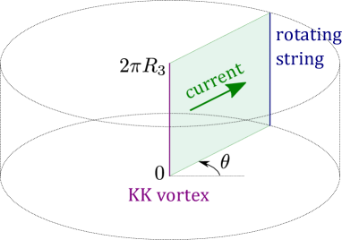
Figure 2: Outflow of the ${\rm F}1(4)$ charge from the KK vortex to the rotating probe string. The vertical direction is $x^{3}$, which has a period $2\pi R_{3}$.

The total amount of the ${\rm F}1(4)$ charge localized on the probe string at $\theta$ is

$$q_{4}(\theta)=\int_{V}*_{\rm 4E}\mathbf{j}_{4}(x)=q_{{\rm F}1}\,\frac{\theta}{2\pi}\,.$$ (2.19)

Thus, after the probe goes around the KK vortex once (i.e. $\theta=0\to 2\pi$), its ${\rm F}1(4)$ charge is increased by $q_{{\rm F}1}$, which agrees exactly with the expectation from the monodromy (1.6).

We can also describe the charge transfer process from another approach based on a collective coordinate of the KK vortex [26]. As is discussed in [29], the (unsmeared) KKM background has a zero-mode deformation associated with the $B$-field; $\delta\hat{B}^{(2)}=\beta\,\Omega_{\rm TN}$ with $\Omega_{\rm TN}$ a harmonic self-dual two form in the Taub-NUT space. After smearing, this zero-mode deformation takes the following form (see e.g. Appendix A in [30]):

$$\delta\hat{B}^{(2)}=\beta\,{\mathrm{d}}\bigl{[}H^{-1}\,\bigl{(}{\mathrm{d}}x^{4}-\sigma\,(\theta/2\pi)\,{\mathrm{d}}x^{3}\bigr{)}\bigr{]}\,.$$ (2.20)

In the following, we analyze the zero-mode excitation by promoting $\beta$ to a dynamical variable $\beta(t)$. The relevant term in the action for the background fields is

$$-\frac{1}{2\kappa_{10}^{2}}\,\int\frac{1}{2}\,\hat{H}^{(3)}\wedge*_{10}\hat{H}^{(3)} =\frac{2\pi V_{3\cdots 9}}{2\kappa_{10}^{2}}\,\int{\mathrm{d}}t\int_{0}^{r_{\infty}}\,{\mathrm{d}}r\,\frac{2\pi}{r\sigma\,[\log(r_{\rm c}/r)]^{3}}\,\dot{\beta}(t)^{2}$$

$$=\frac{\sigma V_{3\cdots 9}}{4\kappa_{10}^{2}\,H^{2}(r_{\infty})}\,\int{\mathrm{d}}t\,\dot{\beta}(t)^{2}\,,$$ (2.21)

where we have introduced an upper cutoff $r_{\infty}\,(\leq r_{\rm c})$ in the integral of radius $r$. We also have the following contribution from the action of the probe string:

$$-\frac{1}{4\pi l_{s}^{2}}\,\int{\mathrm{d}}^{2}\sigma\,{\mathrm{d}}^{4}x\,\delta^{4}(x-X(\boldsymbol{\sigma}))\,\epsilon^{ab}\,\hat{B}^{(2)}_{MN}\,\partial_{a}X^{M}\,\partial_{b}X^{N}$$

$$=\frac{\sigma R_{3}}{2\pi l_{s}^{2}}\,\int{\mathrm{d}}t\,\frac{\beta(t)}{H^{2}(X^{r})}\,\partial_{0}\bigl{[}H(X^{r})\,X^{\theta}\bigr{]}\,,$$ (2.22)

where we have chosen $X^{t}(\boldsymbol{\sigma})=\sigma^{0}$, $X^{3}(\boldsymbol{\sigma})=2\pi R_{3}\,\sigma^{1}$, $X^{r}(\boldsymbol{\sigma})$ and $X^{\theta}(\boldsymbol{\sigma})$ arbitrary but $X^{r}(\boldsymbol{\sigma})$ is large. To proceed with the analysis, we need to regularize the pathological divergence of the background at large radius. Here, we use an ad hoc procedure given in [2]; we put $H(r_{\infty})\sim 1$ and $H(X^{r})\sim 1$ as if the background is asymptotically flat. Then, the equation of motion for $\beta(t)$ becomes

$$\ddot{\beta}(t)=\frac{H^{2}(r_{\infty})}{H^{2}(X^{r})}\,\frac{\kappa_{10}^{2}}{2\pi^{2}l_{s}^{2}\,V_{4\cdots 9}}\,\partial_{0}\bigl{[}H(X^{r})\,X^{\theta}\bigr{]}\sim\frac{\kappa_{10}^{2}}{2\pi^{2}l_{s}^{2}\,V_{4\cdots 9}}\,\partial_{0}X^{\theta}\,,$$ (2.23)

and we obtain

$$\dot{\beta}(t)=\frac{2\kappa_{10}^{2}}{2\pi l_{s}^{2}\,V_{4\cdots 9}}\,\frac{X^{\theta}}{2\pi}\,.$$ (2.24)

Thus, once the probe string goes around the center ($X^{\theta}=0\to 2\pi$), $\dot{\beta}$ becomes

$$\dot{\beta}=\frac{2\kappa_{10}^{2}}{2\pi l_{s}^{2}\,V_{4\cdots 9}}\,,$$ (2.25)

and, by using this value of $\dot{\beta}$, the flux integral associated with the ${\rm F}1(4)$ charge becomes

$$\sigma_{{\rm F}1(4)}^{-1}\,\int_{\partial D}\iota_{9}\cdots\iota_{5}\iota_{3}*_{10}\hat{H}^{(3)}=-\dot{\beta}\,\frac{2\pi l_{s}^{2}\,\sigma\,V_{35\cdots 9}}{2\kappa_{10}^{2}\,H(r_{\infty})}\sim-1\,,$$ (2.26)

where $\partial D$ is a circle with the radius $r_{\infty}$, $\iota_{i}$ is the interior product of the coordinate basis $\partial_{i}$ with differential forms, and $\sigma_{{\rm F}1(4)}$ is a parameter defined in (C.4) (see Appendix C for the Page charges of defect branes). That is, just a unit of ${\rm F}1(4)$ charge is transferred from the background to the probe string during the process. Repeating the process arbitrary times, we can obtain a background with arbitrary number of ${\rm F}1(4)$ charges.

In section 4, we explicitly construct a KK-vortex solution which has the same $H$-flux with that obtained from the $B$-field (2.20) (with $\dot{\beta}=\text{const.}$). Before that, in the next section, we review the notions of Alice string and Cheshire charge, which play important roles in the discussion of the charge conservation law.

3 Alice string and defect brane

In this section, we first give a detailed review of the notions of Alice string and Cheshire charge, which appear in a certain type of $(1+3)$-dimensional gauge theories. We then argue that defect branes in string theory can be regarded as Alice strings and discuss the charge changing process in the KK-vortex background from this point of view.

3.1 Alice string and Cheshire charge

Alice strings [7] and Cheshire charges [8, 9] appear in $(1+3)$-dimensional gauge theories where a charge conjugation is a gauge symmetry of the theories. For clearness, we explain Alice strings and Cheshire charges by using one of the simplest models which admits Alice strings [7, 8, 31]. Consider a $(1+3)$-dimensional gauge theory with gauge symmetry $G=SO(3)$ and a scalar field in the $5$-dimensional representation, which we denote as a real symmetric traceless $3\times 3$ matrix $\Phi_{ij}(x)$. By choosing a quartic potential $V(\Phi)$ with appropriate coefficients, the classical vacuum configuration is given by

$$\langle\Phi\rangle=\Phi_{0}\equiv\begin{pmatrix}\,v\,&0&0\\ 0&\,v\,&0\\ 0&0&-2v\end{pmatrix}\,,$$ (3.1)

in a certain gauge. If we denote the generators of $G=SO(3)$ as $(t_{k})_{ij}=-{\hskip 0.7pt\mathrm{i}\hskip 0.7pt}\epsilon_{ijk}$ ($i,j,k=1,2,3$), the unbroken gauge symmetry (which keeps the vacuum configuration $\Phi_{0}$ invariant) is a subgroup $H=U(1)\rtimes{\mathbb{Z}}_{2}$, where the $U(1)$ transformation is generated by $Q_{0}\equiv t_{3}$ and the ${\mathbb{Z}}_{2}$ transformation is generated by

$$X\equiv\operatorname{e}^{\,{\hskip 0.7pt\mathrm{i}\hskip 0.7pt}\pi\,t_{1}}=\begin{pmatrix}\,1\,&0&0\\ 0&-1&0\\ 0&0&-1\end{pmatrix}\,.$$ (3.2)

Since $Q_{0}$ and $X$ satisfies $X\,Q_{0}\,X^{-1}=-Q_{0}$, $X$ corresponds to charge conjugation associated with the unbroken $U(1)$ gauge symmetry.

In this model, an Alice string solution can be constructed as follows. In order to make the energy of the configuration finite, we first impose $D_{\mu}\Phi=0$ at spatial infinity where $D_{\mu}$ is a covariant derivative associated with the $SO(3)$ gauge field. This condition is satisfied with

$$\Phi(\theta)\equiv\lim_{r\to\infty}\Phi(r,\theta) =U(\theta)\,\Phi_{0}\,U^{-1}(\theta)\,,\quad U(\theta)\equiv\mathrm{P}\operatorname{e}^{\,{\hskip 0.7pt\mathrm{i}\hskip 0.7pt}\int_{0}^{\theta}{\mathrm{d}}\theta\,A_{\theta}}\rvert_{r\to\infty}\,,$$ (3.3)

where we have set $\Phi(\theta=0)=\Phi_{0}$ and $(r,\,\theta)$ are polar coordinates in the two-dimensional space transverse to the string. Secondly, we impose the condition that $U(\theta=2\pi)$ be in the disconnected part of the gauge group;

$$U(\theta=2\pi)\in H_{\rm d}\,,\quad H_{\rm d}\equiv\{X\,\operatorname{e}^{\,{\hskip 0.7pt\mathrm{i}\hskip 0.7pt}\alpha\,Q_{0}}\ |\ 0\leq\alpha<2\pi\}\,.$$ (3.4)

This is the defining property of Alice strings. Concretely, we will choose $U(\theta=2\pi)=X$, which can be realized by setting $A_{\theta}\rvert_{r\to\infty}=t_{1}/2$. This leads to the following ansatz for the global behavior of an Alice string:

$$A_{\theta}=f(r)\,t_{1}/2\,,\quad\Phi(r,\theta)=\operatorname{e}^{\,{\hskip 0.7pt\mathrm{i}\hskip 0.7pt}\theta\,t_{1}/2}g(r)\,\operatorname{e}^{\,-{\hskip 0.7pt\mathrm{i}\hskip 0.7pt}\theta\,t_{1}/2}\,.$$ (3.5)

The functions $f$ and $g=(g_{ij})$ can be determined numerically from the equations of motion (see e.g. [31]) although we will not need it here.

According to the $\theta$-dependence in (3.3), the embedding of $U(1)\rtimes{\mathbb{Z}}_{2}$ into $G=SO(3)$ is non-trivially rotated around the string. Namely, if we define the unbroken subgroup of $G$ at $\theta$ by $H(\theta)\equiv\{g\in G\ |\ g\,\Phi(\theta)\,g^{-1}=\Phi(\theta)\}$, equation (3.3) leads to

$$H(\theta)=U(\theta)\,H(\theta=0)\,U^{-1}(\theta)\,.$$ (3.6)

Correspondingly, the $U(1)$ generator $Q(\theta)$ of $H(\theta)$ is related with the $U(1)$ generator $Q(\theta=0)$ of $H(\theta=0)$ as

$$Q(\theta)=U(\theta)\,Q(\theta=0)\,U^{-1}(\theta)\,.$$ (3.7)

If we set $Q(\theta=0)$ to be $Q_{0}$, for $\theta=2\pi$, we have

$$Q(\theta=2\pi)=\operatorname{e}^{\,{\hskip 0.7pt\mathrm{i}\hskip 0.7pt}\pi t_{1}}\,Q_{0}\,\operatorname{e}^{\,-{\hskip 0.7pt\mathrm{i}\hskip 0.7pt}\pi t_{1}}=X\,Q_{0}\,X=-Q_{0}\,.$$ (3.8)

That is, the sign of the $U(1)$ generator becomes opposite as one goes around the string once. This property is the reason why the vortex is called an Alice string; the monodromy works as a “charge-conjugation looking glass” [7, 32]. Since $Q(\theta=4\pi)=Q_{0}$, the $U(1)$ generator is double-valued in the transverse two-dimensional space.

In the presence of Alice strings, the electrodynamics associated with the unbroken $U(1)$ gauge group is called Alice electrodynamics. It is locally similar to the usual electrodynamics but has a strange phenomenon; when a charged particle goes around the Alice string once, the sign of the charge flips like $q\to-q$ due to property (3.8). Apparently this phenomenon seems to be in conflict with the charge conservation law.

In order to discuss the charge conservation in the Alice string background more precisely, we need to explain another issue closely related with the charge flipping phenomenon. In the presence of a single Alice string, the electric field is double-valued due to the double-valuedness (3.8) of the $U(1)$ generator. If we introduce a branch cut on a half line, $\theta=0$ (see Figure 3), and consider two branches which are glued together at the cut, the property (3.8) means that the electric fields on two branches have opposite signs.

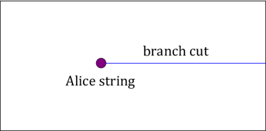
Figure 3: A branch cut on the cross-sectional plane of an Alice string.

Thus, the flux integral on a large surface is not well-defined, and we cannot define the total charge in the system.

In contrast to an isolated string, we can define a total charge for a pair of an Alice string and an anti-Alice string (see Figure 4).

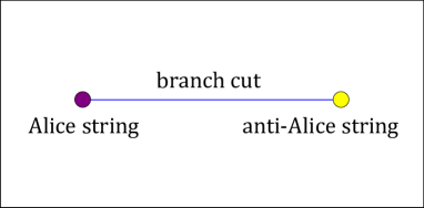
Figure 4: The cross-sectional plane of a pair of Alice and anti-Alice sting. The segment between the two strings is taken as a branch cut.

In this case, as we go around a circle which encloses the pair of strings, the $U(1)$ generator comes back to the original value since the (untraced) Wilson loop $U(2\pi)$ associated with the Alice string is canceled by that associated with the anti-Alice string. Namely, an asymptotic observer who never crosses the branch cut is always sitting on one side of the branch, and we can unambiguously define the total electric charge as an integral of the electric flux on the branch.

Before we proceed further, we should comment on the definition of the electric field. For convenience, we take a unitary gauge in which the asymptotic value of the scalar field becomes constant except for on the branch cut; $\Phi=\Phi_{0}$. In this (singular) gauge, the flipping of $U(1)$ generator occurs just above the branch cut. Then, the charge of a particle is invariant as long as it does not cross the cut, and its charge is flipped discontinuously only when it crosses the cut. We can then define the electric field at a point $x$ by measuring the force at $x$ felt by a test particle with charge $+q$ which is taken from an asymptotic region without crossing the branch cut. According to this definition, the electric field must change its sign at the branch cut since the force felt by the test particle should not change discontinuously.

Now, we can state the notion of Cheshire charge. A Cheshire charge is a charge without localized source that appears when a charged particle goes around the Alice string. In Figure 5, we sketched how such a charge can appear in the process. In step (a) and (b), a particle with charge $+q$ is approaching the branch cut from below. In the step from (b) to (c), the particle crossed the branch cut and the charge has become $-q$. After the configuration described in (c), we take the particle to infinity without crossing the cut. The resulting configuration is drawn in (d), where there appears non-zero electric flux emanating from the branch cut. Since the branch cut is just an artifact of the singular unitary gauge, there is no localized source of the electric flux. This kind of charge (without localized source) is called a Cheshire charge. The total amount of the Cheshire charge can be obtained from a flux integral around the cut, which gives $+2q$. Thus, the charge conservation law is kept intact in the whole process.

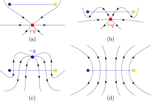
Figure 5: The process in which the Cheshire charge appears.

3.2 Defect branes as Alice strings

Here, we explain an analogy between defect branes and Alice strings, by using the KK-vortex as an example of defect branes. Then, by using the analogy, we discuss the charge transfer process in the KK-vortex background.

If we introduce the generalized metric for the KK-vortex background (1.3), it takes the following $\theta$-dependence:

$$\mathcal{H}^{-1}(\theta)=\Omega_{{\rm KKM}}^{\rm T}(\theta)\,\mathcal{H}^{-1}(\theta=0)\,\Omega_{{\rm KKM}}(\theta)\,,$$ (3.9)

$$\Omega_{{\rm KKM}}(\theta)\equiv\begin{pmatrix}{\boldsymbol{\omega}}(\theta)^{\rm T}&\mathbf{0}\cr\mathbf{0}&{\boldsymbol{\omega}}(\theta)^{-1}\cr\end{pmatrix}\,,\quad{\boldsymbol{\omega}}(\theta)\equiv\begin{pmatrix}1&0\cr\sigma\,(\theta/2\pi)&\,1\,\cr\end{pmatrix}\,.$$ (3.10)

By using the same matrix $\Omega_{{\rm KKM}}(\theta)$, the charge vector of the rotating probe string at $\theta$ can be written as [see (2.19)]

$$\vec{q}(\theta)\equiv\footnotesize\begin{pmatrix}(1/R_{3})\times\#\mathrm{P}(3)\cr(1/R_{4})\times\#\mathrm{P}(4)\cr(R_{3}/l_{s}^{2})\times\#\mathrm{F1}(3)\cr(R_{4}/l_{s}^{2})\times\#\mathrm{F1}(4)\end{pmatrix}=\footnotesize\begin{pmatrix}0\cr 0\cr(R_{3}/l_{s}^{2})\times 1\cr(R_{4}/l_{s}^{2})\times\frac{\theta}{2\pi}\end{pmatrix}=\Omega_{{\rm KKM}}^{-1}(\theta)\,\vec{q}(\theta=0)\,.$$ (3.11)

This relation is reminiscent of equation (3.7). Since the charge vector is non-trivially twisted around the center, the KK vortex (or general defect branes with non-trivial monodromies) can be regarded as Alice strings. Note that the discrete gauge symmetry ${\mathbb{Z}}_{2}$ (in the case of the above model of Alice strings) is generalized to U-duality group in the case of string theory.

As is the case with a single Alice string, we do not have a globally well-defined notion of the total winding charge in a KK-vortex background. However, in this case, it will be natural to define the “total charge” by

$$\vec{\mathbf{Q}}\equiv\sum_{i}\Omega_{{\rm KKM}}(\theta_{i})\,\vec{q}_{i}\qquad(-\infty<\theta_{i}<\infty)\,,$$ (3.12)

where $\theta_{i}$ is the value of the angular variable associated with the $i$-th particle. This definition is essentially the same as that used in [4], and, with this definition, the charge of the probe does not change. Indeed, for the case of the rotating probe string, the winding charge of a probe string at $\theta$ is given by $\vec{q}(\theta)=\Omega_{{\rm KKM}}^{-1}(\theta)\,\vec{q}(\theta=0)$ [see (3.11)] and $\Omega_{{\rm KKM}}(\theta)\,\vec{q}(\theta)$ is independent of $\theta$ ; i.e., no ${\rm F}1(4)$ charge appears. However, in the field theoretical analysis performed in section 2, the probe produces a non-zero flux (2.17) associated with the ${\rm F}1(4)$ charge during the rotation, and it will be more natural to invent a definition such that the probe charge can change in time.

We thus define the “total charge” by

$$\vec{Q}\equiv\sum_{i}\Omega_{{\rm KKM}}(\theta_{i})\,\vec{q}_{i}\qquad(0\leq\theta_{i}<2\pi)\,.$$ (3.13)

Conceptually, this definition can be realized by the following procedure. We first fix a base point on $\theta=0$ and introduce a curve which encloses all charged particles but does not cross the branch cut (see Figure 6).

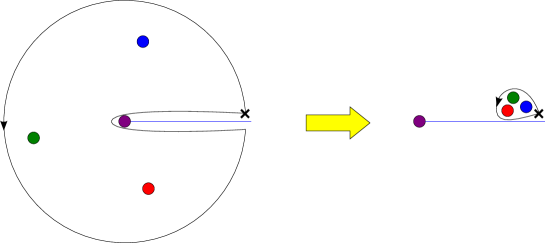
Figure 6: The conceptual procedure to define the “total charge” $\vec{Q}$.

Then, by shrinking the curve, we assemble all charged particles to the base point. Now, since all particles have the same basis for the charge vector, we can just add up the components of their charge vectors to compute the “total charge” $\vec{Q}$ . With this definition, as is the case of $\vec{\mathbf{Q}}$ , the charge remains constant during the rotation of a probe string as long as the string does not cross a branch cut. However, if the probe string crosses the branch cut, its winding charge must discretely change since the matrix discretely jump from $\Omega_{{\rm KKM}}(2\pi)$ to $\Omega_{{\rm KKM}}(0)$ ;

$$\vec{Q}=\Omega_{{\rm KKM}}(2\pi-0)\,\footnotesize\begin{pmatrix}0\cr 0\cr(R_{3}/l_{s}^{2})\times 1\cr(R_{4}/l_{s}^{2})\times\frac{2\pi-0}{2\pi}\end{pmatrix}=\footnotesize\begin{pmatrix}0\cr 0\cr(R_{3}/l_{s}^{2})\times 1\cr 0\end{pmatrix}$$

$$\to\quad \vec{Q}=\Omega_{{\rm KKM}}(+0)\,\footnotesize\begin{pmatrix}0\cr 0\cr(R_{3}/l_{s}^{2})\times 1\cr(R_{4}/l_{s}^{2})\times\frac{2\pi+0}{2\pi}\end{pmatrix}=\footnotesize\begin{pmatrix}0\cr 0\cr(R_{3}/l_{s}^{2})\times 1\cr(R_{4}/l_{s}^{2})\times 1\end{pmatrix}\,.$$ (3.14)

That is, if we adopt the definition, the situation is similar to the case where the singular unitary gauge is taken in the presence of Alice strings, and the discrete change of the probe charge should be compensated by the Cheshire charge, which corresponds to the zero-mode deformation associated with the $B$-field.

Geometrically, the discrete jump (3.14) when a probe crossed the branch cut can be realized as a change of coordinates given by (1.7). This is the reason why we did not use the original coordinate $(x^{3},\,x^{4})$ but used $(x^{\prime 3},\,x^{\prime 4})$ to calculate the winding number in the introduction. For more general cases where there are multiple probe strings, it will be more effective to perform an active diffeomorphism

$$x^{\prime 3}=x^{3}\,,\qquad x^{\prime 4}=x^{4}+\sigma\,x^{3}\,,$$ (3.15)

when a probe string crosses the branch cut, although the winding number is always measured with the use of the original coordinates.

4 Kaluza-Klein dyon and dyonic Kaluza-Klein vortex

In this section, we first review the construction of the KK-dyon solution in four-dimensional theory [27]. We point out that, if we uplift the solution to ten dimensions, the background has ${\rm F}1(4)$ charges although there is no localized source, just like Cheshire charges. We then construct a KK-vortex solution with an arbitrary number of ${\rm F}1(4)$ Cheshire charges, which we call a dyonic KK vortex, and discuss the relation to the charge transfer process considered in section 2.

4.1 Kaluza-Klein dyon

The KK-monopole solution in ten-dimensional spacetime is given by

$${\mathrm{d}}s^{2} =-{\mathrm{d}}t^{2}+H(r)\,\bigl{(}{\mathrm{d}}r^{2}+r^{2}\,{\mathrm{d}}\Omega_{2}^{2}\bigr{)}+H^{-1}(r)\,\bigl{(}{\mathrm{d}}x^{4}+\omega\bigr{)}^{2}+{\mathrm{d}}x^{2}_{56789}\,,$$ (4.1)

$$\operatorname{e}^{\,2\hat{\phi}} =1\,,\quad\hat{B}^{(2)}=0\,,\quad H(r)\equiv 1+\frac{R_{4}}{2\,r}\,,\quad{\mathrm{d}}\Omega_{2}^{2}\equiv{\mathrm{d}}\theta^{2}+\sin^{2}\theta\,{\mathrm{d}}\varphi^{2}\,,$$ (4.2)

where $R_{4}$ is the radius of the $x^{4}$-direction and $\omega$ satisfies ${\mathrm{d}}\omega=\hat{*}_{3}\,{\mathrm{d}}H(r)$ ($\hat{*}_{3}$: Hodge star operator in a flat three-dimensional space), which can be solved by

$$\omega=-\frac{R_{4}}{2}\,(1-\cos\theta)\,{\mathrm{d}}\varphi\,.$$ (4.3)

Compactifying on the six-torus $T^{6}_{4\cdots 9}$ (spanned by $x^{4}\,,\dotsc,\,x^{9}$), we obtain the four-dimensional configuration:

$$\lambda \equiv\chi+{\hskip 0.7pt\mathrm{i}\hskip 0.7pt}\operatorname{e}^{\,-2\phi}={\hskip 0.7pt\mathrm{i}\hskip 0.7pt}\,H^{-1/2}(r)\,,$$ (4.4)

$${\mathrm{d}}s_{\rm 4E}^{2} =\operatorname{e}^{\,-2\phi}{\mathrm{d}}s_{4}^{2}=-H^{-1/2}(r)\,{\mathrm{d}}t^{2}+H^{1/2}(r)\,\bigl{(}{\mathrm{d}}r^{2}+r^{2}\,{\mathrm{d}}\Omega_{2}^{2}\bigr{)}\,,$$ (4.5)

$$\begin{pmatrix}\mathcal{F}^{4}\cr\mathcal{F}_{4}\end{pmatrix} =\begin{pmatrix}{\mathrm{d}}\mathcal{A}^{4}\cr{\mathrm{d}}\mathcal{A}_{4}\end{pmatrix}\,,\qquad\begin{pmatrix}\mathcal{A}^{4}\cr\mathcal{A}_{4}\end{pmatrix}=\begin{pmatrix}\omega\cr 0\end{pmatrix}\,.$$ (4.6)

Here, ${\mathrm{d}}s_{\rm 4E}^{2}$ is the line element in the four-dimensional Einstein frame while ${\mathrm{d}}s_{4}^{2}$ is that in the string frame.

Now, we make a replacement $R_{4}\to\Delta^{1/2}\,R_{4}$ in the metric and $H(r)$, and use the $SL(2,{\mathbb{R}})$ duality in four dimensions (see Appendix B) to obtain the following KK-dyon solution [27]:

$${\mathrm{d}}s_{\rm 4E}^{2} =-H^{-1/2}(r)\,{\mathrm{d}}t^{2}+H^{1/2}(r)\,\bigl{(}{\mathrm{d}}r^{2}+r^{2}\,{\mathrm{d}}\Omega_{2}^{2}\bigr{)}\,,$$ (4.7)

$$\lambda =\chi+{\hskip 0.7pt\mathrm{i}\hskip 0.7pt}\operatorname{e}^{\,-2\phi}=\frac{\mathsf{a}\,\mathsf{c}+\mathsf{b}\,\mathsf{d}\,H(r)}{\mathsf{c}^{2}+\mathsf{d}^{2}\,H(r)}+{\hskip 0.7pt\mathrm{i}\hskip 0.7pt}\,\frac{H^{1/2}(r)}{\mathsf{c}^{2}+\mathsf{d}^{2}\,H(r)}\,,$$ (4.8)

$$\begin{pmatrix}\mathcal{F}^{4}\cr\mathcal{F}_{4}\end{pmatrix} =\begin{pmatrix}{\mathrm{d}}\mathcal{A}^{4}\cr{\mathrm{d}}\mathcal{A}_{4}\end{pmatrix}\,,\qquad\begin{pmatrix}\mathcal{A}^{4}\cr\mathcal{A}_{4}\end{pmatrix}=\begin{pmatrix}\mathsf{d}\,\omega\cr\frac{\mathsf{c}}{H(r)}\,{\mathrm{d}}t\end{pmatrix}\,.$$ (4.9)

We use the following parameterization of the $SL(2,{\mathbb{R}})$ matrix [27]:

$$\begin{pmatrix}\mathsf{a}&\mathsf{b}\cr\mathsf{c}&\mathsf{d}\end{pmatrix}=\begin{pmatrix}\,\chi_{0}\,\operatorname{e}^{\,\phi_{0}}\sin\alpha+\operatorname{e}^{\,-\phi_{0}}\cos\alpha\,&\,\chi_{0}\,\operatorname{e}^{\,\phi_{0}}\cos\alpha-\operatorname{e}^{\,-\phi_{0}}\sin\alpha\,\cr\operatorname{e}^{\,\phi_{0}}\sin\alpha&\operatorname{e}^{\,\phi_{0}}\cos\alpha\end{pmatrix}\,,$$ (4.10)

where $\phi_{0}$, $\chi_{0}$ and $\alpha$ are real free parameters to be fixed below. Under this $SL(2,{\mathbb{R}})$ transformation, the charge vector transforms as [see (B.21) and (B.22)]

$$\footnotesize\begin{pmatrix}p^{4}\cr p_{4}\cr q^{4}\cr q_{4}\end{pmatrix}=\begin{pmatrix}\mathsf{d}\,\mathbf{1}&-\mathsf{c}\,L\cr-\mathsf{b}\,L&\mathsf{a}\,\mathbf{1}\end{pmatrix}\footnotesize\begin{pmatrix}\Delta^{1/2}\,q_{{\rm KKM}}\cr 0\cr 0\cr 0\end{pmatrix}=\footnotesize\begin{pmatrix}\mathsf{d}\,\Delta^{1/2}\,q_{{\rm KKM}}\cr 0\cr 0\cr-\mathsf{b}\,\Delta^{1/2}\,\gamma\,q_{{\rm F}1}\end{pmatrix}$$ (4.11)

with $L=\bigl{(}\begin{smallmatrix}0&1\cr 1&0\end{smallmatrix}\bigr{)}$ and $\gamma\equiv q_{{\rm KKM}}/q_{{\rm F}1}=g_{s}^{-2}\,V_{4\cdots 9}/(2\pi l_{s})^{6}$ . We require that each component of the charge vector is an integral multiple of the elementary charge:

$$\mathsf{d}\,\Delta^{1/2}\equiv P\in{\mathbb{Z}}\qquad\text{and}\qquad\mathsf{b}\,\Delta^{1/2}\,\gamma\equiv Q\in{\mathbb{Z}}\,.$$ (4.12)

Using the integers $P$ and $Q$, the $SL(2,{\mathbb{R}})$ matrix can be written as

$$\begin{pmatrix}\mathsf{a}&\mathsf{b}\cr\mathsf{c}&\mathsf{d}\end{pmatrix} =\begin{pmatrix}\frac{\gamma\,P-\chi_{0}\,(Q-\chi_{0}\,\gamma\,P)}{\Delta^{1/2}\,\gamma}&\frac{Q}{\Delta^{1/2}\,\gamma}\cr-\frac{Q-\chi_{0}\,\gamma\,P}{\Delta^{1/2}\,\gamma}&\frac{P}{\Delta^{1/2}}\end{pmatrix}\,,$$ (4.13)

$$\Delta^{1/2} =\sqrt{P^{2}+\gamma^{-2}\,(Q-\chi_{0}\,\gamma\,P)^{2}}\,,$$ (4.14)

where we have set $\phi_{0}=0$ since the $\phi_{0}$ dependence can be absorbed into a redefinition of coordinates and the ten-dimensional dilaton.

From the above solution, we can reconstruct the ten-dimensional solution:

$${\mathrm{d}}s^{2} =-\frac{\mathsf{c}^{2}+\mathsf{d}^{2}\,H(r)}{H(r)}\,{\mathrm{d}}t^{2}+\bigl{[}\mathsf{c}^{2}+\mathsf{d}^{2}\,H(r)\bigr{]}\,\bigl{(}{\mathrm{d}}r^{2}+r^{2}\,{\mathrm{d}}\Omega_{2}^{2}\bigr{)}$$

$$\quad+H^{-1}(r)\,\bigl{(}{\mathrm{d}}x^{4}+\mathsf{d}\,\omega\bigr{)}^{2}+{\mathrm{d}}x^{2}_{56789}\,,$$ (4.15)

$$\operatorname{e}^{\,2\hat{\phi}} =\frac{\mathsf{c}^{2}+\mathsf{d}^{2}\,H(r)}{H(r)}\,,\quad\hat{B}^{(2)}=\frac{\mathsf{c}}{H(r)}\,{\mathrm{d}}t\wedge\bigl{(}{\mathrm{d}}x^{4}+\mathsf{d}\,\omega\bigr{)}\,,$$ (4.16)

$$\hat{H}^{(3)} =-\mathsf{c}\,{\mathrm{d}}t\wedge{\mathrm{d}}\Bigl{[}\frac{1}{H(r)}\,\bigl{(}{\mathrm{d}}x^{4}+\mathsf{d}\,\omega\bigr{)}\Bigr{]}\,.$$ (4.17)

As the charge vector (4.11) indicates, this background includes $P$ KK-monopoles as well as $(-Q)$ F1(4) charge. The flux integral associated with F1(4) charge is calculated as

$$\frac{1}{2\kappa^{2}_{10}}\,\int_{S^{2}_{\infty}\times T^{5}_{5\cdots 9}}\operatorname{e}^{\,-2\hat{\phi}}\,*_{10}\hat{H}^{(3)}=-\mu_{{\rm F}1}\,\bigl{(}Q-\chi_{0}\,\gamma\,P\bigr{)}\qquad\Bigl{(}\mu_{{\rm F}1}\equiv\frac{1}{2\pi l_{s}^{2}}\Bigr{)}\,,$$ (4.18)

where we have used $\mathsf{c}^{2}+\mathsf{d}^{2}=1$, $\mathsf{c}\,\Delta^{1/2}=-\gamma^{-1}\,(Q-\chi_{0}\,\gamma\,P)$, and

$$\operatorname{e}^{\,-2\hat{\phi}}\,*_{10}\hat{H}^{(3)}$$

$$=\left\{\begin{array}[]{ll}{\mathrm{d}}\Bigl{[}\frac{\mathsf{c}/\mathsf{d}}{\mathsf{c}^{2}+\mathsf{d}^{2}\,H(r)}\,\Bigl{(}{\mathrm{d}}x^{4}+\frac{\mathsf{d}\,\Delta^{1/2}\,R_{4}}{2}\,(1-\cos\theta)\,{\mathrm{d}}\varphi\Bigr{)}\Bigr{]}\wedge{\mathrm{d}}x^{5}\wedge\cdots\wedge{\mathrm{d}}x^{9}&(\mathsf{d}\neq 0)\,,\cr\frac{R_{4}\,\Delta^{1/2}}{2}\,\sin\theta\,{\mathrm{d}}\theta\wedge{\mathrm{d}}\varphi\wedge{\mathrm{d}}x^{5}\wedge\cdots\wedge{\mathrm{d}}x^{9}&(\mathsf{d}=0)\,.\end{array}\right.$$ (4.21)

In the case of $\mathsf{d}\neq 0$, the flux integral over a sphere with the radius $r_{0}$ ($\times T^{5}_{56789}$) gives

$$Q_{{\rm F}1(4)}^{0}\equiv-\mu_{{\rm F}1}\,\frac{Q-\chi_{0}\,\gamma\,P}{\mathsf{c}^{2}+\mathsf{d}^{2}\,H(r_{0})}\,.$$ (4.22)

Since the flux integral increases monotonically from $0$ to $-\mu_{{\rm F}1}\,\bigl{(}Q-\chi_{0}\,\gamma\,P\bigr{)}$ as we vary $r_{0}$ from $0$ to $\infty$, we may conclude that the F1 charge is distributed over the non-compact three-dimensional space except the origin, $r=0$. However, if we consider a flux integral over an arbitrary closed surface which does not enclose the origin, the integral gives zero. Thus, it does not make sense to consider the local distribution of the source. We can just associate the F1 charges to a non-trivial cycle $S^{2}_{\infty}$, as in the case of the Cheshire charge.

4.2 Dyonic Kaluza-Klein vortex

Here, we first construct the dyonic KK-vortex solution, and compute the charges both in the four-dimensional viewpoint and in the ten-dimensional viewpoint. It turns out that the background has F1(4) Cheshire charges. We will then relate the background with the charge transfer process considered in section 2.

By smearing the Kaluza-Klein dyon along the $x^{3}$-direction, we obtain the following background (see e.g. [2, 18] for the smearing procedure):

$${\mathrm{d}}s^{2} =-\frac{\mathsf{c}^{2}+\mathsf{d}^{2}\,H(r)}{H(r)}\,{\mathrm{d}}t^{2}+\bigl{[}\mathsf{c}^{2}+\mathsf{d}^{2}\,H(r)\bigr{]}\,\bigl{(}{\mathrm{d}}r^{2}+r^{2}\,{\mathrm{d}}\theta^{2}+{\mathrm{d}}x_{3}^{2}\bigr{)}$$

$$\quad+H^{-1}(r)\,\bigl{(}{\mathrm{d}}x^{4}+\mathsf{d}\,\omega\bigr{)}^{2}+{\mathrm{d}}x^{2}_{56789}\,,$$ (4.23)

$$\operatorname{e}^{\,2\hat{\phi}} =\frac{\mathsf{c}^{2}+\mathsf{d}^{2}\,H(r)}{H(r)}\,,\qquad\hat{B}^{(2)}=\frac{\mathsf{c}}{H(r)}\,{\mathrm{d}}t\wedge\bigl{(}{\mathrm{d}}x^{4}+\mathsf{d}\,\omega\bigr{)}\,,$$ (4.24)

$$\hat{H}^{(3)} =-\mathsf{c}\,{\mathrm{d}}t\wedge{\mathrm{d}}\Bigl{[}\frac{1}{H(r)}\,\bigl{(}{\mathrm{d}}x^{4}+\mathsf{d}\,\omega\bigr{)}\Bigr{]}\,,$$ (4.25)

where $H(r)=(\bar{\sigma}/2\pi)\,\log(r_{\rm c}/r)$, $\bar{\sigma}\equiv\sigma\,\Delta^{1/2}=(R_{4}/R_{3})\,\Delta^{1/2}$, and $\omega=-\bar{\sigma}\,(\theta/2\pi)\,{\mathrm{d}}x^{3}$, which satisfies ${\mathrm{d}}\omega=\hat{*}_{3}{\mathrm{d}}H(r)$.

The above background is a special case of the following general background with $\rho(z)={\hskip 0.7pt\mathrm{i}\hskip 0.7pt}(\bar{\sigma}/2\pi)\,\log(r_{\rm c}/z)=H(r)+{\hskip 0.7pt\mathrm{i}\hskip 0.7pt}(\bar{\sigma}\,\theta/2\pi)$ and $f(z)=1$ ($z\equiv r\operatorname{e}^{\,{\hskip 0.7pt\mathrm{i}\hskip 0.7pt}\theta}$) :

$${\mathrm{d}}s^{2} =\bigl{(}\mathsf{c}^{2}+\mathsf{d}^{2}\,\rho_{2}\bigr{)}\,\bigl{[}-\rho_{2}^{-1}\,{\mathrm{d}}t^{2}+{\lvert f(z)\rvert}^{2}\,{\mathrm{d}}z^{2}+{\mathrm{d}}x_{3}^{2}\bigr{]}$$

$$\quad+\rho_{2}^{-1}\,\bigl{(}{\mathrm{d}}x^{4}-\mathsf{d}\,\rho_{1}\,{\mathrm{d}}x^{3}\bigr{)}^{2}+{\mathrm{d}}x^{2}_{56789}\,,$$ (4.26)

$$\operatorname{e}^{\,2\hat{\phi}} =\frac{\mathsf{c}^{2}+\mathsf{d}^{2}\,\rho_{2}}{\rho_{2}}\,,\qquad\hat{B}^{(2)}=\frac{\mathsf{c}}{\rho_{2}}\,{\mathrm{d}}t\wedge\bigl{(}{\mathrm{d}}x^{4}-\mathsf{d}\,\rho_{1}\,{\mathrm{d}}x^{3}\bigr{)}\,.$$ (4.27)

This satisfies the equations of motion as long as $f(z)$ and $\rho(z)\equiv\rho_{1}+{\hskip 0.7pt\mathrm{i}\hskip 0.7pt}\rho_{2}$ are holomorphic functions.

Charges calculated in four-dimensional viewpoint

By compactifying on the six-torus $T^{6}_{4\cdots 9}$, we obtain the following four-dimensional configuration:

$${\mathrm{d}}s_{\rm 4E}^{2}=-\rho_{2}^{-1/2}\,{\mathrm{d}}t^{2}+\rho_{2}^{1/2}\,\bigl{(}{\lvert f\rvert}^{2}\,{\mathrm{d}}z\,{\mathrm{d}}\bar{z}+{\mathrm{d}}x_{3}^{2}\bigr{)}\,,$$ (4.28)

$$M=\begin{pmatrix}\,\rho_{2}\,&0\cr 0&\rho_{2}^{-1}\end{pmatrix}\,,\quad\lambda=\chi+{\hskip 0.7pt\mathrm{i}\hskip 0.7pt}\operatorname{e}^{\,-2\phi}=\frac{\mathsf{a}\,\mathsf{c}+\mathsf{b}\,\mathsf{d}\,\rho_{2}}{\mathsf{c}^{2}+\mathsf{d}^{2}\,\rho_{2}}+{\hskip 0.7pt\mathrm{i}\hskip 0.7pt}\frac{\rho_{2}^{1/2}}{\mathsf{c}^{2}+\mathsf{d}^{2}\,\rho_{2}}\,,$$ (4.29)

$$\begin{pmatrix}\mathcal{F}^{4}\cr\mathcal{F}_{4}\end{pmatrix}=\begin{pmatrix}{\mathrm{d}}\bigl{(}-\mathsf{d}\,\rho_{1}\,{\mathrm{d}}x^{3}\bigr{)}\cr{\mathrm{d}}\bigl{(}\frac{\mathsf{c}\,{\mathrm{d}}t}{\rho_{2}}\bigr{)}\end{pmatrix}\,,\quad\begin{pmatrix}\mathcal{G}^{4}\cr\mathcal{G}_{4}\end{pmatrix}=\begin{pmatrix}{\mathrm{d}}\bigl{(}\frac{-\mathsf{a}\,{\mathrm{d}}t}{\rho_{2}}\bigr{)}\cr{\mathrm{d}}\bigl{(}\mathsf{b}\,\rho_{1}\,{\mathrm{d}}x^{3}\bigr{)}\end{pmatrix}\,.$$ (4.30)

The duality covariant charge vector is given by

$$\vec{Q}=\footnotesize\begin{pmatrix}p^{4}\cr p_{4}\cr q^{4}\cr q_{4}\end{pmatrix} =\footnotesize\begin{pmatrix}\frac{\mathsf{d}\,(2\pi R_{3})}{2\kappa_{4}^{2}}\,\int_{C}{\mathrm{d}}\rho_{1}\cr 0\cr 0\cr-\frac{\mathsf{b}\,(2\pi R_{3})}{2\kappa_{4}^{2}}\,\int_{C}{\mathrm{d}}\rho_{1}\end{pmatrix}=\footnotesize\begin{pmatrix}P\,q_{{\rm KKM}}\cr 0\cr 0\cr-Q\,q_{{\rm F}1}\end{pmatrix}\,,$$ (4.31)

where $C$ is an arbitrary closed curve on the $z$-plane which encloses the origin $z=0$ once, and we used $\int_{C}{\mathrm{d}}\rho_{1}=\bar{\sigma}$, which follows from the choice $\rho={\hskip 0.7pt\mathrm{i}\hskip 0.7pt}(\bar{\sigma}/2\pi)\,\log(r_{\rm c}/z)$. Thus the background contains $P$ KKM(56789,4) and $(-Q)$ F1(4) charges.

On the other hand, the physical electric charge is calculated as

$$\begin{pmatrix}Q^{4}\cr Q_{4}\end{pmatrix} \equiv\frac{1}{2\kappa_{4}^{2}}\,\begin{pmatrix}\int_{C_{0}\times S^{1}}\operatorname{e}^{\,-2\phi}\,(M^{-1})^{44}\,*_{\rm 4E}\mathcal{F}_{4}\cr\int_{C_{0}\times S^{1}}\operatorname{e}^{\,-2\phi}\,(M^{-1})_{44}\,*_{\rm 4E}\mathcal{F}^{4}\end{pmatrix}=\begin{pmatrix}0\cr\frac{1}{2\kappa_{4}^{2}}\,\int_{C_{0}\times S^{1}}\frac{\mathsf{c}\,\bar{\sigma}\,{\mathrm{d}}(\theta/2\pi)\wedge{\mathrm{d}}x^{3}}{\mathsf{c}^{2}+\mathsf{d}^{2}\,\rho_{2}}\end{pmatrix}$$

$$=\begin{pmatrix}0\cr-q_{{\rm F}1}\,\frac{Q-\chi_{0}\,\gamma\,P}{\mathsf{c}^{2}+\mathsf{d}^{2}\,H(r_{0})}\end{pmatrix}\,.$$ (4.32)

where $C_{0}$ is a circle with the radius $r_{0}$ and $S^{1}$ is a circle in the $x^{3}$-direction, and we used $\rho(z)={\hskip 0.7pt\mathrm{i}\hskip 0.7pt}(\bar{\sigma}/2\pi)\,\log(r_{\rm c}/z)$. The dependence on the radius $r_{0}$ means that the charge is distributed over the branch cut (although the position of the branch cut is not physical). If we take the limit of taking $r_{0}$ large and assume that $H(r_{0})\to 1$ in the limit as in section 2, the physical electric charge then becomes $Q_{4}=-q_{{\rm F}1}\,(Q-\chi_{0}\,\gamma\,P)$ .

Charges calculated in ten-dimensional viewpoint

In the ten-dimensional viewpoint, the KKM(56789,4) charge is given by

$$Q_{{\rm KKM}(56789,4)} =-\sigma_{{\rm KKM}(56789,4)}^{-1}\,\int_{C}{\mathrm{d}}\Bigl{(}\frac{\hat{G}_{43}}{\hat{G}_{44}}\Bigr{)}=P\,,$$ (4.33)

where we used $\int_{C}{\mathrm{d}}\rho_{1}=\bar{\sigma}_{{\rm KKM}(56789,4)}$ . On the other hand, by using

$$\operatorname{e}^{\,-2\hat{\phi}}*_{10}{\mathrm{d}}\hat{H}^{(3)}={\mathrm{d}}\biggl{[}\frac{\mathsf{c}^{2}\,\rho_{1}\,{\mathrm{d}}x^{3}+\mathsf{d}\,\rho_{2}\,{\mathrm{d}}x^{4}}{\mathsf{c}\,(\mathsf{c}^{2}+\mathsf{d}^{2}\,\rho_{2})}\biggr{]}\wedge{\mathrm{d}}x^{5}\wedge\cdots\wedge{\mathrm{d}}x^{9}\,,$$ (4.34)

we can calculate the ${\rm F}1(4)$ charge as

$$\sigma_{{\rm F}1(4)}^{-1}\,\int_{C}\iota_{9}\cdots\iota_{5}\iota_{3}\operatorname{e}^{\,-2\hat{\phi}}*_{10}\hat{H}^{(3)}=-\frac{Q-\chi_{0}\,\gamma\,P}{\mathsf{c}^{2}+\mathsf{d}^{2}\,H(r_{0})}\,,$$ (4.35)

where $C$ is an arbitrary curve which encloses the origin once counterclockwise and crosses the branch cut at $r=r_{0}$. This expression coincides with the physical electric charge in four dimensions.

Although we can also compute the local distribution of the charges on the branch cut, the position of the branch cut is unphysical, and so is the local charge distribution. Thus, we can just conclude that the branch cut emanating from the KK vortex, in total, has $-(Q-\chi_{0}\,\gamma\,P)$ unit of ${\rm F}1(4)$ charge. In the following, we call this kind of charges without localized source Cheshire charges. That is, the dyonic KK-vortex background has $-(Q-\chi_{0}\,\gamma\,P)$ ${\rm F}1(4)$ Cheshire charges.

Finally, we argue that the dyonic KK-vortex solution can be regarded as a resultant background after a string goes around the vortex. To see this, we first note that the $H$-flux given in (4.25) is the same as that obtained from the $B$-field (2.20) with $\beta(t)=-\mathsf{c}\,\Delta^{1/2}\,t$ . In section 2, we considered the case of a single KK vortex (i.e. $P=1$). In order to relate the dyonic KK-vortex background with the KK-vortex background with non-zero $B$-field (considered in section 2), (2.24) indicates that we should choose $-\mathsf{c}\,\Delta^{1/2}=\mu_{{\rm F}1}\,(2\kappa_{10}^{2}/V_{4\cdots 9})\,Q$, i.e., $\chi_{0}=0$. Thus, we will set $P=1$ and $\chi_{0}=0$, which makes $\mathsf{c}=-Q/(\Delta^{1/2}\,\gamma)$, $\mathsf{d}=\Delta^{-1/2}$, and $\Delta^{1/2}=\sqrt{1+\gamma^{-2}\,Q^{2}}$ . With the above choice of parameters, we can interpret the dyonic KK-vortex background as a resultant geometry after the charge transfer process.

Energy

Before closing this section, we make a brief comment on the mass of the dyonic KK vortex. The mass can generally be computed by the following formula,

$$m=\frac{1}{2\kappa_{3}^{2}}\,\int{\mathrm{d}}^{2}x\sqrt{\gamma}\,R(\gamma)\,,$$ (4.36)

where $\gamma$ is the transverse two-dimensional metric and $2\kappa_{3}^{2}\equiv 2\kappa_{10}^{2}/V_{3\cdots 9}$. In the three-dimensional Einstein frame, the dyonic KK-vortex solution has the following metric:

$${\mathrm{d}}s^{2}=-{\mathrm{d}}t^{2}+\rho_{2}\,{\lvert f(z)\rvert}^{2}\,{\mathrm{d}}z\,{\mathrm{d}}\bar{z}\,.$$ (4.37)

Since the dyonic deformation parameters do not appear here, the mass of the dyonic KK vortex is the same as that of the non-dyonic KK vortex.

5 $5^{2}_{2}$ background with F1 Cheshire charge

If we take a $T$-duality along the $x^{3}$-direction in the dyonic KK-vortex background, we obtain the following background:

$${\mathrm{d}}s^{2} =(\mathsf{c}^{2}+\mathsf{d}^{2}\,\rho_{2})\,\bigl{(}-\rho_{2}^{-1}\,{\mathrm{d}}t^{2}+{\lvert f\rvert}^{2}\,{\mathrm{d}}z\,{\mathrm{d}}\bar{z}\bigr{)}$$

$$\quad+\frac{\rho_{2}\,\Bigl{(}{\mathrm{d}}x^{3}-\frac{\mathsf{c}\,\mathsf{d}\,\rho_{1}}{\rho_{2}}\,{\mathrm{d}}t\Bigr{)}^{2}+(\mathsf{c}^{2}+\mathsf{d}^{2}\,\rho_{2})\,{\mathrm{d}}x_{4}^{2}}{\mathsf{c}^{2}\,\rho_{2}+\mathsf{d}^{2}\,{\lvert\rho\rvert}^{2}}+{\mathrm{d}}x^{2}_{56789}\,,$$ (5.1)

$$\operatorname{e}^{\,2\hat{\phi}} =\frac{\mathsf{c}^{2}+\mathsf{d}^{2}\,\rho_{2}}{\mathsf{c}^{2}\,\rho_{2}+\mathsf{d}^{2}\,{\lvert\rho\rvert}^{2}}\,,$$ (5.2)

$$\hat{B}^{(2)} =\frac{\mathsf{c}\,(\mathsf{c}^{2}+\mathsf{d}^{2}\,\rho_{2})}{\mathsf{c}^{2}\,\rho_{2}+\mathsf{d}^{2}\,{\lvert\rho\rvert}^{2}}\,{\mathrm{d}}t\wedge{\mathrm{d}}x^{4}+\frac{\mathsf{d}\,\rho_{1}}{\mathsf{c}^{2}\,\rho_{2}+\mathsf{d}^{2}\,{\lvert\rho\rvert}^{2}}\,{\mathrm{d}}x^{3}\wedge{\mathrm{d}}x^{4}\,,$$ (5.3)

$$\hat{B}^{(6)} =\frac{\mathsf{c}\,\rho_{1}\,{\mathrm{d}}x^{3}+\mathsf{d}\,(\mathsf{c}^{2}\,\rho_{2}+\mathsf{d}^{2}\,{\lvert\rho\rvert}^{2})\,{\mathrm{d}}t}{\mathsf{c}^{2}+\mathsf{d}^{2}\,\rho_{2}}\wedge{\mathrm{d}}x^{5}\wedge\cdots\wedge{\mathrm{d}}x^{9}\,.$$ (5.4)

Here, we choose the holomorphic function as $\rho(z)={\hskip 0.7pt\mathrm{i}\hskip 0.7pt}(\bar{\sigma}_{5^{2}_{2}}/2\pi)\,\log(r_{\rm c}/z)$ with $\bar{\sigma}_{5^{2}_{2}}\equiv\Delta^{1/2}\,\sigma_{5^{2}_{2}}$ and $\sigma_{5^{2}_{2}}\equiv R_{3}\,R_{4}/l_{s}^{2}$. If we set $\mathsf{c}=0$ and $\mathsf{d}=1$, this reproduces the standard $5^{2}_{2}$-brane background [3, 2, 33]. By using the generalized metric $\mathcal{H}^{-1}$, we find the following relation:

$$\mathcal{H}^{-1}(\theta=2\pi)=\Omega_{5^{2}_{2}\text{-}{\rm F}1}^{\rm T}\,\mathcal{H}^{-1}(\theta=0)\,\Omega_{5^{2}_{2}\text{-}{\rm F}1}\,,$$ (5.5)

$$\Omega_{5^{2}_{2}\text{-}{\rm F}1}\equiv\begin{pmatrix}\mathbf{1}&\,\mathbf{0}\,\cr\mathsf{d}\,\bar{\sigma}_{5^{2}_{2}}\,\boldsymbol{\varepsilon}&\mathbf{1}\end{pmatrix}\,,\quad\boldsymbol{\varepsilon}=\begin{pmatrix}0&1\cr-1&\,0\,\end{pmatrix}\,,$$ (5.6)

which follows from the discrete shift $\rho_{1}\to\rho_{1}+\bar{\sigma}_{5^{2}_{2}}$ under the rotation $\theta=0\to 2\pi$. The monodromy matrix is exactly the same with that of the $5_{2}^{2}$ background [2], which we denote by $\Omega_{5^{2}_{2}}$, since we have chosen $\mathsf{d}\,\Delta^{1/2}=1$. Since the background fields are patched together with the use of a $T$-duality transformation, this background is a $T$-fold.

We can compute the F1(4) charge as

$$\sigma_{{\rm F}1(4)}^{-1}\,\int_{C}{\mathrm{d}}\bigl{(}\iota_{9}\cdots\iota_{5}\iota_{3}\hat{B}^{(6)}\bigr{)}=\sigma_{{\rm F}1(4)}^{-1}\,\int_{C}{\mathrm{d}}\Bigl{(}\frac{\mathsf{c}\,\rho_{1}}{\mathsf{c}^{2}+\mathsf{d}^{2}\,\rho_{2}}\Bigr{)}=-\frac{Q}{\mathsf{c}^{2}+\mathsf{d}^{2}\,H(r_{0})}\,,$$ (5.7)

where we used $\gamma^{-1}=g_{s}^{-2}\,(2\pi R_{3})^{2}\,V_{4\cdots 9}/(2\pi l_{s})^{8}$ . This F1(4) charge becomes $-Q$ if we use the prescription $H(r_{0})\to 1$ .

In the absence of Ramond-Ramond fields, the NS5(56789) and $5^{2}_{2}(56789,34)$ charges are given by [see (C.11) and (C.15)]

$$Q_{{\rm NS}5} =\int_{V}*_{10}j_{{\rm NS}5}=\sigma_{{{\rm NS}}5}^{-1}\,\int_{\partial V}{\mathrm{d}}\hat{B}^{(2)}_{34}\,,$$ (5.8)

$$Q_{5^{2}_{2}} =\int_{V}*_{10}j_{5^{2}_{2}}=\sigma_{5^{2}_{2}}^{-1}\,\int_{\partial V}{\mathrm{d}}\biggl{(}\frac{\hat{B}^{(2)}_{34}}{\det(\hat{G}_{ab}+\hat{B}^{(2)}_{ab})}\biggr{)}\,.$$ (5.9)

In the above background, these charges become

$$Q_{{\rm NS}5}=\sigma_{{{\rm NS}}5}^{-1}\,\int_{\partial V}{\mathrm{d}}\Bigl{[}\frac{\mathsf{d}\,\rho_{1}}{\mathsf{c}^{2}\,\rho_{2}+\mathsf{d}^{2}\,{\lvert\rho\rvert}^{2}}\Bigr{]}\,,\quad Q_{5^{2}_{2}}=\mathsf{d}\,\sigma_{5^{2}_{2}}^{-1}\,\int_{\partial V}{\mathrm{d}}\rho_{1}=1\,,$$ (5.10)

where $\partial V$ is a closed curve which encloses the center once counterclockwise, and we used $\rho={\hskip 0.7pt\mathrm{i}\hskip 0.7pt}(\bar{\sigma}_{5^{2}_{2}}/2\pi)\,\log(r_{\rm c}/z)$ for the latter expression. Since ${\lvert\rho\rvert}^{2}=(\bar{\sigma}_{5^{2}_{2}}/2\pi)^{2}\,\bigl{[}\log^{2}(r_{\rm c}/z)+\theta^{2}\bigr{]}$ is a multi-valued function, the integral in $Q_{{\rm NS}5}$ along the closed curve $\partial V$ depends on the choice of the starting point (i.e. if we choose $\partial V$ as a circle, $\int_{\partial V}=\int_{\theta}^{\theta+2\pi}$, the integral depends on $\theta$) and we cannot define a meaningful charge for NS5-brane [4]. This kind of peculiar charge also appears in other duality frames. For example, in the D7 background (6.3), which we will show later, there apparently exist non-zero NS7 charges $Q_{{\rm NS}7}\propto\int_{C}{\mathrm{d}}\bigl{(}\hat{C}^{(0)}/{\lvert\hat{C}^{(0)}+{\hskip 0.7pt\mathrm{i}\hskip 0.7pt}\operatorname{e}^{\,-\hat{\phi}}\rvert}^{2}\bigr{)}$. However, it does not have a meaningful value in the same reasoning with the above NS5 charge (see e.g. section 5 of [17] for discussions of seven-brane charges from other viewpoints).

5.1 Winding process in the “doubled” $5^{2}_{2}$ background

The above background can be interpreted as a resultant background after a probe with ${\rm P}(3)$ charge has rotated around the center of the $5^{2}_{2}$ background. Indeed, as a probe moves around the center once, its charge changes by the action of the $T$-duality monodromy as

$$\footnotesize\begin{pmatrix}(1/R_{3})\times\#\mathrm{P}(3)\cr(1/R_{4})\times\#\mathrm{P}(4)\cr(R_{3}/l_{s}^{2})\times\#\mathrm{F1}(3)\cr(R_{4}/l_{s}^{2})\times\#\mathrm{F1}(4)\end{pmatrix}=\footnotesize\begin{pmatrix}(1/R_{3})\times 1\cr 0\cr 0\cr 0\end{pmatrix}\to\Omega_{5^{2}_{2}}^{-1}\,\footnotesize\begin{pmatrix}(1/R_{3})\times 1\cr 0\cr 0\cr 0\end{pmatrix}=\footnotesize\begin{pmatrix}(1/R_{3})\times 1\cr 0\cr 0\cr(R_{4}/l_{s}^{2})\times 1\end{pmatrix}\,,$$ (5.11)

and the charge of the probe brane becomes $\mathrm{P}(3)+{\rm F}1(4)$. The additional ${\rm F}1(4)$ charge should be compensated by the background flux as it was the case in the T-dual frame (i.e. in the KK-vortex frame). We can again perform a similar analysis for the $5^{2}_{2}$ background. However, it is rather difficult to understand intuitively how a probe string with just a momentum charge can be converted into a winding string. In order to understand the winding process geometrically, it will be beneficial to describe the $5^{2}_{2}$ background in terms of a doubled geometry, which was found in the study of string field theory [35] and the double field theory [20, 21, 22, 23, 24, 25] (see also [36, 37, 38] for reviews of the double field theory).

Let us decompose the ten-dimensional local coordinates as $(x^{M})=(x^{\mu},\,x^{a})$, where $x^{\mu}$ are the coordinates in the non-compact spacetime $(\mu=0,1,\dotsc,9-d)$ and $x^{a}$ are the coordinates on the $d$-torus $(a=10-d,\dotsc,9)$. In the double field theory, in addition to the coordinates $x^{a}$ (associated with momentum excitations $p_{a}=-{\hskip 0.7pt\mathrm{i}\hskip 0.7pt}\partial_{a}$), we introduce new (periodic) coordinates, $\tilde{x}_{a}$ (associated with winding excitations $w^{a}=-{\hskip 0.7pt\mathrm{i}\hskip 0.7pt}\tilde{\partial}^{a}\equiv-{\hskip 0.7pt\mathrm{i}\hskip 0.7pt}\partial/\partial\tilde{x}_{a}$), and deal with these coordinates $(x^{I})\equiv(\tilde{x}_{a},\,x^{a})$ on an equal footing. With these $(10+d)$ coordinates $(x^{A})\equiv(x^{\mu},\,x^{I})$, the low energy effective theory becomes manifestly covariant under the T-duality $O(d,d)$ transformations, and the original gauge symmetries in the NS-NS fields (i.e. diffeomorphisms on the $d$-torus and gauge transformations associated with the $B$-field) are included in the symmetry. As is shown in [39], under the generalized coordinate transformation, a generalized tensor transforms as

$$V^{\prime}_{I}(x^{\prime})=\mathcal{F}_{I}{}^{J}\,V_{J}(x)\,,$$ (5.12)

where the matrix $\mathcal{F}\equiv(\mathcal{F}_{I}{}^{J})$ is given by

$$\mathcal{F}_{I}{}^{J}\equiv\frac{1}{2}\,\Bigl{(}\frac{\partial x^{K}}{\partial x^{\prime I}}\frac{\partial x^{\prime}_{K}}{\partial x_{J}}+\frac{\partial x^{\prime}_{I}}{\partial x_{K}}\frac{\partial x^{J}}{\partial x^{\prime K}}\Bigr{)}\,,\quad(x_{I})\equiv\bigl{(}\eta_{IJ}\,x^{J}\bigr{)}=(x^{a},\,\tilde{x}_{a})\,.$$ (5.13)

Since the generalized metric $\mathcal{H}^{-1}$ behaves as a tensor under the generalized coordinate transformations, we have

$$\mathcal{H}^{\prime-1}=\mathcal{F}\,\mathcal{H}^{-1}\,\mathcal{F}^{\rm T}\,,\quad\mathcal{H}^{-1}\equiv\begin{pmatrix}\hat{G}^{-1}&-\hat{G}^{-1}\,\hat{B}\cr\hat{B}\,\hat{G}^{-1}&\hat{G}-\hat{B}\,\hat{G}^{-1}\,\hat{B}\end{pmatrix}\,.$$ (5.14)

Now, we go back to the case of the $5^{2}_{2}(56789,34)$ background. In this case, associated with the 3-4 torus, we introduce two winding coordinates $(\tilde{x}_{3},\,\tilde{x}_{4})$ with periods $(2\pi l_{s}^{2}/R_{3},\,2\pi l_{s}^{2}/R_{4})$ and consider the 12-dimensional background. The $T$-duality monodromy of the $5^{2}_{2}$ background can be realized as the following generalized coordinate transformation:

$$x^{\prime 4}=x^{4}+\sigma_{5^{2}_{2}}\,\tilde{x}_{3}\,,\quad x^{\prime 3}=x^{3}\,,\quad\tilde{x}^{\prime}_{a}=\tilde{x}_{a}\,.$$ (5.15)

Now, let us consider a probe string with a ${\rm P}(3)$ charge. Just like a probe string with a winding charge, ${\rm F}1(3)$, wraps around the $x^{3}$-direction once, a string with a momentum charge, ${\rm P}(3)$, wraps around the $\tilde{x}_{3}$-direction once. Then, the above coordinate transformation implies that, after the string with a ${\rm P}(3)$ charge goes around the center of the $5^{2}_{2}$ background, it gets an additional winding charge in the $x^{\prime 4}$-direction. Since the length of the string in the $x^{\prime 4}$-direction is given by $\sigma_{5_{2}^{2}}\times 2\pi l_{s}^{2}/R_{3}=2\pi R_{4}$, the string wraps around the direction exactly once. In this way, the charge change (5.11) can be understood geometrically even in the non-geometric $5^{2}_{2}$ background.

This is quite similar to the case of the rotating string in the KK-vortex background discussed in the introduction. If there is a more general formulation in which the $U$-dualities can be realized as some kind of diffeomorphism, this kind of charge transfer process can be understood geometrically in any duality frame.

6 Alice string backgrounds with Cheshire charges

We can construct various Alice string backgrounds by taking the following dualities:

$$\footnotesize\begin{pmatrix}\mathbf{KKM(356789,4)}_{\rm Alice}\cr\mathbf{F1(4)}_{\rm Cheshire}\end{pmatrix}\overset{T_{3}}{\longrightarrow}\footnotesize\begin{pmatrix}\mathbf{5^{2}_{2}(56789,34)}_{\rm Alice}\cr\mathbf{F1(4)}_{\rm Cheshire}\end{pmatrix}\overset{S^{*}}{\longrightarrow}\footnotesize\begin{pmatrix}\mathbf{5^{2}_{3}(56789,34)}_{\rm Alice}\cr\mathbf{D1(4)}_{\rm Cheshire}\end{pmatrix}$$

$$\overset{T_{4}}{\longrightarrow} \footnotesize\begin{pmatrix}\mathbf{6^{1}_{3}(456789,3)}_{\rm Alice}\cr\mathbf{D0}_{\rm Cheshire}\end{pmatrix}\overset{T_{3}}{\longrightarrow}\footnotesize\begin{pmatrix}\mathbf{NS7(3456789)}_{\rm Alice}\cr\mathbf{D1(3)}_{\rm Cheshire}\end{pmatrix}\overset{S^{*}}{\longrightarrow}\footnotesize\begin{pmatrix}\mathbf{D7(3456789)}_{\rm Alice}\cr\mathbf{F1(3)}_{\rm Cheshire}\end{pmatrix}$$

$$\overset{T_{4\cdots 9}}{\longrightarrow} \footnotesize\begin{pmatrix}\mathbf{D1(3)}_{\rm Alice}\cr\mathbf{F1(3)}_{\rm Cheshire}?\end{pmatrix}\overset{S}{\longrightarrow}\footnotesize\begin{pmatrix}\mathbf{F1(3)}_{\rm Alice}\cr\mathbf{D1(3)}_{\rm Cheshire}?\end{pmatrix}\overset{T_{456789}}{\longrightarrow}\footnotesize\begin{pmatrix}\mathbf{F1(3)}_{\rm Alice}\cr\mathbf{D7(3456789)}_{\rm Cheshire}?\end{pmatrix}\,,$$

where $S^{*}$ represents the inverse of the $S$-duality transformation.

In the following, we construct various Alice string backgrounds and show that the Cheshire charges disappear in the last three duality frames. In addition, we show that these backgrounds can be obtained from a pure F1 background by a sequence of $T$-dualities and $SL(2)$ dualities in type IIB theory.

D7 Alice + F1 Cheshire charge

By the above chain of dualities, we obtain the D7 background with F1(3) Cheshire charge:

$${\mathrm{d}}s^{2} =(\mathsf{c}^{2}+\mathsf{d}^{2}\,\rho_{2})^{1/2}\,\bigl{[}\,\rho_{2}^{-1}\,(-{\mathrm{d}}t^{2}+{\mathrm{d}}x_{3}^{2})+{\lvert f\rvert}^{2}\,{\mathrm{d}}z\,{\mathrm{d}}\bar{z}\,\bigr{]}+(\mathsf{c}^{2}+\mathsf{d}^{2}\,\rho_{2})^{-1/2}\,{\mathrm{d}}x^{2}_{456789}\,,$$ (6.1)

$$\operatorname{e}^{\,2\hat{\phi}} =\frac{1}{\rho_{2}\,(\mathsf{c}^{2}+\mathsf{d}^{2}\,\rho_{2})}\,,\quad\hat{B}^{(2)}=-\frac{\mathsf{c}}{\rho_{2}}\,{\mathrm{d}}t\wedge{\mathrm{d}}x^{3}\,,\quad\hat{B}^{(6)}=\frac{\mathsf{c}\,\rho_{1}}{\mathsf{c}^{2}+\mathsf{d}^{2}\,\rho_{2}}\,{\mathrm{d}}x^{4}\wedge\cdots\wedge{\mathrm{d}}x^{9}\,,$$ (6.2)

$$\hat{C}^{(0)} =\mathsf{d}\,\rho_{1}\,,\quad\hat{C}^{(2)}=\frac{\mathsf{c}\,\mathsf{d}\,\rho_{1}}{\rho_{2}}\,{\mathrm{d}}t\wedge{\mathrm{d}}x^{3}\,,\quad\hat{C}^{(4)}=0\,.$$ (6.3)

The D7-brane charge is given by

$$Q_{{\rm D}7}=\sigma_{{\rm D}7}^{-1}\,\int_{C}{\mathrm{d}}\hat{C}^{(0)}=1\qquad(\sigma_{{\rm D}7}\equiv g_{s})\,,$$ (6.4)

where we used $\mathsf{d}\,\Delta^{1/2}=1$ . Note that the monodromy of the background is exactly the same as that of the pure D7 background:

$$\tau(z)\equiv\hat{\mathcal{C}}^{(0)}+{\hskip 0.7pt\mathrm{i}\hskip 0.7pt}\operatorname{e}^{\,-\hat{\Phi}}\to\tau(z)+1\,,\quad\begin{pmatrix}\hat{\mathcal{C}}^{(2)}\cr\hat{B}^{(2)}\end{pmatrix}\to\begin{pmatrix}\,1\,&-1\cr 0&1\end{pmatrix}\begin{pmatrix}\hat{\mathcal{C}}^{(2)}\cr\hat{B}^{(2)}\end{pmatrix}\,,$$ (6.5)

where $\hat{\mathcal{C}}^{(p)}\equiv g_{s}^{-1}\,\hat{C}^{(p)}$ . In addition, we can calculate the F1(3) Cheshire charge as

$$\sigma_{{\rm F}1(3)}^{-1}\,\int_{C}{\mathrm{d}}\Bigl{[}\frac{\mathsf{c}\,\rho_{1}}{\mathsf{c}^{2}+\mathsf{d}^{2}\,\rho_{2}}\Bigr{]}=-Q\,,$$ (6.6)

where we used $\mathsf{c}^{2}+\mathsf{d}^{2}\,H(r_{0})=1$ . Note that although there is non-zero $\hat{C}^{(2)}$, there are no D5 Page charges since $\hat{C}^{(2)}+\hat{B}^{(2)}\,\hat{C}^{(0)}=0$ .

D1 Alice + “F1 Cheshire charge”

By further taking $T_{456789}$-duality, we obtain

$${\mathrm{d}}s^{2} =(\mathsf{c}^{2}+\mathsf{d}^{2}\,\rho_{2})^{1/2}\,\bigl{[}\,\rho_{2}^{-1}\,(-{\mathrm{d}}t^{2}+{\mathrm{d}}x_{3}^{2})+{\lvert f\rvert}^{2}\,{\mathrm{d}}z\,{\mathrm{d}}\bar{z}+{\mathrm{d}}x^{2}_{456789}\,\bigr{]}\,,$$ (6.7)

$$\operatorname{e}^{\,2\hat{\phi}} =\frac{(\mathsf{c}^{2}+\mathsf{d}^{2}\,\rho_{2})^{2}}{\rho_{2}}\,,\quad\hat{B}^{(2)}=-\frac{\mathsf{c}}{\rho_{2}}\,{\mathrm{d}}t\wedge{\mathrm{d}}x^{3}\,,$$ (6.8)

$$\hat{C}^{(0)} =\frac{\mathsf{c}}{\mathsf{d}\,(\mathsf{c}^{2}+\mathsf{d}^{2}\,\rho_{2})}\,,\quad\hat{C}^{(2)}=\frac{1}{\mathsf{d}\,\rho_{2}}\,{\mathrm{d}}t\wedge{\mathrm{d}}x^{3}\,,\quad\hat{C}^{(4)}=0\,,$$ (6.9)

$$\hat{C}^{(6)} =\mathsf{d}\,\rho_{1}\,{\mathrm{d}}x^{4}\wedge\cdots\wedge{\mathrm{d}}x^{9}\,,\quad\hat{C}^{(8)}=\frac{\mathsf{c}\,\mathsf{d}\,\rho_{1}}{\rho_{2}}\,{\mathrm{d}}t\wedge{\mathrm{d}}x^{3}\wedge\cdots\wedge{\mathrm{d}}x^{9}\,.$$ (6.10)

In fact, this background can be obtained by acting the $SL(2)$ transformation (in type IIB theory) to the pure D1(3) background (i.e. the above background with $\mathsf{c}=0$ and $\mathsf{d}=1$):

$$\tau=\frac{\mathsf{d}^{-1}\,({\hskip 0.7pt\mathrm{i}\hskip 0.7pt}g_{s}^{-1}\,\rho_{2}^{-1/2})+0}{\mathsf{c}\,g_{s}\,({\hskip 0.7pt\mathrm{i}\hskip 0.7pt}g_{s}^{-1}\,\rho_{2}^{-1/2})+\mathsf{d}}\,,\quad\begin{pmatrix}\hat{\mathcal{C}}^{(2)}\cr\hat{B}^{(2)}\end{pmatrix}=\begin{pmatrix}\mathsf{d}^{-1}&0\cr-\mathsf{c}\,g_{s}&\,\mathsf{d}\,\end{pmatrix}\begin{pmatrix}\frac{1}{g_{s}\rho_{2}}{\mathrm{d}}t\wedge{\mathrm{d}}x^{3}\cr 0\end{pmatrix}\,.$$ (6.11)

Strangely enough, in this frame, there are no expected F1(4) Cheshire charges. Indeed, we have

$$\hat{B}^{(6)}+\hat{C}^{(4)}\wedge\hat{C}^{(2)}-\frac{\hat{C}^{(0)}\,\hat{C}^{(2)}\wedge\hat{C}^{(2)}\wedge\hat{C}^{(2)}}{6\,{\lvert\tau\rvert}^{2}}=0\,,$$ (6.12)

and, from (C.12), we have $\int_{V}*_{10}j_{{\rm F}1}=0$ for any region $V$.

F1 Alice + “D1 Cheshire charge”

By taking $S$-duality, we obtain

$${\mathrm{d}}s^{2} =\mathsf{d}^{-1}\,\bigl{[}\,\rho_{2}^{-1}\,(-{\mathrm{d}}t^{2}+{\mathrm{d}}x_{3}^{2})+{\lvert f\rvert}^{2}\,{\mathrm{d}}z\,{\mathrm{d}}\bar{z}+{\mathrm{d}}x^{2}_{456789}\,\bigr{]}\,,$$ (6.13)

$$\operatorname{e}^{\,2\hat{\phi}} =\frac{1}{\mathsf{d}^{4}\,\rho_{2}}\,,\quad\hat{B}^{(2)}=-\frac{1}{\mathsf{d}\,\rho_{2}}\,{\mathrm{d}}t\wedge{\mathrm{d}}x^{3}\,,\quad\hat{B}^{(6)}=\mathsf{d}\,\rho_{1}\,{\mathrm{d}}x^{4}\wedge\cdots\wedge{\mathrm{d}}x^{9}\,,$$ (6.14)

$$\hat{C}^{(0)} =-\mathsf{c}\,\mathsf{d}\,,\quad\hat{C}^{(2)}=-\frac{\mathsf{c}}{\rho_{2}}\,{\mathrm{d}}t\wedge{\mathrm{d}}x^{3}\,,\quad\hat{C}^{(p)}=0\quad(p=4,6,8)\,.$$ (6.15)

As in the case of the above D1 background, this background also does not have Cheshire charge. In addition, we note that this background can be obtained by acting the $SL(2)$ transformation (in type IIB theory) to the F1(3) background;

$$\tau=\frac{\mathsf{d}\,({\hskip 0.7pt\mathrm{i}\hskip 0.7pt}g_{s}^{-1}\rho_{2}^{1/2})-\mathsf{c}\,g_{s}^{-1}}{0+\mathsf{d}^{-1}}\,,\quad\begin{pmatrix}\hat{\mathcal{C}}^{(2)}\cr\hat{B}^{(2)}\end{pmatrix}=\begin{pmatrix}\,\mathsf{d}\,&\mathsf{c}\,g_{s}^{-1}\cr 0&\mathsf{d}^{-1}\end{pmatrix}\begin{pmatrix}0\cr-\frac{1}{\rho_{2}}\,{\mathrm{d}}t\wedge{\mathrm{d}}x^{3}\end{pmatrix}\,.$$ (6.16)

In section 4, we constructed the dyonic KK-vortex by using the electric-magnetic duality in four-dimensional theory. However, as we found here, we can construct the background only from the ten-dimensional point of view, without considering the compactification to four dimensions.

F1 background

By taking $T_{456789}$-duality, we obtain

$${\mathrm{d}}s^{2} =\mathsf{d}^{-1}\,\bigl{[}\,\rho_{2}^{-1}\,(-{\mathrm{d}}t^{2}+{\mathrm{d}}x_{3}^{2})+{\lvert f\rvert}^{2}\,{\mathrm{d}}z\,{\mathrm{d}}\bar{z}\,\bigr{]}+\mathsf{d}\,{\mathrm{d}}x^{2}_{456789}\,,$$ (6.17)

$$\operatorname{e}^{\,2\hat{\phi}} =\frac{\mathsf{d}^{2}}{\rho_{2}}\,,\quad\hat{B}^{(2)}=-\frac{1}{\mathsf{d}\,\rho_{2}}\,{\mathrm{d}}t\wedge{\mathrm{d}}x^{3}\,,\quad\hat{B}^{(6)}=\mathsf{d}\,\rho_{1}\,{\mathrm{d}}x^{4}\wedge\cdots\wedge{\mathrm{d}}x^{9}\,,$$ (6.18)

$$\hat{C}^{(0)} =0\,,\quad\hat{C}^{(2)}=0\,,\quad\hat{C}^{(4)}=0\,,$$ (6.19)

$$\hat{C}^{(6)} =-\mathsf{c}\,\mathsf{d}\,{\mathrm{d}}x^{4}\wedge\cdots\wedge{\mathrm{d}}x^{9}\,,\quad\hat{C}^{(8)}=-\frac{\mathsf{c}}{\rho_{2}}\,{\mathrm{d}}t\wedge{\mathrm{d}}x^{3}\wedge\cdots\wedge{\mathrm{d}}x^{9}\,.$$ (6.20)

Note that all the standard (i.e. $p\leq 4$) Ramond-Ramond potentials $\hat{C}^{(p)}$ are zero. Thus, we conclude that this background is exactly the same as the F1 background.

Indeed, in the democratic formulation of supergravity [40, 41], there is a gauge invariance under (see e.g. Appendix A in [42], which uses the same conventions)

$$\delta\hat{C}^{(6)}={\mathrm{d}}\Lambda^{(5)}\,,\quad\delta\hat{C}^{(8)}=-\hat{B}^{(2)}\wedge{\mathrm{d}}\Lambda^{(5)}\,.$$ (6.21)

Using this gauge transformation with ${\mathrm{d}}\Lambda^{(5)}=\mathsf{c}\,\mathsf{d}\,{\mathrm{d}}x^{4}\wedge\cdots\wedge{\mathrm{d}}x^{9}$, we can totally remove the Ramond-Ramond potentials. After the transformation, we can obtain the standard F1 background by making the shift of the dilaton and rescaling of coordinates.

7 Conclusion and discussions

Among various objects in string theory, defect branes have distinguished features that their background geometries have non-trivial monodromies. In this paper, we examined a similarity between defect branes in string theory and Alice strings in four-dimensional gauge theories. By using the analogy, U-duality monodromies of defect-brane backgrounds can be thought of as a generalization of the charge-conjugation ${\mathbb{Z}}_{2}$-transformation of Alice strings. In order to develop the analogy further, we first examined a rotating probe brane in a defect-brane background and showed that the missing charge of the probe brane is transferred into the background and thus the whole amount of charge is conserved during the process.

We then explicitly constructed a dyonic defect-brane solution, i.e. a defect-brane background with additional charges that are the same as the charges transferred from the probe brane. Curiously enough, it turns out that the additional charges have no localized sources, and so they can be regarded as Cheshire charges. In this way, we argued that the dyonic defect-brane background corresponds to the resulting configuration after the probe brane goes around the defect.

Though we shed light on puzzling aspects of defect branes in string theory in this paper, there are many directions that remain to be explored further. These include the following problems. The authors hope to report these issues in the near future.

• As we showed in section 4, the unsmeared KK-dyon background does have a Cheshire-like charge, namely, a charge with no localized source. While Cheshire charges are generally associated with a branch cut which extends between Alice strings, in the KK-dyon background, the fields are single-valued and there is no branch cut. In this case, as discussed in [26], the Cheshire-like charge appears as a result of the unwinding of a probe string in the KKM background, which is caused by a coordinate singularity of $S^{3}$,

  $${\mathrm{d}}\ell^{2}_{S^{3}}=\bigl{[}{\mathrm{d}}x^{4}+(R_{4}/2)\,(1-\cos\theta)\,{\mathrm{d}}\varphi\bigr{]}^{2}+r^{2}\,{\mathrm{d}}\Omega_{2}^{2}\,,$$ (7.1)

  at the south pole, $\theta=\pi$. It will be interesting to explore a topological understanding further for the Cheshire-like charge in the KK-dyon solution as in the case of a Cheshire charge in an Alice string background [32].

• In section 6, by taking dualities, we obtained the duality frames where a Cheshire charge is absent. Since the existence of the Cheshire charge in the original KK-vortex background is related to the existence of the zero-mode deformation associated with the $B$-field, the disappearance of the Cheshire charge may imply that there are no zero-mode deformations in the D1 or F1 background associated with $\hat{C}^{(2)}$ or the $B$-field. It would be interesting to study this point further. Moreover, by further taking dualities, we obtained an F1 background which has non-zero Ramond-Ramond $p$-form with $p>5$ [see (6.20)]. We found that this background can be obtained from the pure F1-background by the action of a gauge transformation associated with the 5-form gauge parameter $\Lambda^{(5)}$ . On the other hand, the background (6.15), which is $T_{456789}$-dual to the background (6.20), can also be obtained by acting an $SL(2)$ duality (6.16) to the pure F1-background. In this sense, the $SL(2)$-duality transformation can be realized a combination of the $T$-dualities and the gauge transformations associated with the Ramond-Ramond fields of higher degree. It will be interesting to study the relation between the general $SL(2)$-duality transformation in type IIB theory and the gauge transformations of Ramond-Ramond fields and $T$-dualities further.

• In order to understand the charge changing process in defect-brane backgrounds in a completely geometrical way, a duality covariant formulation for supergravity and probe action is desired. For example, as discussed in section 5, the double field theory gives an intuitive interpretation of the charge changing process in the $5^{2}_{2}$ background. However, to obtain a complete description of the dynamics, a T-duality covariant string action, that is, so-called the double sigma model [45, 44, 43, 46] is needed. It is interesting to explore more on how the charge changing process can be described within the double sigma model. Further, it would be much more advantageous to reformulate the low energy supergravity theory in a fully U-duality covariant manner (see, for example, [47, 48, 49, 50, 51, 52, 53] for recent works) and realize the U-duality transformations as geometric transformations, like the generalized diffeomorphism in the double field theory. In such formulation, we can geometrically describe the charge transfer process in any defect-brane background (e.g. ${\rm D}1\to{\rm D}1+{\rm F}1$ process in the D7 background). It would be also interesting to apply such a U-duality covariant formulation for other charge changing process in string theory, such as the Hanany-Witten transition [54].

• In section 6, we found that the defect-brane backgrounds with Cheshire charges can be constructed not from the four-dimensional electric-magnetic duality but more directly from dualities in ten-dimensional supergravity. By using the ten-dimensional dualities, we can easily construct various supertube solutions with (dipole) Cheshire charges, e.g., from the F1-P system considered in [4]; the explicit form of these backgrounds and the analysis of their properties will be given elsewhere. It will be more interesting to construct a supertube solution with Cheshire charges which can be observed at infinity but does not have localized source, and examine their roles as black hole microstates in the fuzzball program [55, 56, 57, 58].

Appendix A Conventions and notations

We denote the degree of a $p$-form as $\alpha^{(p)}$, and use the following definition of the Hodge dual:

$$*_{d}({\mathrm{d}}x^{\mu_{1}}\wedge\cdots\wedge{\mathrm{d}}x^{\mu_{p}}) \equiv\frac{1}{(d-p)!}\,\varepsilon^{\mu_{1}\cdots\mu_{p}}{}_{\nu_{1}\cdots\nu_{d-p}}\,{\mathrm{d}}x^{\nu_{1}}\wedge\cdots\wedge{\mathrm{d}}x^{\nu_{d-p}}\,,$$ (A.1)

$$(*_{d}\alpha^{(p)})_{\mu_{1}\cdots\mu_{d-p}} =\frac{1}{p!}\,\varepsilon^{\nu_{1}\cdots\nu_{p}}{}_{\mu_{1}\cdots\mu_{d-p}}\,\alpha_{\nu_{1}\cdots\nu_{p}}$$ (A.2)

with $\varepsilon^{01\cdots(d-1)}=-1/\sqrt{-g}$ and $\varepsilon_{01\cdots(d-1)}=+\sqrt{-g}$ . Then, the following relation follows:

$$\alpha^{(p)}\wedge*_{d}\beta^{(p)}=\beta^{(p)}\wedge*_{d}\alpha^{(p)}=\frac{1}{p!}\,\alpha_{\mu_{1}\cdots\mu_{p}}\,\beta^{\mu_{1}\cdots\mu_{p}}\,\sqrt{-g}\,{\mathrm{d}}^{d}x\,.$$ (A.3)

We denote various charges of branes in string theory in the following way. For a D$p$-brane which is (spatially) extending in the $x^{i_{1}},\dotsc,x^{i_{p}}$-directions, its charge is denoted by ${{\rm D}}p(i_{1}\dotsc i_{p})$. The winding and momentum charge of a string are also denoted in the same way; ${\rm F}1(i)$ and ${\rm P}(i)$. For various defect branes which are extending or smeared in the seven-torus $T_{3456789}$ and have the following mass, the charge is denoted by $b_{n}^{c}(i_{1}\cdots i_{b},j_{1}\cdots j_{c})$:

$$M=\frac{R_{i_{1}}\cdots R_{i_{b}}\,(R_{j_{1}}\cdots R_{j_{c}})^{2}}{g_{s}^{n}\,l_{s}^{b+2c+1}}\,,$$ (A.4)

where $R_{i}$ is the compactification radius in the $x^{i}$-direction and $g_{s}$ is the string coupling constant. In particular, for well-known branes, we denote ${{\rm NS}5}(i_{1}\cdots i_{5})\equiv 5_{2}(i_{1}\cdots i_{5})$, ${\rm KKM}(i_{1}\cdots i_{5},j)\equiv 5_{2}^{1}(i_{1}\cdots i_{5},j)$, and ${{\rm NS}7}(3\cdots 9)\equiv 7_{3}(3\cdots 9)$. See [4] for greater detail.

A.1 Supergravity actions and duality rules

In our convention, the action for type II supergravity is given by

$$S_{\rm IIA} =\frac{1}{2\kappa_{10}^{2}}\,\int\operatorname{e}^{\,-2\hat{\phi}}\bigl{(}*_{10}\hat{R}+4\,{\mathrm{d}}\hat{\phi}\wedge*_{10}{\mathrm{d}}\hat{\phi}-\frac{1}{2}\,\hat{H}^{(3)}\wedge*_{10}\hat{H}^{(3)}\bigr{)}$$

$$\quad-\frac{1}{4\kappa_{10}^{2}}\,\int\bigl{(}\hat{G}^{(2)}\wedge*_{10}\hat{G}^{(2)}+\hat{G}^{(4)}\wedge*_{10}\hat{G}^{(4)}-\hat{B}^{(2)}\wedge{\mathrm{d}}\hat{C}^{(3)}\wedge{\mathrm{d}}\hat{C}^{(3)}\bigr{)}\,,$$ (A.5)

$$S_{\rm IIB} =\frac{1}{2\kappa_{10}^{2}}\,\int\operatorname{e}^{\,-2\hat{\phi}}\bigl{(}*_{10}\hat{R}+4\,{\mathrm{d}}\hat{\phi}\wedge*_{10}{\mathrm{d}}\hat{\phi}-\frac{1}{2}\,\hat{H}^{(3)}\wedge*_{10}\hat{H}^{(3)}\bigr{)}$$

$$\quad-\frac{1}{4\kappa_{10}^{2}}\,\int\bigl{(}\hat{G}^{(1)}\wedge*_{10}\hat{G}^{(1)}+\hat{G}^{(3)}\wedge*_{10}\hat{G}^{(3)}+(1/2)\,\hat{G}^{(5)}\wedge*_{10}\hat{G}^{(5)}\bigr{)}$$

$$\quad-\frac{1}{4\kappa_{10}^{2}}\,\int\Bigl{(}\hat{C}^{(4)}+\frac{1}{2}\,\hat{B}^{(2)}\wedge\hat{C}^{(2)}\Bigr{)}\wedge{\mathrm{d}}\hat{C}^{(2)}\wedge\hat{H}^{(3)}\,,$$ (A.6)

where $2\kappa_{10}^{2}\equiv(2\pi l_{s})^{7}\,l_{s}\,g_{s}^{2}$ and the field strengths are defined by

$$\hat{G}^{(p)} \equiv{\mathrm{d}}\hat{C}^{(p-1)}+\hat{H}^{(3)}\wedge\hat{C}^{(p-3)}\quad(1\leq p\leq 5)\,,$$ (A.7)

and we choose the asymptotic value of the dilation $\hat{\phi}$ to be zero; $\operatorname{e}^{\,\hat{\phi}}\equiv g_{s}^{-1}\operatorname{e}^{\,\hat{\Phi}}$ ($\hat{\Phi}$: ten-dimensional dilaton). The Bianchi identities are given by

$${\mathrm{d}}\hat{H}^{(3)}=0\,,\quad{\mathrm{d}}\hat{G}^{(p)}=0\quad(p=1,2)\,,\quad{\mathrm{d}}\hat{G}^{(p)}+\hat{H}^{(3)}\wedge\hat{G}^{(p-2)}=0\quad(p=3,\,4)\,,$$ (A.8)

and the equations of motion become

IIA: $${\mathrm{d}}\bigl{(}\operatorname{e}^{\,-2\hat{\phi}}*_{10}\hat{H}^{(3)}\bigr{)}+\hat{G}^{(2)}\wedge*_{10}\hat{G}^{(4)}+\frac{1}{2}\,\hat{G}^{(4)}\wedge\hat{G}^{(4)}=0\,,$$ (A.9)

$${\mathrm{d}}\hat{G}^{(p)}+\hat{H}^{(3)}\wedge\hat{G}^{(p-2)}=0\quad(p=6,\,8)\,,$$ (A.10)

IIB: $${\mathrm{d}}\bigl{(}\operatorname{e}^{\,-2\hat{\phi}}*_{10}\hat{H}^{(3)}\bigr{)}+\hat{G}^{(1)}\wedge*_{10}\hat{G}^{(3)}-\hat{G}^{(5)}\wedge\hat{G}^{(3)}=0\,,$$ (A.11)

$${\mathrm{d}}\hat{G}^{(p)}+\hat{H}^{(3)}\wedge\hat{G}^{(p-2)}=0\quad(p=5,\,7,\,9)\,,$$ (A.12)

where $\hat{G}^{(p)}$ for $p=6,\dotsc,9$ is defined by the following relation (which is valid for any $p$)

$$\hat{G}^{(p)}=(-1)^{\frac{p(p-1)}{2}}\,*_{10}\hat{G}^{(10-p)}\,.$$ (A.13)

The equation of motion for the $B$-field can be written as the Bianchi identity associated with $\hat{B}^{(6)}$ (i.e., ${\mathrm{d}}^{2}\hat{B}^{(6)}=0$), if we define the dual field $\hat{B}^{(6)}$ as

IIA: $${\mathrm{d}}\hat{B}^{(6)}\equiv\operatorname{e}^{\,-2\hat{\phi}}*_{10}\hat{H}^{(3)}-\frac{1}{2}\,\hat{G}^{(2)}\wedge\hat{C}^{(5)}+\frac{1}{2}\,\hat{G}^{(4)}\wedge\hat{C}^{(3)}+\frac{1}{2}\,*_{10}\hat{G}^{(4)}\wedge\hat{C}^{(1)}\,,$$ (A.14)

IIB: $${\mathrm{d}}\hat{B}^{(6)}\equiv\operatorname{e}^{\,-2\hat{\phi}}*_{10}\hat{H}^{(3)}-\hat{C}^{(4)}\wedge{\mathrm{d}}\hat{C}^{(2)}+\frac{1}{2}\,\hat{C}^{(2)}\wedge\hat{C}^{(2)}\wedge\hat{H}^{(3)}+\hat{C}^{(0)}\,*_{10}\hat{G}^{(3)}\,.$$ (A.15)

Duality rules

If we write the background fields as

$${\mathrm{d}}s^{2} =\widetilde{G}_{\tilde{M}\tilde{N}}\,{\mathrm{d}}x^{\tilde{M}}\,{\mathrm{d}}x^{\tilde{N}}+\hat{G}_{yy}\,\bigl{(}{\mathrm{d}}y+\hat{A}\bigr{)}^{2}\,,$$ (A.16)

$$\hat{B}^{(2)} =\hat{B}^{(2,2)}+\hat{B}^{(2,1)}\wedge\bigl{(}{\mathrm{d}}y+\hat{A}\bigr{)}\,,$$ (A.17)

$$\hat{C}^{(p)} =\hat{C}^{(p,p)}+\hat{C}^{(p,p-1)}\wedge\bigl{(}{\mathrm{d}}y+\hat{A}\bigr{)}\,,$$ (A.18)

the fields after we perform T-duality along the $y$-direction are given by

$$\widetilde{G}^{\prime}_{\tilde{M}\tilde{N}} =\widetilde{G}_{\tilde{M}\tilde{N}}\,,\quad\hat{G}^{\prime}_{yy}=\frac{1}{\hat{G}_{yy}}\,,\quad\hat{A}^{\prime}=\hat{B}^{(2,1)}\,,$$ (A.19)

$$\operatorname{e}^{\,2\hat{\phi}^{\prime}} =\frac{\operatorname{e}^{\,2\phi}}{\hat{G}_{yy}}\,,\quad\hat{B}^{\prime(2)}=\hat{B}^{(2,2)}+\hat{A}\wedge{\mathrm{d}}y\,,$$ (A.20)

$$\hat{C}^{\prime(p)} =\hat{C}^{(p+1,p)}+\hat{C}^{(p-1,p-1)}\wedge({\mathrm{d}}y+\hat{B}^{(2,1)})\,.$$ (A.21)

In addition, the radius and fundamental constants transform as

$$R^{\prime}_{y} =\frac{l_{s}^{2}}{R_{y}}\,,\quad g_{s}^{\prime}=g_{s}\,(l_{s}/R_{y})\,,\quad l_{s}^{\prime}=l_{s}\,.$$ (A.22)

The $SL(2)$-duality transformation rule in type IIB theory is given by

$$\tau^{\prime} =\frac{\mathsf{a}\,\tau+\mathsf{b}}{\mathsf{c}\,\tau+\mathsf{d}}\qquad\bigl{(}\tau\equiv\hat{\mathcal{C}}^{(0)}+{\hskip 0.7pt\mathrm{i}\hskip 0.7pt}\operatorname{e}^{\,-\hat{\Phi}}\bigr{)}\,,$$ (A.23)

$$\begin{pmatrix}\hat{\mathcal{C}}^{\prime(2)}\cr\hat{B}^{\prime(2)}\end{pmatrix} =\begin{pmatrix}\mathsf{a}&-\mathsf{b}\cr-\mathsf{c}&\mathsf{d}\end{pmatrix}\begin{pmatrix}\hat{\mathcal{C}}^{(2)}\cr\hat{B}^{(2)}\end{pmatrix}\,,$$ (A.24)

$$\hat{\mathcal{C}}^{\prime(4)} =\hat{\mathcal{C}}^{(4)}+\hat{B}^{(2)}\wedge\hat{\mathcal{C}}^{(2)}\,,\quad\hat{G}_{MN}^{\prime}={\lvert\mathsf{c}\,\tau+\mathsf{d}\rvert}\,\hat{G}_{MN}\,,$$ (A.25)

$$*^{\prime}_{10}(\text{$p$-form}) ={\lvert\mathsf{c}\,\tau+\mathsf{d}\rvert}^{5-p}\,*_{10}(\text{$p$-form})\,,$$ (A.26)

where $\mathcal{C}^{(p)}\equiv g_{s}^{-1}\,C^{(p)}$ and $\mathsf{a}\mathsf{d}-\mathsf{b}\mathsf{c}=1$.

In particular, the S-duality transformation rule is given by the $SL(2)$ transformation with $\mathsf{a}=0=\mathsf{d}$, $\mathsf{c}=-\mathsf{b}=1$, followed by a rescaling of background fields $\hat{G}_{MN}\to g_{s}\,\hat{G}_{MN}$ , $\hat{B}^{(2)}\to g_{s}\,\hat{B}^{(2)}$ , $\hat{\mathcal{C}}^{(2)}\to g_{s}\,\hat{\mathcal{C}}^{(2)}$ , and $\hat{\mathcal{C}}^{(4)}\to g_{s}^{2}\,\hat{\mathcal{C}}^{(4)}$, where $g_{s}$ is the string coupling constant before the $SL(2)$ transformation. In total, the transformation rule for the background fields is given by

$$\boldsymbol{\tau}^{\prime}=-1/\boldsymbol{\tau}\,,\quad\hat{G}_{\mu\nu}^{\prime}={\lvert\boldsymbol{\tau}\rvert}\,\hat{G}_{\mu\nu}\,,\quad\hat{B}^{\prime(2)}=-\hat{C}^{(2)}\,,\quad\hat{C}^{\prime(2)}=\hat{B}^{(2)}\,,$$ (A.27)

where $\boldsymbol{\tau}\equiv g_{s}\,\tau=C^{(0)}+{\hskip 0.7pt\mathrm{i}\hskip 0.7pt}\operatorname{e}^{\,-{\hskip 0.7pt\mathrm{i}\hskip 0.7pt}\hat{\phi}}$ . For the fundamental constants, it is given by

$$g_{s}^{\prime}=\frac{1}{g_{s}}\,,\quad l_{s}^{\prime}=g_{s}^{1/2}\,l_{s}\,.$$ (A.28)

Note that the latter follows from the requirement that the action for type IIB supergravity is invariant under the above rescaling of the fields.

Appendix B Electric-magnetic duality in four dimension

We here consider the NS-NS sector of supergravity in ten dimensions:

$$\frac{1}{2\kappa_{10}^{2}}\,\int{\mathrm{d}}^{10}x\,\sqrt{-\hat{G}}\operatorname{e}^{\,-2\hat{\phi}}\Bigl{(}\hat{R}+4\,\hat{G}^{MN}\,\partial_{M}\hat{\phi}\,\partial_{N}\hat{\phi}-\frac{1}{12}\,\hat{H}^{(3)}_{MNL}\,\hat{H}^{(3)MNL}\Bigr{)}\,.$$ (B.1)

We then consider a compactification on a six-torus $T^{6}$, and decompose the metric $\hat{G}_{MN}$ as

$$\bigl{(}\hat{G}_{MN}\bigr{)}=\begin{pmatrix}g_{\mu\nu}+A_{\mu}^{\alpha}\,G_{\alpha\beta}\,A^{\beta}_{\nu}~{}&A^{\gamma}_{\mu}\,G_{\gamma\beta}\cr G_{\alpha\gamma}\,A^{\gamma}_{\nu}&G_{\alpha\beta}\end{pmatrix}\,,\quad\bigl{(}\hat{G}^{MN}\bigr{)}=\begin{pmatrix}g^{\mu\nu}&-g^{\mu\rho}\,A_{\rho}^{\beta}\cr-A_{\rho}^{\alpha}\,g^{\rho\nu}&~{}G^{\alpha\beta}+A^{\alpha}_{\mu}\,g^{\mu\nu}\,A_{\nu}^{\beta}\end{pmatrix}\,.$$ (B.2)

Here, indices $\alpha,\beta,\cdots$ are for coordinates of the internal manifold, while indices $\mu,\nu,\cdots$ are for four-dimensional coordinates.

The four-dimensional action becomes

$$\frac{1}{2\kappa_{4}^{2}}\,\int{\mathrm{d}}^{4}x\,\sqrt{-g}\,\operatorname{e}^{\,-2\phi}\Bigl{[} R+4\,g^{\mu\nu}\,\partial_{\mu}\phi\,\partial_{\nu}\phi+\frac{1}{4}\,g^{\mu\nu}\,\partial_{\mu}G_{\alpha\beta}\,\partial_{\nu}G^{\alpha\beta}-\frac{1}{4}\,G_{\alpha\beta}\,F_{\mu\nu}^{\alpha}\,F^{\beta\,\mu\nu}$$

$$-\frac{1}{4}\,H_{\mu\alpha\beta}\,H^{\mu\alpha\beta}-\frac{1}{4}\,H_{\mu\nu\alpha}\,H^{\mu\nu\alpha}-\frac{1}{12}\,H_{\mu\nu\rho}\,H^{\mu\nu\rho}\Bigr{]}\,,$$ (B.3)

if we define $2\kappa_{4}^{2}\equiv 2\kappa_{10}^{2}/V_{4\cdots 9}$ and

$$F_{\mu\nu}^{\alpha} \equiv\partial_{\mu}A^{\alpha}_{\nu}-\partial_{\nu}A^{\alpha}_{\mu}\,,\qquad\operatorname{e}^{\,2\phi}\equiv\operatorname{e}^{\,2\hat{\phi}}/(\det G_{\alpha\beta})^{1/2}\,,$$ (B.4)

$$H_{\mu\alpha\beta} \equiv\hat{H}^{(3)}_{\mu\alpha\beta}\,,\qquad H_{\mu\nu\alpha}\equiv\hat{H}^{(3)}_{\mu\nu\alpha}-2\,A_{[\mu}^{\beta}\hat{H}^{(3)}_{\nu]\alpha\beta}\,,$$ (B.5)

$$H_{\mu\nu\rho} \equiv\hat{H}^{(3)}_{\mu\nu\rho}-3\,A_{[\mu}^{\alpha}\,\hat{H}^{(3)}_{\nu\rho]\alpha}+3\,A_{[\mu}^{\alpha}\,A_{\nu}^{\beta}\,\hat{H}^{(3)}_{\rho]\alpha\beta}\,.$$ (B.6)

In addition, we define

$$B_{\alpha\beta} \equiv\hat{B}^{(2)}_{\alpha\beta}\,,\qquad A_{\alpha\mu}\equiv\hat{B}^{(2)}_{\mu\alpha}+\hat{B}^{(2)}_{\alpha\beta}\,A_{\mu}^{\beta}\,,\qquad F_{\alpha\mu\nu}\equiv\partial_{\mu}A_{\alpha\nu}-\partial_{\nu}A_{\alpha\mu}\,,$$ (B.7)

$$B_{\mu\nu} \equiv\hat{B}^{(2)}_{\mu\nu}+\frac{1}{2}\,\bigl{(}A^{\alpha}_{\mu}\,A_{\alpha\nu}-A^{\alpha}_{\nu}\,A_{\alpha\mu}\bigr{)}-\hat{B}^{(2)}_{\alpha\beta}\,A^{\alpha}_{[\mu}\,A_{\nu]}^{\beta}\,,$$ (B.8)

and then by using $\hat{H}^{(3)}={\mathrm{d}}\hat{B}^{(2)}$ we obtain

$$H_{\mu\alpha\beta} =\partial_{\mu}B_{\alpha\beta}\,,\qquad H_{\mu\nu\alpha}=F_{\alpha\mu\nu}-B_{\alpha\beta}F^{\beta}_{\mu\nu}\,,$$ (B.9)

$$H_{\mu\nu\rho} =3\,\partial_{[\mu}B_{\nu\rho]}-\frac{3}{2}\,L_{IJ}\,\mathcal{A}^{I}_{[\mu}\,\mathcal{F}^{J}_{\nu\rho]}\qquad(\mathcal{F}^{I}\equiv{\mathrm{d}}\mathcal{A}^{I})\,.$$ (B.10)

Here, the gauge fields are collected into $\bigl{(}\mathcal{A}^{I}_{\mu}\bigr{)}\equiv(A^{\alpha}_{\mu},A_{\alpha\mu})$ $(I=1,2,\ldots,12)$ , and $L_{IJ}$ is the $O(6,6)$-invariant metric defined by

$$(L_{IJ})\equiv\begin{pmatrix}\mathbf{0}&\mathbf{1}\cr\mathbf{1}&\mathbf{0}\end{pmatrix}\equiv(L^{IJ})\,.$$ (B.11)

In addition, if we define a matrix

$$M =\begin{pmatrix}G^{-1}&-G^{-1}\,B\cr B\,G^{-1}&G-B\,G^{-1}\,B\end{pmatrix}\in{\rm SO}(6,6)\,,$$ (B.12)

$$M^{-1} =\begin{pmatrix}G-B\,G^{-1}\,B&B\,G^{-1}\cr-G^{-1}\,B&G^{-1}\end{pmatrix}=L\,M\,L\,,$$ (B.13)

the four-dimensional action becomes

$$\frac{1}{2\kappa_{4}^{2}}\,\int{\mathrm{d}}^{4}x\,\sqrt{-g}\,\operatorname{e}^{\,-2\phi}\Bigl{[} R+4\,g^{\mu\nu}\,\partial_{\mu}\phi\,\partial_{\nu}\phi-\frac{1}{12}\,H_{\mu\nu\rho}\,H^{\mu\nu\rho}$$

$$-\frac{1}{4}(M^{-1})_{IJ}\,\mathcal{F}^{I}_{\mu\nu}\,\mathcal{F}^{J\mu\nu}+\frac{1}{8}\,\operatorname{Tr}\bigl{(}g^{\mu\nu}\,\partial_{\mu}M\,\partial_{\nu}M^{-1}\bigr{)}\Bigr{]}\,.$$ (B.14)

In the four-dimensional Einstein frame $g_{\mu\nu}^{\rm E}\equiv\operatorname{e}^{\,-2\phi}g_{\mu\nu}$, the action takes the following form:

$$\frac{1}{2\kappa_{4}^{2}}\,\int{\mathrm{d}}^{4}x\,\sqrt{-g_{\rm E}}\,\Bigl{[} R_{\rm E}-2\,g^{\mu\nu}\,\partial_{\mu}\phi\,\partial_{\nu}\phi-\frac{\operatorname{e}^{\,-4\phi}}{12}\,H_{\mu\nu\rho}\,H^{\mu\nu\rho}$$

$$-\frac{\operatorname{e}^{\,-2\phi}}{4}(M^{-1})_{IJ}\,\mathcal{F}^{I}_{\mu\nu}\,\mathcal{F}^{J\mu\nu}+\frac{1}{8}\,\operatorname{Tr}\bigl{(}g^{\mu\nu}\,\partial_{\mu}M\,\partial_{\nu}M^{-1}\bigr{)}\Bigr{]}\,.$$ (B.15)

The equations of motion of the theory are equivalent to those obtained by the action,

$$\frac{1}{2\kappa_{4}^{2}}\,\int{\mathrm{d}}^{4}x\,\sqrt{-g_{\rm E}}\,\Bigl{[} R_{\rm E}-2\,g^{\mu\nu}\,\partial_{\mu}\phi\,\partial_{\nu}\phi-\frac{\operatorname{e}^{\,4\phi}}{2}\,g^{\mu\nu}\,\partial_{\mu}\chi\,\partial_{\nu}\chi+\frac{1}{8}\,\operatorname{Tr}\bigl{(}g^{\mu\nu}\,\partial_{\mu}M\,\partial_{\nu}M^{-1}\bigr{)}$$

$$-\frac{\operatorname{e}^{\,-2\phi}}{4}\,(M^{-1})_{IJ}\,\mathcal{F}^{I}_{\mu\nu}\,\mathcal{F}^{J,\mu\nu}-\frac{1}{4}\,\chi\,L_{IJ}\,\mathcal{F}^{I}_{\mu\nu}\,\tilde{\mathcal{F}}^{J,\mu\nu}\Bigr{]},$$ (B.16)

where we defined

$$H^{(3)}=-\operatorname{e}^{\,4\phi}*_{\rm 4E}\,{\mathrm{d}}\chi\,,\qquad\tilde{\mathcal{F}}^{(2)}\equiv*_{\rm 4E}\mathcal{F}^{(2)}\,.$$ (B.17)

Finally, defining the axion-dilaton,

$$\lambda\equiv\lambda_{1}+{\hskip 0.7pt\mathrm{i}\hskip 0.7pt}\lambda_{2}\equiv\chi+{\hskip 0.7pt\mathrm{i}\hskip 0.7pt}\operatorname{e}^{\,-2\phi}\,,$$ (B.18)

we obtain the following four-dimensional action:

$$S_{\rm 4d}=\frac{1}{2\kappa_{4}^{2}}\,\int{\mathrm{d}}^{4}x\sqrt{-g_{\rm E}}\,\Bigl{[} R_{\rm E}-\frac{g^{\mu\nu}\,\partial_{\mu}\lambda\,\partial_{\nu}\bar{\lambda}}{2\lambda_{2}^{2}}+\frac{1}{8}\,\operatorname{Tr}\bigl{(}g^{\mu\nu}\,\partial_{\mu}M\,\partial_{\nu}M^{-1}\bigr{)}$$

$$-\frac{1}{4}\,\lambda_{2}\,(M^{-1})_{IJ}\,\mathcal{F}^{I}_{\mu\nu}\,\mathcal{F}^{J,\mu\nu}-\frac{1}{4}\,\lambda_{1}\,L_{IJ}\,\mathcal{F}^{I}_{\mu\nu}\,\tilde{\mathcal{F}}^{J,\mu\nu}\Bigr{]}\,.$$ (B.19)

If we define

$$\mathcal{G}_{I}\equiv-\operatorname{e}^{\,-2\phi}\,(M^{-1})_{IJ}\,*_{\rm 4E}\mathcal{F}^{J}-\chi\,L_{IJ}\,\mathcal{F}^{J}\,,$$ (B.20)

the equations of motion and the Bianchi identities (with source terms) become

$${\mathrm{d}}\begin{pmatrix}\mathcal{F}^{I}\cr\mathcal{G}_{I}\end{pmatrix}=-2\kappa_{4}^{2}\,\sum_{p}\delta^{4}(x-x_{p})\,\begin{pmatrix}p^{I}_{p}\cr q_{I}^{p}\end{pmatrix}\,,\quad\begin{pmatrix}p^{I}\cr q_{I}\end{pmatrix}\equiv\begin{pmatrix}-\frac{1}{2\kappa_{4}^{2}}\,\int_{S^{2}}\mathcal{F}^{I}\cr-\frac{1}{2\kappa_{4}^{2}}\,\int_{S^{2}}\mathcal{G}_{I}\end{pmatrix}\,.$$ (B.21)

This set of equations is invariant under the $SL(2,{\mathbb{Z}})$ transformation

$$\begin{pmatrix}\mathcal{F}^{\prime I}\cr\mathcal{G}^{\prime}_{I}\end{pmatrix} =\begin{pmatrix}\mathsf{d}\,\delta^{I}{}_{J}&-\mathsf{c}\,L^{IJ}\cr-\mathsf{b}\,L_{IJ}&\mathsf{a}\,\delta_{I}{}^{J}\cr\end{pmatrix}\,\begin{pmatrix}\mathcal{F}^{J}\cr\mathcal{G}_{J}\end{pmatrix}\,,$$ (B.22)

$$\lambda^{\prime} =\frac{\mathsf{a}\,\lambda+\mathsf{b}}{\mathsf{c}\,\lambda+\mathsf{d}}\qquad\bigl{(}\mathsf{a}\,\mathsf{d}-\mathsf{b}\,\mathsf{c}=1\bigr{)}\,,$$ (B.23)

which is called the electric-magnetic duality of the theory. The duality transformation rule for $\mathcal{F}^{I}$ can be written as

$$\mathcal{F}^{\prime I}=(\mathsf{c}\,\lambda_{1}+\mathsf{d})\,\mathcal{F}^{I}+\mathsf{c}\,\lambda_{2}\,L^{IJ}\,(M^{-1})_{JK}\,*_{\rm 4E}\mathcal{F}^{K}\,.$$ (B.24)

Appendix C Page charges

Page charge [5] (see also [6, 4]) is one of the possible charge definitions for theories with Chern-Simon terms, such as supergravity that describes string theory at low energy. We here obtain the expression of Page charges for various defect branes which are extending or smeared along a seven-torus $T^{7}_{3456789}$ . As is the case of the D7-brane, the flux integral for defect branes can always be written as an integral of a 1-form along a closed curve which encloses the vortex once.

The Page current for D$p$-brane is given by (see e.g., [4])

$$(2\pi l_{s})^{7-p}\,g_{s}\,*_{10}j_{{{\rm D}}p}={\mathrm{d}}\bigl{[}\operatorname{e}^{\,\hat{B}^{(2)}}\mathbb{G}\bigr{]}^{(8-p)}={\mathrm{d}}\bigl{(}\hat{G}^{(8-p)}+\hat{B}^{(2)}\wedge\hat{G}^{(6-p)}+\cdots\bigr{)}\,,$$ (C.1)

where we introduced the polyform $\mathbb{G}\equiv\hat{G}^{(1)}+\cdots+\hat{G}^{(9)}$ and the superscript $(8-p)$ on the square bracket represents extracting the $(8-p)$-form part. Since Page charges obey the Dirac quantization condition, it will be natural to assume that Page currents change covariantly under the action of $T$- and $S$-dualities. Namely, for example, under the action of the $T_{3}$-duality, the Page current for D7(3456789)-brane, $*_{10}j_{{\rm D}7}$, will become that for (smeared) D6(456789)-brane, $*_{10}j_{{\rm D}6}$. In the following, starting from the Page current for D7(3456789)-brane, we obtain Page currents for various branes by taking dualities.

The Page current for D7(3456789)-brane and the Page charge contained in a region $V\in{\mathbb{R}}^{2}$ (${\mathbb{R}}^{2}$: $x^{1}$-$x^{2}$ plane or $z$-plane) are given by

$$*_{10}j_{{\rm D}7} =g_{s}^{-1}\,{\mathrm{d}}\hat{G}^{(1)}=\sigma_{{\rm D}7}^{-1}\,{\mathrm{d}}^{2}\hat{C}^{(0)}\qquad(\sigma_{{\rm D}7}\equiv g_{s})\,,$$ (C.2)

$$Q_{{\rm D}7} =\int_{V}*_{10}j_{{\rm D}7}=\sigma_{{\rm D}7}^{-1}\,\int_{\partial V}{\mathrm{d}}\hat{C}^{(0)}\,.$$ (C.3)

The value of the dimensionless quantity $\sigma_{{\rm D}7}$ changes according to the duality transformation rules, and it takes the following form for various defect branes which appear in this paper:

$$\sigma_{{{\rm D}}p(i_{1}\cdots i_{p})} =g_{s}\,(2\pi l_{s})^{7-p}\,\frac{V_{i_{1}\cdots i_{p}}}{V_{3\cdots 9}}\,,\quad\sigma_{{\rm NS}7}=g_{s}^{-1}\,,\quad\sigma_{6^{1}_{3}(456789,3)}=\frac{2\pi R_{3}}{g_{s}\,(2\pi l_{s})}\,,$$

$$\sigma_{{\rm NS}5(56789)} =\frac{(2\pi l_{s})^{2}}{V_{34}}\,,\quad\sigma_{{\rm KKM}(56789,i)}=\frac{(2\pi R_{i})^{2}}{V_{34}}\quad(i=3\text{ or }4)\,,$$

$$\sigma_{5^{2}_{2}(56789,34)} =\frac{V_{34}}{(2\pi l_{s})^{2}}\,,\quad\sigma_{5^{2}_{3}(56789,34)}=\frac{V_{34}}{g_{s}\,(2\pi l_{s})^{2}}\,,\quad\sigma_{{\rm F}1(i)}=\frac{g_{s}^{2}\,(2\pi l_{s})^{6}\,(2\pi R_{i})}{V_{3\cdots 9}}\,.$$ (C.4)

As long as no confusion arises, we will use the simple notation such as $\sigma_{{\rm KKM}}$ or $\sigma$ . Note that $\sigma_{{\rm KKM}(56789,4)}$, $\sigma_{5^{2}_{2}(56789,34)}$, and $\sigma_{{\rm D}7}$ are the same with $\sigma$’s defined in the bulk of this paper.

Now, by taking $T_{3}$-duality, we obtain

$$*_{10}j_{{\rm D}6}=\sigma_{{\rm D}6}^{-1}\,{\mathrm{d}}^{2}\iota_{3}\hat{C}^{(1)}=\sigma_{{\rm D}6}^{-1}\,\iota_{3}{\mathrm{d}}\hat{G}^{(2)}\,,$$ (C.5)

where $\iota_{i}$ represents the interior product of the coordinate basis $\partial_{i}$ ($i=3,\dotsc,9$) with differential forms, and we used the fact that $\iota_{i}$ anti-commutes with ${\mathrm{d}}$ since $\partial_{i}$ is a Killing vector. The Page charge is thus given by

$$Q_{{\rm D}6}=\int_{V}*_{10}j_{{\rm D}6}=\sigma_{{\rm D}6}^{-1}\,\int_{\partial V}{\mathrm{d}}\iota_{3}\hat{C}^{(1)}\,.$$ (C.6)

By further taking $T_{4}$-duality, we obtain

$$*_{10}j_{{\rm D}5} =\sigma_{{\rm D}5}^{-1}\,{\mathrm{d}}^{2}\iota_{3}\bigl{[}(-\iota_{4})\hat{C}^{(2)}+\hat{C}^{(0)}\,({\mathrm{d}}x^{4}-\iota_{4}\hat{B}^{(2)})\bigr{]}$$

$$=\sigma_{{\rm D}5}^{-1}\,{\mathrm{d}}^{2}\iota_{4}\,\iota_{3}\bigl{[}\hat{C}^{(2)}+\hat{C}^{(0)}\,\hat{B}^{(2)}\bigr{]}=\sigma_{{\rm D}5}^{-1}\,\iota_{4}\iota_{3}{\mathrm{d}}\bigl{(}\hat{G}^{(3)}+\hat{B}^{(2)}\wedge\hat{G}^{(1)}\bigr{)}\,,$$ (C.7)

where we used $\iota_{3}{\mathrm{d}}x^{4}=0$ and $\{\iota_{i},\iota_{j}\}=0$. By repeating this kind of calculations, the Page current and Page charge for the defect D$p((10-p)\cdots 9)$-brane become

$$*_{10}j_{{{\rm D}}p} =\sigma_{{{\rm D}}p}^{-1}\,{\mathrm{d}}^{2}\bigl{[}\iota_{9-p}\cdots\iota_{3}\operatorname{e}^{\,\hat{B}^{(2)}}\mathbb{C}\bigr{]}^{(0)}$$

$$=\sigma_{{{\rm D}}p}^{-1}\,\iota_{9-p}\cdots\iota_{3}{\mathrm{d}}\bigl{[}\operatorname{e}^{\,\hat{B}^{(2)}}\mathbb{G}\bigr{]}^{(8-p)}\,,$$ (C.8)

$$Q_{{{\rm D}}p} =\int_{V}*_{10}j_{{{\rm D}}p}=\sigma_{{{\rm D}}p}^{-1}\,\int_{C}{\mathrm{d}}\bigl{[}\iota_{9-p}\cdots\iota_{3}\operatorname{e}^{\,\hat{B}^{(2)}}\mathbb{C}\bigr{]}^{(0)}$$

$$=\frac{1}{(2\pi l_{s})^{7-p}\,g_{s}}\,\int_{C\times T_{3\cdots(9-p)}}\bigl{[}\operatorname{e}^{\,\hat{B}^{(2)}}\mathbb{G}\bigr{]}^{(8-p)}\,.$$ (C.9)

In the last expression, we replaced the interior product by the integral on the $(7-p)$-torus (divided by its volume) over which the D$p$-brane is smeared out. This expression is similar to the known result for the (unsmeared) D$p$-brane (C.1).

For the D$p$-brane, the continuity equation for the Page current, or the Bianchi identity, can be written as [recall that the D$p$-brane is smeared in $(7-p)$ directions]

$${\mathrm{d}}*_{10}j_{{{\rm D}}p}=\sum_{i}\delta^{2}(x-x_{i})\,{\mathrm{d}}x^{1}\wedge{\mathrm{d}}x^{2}\,,$$ (C.10)

where we have included the source terms on the right hand side, which violates the Bianchi identity. Since the right hand side is invariant under the duality transformations, this kind of continuity equation holds for any Page currents derived below.

Now, considering the $S$-dual of $*_{10}j_{{\rm D}7}$, $*_{10}j_{{\rm D}5}$, and $*_{10}j_{{\rm D}1}$, we obtain the following Page currents for NS7-brane, NS5(56789)-brane in type IIB theory, and F1(9)-brane in type IIB theory:

$$*_{10}j_{{\rm NS}7} =-\sigma_{{\rm NS}7}^{-1}\,{\mathrm{d}}^{2}\biggl{(}\frac{\hat{C}^{(0)}}{{\lvert\boldsymbol{\tau}\rvert}^{2}}\biggr{)}\,,\quad*_{10}j_{{\rm NS}5}=\sigma_{{{\rm NS}}5}^{-1}{\mathrm{d}}^{2}\biggl{(}\hat{B}^{(2)}_{34}+\hat{C}^{(2)}_{34}\,\frac{\hat{C}^{(0)}}{{\lvert{\boldsymbol{\tau}}\rvert}^{2}}\biggr{)}\,,$$ (C.11)

$$*_{10}j_{{\rm F}1} =\sigma_{{\rm F}1}^{-1}\,\iota_{8}\cdots\iota_{3}\,{\mathrm{d}}\biggl{[}\operatorname{e}^{\,-2\hat{\phi}}*_{10}\hat{H}^{(3)}+C^{(0)}\,*_{10}\hat{G}^{(3)}+C^{(2)}\wedge\hat{G}^{(5)}$$

$$\qquad\qquad\qquad\qquad-\frac{1}{2}\,\hat{C}^{(2)}\wedge\hat{C}^{(2)}\wedge\hat{H}^{(3)}-{\mathrm{d}}\Bigl{(}\frac{\hat{C}^{(0)}\,\hat{C}^{(2)}\wedge\hat{C}^{(2)}\wedge\hat{C}^{(2)}}{6\,{\lvert\boldsymbol{\tau}\rvert}^{2}}\Bigr{)}\biggr{]}$$

$$=\sigma_{{\rm F}1}^{-1}\,{\mathrm{d}}^{2}\iota_{8}\cdots\iota_{3}\biggl{[}\hat{B}^{(6)}+\hat{C}^{(4)}\wedge\hat{C}^{(2)}-\frac{\hat{C}^{(0)}\,\hat{C}^{(2)}\wedge\hat{C}^{(2)}\wedge\hat{C}^{(2)}}{6\,{\lvert\boldsymbol{\tau}\rvert}^{2}}\biggr{]}\,,$$ (C.12)

where $\boldsymbol{\tau}=g_{s}\,\tau=C^{(0)}+{\hskip 0.7pt\mathrm{i}\hskip 0.7pt}\operatorname{e}^{\,-\hat{\phi}}$. Note that the expression for $*_{10}j_{{\rm NS}5}$ is not invariant under the action of $T$-dualities in the $x^{5},\dotsc,x^{9}$-directions while the NS5(56789)-brane is invariant under these $T$-dualities. Although we do not have a full understanding on this point, the difference in the expression does not change the actual value of the charge for typical examples.

By taking $T_{4}$-duality for $*_{10}j_{{\rm NS}5}$, we obtain the Page current for KKM(56789,4)-brane in type IIA theory;

$$*_{10}j_{{\rm KKM}} =-\sigma_{{{\rm KKM}}}^{-1}\,{\mathrm{d}}^{2}\biggl{(}\frac{\hat{G}_{34}+\operatorname{e}^{\,2\hat{\phi}}\,\hat{C}^{(1)}_{3}\,\hat{C}^{(1)}_{4}}{\hat{G}_{44}+\operatorname{e}^{\,2\hat{\phi}}\,\bigl{(}\hat{C}_{4}^{(1)}\bigr{)}^{2}}\biggr{)}\,.$$ (C.13)

By taking $T_{3}$-duality further, we obtain the following expression for $5^{2}_{2}(56789,34)$-brane in type IIB theory:

$$*_{10}j_{5^{2}_{2}} =\sigma_{5^{2}_{2}}^{-1}\,{\mathrm{d}}^{2}\biggl{(}\frac{\hat{B}^{(2)}_{34}+\operatorname{e}^{\,2\hat{\phi}}\,\hat{C}^{(0)}\,\bigl{(}\hat{C}^{(2)}_{34}+\hat{B}^{(2)}_{34}\,\hat{C}^{(0)}\bigr{)}}{\det\bigl{(}\hat{G}_{ab}+\hat{B}^{(2)}_{ab}\bigr{)}+\operatorname{e}^{\,2\hat{\phi}}\,\bigl{(}\hat{C}^{(2)}_{34}+\hat{B}^{(2)}_{34}\,\hat{C}^{(0)}\bigr{)}^{2}}\biggr{)}\,,$$ (C.14)

where $\bigl{(}\hat{G}_{ab}+\hat{B}^{(2)}_{ab}\bigr{)}\equiv\Bigl{(}\begin{smallmatrix}\hat{G}_{33}&\hat{G}_{34}+\hat{B}^{(2)}_{34}\cr\hat{G}_{34}-\hat{B}^{(2)}_{34}&\hat{G}_{44}\end{smallmatrix}\Bigr{)}$ . In particular, in the absence of the Ramond-Ramond fields, we simply have

$$*_{10}j_{5^{2}_{2}} =\sigma_{5^{2}_{2}}^{-1}\,{\mathrm{d}}^{2}\biggl{(}\frac{\hat{B}^{(2)}_{34}}{\det\bigl{(}\hat{G}_{ab}+\hat{B}^{(2)}_{ab}\bigr{)}}\biggr{)}\,.$$ (C.15)

Finally, we will comment on the relation between the Page current $*_{10}j_{5^{2}_{2}}$ and the $Q$-flux known in the literature [59, 60, 61, 62]. In the formulation of $\beta$-supergravity [63, 61], we introduce new fields $(\tilde{g}_{MN},\,\beta^{MN},\,\tilde{\phi})$ by

$$\tilde{g}\equiv\bigl{(}\hat{G}-\hat{B}\bigr{)}\,\hat{G}^{-1}\,\bigl{(}\hat{G}+\hat{B}\bigr{)}\,,\quad\beta\equiv\bigl{(}\hat{G}+\hat{B}\bigr{)}^{-1}\,\hat{B}\,\bigl{(}\hat{G}-\hat{B}\bigr{)}^{-1}\,,$$ (C.16)

$$\mathcal{H}^{-1}=\begin{pmatrix}\hat{G}^{-1}&-\hat{G}^{-1}\,\hat{B}\cr\hat{B}\,\hat{G}^{-1}&\hat{G}-\hat{B}\,\hat{G}^{-1}\,\hat{B}\end{pmatrix}\equiv\begin{pmatrix}\tilde{g}^{-1}-\beta\,\tilde{g}\,\beta&-\beta\,\tilde{g}\cr\tilde{g}\,\beta&\tilde{g}\end{pmatrix}\,,$$ (C.17)

$$\operatorname{e}^{\,-2\tilde{\phi}}\sqrt{{\lvert\tilde{g}\rvert}}\equiv\operatorname{e}^{\,-2\hat{\phi}}\sqrt{{\lvert\hat{G}\rvert}}\,,$$ (C.18)

and treat them as fundamental variables. This redefinition of background fields enables us to describe some non-geometric backgrounds geometrically. In this formulation, instead of the usual $H$-flux, we can naturally define different fluxes, called $Q$-flux and $R$-flux. The field strength $Q^{(1)MN}$, which is associated with the $Q$-flux, is defined by

$$Q^{(1)MN}\equiv Q_{P}^{MN}{\mathrm{d}}x^{P}\equiv{\mathrm{d}}\beta^{MN}+2\,\beta^{P[M}\,\partial_{P}\tilde{e}^{N]}_{~{}\,A}\,\tilde{e}^{A}\,,\quad\tilde{e}^{A}\equiv\tilde{e}^{A}_{~{}\,M}\,{\mathrm{d}}x^{M}\,.$$ (C.19)

Here, $\tilde{e}^{A}_{~{}\,M}$ is the vielbein associated with the “dual” metric; $\tilde{g}_{MN}=\tilde{e}^{A}_{~{}\,M}\,\tilde{e}^{B}_{~{}\,N}\,\eta_{AB}$ , and $A,B,\cdots$ are the tangent space indices and $\eta_{AB}$ is the flat metric. In the presence of the “$Q$-brane,” which is nothing but the $5^{2}_{2}$-brane, the field strength satisfies the following Bianchi identity [62]:

$${\mathrm{d}}Q^{(1)MN}+\bigl{(}2\,Q^{P[M}_{C}\,\partial_{P}\tilde{e}^{N]}_{~{}\,D}-\tilde{e}^{M}_{~{}\,A}\,\tilde{e}^{N}_{~{}\,B}\,\beta^{P[A}\,\partial_{P}f^{B]}_{~{}\,CD}\bigr{)}\,\tilde{e}^{C}\wedge\tilde{e}^{D}$$

$$=\sigma_{5^{2}_{2}}\,\sum_{i}\delta^{2}(x-x_{i})\,{\mathrm{d}}x^{1}\wedge{\mathrm{d}}x^{2}\quad\bigl{(}Q^{PM}_{C}\equiv\tilde{e}^{N}_{~{}\,C}\,Q^{PM}_{N}\bigr{)}\,,$$ (C.20)

where the right hand side is the source term and the structure constant $f^{A}_{~{}\,BC}$ is defined by

$$f^{A}_{~{}\,BC}\equiv-2\,\tilde{e}^{M}_{~{}\,[C}\,\partial_{B]}\tilde{e}^{A}_{~{}\,M}\,,\quad\bigl{[}\tilde{e}^{Q}_{~{}\,B}\,\partial_{Q},\,\tilde{e}^{R}_{~{}\,C}\,\partial_{R}\bigr{]}=f^{A}_{~{}\,BC}\,\tilde{e}^{P}_{~{}\,A}\,\partial_{P}\,.$$ (C.21)

If we assume that $\beta^{MN}$ does not have $M=1,2$ components, it follows that $\beta^{MN}\,\partial_{N}$ acted on any field becomes zero since we are now assuming the isometries in $03456789$-directions. In this case, we simply have

$$Q^{(1)MN}={\mathrm{d}}\beta^{MN}\,,\quad{\mathrm{d}}Q^{(1)MN}=\sigma_{5^{2}_{2}}\,\sum_{i}\delta^{2}(x-x_{i})\,{\mathrm{d}}x^{1}\wedge{\mathrm{d}}x^{2}\,,$$ (C.22)

where we used $Q^{MN}_{P}\,\partial_{N}=0$, which follows from the above assumption.

Now, in order to relate the above Bianchi identity with that for the Page charge (C.15), we assume that there are no mixing between $x^{3}$-$x^{4}$ directions and the other directions in the generalized metric $\mathcal{H}^{-1}$ . Then, the $x^{3}$-$x^{4}$ components of $\beta$ becomes

$$\bigl{(}\beta^{ab}\bigr{)}=\frac{1}{\det\bigl{(}\hat{G}_{ab}+\hat{B}^{(2)}_{ab}\bigr{)}}\,\begin{pmatrix}0&\hat{B}^{(2)}_{34}\cr-\hat{B}^{(2)}_{34}&0\end{pmatrix}\,,$$ (C.23)

and the above Bianchi identity gives

$${\mathrm{d}}Q^{(1)34}={\mathrm{d}}^{2}\beta^{34}={\mathrm{d}}^{2}\biggl{(}\frac{\hat{B}^{(2)}_{34}}{\det\bigl{(}\hat{G}_{ab}+\hat{B}^{(2)}_{ab}\bigr{)}}\biggr{)}=\sigma_{5^{2}_{2}}\,\sum_{i}\delta^{2}(x-x_{i})\,{\mathrm{d}}x^{1}\wedge{\mathrm{d}}x^{2}\,,$$ (C.24)

which is nothing but the Bianchi identity for the Page charge (C.15).

References

- [1] C. M. Hull, “A geometry for non-geometric string backgrounds,” JHEP 0510, 065 (2005) [arXiv:hep-th/0406102].
- [2] J. de Boer and M. Shigemori, “Exotic branes and non-geometric backgrounds,” Phys. Rev. Lett. 104, 251603 (2010) [arXiv:1004.2521 [hep-th]].
- [3] E. Lozano-Tellechea and T. Ortin, “7-branes and higher Kaluza-Klein branes,” Nucl. Phys. B 607, 213 (2001) [hep-th/0012051].
- [4] J. de Boer and M. Shigemori, “Exotic Branes in String Theory,” Phys. Rept. 532, 65 (2013) [arXiv:1209.6056 [hep-th]].
- [5] D. N. Page, “Classical Stability of Round and Squashed Seven Spheres in Eleven-dimensional Supergravity,” Phys. Rev. D 28, 2976 (1983).
- [6] D. Marolf, “Chern-Simons terms and the three notions of charge,” hep-th/0006117.
- [7] A. S. Schwarz, “Field Theories With No Local Conservation Of The Electric Charge,” Nucl. Phys. B 208, 141 (1982).
- [8] M. G. Alford, K. Benson, S. R. Coleman, J. March-Russell and F. Wilczek, “The Interactions and Excitations of Nonabelian Vortices,” Phys. Rev. Lett. 64, 1632 (1990) [Erratum-ibid. 65, 668 (1990)].
- [9] J. Preskill and L. M. Krauss, “Local Discrete Symmetry and Quantum Mechanical Hair,” Nucl. Phys. B 341, 50 (1990).
- [10] S. I. Blinnikov and M. Y. Khlopov, “On Possible Effects Of ’mirror’ Particles,” Sov. J. Nucl. Phys. 36, 472 (1982) [Yad. Fiz. 36, 809 (1982)].
- [11] L. Brekke, W. Fischler and T. D. Imbo, “Alice strings, magnetic monopoles and charge quantization,” Phys. Rev. Lett. 67, 3643 (1991).
- [12] S. Ben-Menahem and A. R. Cooper, “Superconductivity solves the monopole problem for Alice Strings,” Nucl. Phys. B 388, 393 (1992) [hep-ph/9204227].
- [13] S. Kobayashi, M. Kobayashi, Y. Kawaguchi, M. Nitta and M. Ueda, “Topological Influence between Monopoles and Vortices: a Possible Resolution of the Monopole Problem,” arXiv:1007.3832 [hep-ph].
- [14] M. J. Stephen and J. P. Straley, “Physics of liquid crystals,” Rev. Mod. Phys. 46, 617 (1974).
- [15] D. C. Wright and N. D. Mermin, “Crystalline liquids: the blue phases,” Rev. Mod. Phys. 61, 385 (1989).
- [16] J. A. Harvey and A. B. Royston, “Localized modes at a D-brane-O-plane intersection and heterotic Alice atrings,” JHEP 0804, 018 (2008) [arXiv:0709.1482 [hep-th]].
- [17] P. Meessen and T. Ortin, “An Sl(2,Z) multiplet of nine-dimensional type II supergravity theories,” Nucl. Phys. B 541, 195 (1999) [hep-th/9806120].
- [18] V. K. Onemli and B. Tekin, “Kaluza-Klein vortices,” JHEP 0101, 034 (2001) [hep-th/0011287].
- [19] S. Giusto and S. D. Mathur, “Unwinding of strings thrown into a fuzzball,” JHEP 1007, 009 (2010) [Erratum-ibid. 1104, 032 (2011)] [arXiv:1004.4142 [hep-th]].
- [20] C. Hull and B. Zwiebach, “Double Field Theory,” JHEP 0909, 099 (2009) [arXiv:0904.4664 [hep-th]].
- [21] C. Hull and B. Zwiebach, “The Gauge algebra of double field theory and Courant brackets,” JHEP 0909, 090 (2009) [arXiv:0908.1792 [hep-th]].
- [22] O. Hohm, C. Hull and B. Zwiebach, “Background independent action for double field theory,” JHEP 1007, 016 (2010) [arXiv:1003.5027 [hep-th]].
- [23] O. Hohm, C. Hull and B. Zwiebach, “Generalized metric formulation of double field theory,” JHEP 1008, 008 (2010) [arXiv:1006.4823 [hep-th]].
- [24] O. Hohm, S. K. Kwak and B. Zwiebach, “Double Field Theory of Type II Strings,” JHEP 1109, 013 (2011) [arXiv:1107.0008 [hep-th]].
- [25] C. M. Hull, “Doubled Geometry and T-Folds,” JHEP 0707, 080 (2007) [hep-th/0605149].
- [26] R. Gregory, J. A. Harvey and G. W. Moore, “Unwinding strings and t duality of Kaluza-Klein and h monopoles,” Adv. Theor. Math. Phys. 1, 283 (1997) [hep-th/9708086].
- [27] S. Roy, “Kaluza-Klein and H dyons in string theory,” Phys. Rev. D 60, 082003 (1999) [hep-th/9811098].
- [28] J. H. Schwarz and A. Sen, “Duality symmetries of 4-D heterotic strings,” Phys. Lett. B 312, 105 (1993) [hep-th/9305185].
- [29] A. Sen, “Kaluza-Klein dyons in string theory,” Phys. Rev. Lett. 79, 1619 (1997) [hep-th/9705212].
- [30] T. Kimura and S. Sasaki, “Gauged Linear Sigma Model for Exotic Five-brane,” Nucl. Phys. B 876, 493 (2013) [arXiv:1304.4061 [hep-th]].
- [31] J. Striet and F. A. Bais, “Simple models with Alice fluxes,” Phys. Lett. B 497, 172 (2000) [hep-th/0010236].
- [32] M. Bucher, H. -K. Lo and J. Preskill, “Topological approach to Alice electrodynamics,” Nucl. Phys. B 386, 3 (1992) [hep-th/9112039].
- [33] T. Kikuchi, T. Okada and Y. Sakatani, “Rotating string in doubled geometry with generalized isometries,” Phys. Rev. D 86, 046001 (2012) [arXiv:1205.5549 [hep-th]].
- [34] T. Kimura, “Defect (p,q) Five-branes,” arXiv:1410.8403 [hep-th].
- [35] T. Kugo and B. Zwiebach, “Target space duality as a symmetry of string field theory,” Prog. Theor. Phys. 87, 801 (1992) [hep-th/9201040].
- [36] D. Geissbuhler, D. Marques, C. Nunez and V. Penas, “Exploring Double Field Theory,” JHEP 1306, 101 (2013) [arXiv:1304.1472 [hep-th]].
- [37] G. Aldazabal, D. Marques and C. Nunez, “Double Field Theory: A Pedagogical Review,” Class. Quant. Grav. 30, 163001 (2013) [arXiv:1305.1907 [hep-th]].
- [38] O. Hohm, D. Lüst and B. Zwiebach, “The Spacetime of Double Field Theory: Review, Remarks, and Outlook,” Fortsch. Phys. 61, 926 (2013) [arXiv:1309.2977 [hep-th]].
- [39] O. Hohm and B. Zwiebach, “Large Gauge Transformations in Double Field Theory,” arXiv:1207.4198 [hep-th].
- [40] M. Fukuma, T. Oota and H. Tanaka, “Comments on T dualities of Ramond-Ramond potentials on tori,” Prog. Theor. Phys. 103, 425 (2000) [hep-th/9907132].
- [41] E. Bergshoeff, R. Kallosh, T. Ortin, D. Roest and A. Van Proeyen, “New formulations of D = 10 supersymmetry and D8 - O8 domain walls,” Class. Quant. Grav. 18, 3359 (2001) [hep-th/0103233].
- [42] T. Kimura, S. Sasaki and M. Yata, “World-volume Effective Actions of Exotic Five-branes,” JHEP 1407, 127 (2014) [arXiv:1404.5442 [hep-th]].
- [43] A. A. Tseytlin, “Duality Symmetric Formulation of String World Sheet Dynamics,” Phys. Lett. B 242, 163 (1990).
- [44] A. A. Tseytlin, “Duality symmetric closed string theory and interacting chiral scalars,” Nucl. Phys. B 350, 395 (1991).
- [45] A. A. Tseytlin, “Duality symmetric string theory and the cosmological constant problem,” Phys. Rev. Lett. 66, 545 (1991).
- [46] N. B. Copland, “A Double Sigma Model for Double Field Theory,” JHEP 1204, 044 (2012) [arXiv:1111.1828 [hep-th]].
- [47] O. Hohm and H. Samtleben, “U-duality covariant gravity,” JHEP 1309, 080 (2013) [arXiv:1307.0509 [hep-th]].
- [48] C. D. A. Blair, E. Malek and J. H. Park, “M-theory and Type IIB from a Duality Manifest Action,” JHEP 1401, 172 (2014) [arXiv:1311.5109 [hep-th]].
- [49] O. Hohm and H. Samtleben, “Exceptional Field Theory I: covariant Form of M-Theory and Type IIB,” Phys. Rev. D 89, 066016 (2014) [arXiv:1312.0614 [hep-th]].
- [50] O. Hohm and H. Samtleben, “Exceptional Field Theory II: E7(7),” Phys. Rev. D 89, 066017 (2014) [arXiv:1312.4542 [hep-th]].
- [51] J. H. Park and Y. Suh, “U-gravity: SL(N),” JHEP 1406, 102 (2014) [arXiv:1402.5027 [hep-th]].
- [52] H. Godazgar, M. Godazgar, O. Hohm, H. Nicolai and H. Samtleben, “Supersymmetric E7(7) Exceptional Field Theory,” JHEP 1409, 044 (2014) [arXiv:1406.3235 [hep-th]].
- [53] O. Hohm and H. Samtleben, “Exceptional Field Theory III: E8(8),” Phys. Rev. D 90, 066002 (2014) [arXiv:1406.3348 [hep-th]].
- [54] A. Hanany and E. Witten, “Type IIB superstrings, BPS monopoles, and three-dimensional gauge dynamics,” Nucl. Phys. B 492, 152 (1997) [hep-th/9611230].
- [55] S. D. Mathur, “The Fuzzball proposal for black holes: An Elementary review,” Fortsch. Phys. 53, 793 (2005) [hep-th/0502050].
- [56] I. Bena and N. P. Warner, “Black holes, black rings and their microstates,” Lect. Notes Phys. 755, 1 (2008) [hep-th/0701216].
- [57] K. Skenderis and M. Taylor, “The fuzzball proposal for black holes,” Phys. Rept. 467, 117 (2008) [arXiv:0804.0552 [hep-th]].
- [58] V. Balasubramanian, J. de Boer, S. El-Showk and I. Messamah, “Black Holes as Effective Geometries,” Class. Quant. Grav. 25, 214004 (2008) [arXiv:0811.0263 [hep-th]].
- [59] J. Shelton, W. Taylor and B. Wecht, “Nongeometric flux compactifications,” JHEP 0510, 085 (2005) [hep-th/0508133].
- [60] D. Andriot, M. Larfors, D. Lust and P. Patalong, “A ten-dimensional action for non-geometric fluxes,” JHEP 1109, 134 (2011) [arXiv:1106.4015 [hep-th]].
- [61] A. Chatzistavrakidis, F. F. Gautason, G. Moutsopoulos and M. Zagermann, “Effective actions of non-geometric fivebranes,” Phys. Rev. D 89, 066004 (2014) [arXiv:1309.2653 [hep-th]].
- [62] D. Andriot and A. Betz, “NS-branes, source corrected Bianchi identities, and more on backgrounds with non-geometric fluxes,” JHEP 1407, 059 (2014) [arXiv:1402.5972 [hep-th]].
- [63] D. Andriot and A. Betz, “-supergravity: a ten-dimensional theory with non-geometric fluxes, and its geometric framework,” JHEP 1312, 083 (2013) [arXiv:1306.4381 [hep-th]].