Quantization of spectral curves for meromorphic Higgs bundles through topological recursion

Abstract.

A geometric quantization using the topological recursion is established for the compactified cotangent bundle of a smooth projective curve of an arbitrary genus. In this quantization, the Hitchin spectral curve of a rank $2$ meromorphic Higgs bundle on the base curve corresponds to a quantum curve, which is a Rees $D$-module on the base. The topological recursion then gives an all-order asymptotic expansion of its solution, thus determining a state vector corresponding to the spectral curve as a meromorphic Lagrangian. We establish a generalization of the topological recursion for a singular spectral curve. We show that the partial differential equation version of the topological recursion automatically selects the normal ordering of the canonical coordinates, and determines the unique quantization of the spectral curve. The quantum curve thus constructed has the semi-classical limit that agrees with the original spectral curve. Typical examples of our construction includes classical differential equations, such as Airy, Hermite, and Gauß hypergeometric equations. The topological recursion gives an asymptotic expansion of solutions to these equations at their singular points, relating Higgs bundles and various quantum invariants.

1. Introduction

1.1. Overview

The topological recursion of [24] was originally conceived as a computational mechanism to find the multi-resolvent correlation functions of random matrices [11, 21]. It has been proposed that the topological recursion is an effective tool for defining a genus $g$ B-model topological string theory on a holomorphic curve (known as an Eynard-Orantin spectral curve), that should be the mirror symmetric dual to the genus $g$ Gromov-Witten theory on the A-model side [9, 10, 43]. This correspondence has been rigorously established for several examples, most notably for an arbitrary toric Calabi-Yau orbifold of $3$ dimensions [26], and many other enumerative geometry problems [8, 16, 19, 23, 25, 47].

Quantum curves are introduced in the physics literature (see for example, [1, 13, 14, 30, 35]) as a device to compactly encode the information of quantum invariants arising in Gromov-Witten theory, Seiberg-Witten theory, and knot theory. The semi-classical limit of a quantum curve is a holomorphic curve defining a B-model that is mirror dual to the A-model for these quantum invariants. Geometrically, a quantum curve also appears as an $\hbar$-deformation of a generalized Gauß-Manin connection (or Picard-Fuchs differential equation) on a curve, with regular and irregular singularities.

Since both quantum curves and the topological recursion produce B-models on a holomorphic curve, it is natural to ask if they are related. Indeed, it was proposed by physicists [12, 30] for the context of knot theory that the topological recursion would give a perturbative construction of quantum curves. So far such a relation is not fully understood in the mathematical examples of quantum curves constructed in [8, 20, 45, 46].

The purpose of this paper is to establish a clear geometric relation between quantum curves and topological recursion for the Hitchin spectral curves associated with Higgs bundles on a base curve $C$, with arbitrary meromorphic Higgs fields. Although the language of geometric quantization does not work in this algebraic geometry context, let us use it for a moment as an analogy. Then the main result of this paper could be understood as follows: the topological recursion is a geometric quantization of $T^{*}C$. A Hitchin spectral curve is a (meromorphic) Lagrangian in the holomorphic symplectic manifold $T^{*}C$. Using the topological recursion, we construct a state vector, which is a solution to the Schrödinger equation on $C$ that is uniquely determined by the spectral curve. The state vector is equivalent to a quantum curve in our setting, as a Rees $D$-module on $C$. More precisely, we prove the following.

Theorem 1.1 (Main results).

Let $C$ be a smooth projective curve of an arbitrary genus, and $(E,\phi)$ a Higgs bundle of rank $2$ on $C$ with a meromorphic Higgs field $\phi$. Denote by

(1.1) $$\overline{T^{*}C}:={\mathbb{P}}(K_{C}\oplus{\mathcal{O}}_{C})\overset{\pi}{\longrightarrow}C$$

the compactified cotangent bundle of $C$ (see [39]), which is a ruled surface on the base $C$. Here, $K_{C}$ is the canonical sheaf. The Hitchin spectral curve

(1.2)

for a meromorphic Higgs bundle is defined as the divisor of zeros on $\overline{T^{*}C}$ of the characteristic polynomial of $\phi$:

(1.3) $$\Sigma=\left(\det(\eta-\pi^{*}\phi)\right)_{0},$$

where $\eta\in H^{0}(T^{*}C,\pi^{*}K_{C})$ is the tautological $1$-form on $T^{*}C$ extended as a meromorphic $1$-form on the compactification $\overline{T^{*}C}$.

• The integral topological recursion of [18, 24] is extended to the curve $\Sigma$, as (6.10). For this purpose, we blow up $\overline{T^{*}C}$ several times as in (1.6) to construct the normalization $\widetilde{\Sigma}$. The construction of $Bl(\overline{T^{*}C})$ is given in Definition 4.7. It is the minimal resolution of the support $\Sigma\cup C_{\infty}$ of the total divisor

  (1.4) $$\Sigma-2C_{\infty}=\left(\det(\eta-\pi^{*}\phi)\right)_{0}-\left(\det(\eta-\pi^{*}\phi)\right)_{\infty}$$

  of the characteristic polynomial, where

  (1.5) $$C_{\infty}:={\mathbb{P}}(K_{C}\oplus\{0\})=\overline{T^{*}C}\setminus T^{*}C$$

  is the divisor at infinity. Therefore, in $Bl(\overline{T^{*}C})$, the proper transform $\widetilde{\Sigma}$ of $\Sigma$ is smooth and does not intersect with the proper transform of $C_{\infty}$.

  (1.6)

• The genus of the normalization $\widetilde{\Sigma}$ is given by

  $$g(\widetilde{\Sigma})=2g(C)-1+{\frac{1}{2}}\delta,$$

  where $\delta$ is the sum of the number of cusp singularities of $\Sigma$ and the ramification points of $\pi:\Sigma\longrightarrow C$ (Theorem 4.2).

• The topological recursion thus generalized requires a globally defined meromorphic $1$-form $W_{0,1}$ on $\widetilde{\Sigma}$ and a symmetric meromorphic $2$-form $W_{0,2}$ on the product $\widetilde{\Sigma}\times\widetilde{\Sigma}$ as the initial data. We choose

  (1.7) $$\begin{cases}W_{0,1}=\tilde{i}^{*}\nu^{*}\eta\\ W_{0,2}=d_{1}d_{2}\log E_{\widetilde{\Sigma}},\end{cases}$$

  where $E_{\widetilde{\Sigma}}$ is a normalized Riemann prime form on ${\widetilde{\Sigma}}$ (see [18, Section 2]). The form $W_{0,2}$ depends only on the intrinsic geometry of the smooth curve $\widetilde{\Sigma}$. The geometry of (1.6) is encoded in $W_{0,1}$. The integral topological recursion produces a symmetric meromorphic $n$-linear differential form $W_{g,n}(z_{1},\dots,z_{n})$ on $\widetilde{\Sigma}$ for every $(g,n)$ subject to $2g-2+n>0$ from the initial data (1.7).

• The residue evaluation of the integral topological recursion (6.10) is explicitly performed as in [18, (4.7)], and we obtain a differential recursion (6.11). It determines the free energy $F_{g,n}(z_{1},\dots,z_{n})$, a symmetric meromorphic function on ${\mathcal{U}}^{n}$ for $2g-2+n>0$, up to a constant. Here, $\varpi:{\mathcal{U}}\longrightarrow\widetilde{\Sigma}$ is the universal covering of $\widetilde{\Sigma}$.

• The quantum curve associated with the Hitchin spectral curve $\Sigma$ is defined as a Rees $D$-module (Definition 3.1) on $C$. On each coordinate neighborhood $U\subset C$ with coordinate $x$, a generator of the quantum curve is given by

  $$P(x,\hbar)=\left(\hbar\frac{d}{dx}\right)^{2}-{\text{\rm{tr}}}\,\phi(x)\left(\hbar\frac{d}{dx}\right)+\det\phi(x).$$

  In particular, the semi-classical limit of the quantum curve recovers the singular spectral curve $\Sigma$, not its normalization $\widetilde{\Sigma}$.

• We construct the all-order WKB expansion

  (1.8) $$\Psi(x,\hbar)=\exp\left(\sum_{m=0}^{\infty}\hbar^{m-1}S_{m}(x)\right)$$

  of a solution to the Schrödinger equation

  (1.9) $$\left(\left(\hbar\frac{d}{dx}\right)^{2}-{\text{\rm{tr}}}\,\phi(x)\left(\hbar\frac{d}{dx}\right)+\det\phi(x))\right)\Psi(x,\hbar)=0,$$

  near each critical value of ${\pi}:{\Sigma}\longrightarrow C$, in terms of the free energies. Indeed, (1.9) is equivalent to the principal specialization of the differential recusion (6.11). The equivalence is given by

  (1.10) $$S_{m}(x)=\sum_{2g-2+n=m-1}\frac{1}{n!}F_{g,n}\big{(}z(x)\big{)},$$

  where $F_{g,n}\big{(}z(x)\big{)}$ is the principal specialization of $F_{g,n}(z_{1},\dots,z_{n})$ evaluated at a local section $z=z(x)$ of $\tilde{\pi}:\widetilde{\Sigma}\longrightarrow C$.

• The canonical ordering of the quantization of the local functions on $T^{*}C$ is automatically chosen in the process of the integration from (6.10) to (6.11) and the principal specialization (1.10). This selects the canonical ordering in (1.9).

Remark 1.2.

Although $\overline{T^{*}C}$ is not a holomorphic symplectic manifold, in the analogy of geometric quantization mentioned above, our quantization is similar to a holomorphic quantization of $T^{*}C$, where the fiber coordinate is quantized to $\hbar\frac{d}{dx}$. A Hitchin spectral curve is a meromorphic Lagrangian, and corresponds via the topological recursion to a state vector $\Psi(x,\hbar)$ of (1.8).

Remark 1.3.

The constant ambiguity in the symmetric function $F_{g,n}$ is reflected in a factor $\exp(\sum\hbar^{m-1}c_{m})$ multiplied to $\Psi(x,\hbar)$ of (1.8), where $c_{m}$ is an arbitrary constant. Therefore, our method does not determine the $\hbar$ dependence of the solution to (1.9).

Remark 1.4.

The current paper is a generalization of [18]. In the process of establishing a geometric theory of topological recursion and quantum curves, we have discovered in [18] that the topological recursion of [24] can be naturally generalized to the Hitchin spectral curves for holomorphic Higgs bundles defined on a smooth projective curve $C$ of genus $g(C)\geq 2$. We have then showed that the Hitchin spectral curve for an $SL(2,{\mathbb{C}})$-Higgs bundle is quantizable, and that the topological recursion gives an asymptotic expansion of a holomorphic solution to the quantum curve (1.9) with ${\text{\rm{tr}}}\,\phi=0$.

Remark 1.5.

The singularities of the quantum curve, which are regular and irregular singular points of a differential equation (1.9) on the base curve $C$, are analyzed by the geometry of the Hitchin spectral curve $\Sigma$ (Theorem 6.10). For example, the number of resolutions required to desingularize $\Sigma\cup C_{\infty}$ at $P\in\Sigma$ is always $\lceil r\rceil$ if $\pi(P)$ is an irregular singular point of class $r-1$.

Remark 1.6.

Already several mathematical examples of quantum curves have been rigorously constructed for enumerative geometry problems, such as Catalan numbers and their generalizations, simple and double Hurwitz numbers and their variants, and Gromov-Witten invariants of a point, the projective line, and a few toric Calabi-Yau threefolds [8, 16, 20, 45, 46, 53, 54]. In knot theory, a quantum curve is the same as a $q$-holonomic operator $\widehat{A}$ that quantizes the A-polynomial of a knot and characterizes the corresponding colored Jones polynomial [27, 28].

Remark 1.7.

Another aspect of quantum curves lies in its relation to non-Abelian Hodge correspondence. A quantum curve is an $\hbar$-connection on the base curve $C$, and the Higgs field is recovered as its classical limit $\hbar\rightarrow 0$. The non-Abelian Hodge correspondence with irregular singular points has been studied extensively both in mathematics and physics, starting from the fundamental papers [4, 5] and to more recent ones, including [6, 50, 51].

Our current paper is motivated by the following simple question: If quantum curves are truly fundamental objects, then where do we see them most commonly, in particular, in classical mathematics? The answer we propose in this paper is that the classical differential equations, such as the Airy, Hermite, and Gauß hypergeometric differential equations, are natural examples of our construction of the quantum curves that are associated with stable meromorphic Higgs bundles defined over the projective line ${\mathbb{P}}^{1}$. The topological recursion then gives an all-order asymptotic expansion of their solutions, connecting Higgs bundles to the world of quantum invariants.

Once we study these concrete classical examples, it becomes plausible that the base curve $C$ of the Higgs bundle and a spectral curve $\Sigma\subset\overline{T^{*}C}$ are moduli spaces of certain geometries. For example, in a particular case of the Gauß hypergeometric equations considered in Sections 1.2 and 7.2, the base curve is actually ${\overline{\mathcal{M}}}_{0,4}\cong{\mathbb{P}}^{1}$. The spectral curve for this example is the moduli space of elliptic curves, together with the two eigenvalues of the classical limit of the Gauß-Manin connection [42] that characterizes the periods of elliptic curves.

More precisely, for every $x\in{\mathcal{M}}_{0,4}$, we consider the elliptic curve $E(x)$ ramified over ${\mathbb{P}}^{1}$ at four points $\{0,1,x,\infty\}$, and its two periods given by the elliptic integrals [40]

(1.11) $$\omega_{1}(x)=\int_{1}^{\infty}\frac{ds}{\sqrt{s(s-1)(s-x)}},\qquad\omega_{2}(x)=\int_{x}^{1}\frac{ds}{\sqrt{s(s-1)(s-x)}}.$$

The quantum curve in this case is an $\hbar$ -deformed Gauß-Manin connection

(1.12) $$\nabla^{\hbar}_{GM}=\hbar d-\begin{bmatrix}&\frac{1}{x}\\ \\ -\frac{1}{4(x-1)}&-\frac{2x-1}{x(x-1)}+\frac{\hbar}{x}\end{bmatrix}dx$$

in the trivial bundle ${\mathcal{O}}_{{\overline{\mathcal{M}}}_{0,4}}\oplus{\mathcal{O}}_{{\overline{\mathcal{M}}}_{0,4}}$ of rank $2$ over ${\overline{\mathcal{M}}}_{0,4}$. Here, $d$ denotes the exterior differentiation acting on the local sections of this trivial bundle. The restriction $\nabla^{1}_{GM}$ of the connection at $\hbar=1$ is equivalent to the Gauß-Manin connection that characterizes the two periods of (1.11), and the Higgs field is the classical limit of the connection matrix at $\hbar\rightarrow 0$:

(1.13) $$\phi=\begin{bmatrix}&\frac{1}{x}\\ \\ -\frac{1}{4(x-1)}&-\frac{2x-1}{x(x-1)}\end{bmatrix}dx.$$

The spectral curve $\Sigma\subset\overline{T^{*}{\overline{\mathcal{M}}}_{0,4}}$ as a moduli space consists of the data $\big{(}E(x),\alpha_{1}(x),\alpha_{2}(x)\big{)}$, where $\alpha_{1}(x)$ and $\alpha_{2}(x)$ are the two eigenvalues of the Higgs field $\phi$. The spectral curve $\Sigma\subset\overline{T^{*}{\overline{\mathcal{M}}}_{0,4}}={\mathbb{F}}^{2}$ as a divisor in the Hirzebruch surface is determined by the characteristic equation

(1.14) $$y^{2}+\frac{2x-1}{x(x-1)}y+\frac{1}{4x(x-1)}=0$$

of the Higgs field. Geometrically, $\Sigma$ is a singular rational curve with one ordinary double point at $x=\infty$. As we see in the later sections, the quantum curve is a quantization of the characteristic equation (1.14) for the eigenvalues $\alpha_{1}(x)$ and $\alpha_{2}(x)$ of $\phi(x)$. It is an $\hbar$-deformed Picard-Fuchs equation

$$\left(\left(\hbar\frac{d}{dx}\right)^{2}+\frac{2x-1}{x(x-1)}\left(\hbar\frac{d}{dx}\right)+\frac{1}{4x(x-1)}\right)\omega_{i}(x,\hbar)=0,$$

and its semi-classical limit agrees with the singular spectral curve $\Sigma$. As a second order differential equation, the quantum curve has two independent solutions corresponding to the two eigenvalues. At $\hbar=1$, these solutions are exactly the two periods $\omega_{1}(x)$ and $\omega_{2}(x)$ of the Legendre family of elliptic curves $E(x)$. The topological recursion produces asymptotic expansions of these periods as functions in $x\in{\overline{\mathcal{M}}}_{0,4}$, at which the elliptic curve $E(x)$ degenerates to a nodal rational curve.

Remark 1.8.

Although we do not deal with quantum curves associated with knots (cf. [30]) in our current paper, there a spectral curve is the $SL(2,{\mathbb{C}})$-character variety of the knot complement in the $3$-sphere $S^{3}$. Thus the spectral curve is again a moduli space, this time the moduli of flat $SL(2,{\mathbb{C}})$-connections on the knot complement.

When we deal with a singular spectral curve $\Sigma\subset\overline{T^{*}C}$, the key question is how to relate the singular curve with smooth ones. In terms of the Hitchin fibration, a singular spectral curve corresponds to a degenerate Abelian variety in the family. There are two different approaches to this question:

1. Deform $\Sigma$ locally in the base of the Hitchin fibration to a family of non-singular curves, and study the quantization associated with this deformation family.

2. Blow up $\overline{T^{*}C}$ and obtain the resolution of singularities $\widetilde{\Sigma}$ of the singular spectra curve $\Sigma$. Then construct the quantum curve for $\Sigma$ using the geometry of $\widetilde{\Sigma}$.

In this paper we will pursue the second path, and give a construction of a quantum curve using the geometric information of the blow-up (1.6).

In the Higgs bundle context, a quantum curve is a Rees $D$-module over the Rees ring $\widetilde{{\mathcal{D}}_{C}}$ defined by the canonical filtration of ${\mathcal{D}}_{C}$ (see for example, [29]), such that its semi-classical limit coincides with the Hitchin spectral curve of a meromorphic Higgs bundle on $C$. Here, ${\mathcal{D}}_{C}$ denotes the sheaf of linear ordinary differential operators on $C$. A $\widetilde{{\mathcal{D}}_{C}}$-module is a particular $\hbar$-deformation family of ${\mathcal{D}}_{C}$-modules. Suppose a Rees $\widetilde{{\mathcal{D}}_{C}}$-module is written locally as

$${\mathcal{M}}(U)=\widetilde{{\mathcal{D}}_{C}}(U)\big{/}\widetilde{{\mathcal{D}}_{C}}(U)\cdot P(x,\hbar)$$

on an open disc $U\subset C$ with a local coordinate $x$, where $P(x,\hbar)\in\widetilde{{\mathcal{D}}_{C}}(U)$ is a linear ordinary differential operator depending on the deformation parameter $\hbar$. This operator then characterizes, by an equation

(1.15) $$P(x,\hbar)\Psi(x,\hbar)=0,$$

the partition function $\Psi(x,\hbar)$ of a topological quantum field theory on a ‘space’ that is considered to be the mirror dual to the spectral curve. The physics theories appearing in this way are related to quantum topological invariants and geometric enumeration problems. The variable $x$ of the base curve $C$ is usually the parameter of generating functions of the quantum invariants that are considered in the theory, and the generating functions determine a particular asymptotic expansion of an analytic solution $\Psi(x,\hbar)$ of (1.15) around its singularity.

1.2. Classical examples

Riemann and Poincaré worked on the interplay between algebraic geometry of curves in a ruled surface and the asymptotic expansion of an analytic solution to a differential equation defined on the base curve of the ruled surface. The theme of the current paper lies exactly on this link, looking at the classical subject from a new point of view.

Let us recall the definition of regular and irregular singular points of a second order differential equation.

Definition 1.9.

Let

(1.16) $$\left(\frac{d^{2}}{dx^{2}}+a_{1}(x)\frac{d}{dx}+a_{2}(x)\right)\Psi(x)=0$$

be a second order differential equation defined around a neighborhood of $x=0$ on a small disc $|x|<\epsilon$ with meromorphic coefficients $a_{1}(x)$ and $a_{2}(x)$ with poles at $x=0$. Denote by $k$ (reps. $\ell$) the order of the pole of $a_{1}(x)$ (resp. $a_{2}(x)$) at $x=0$. If $k\leq 1$ and $\ell\leq 2$, then (1.16) has a regular singular point at $x=0$. Otherwise, consider the Newton polygon of the order of poles of the coefficients of (1.16). It is the upper part of the convex hull of three points $(0,0),(1,k),(2,\ell)$. As a convention, if $a_{j}(x)$ is identically $0$, then we assign $-\infty$ as its pole order. Let $(1,r)$ be the intersection point of the Newton polygon and the line $x=1$. Thus

(1.17) $$r=\begin{cases}k\qquad 2k\geq\ell,\\ \frac{\ell}{2}\qquad 2k\leq\ell.\end{cases}$$

The differential equation (1.16) has an irregular singular point of class $r-1$ at $x=0$ if $r>1$.

To illustrate the scope of interrelations among the geometry of meromorphic Higgs bundles, their spectral curves, the singularities of quantum curves, $\hbar$-connections, and the quantum invariants, let us tabulate five examples here (see Table 1). The differential operators of these equations are listed on the third column. In the first three rows, the quantum curves are examples of classical differential equations known as Airy, Hermite, the Gauß hypergeometric equations. The fourth and the fifth rows are added to show that it is not the singularity of the spectral curve that determines the singularity of the quantum curve. In each example, the Higgs bundle $(E,\phi)$ we are considering consists of the base curve $C={\mathbb{P}}^{1}$ and the trivial vector bundle $E={\mathcal{O}}_{{\mathbb{P}}^{1}}\oplus{\mathcal{O}}_{{\mathbb{P}}^{1}}$ of rank $2$ on ${{\mathbb{P}}^{1}}$.

Higgs Field	Spectral Curve	Quantum Curve
$\begin{bmatrix}&1\\ x\end{bmatrix}dx$	$\begin{matrix}y^{2}-x=0\\ w^{2}-u^{5}=0\\ \Sigma=2C_{0}+5F\\ p_{a}=2,p_{g}=0\end{matrix}$	$\begin{matrix}\text{Airy}\\ \left(\hbar\frac{d}{dx}\right)^{2}-x\\ \text{Class $\frac{3}{2}$ irregular singularity}\\ \text{at $\infty$}\end{matrix}$
$\begin{bmatrix}&1\\ -1&-x\end{bmatrix}dx$	$\begin{matrix}y^{2}+xy+1=0\\ w^{2}-uw+u^{4}=0\\ \Sigma=2C_{0}+4F\\ p_{a}=1,p_{g}=0\end{matrix}$	$\begin{matrix}\text{Hermite}\\ \left(\hbar\frac{d}{dx}\right)^{2}+x\hbar\frac{d}{dx}+1\\ \text{Class $2$ irregular singularity}\\ \text{at $\infty$}\end{matrix}$
$\begin{bmatrix}&\frac{1}{x}\\ \\ \frac{1}{4(1-x)}&\frac{2x-1}{x(1-x)}\end{bmatrix}dx$	$\begin{matrix}y^{2}+\frac{2x-1}{x(x-1)}y+\frac{1}{4x(x-1)}=0\\ w^{2}+4(u-2)uw\\ -4u^{2}(u-1)=0\\ \Sigma=2C_{0}+4F\\ p_{a}=1,p_{g}=0\end{matrix}$	$\begin{matrix}\text{Gau\ss\ Hypergeometric}\\ \left(\hbar\frac{d}{dx}\right)^{2}+\frac{2x-1}{x(x-1)}\hbar\frac{d}{dx}+\frac{1}{4x(x-1)}\\ \text{Regular singular points}\\ \text{at $x=0,1,\infty$}\end{matrix}$
$\begin{bmatrix}&1\\ -\frac{1}{x+1}&-1\end{bmatrix}dx$	$\begin{matrix}y^{2}+y+\frac{1}{x+1}=0\\ w^{2}-u(u+1)w\\ +u^{3}(u+1)=0\\ \Sigma=2C_{0}+4F\\ p_{a}=1,p_{g}=0\end{matrix}$	$\begin{matrix}\left(\hbar\frac{d}{dx}\right)^{2}+\hbar\frac{d}{dx}+\frac{1}{x+1}\\ \text{Regular singular point at $x=-1$}\\ \text{and a class $1$ irregular singularity}\\ \text{at $x=\infty$}\end{matrix}$
$\begin{bmatrix}&1\\ \frac{1}{x^{2}-1}&-\frac{2x^{2}}{x^{2}-1}\end{bmatrix}dx$	$\begin{matrix}(x^{2}-1)y^{2}+2x^{2}y-1=0\\ \text{non-singular}\\ \Sigma=2C_{0}+4F\\ p_{a}=p_{g}=1\end{matrix}$	$\begin{matrix}\left(\hbar\frac{d}{dx}\right)^{2}+2\frac{x^{2}}{x^{2}-1}\hbar\frac{d}{dx}-\frac{1}{x^{2}-1}\\ \text{Regular singular points at $x=\pm 1$}\\ \text{and a class $1$ irregular singularity}\\ \text{at $x=\infty$}\end{matrix}$

Table 1. Examples of quantum curves.

The first column of the table shows the Higgs field $\phi:E\longrightarrow E\otimes K_{{\mathbb{P}}^{1}}(2)$. Here, $x$ is the affine coordinate of ${\mathbb{P}}^{1}\setminus\{\infty\}$. Since our vector bundle is trivial, the non-Abelian Hodge correspondence is simple in each case. Except for the Gauß hypergeometric case, it is given by

(1.18) $$\nabla^{\hbar}=\hbar d-\phi,$$

where $d$ is the exterior differentiation operator acting on sections of $E$. The form of (1.18) is valid because of our choice, $(0,dx)$, as the first row of the Higgs field.

For the third example of a Gauß hypergeometric equation, we use a particular choice of parameters so that the $\hbar$-connection becomes an $\hbar$-deformed Gauß-Manin connection of (1.12). This is a singular connection with simple poles at $0,1,\infty$, and has an explicit $\hbar$-dependence in the connection matrix. The Gauß-Manin connection $\nabla^{1}_{GM}$ at $\hbar=1$ is equivalent to the Picard-Fuchs equation that characterizes the periods (1.11) of the Legendre family of elliptic curves $E(x)$ defined by the cubic equation

(1.19) $$t^{2}=s(s-1)(s-x),\qquad x\in{\mathcal{M}}_{0,4}={\mathbb{P}}^{1}\setminus\{0,1,\infty\}.$$

The second column gives the spectral curve of the Higgs bundle $(E,\phi)$. Since the Higgs fields have poles, the spectral curves are no longer contained in the cotangent bundle $T^{*}{\mathbb{P}}^{1}$. We need the compactified cotangent bundle

$$\overline{T^{*}{\mathbb{P}}^{1}}={\mathbb{P}}(K_{{\mathbb{P}}^{1}}\oplus{\mathcal{O}}_{{\mathbb{P}}^{1}})={\mathbb{F}}_{2},$$

which is a Hirzebruch surface. The parameter $y$ is the fiber coordinate of the cotangent line $T^{*}_{x}{\mathbb{P}}^{1}$. The first line of the second column is the equation of the spectral curve in the $(x,y)$ affine coordinate of ${\mathbb{F}}_{2}$. All but the last example produce a singular spectral curve. Let $(u,w)$ be a coordinate system on another affine chart of ${\mathbb{F}}_{2}$ defined by

(1.20) $$\begin{cases}x={1}/{u}\\ ydx=vdu,\qquad w=1/v.\end{cases}$$

The singularity of $\Sigma$ in the $(u,w)$-plane is given by the second line of the second column. The third line of the second column gives $\Sigma\in{\text{\rm{NS}}}({\mathbb{F}}_{2})$ as an element of the Néron-Severy group of ${\mathbb{F}}_{2}$. Here, $C_{0}$ is the class of the zero-section of $T^{*}{\mathbb{P}}^{1}$, and $F$ represents the fiber class of $\pi:{\mathbb{F}}_{2}\longrightarrow{\mathbb{P}}^{1}$. We also give the arithmetic and geometric genera of the spectral curve.

A solution $\Psi(x,\hbar)$ of (1.15) for the first example is given by the Airy function

(1.21) $$Ai(x,\hbar)=\frac{1}{2\pi}\hbar^{-\frac{1}{6}}\int_{-\infty}^{\infty}\exp\left({\frac{ipx}{\hbar^{2/3}}}+{i\frac{p^{3}}{3}}\right)dp,$$

which is an entire function in $x$ for $\hbar\neq 0$. We will perform the all-order WKB analysis in this paper, and give a closed formula for each term of the WKB expansion. The topological recursion produces the asymptotic expansion

(1.22) $$Ai(x,\hbar)=\exp\left(\sum_{g=0}^{\infty}\sum_{n=1}^{\infty}\frac{1}{n!}\hbar^{2g-2+n}F_{g,n}^{\text{\rm{Airy}}}(x)\right)$$

at $x=\infty$, where

(1.23) $$F_{g,n}^{\text{Airy}}(x):=\frac{(-1)^{n}}{2^{2g-2+n}}\cdot x^{-\frac{(6g-6+3n)}{2}}\sum_{\begin{subarray}{c}d_{1}+\dots+d_{n}\\ =3g-3+n\end{subarray}}{\langle}\tau_{d_{1}}\cdots\tau_{d_{n}}{\rangle}_{g,n}\prod_{i=1}^{n}(2d_{i}-1)!!,$$

and the coefficients

$${\langle}\tau_{d_{1}}\cdots\tau_{d_{n}}{\rangle}_{g,n}=\int_{{\overline{\mathcal{M}}}_{g,n}}\psi_{1}^{d_{1}}\cdots\psi_{n}^{d_{n}}$$

are the cotangent class intersection numbers on the moduli space ${\overline{\mathcal{M}}}_{g,n}$ of stable curves of genus $g$ with $n$ non-singular marked points. The cases for $(g,n)=(0,1)$ and $(0,2)$ require a subtle care, which will be explained in Section 2. The expansion coordinate $x^{\frac{3}{2}}$ of (1.23) indicates the class of the irregular singularity of the Airy differential equation.

The solutions to the second example are given by confluent hypergeometric functions, such as ${}_{1}F_{1}\left(\frac{1}{2\hbar};{\frac{1}{2}};-\frac{x^{2}}{2\hbar}\right),$ where

(1.24) $${}_{1}F_{1}(a;c;z):=\sum_{n=0}^{\infty}\frac{(a)_{n}}{(c)_{n}}\;\frac{z^{n}}{n!}$$

is the Kummer confluent hypergeomtric function, and the Pochhammer symbol $(a)_{n}$ is defined by

(1.25) $$(a)_{n}:=a(a+1)(a+2)\cdots(a+n-1).$$

For $\hbar>0$, the topological recursion determines the asymptotic expansion of a particular entire solution known as a Tricomi confluent hypergeomtric function

$$\Psi^{\text{\rm{Catalan}}}(x,\hbar)\\ =\left(-\frac{1}{2\hbar}\right)^{\frac{1}{2\hbar}}\left(\frac{\Gamma[{\frac{1}{2}}]}{\Gamma[\frac{1}{2\hbar}+{\frac{1}{2}}]}{}_{1}F_{1}\left(\frac{1}{2\hbar};{\frac{1}{2}};-\frac{x^{2}}{2\hbar}\right)+\frac{\Gamma[-{\frac{1}{2}}]}{\Gamma[\frac{1}{2\hbar}]}\sqrt{-\frac{x^{2}}{2\hbar}}{}_{1}F_{1}\left(\frac{1}{2\hbar}+{\frac{1}{2}};\frac{3}{2};-\frac{x^{2}}{2\hbar}\right)\right).$$

The expansion is given in the form

(1.26) $$\Psi^{{\text{\rm{Catalan}}}}(x,\hbar) =\left(\frac{1}{x}\right)^{\frac{1}{\hbar}}\sum_{n=0}^{\infty}\frac{\hbar^{n}\left(\frac{1}{\hbar}\right)_{2n}}{(2n)!!}\cdot\frac{1}{x^{2n}}$$

$$=\exp\left(\sum_{g=0}^{\infty}\sum_{n=1}^{\infty}\frac{1}{n!}\hbar^{2g-2+n}F_{g,n}^{\text{\rm{Catalan}}}(x,\dots,x)\right).$$

Here,

$$F_{g,n}^{\text{\rm{Catalan}}}(x_{1},\dots,x_{n})=\sum_{\mu_{1},\dots,\mu_{n}>0}\frac{C_{g,n}(\mu_{1},\dots,\mu_{n})}{\mu_{1}\cdots\mu_{n}}\prod_{i=1}^{n}x_{i}^{-\mu_{i}}$$

is the generating function of the generalized Catalan numbers $C_{g,n}(\mu_{1},\dots,\mu_{n})$ of [19, 48], which count the number of connected cellular graphs (i.e., the $1$-skeletons of cell decompositions) of a compact surface of genus $g$ with $n$ labeled vertices of degrees $(\mu_{1},\dots,\mu_{n})$, together with an arrow attached to one of the incident half-edges at each vertex. For more detail of cellular graphs, we refer to [19, 46, 48]. The expansion variable $x^{2}$ in (1.26) indicates the class of irregularity of the Hermite differential equation at $x=\infty$. The cases for $(g,n)=(0,1)$ and $(0,2)$ require again a special treatment, as we will see later.

Remark 1.10.

The authors are grateful to Peter Zograf for bringing [48] to their attention. The recursion for $C_{g,n}(\mu_{1},\dots,\mu_{n})$ ([46, Theorem 3.1], which is also equivalent to [19, Theorem 1.1]), is exactly the same as [48, Equation 6]. The topological recursion (6.10) for the generalized Catalan numbers derived in [19, Theorem 1.2] is the Laplace transform of [48, Equation 6].

Remark 1.11.

Leonid Chekhov has shown that the asymptotic expansion (1.26) can also be derived from the matrix model of [2], by simply setting the matrix size equal to $1$. The principal specialization often takes this effect in $1$-Hermitian matrix models.

The Hermite differential equation becomes simple for $\hbar=1$, and we have the asymptotic expansion

(1.27) $$i\sqrt{\frac{\pi}{2}}e^{-{\frac{1}{2}}x^{2}}\left[1-{\text{\rm{erf}}}\left(\frac{ix}{\sqrt{2}}\right)\right]=\sum_{n=0}^{\infty}\frac{(2n-1)!!}{x^{2n+1}}\\ =\exp\left(\sum_{2g-2+n\geq-1}\frac{1}{n!}\sum_{\mu_{1},\dots,\mu_{n}>0}\frac{C_{g,n}(\mu_{1},\dots,\mu_{n})}{\mu_{1}\cdots\mu_{n}}\prod_{i=1}^{n}x^{-(\mu_{1}+\cdots+\mu_{n})}\right).$$

Here, ${\text{\rm{erf}}}(x):=\frac{2}{\sqrt{\pi}}\int_{0}^{x}e^{-z^{2}}dz$ is the Gauß error function.

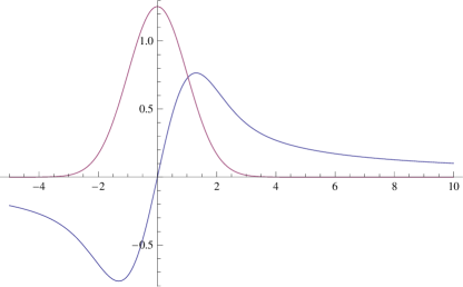
Figure 1.1. The imaginary part and the real part of $\Psi^{{\text{\rm{Catalan}}}}(x,1)$. For $x>>0$, the imaginary part dies down, and only the real part has a non-trivial asymptotic expansion. Thus (1.27) is a series with real coefficients.

One of the two independent solutions to the third example, the Gauß hypergeometric equation, that is holomorphic around $x=0$ is given by

(1.28) $$\Psi^{\text{\rm{Gau\ss}}}(x,\hbar)={}_{2}F_{1}\left(-\frac{\sqrt{(h-1)(h-3)}}{2h}+\frac{1}{h}-\frac{1}{2},\frac{\sqrt{(h-1)(h-3)}}{2h}+\frac{1}{h}-\frac{1}{2};\frac{1}{h};x\right),$$

where

(1.29) $${}_{2}F_{1}(a,b;c;x):=\sum_{n=0}^{\infty}\frac{(a)_{n}(b)_{n}}{(c)_{n}}\;\frac{x^{n}}{n!}$$

is the Gauß hypergeometric function. The topological recursion calculates the B-model genus expansion of the periods of the Legendre family of elliptic curves (1.19) at the point where the elliptic curve degenerates to a nodal rational curve. For example, the procedure applied to the spectral curve

$$y^{2}+\frac{2x-1}{x(x-1)}y+\frac{1}{4x(x-1)}=0$$

with a choice of

$$\eta=\frac{-(2x-1)-\sqrt{3x^{2}-3x+1}}{2x(x-1)}dx,$$

which is an eigenvalue $\alpha_{1}(x)$ of the Higgs field $\phi$, gives a genus expansion at $x=0$:

(1.30) $$\Psi^{\text{\rm{Gau\ss}}}(x,\hbar)=\exp\left(\sum_{g=0}^{\infty}\sum_{n=1}^{\infty}\frac{1}{n!}\hbar^{2g-2+n}F_{g,n}^{\text{\rm{Gau\ss}}}(x)\right).$$

At $\hbar=1$, we have a topological recursion expansion of the period $\omega_{1}(x)$ defined in (1.11):

(1.31) $$\frac{\omega_{1}(x)}{\pi}=\Psi^{\text{\rm{Gau\ss}}}(x,1)=\exp\left(\sum_{g=0}^{\infty}\sum_{n=1}^{\infty}\frac{1}{n!}F_{g,n}^{\text{\rm{Gau\ss}}}(x)\right).$$

A subtle point we notice here is that while the Gauß hypergeometric equation has regular singular points at $x=0,1,\infty$, the Hermite equation has an irregular singular point of class $2$ at $\infty$. The spectral curve of each case has an ordinary double point at $x=\infty$. But the crucial difference lies in the intersection of the spectral curve $\Sigma$ with the divisor $C_{\infty}$. For the Hermite case we have $\Sigma\cdot C_{\infty}=4$ and the intersection occurs all at once at $x=\infty$. For the Gauß hypergeometric case, the intersection $\Sigma\cdot C_{\infty}=4$ occurs once each at $x=0,1$, and twice at $x=\infty$. This confluence of regular singular points is the source of the irregular singularity in the Hermite differential equation.

The fourth row indicates an example of a quantum curve that has one regular singular point at $x=-1$ and one irregular singular point of class $1$ at $x=\infty$. The spectral curve has an ordinary double point at $x=\infty$, the same as the Hermite case. As Figure 1.2 shows, the class of the irregular singularity at $x=\infty$ is determined by how the spectral curve intersects with $C_{\infty}$.

  

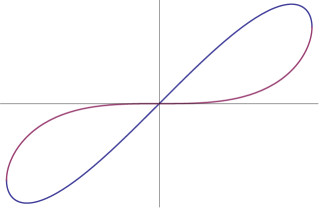
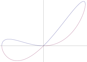
Figure 1.2. The spectral curves of the second and the fourth examples. The horizontal line is the divisor $C_{\infty}$, and the vertical line is the fiber class $F$ at $x=\infty$. The spectral curve intersects with $C_{\infty}$ a total of four times. The curve on the right has a triple intersection at $x=\infty$, while the one on the left intersects all at once.

The existence of the irregular singularity in the quantum curve associated with a spectral curve has nothing to do with the singularity of the spectral curve. The fifth example shows a non-singular spectral curve of genus $1$ (Figure 1.3), for which the quantum curve has a class $1$ irregular singularity at $x=\infty$.

Figure 1.3. The spectral curve of the fifth example, which is non-singular. The corresponding quantum curve has two regular singular points at $x=\pm 1$, and a class $1$ irregular singular point at $x=\infty$.

The paper is organized as follows. The general structure of the theory is explained using the Airy function as an example in Section 2. The notion of quantum curves as Rees $D$-modules quantizing Hitchin spectral curves is presented in Section 3. Since our topological recursion depends solely on the geometry of (1.6), the information of $\Sigma$ and $\widetilde{\Sigma}$, such as their arithmetic genera, becomes important. We will give the genus formulas in Sections 4 and 5. In Section 4 we study the geometry of the Hitchin spectral curves associated with rank $2$ meromorphic Higgs bundles. We give the genus formula for the normalization $\widetilde{\Sigma}$ in terms of the characteristic polynomial of the Higgs field $\phi$. A more systematic treatment of the spectral curve and its desingularization is given in Section 5. In Section 6, which is the heart of our paper, we prove the main theorem. Two more examples, Hermite differential equations and Gauß hypergeometric differential equations, are studied in Section 7.

2. A walk-through of the simplest example

Before going into the full generality, let us present the simplest example of our construction. With this example we can illustrate the relation between a Higgs bundle, the compactified cotangent bundle of a curve, a quantum curve, a classical differential equation, non-Abelian Hodge correspondence, and the quantum invariants that the quantum curve captures.

As a spectral curve, we take the algebraic curve $\Sigma\subset{\mathbb{F}}_{2}={\mathbb{P}}\left(K_{{\mathbb{P}}^{1}}\oplus{\mathcal{O}}_{{\mathbb{P}}^{1}}\right)=\overline{T^{*}{\mathbb{P}}^{1}}$ embedded in the Hirzebruch surface with the defining equation

(2.1) $$y^{2}-x=0.$$

Here, $x$ is the coordinate of the affine line ${\mathbb{A}}^{1}={\mathbb{P}}^{1}\setminus\{\infty\}$, and $y$ is the fiber coordinate of the cotangent bundle $T^{*}{\mathbb{P}}^{1}\subset{\mathbb{F}}^{2}$ over ${\mathbb{A}}^{1}$. The Hirzebruch surface is the natural compactification of the cotangent bundle $T^{*}{\mathbb{P}}^{1}$, which is the total space of the canonical bundle $K_{{\mathbb{P}}^{1}}$. We denote by $\eta\in H^{0}(T^{*}{\mathbb{P}}^{1},\pi^{*}K_{{\mathbb{P}}^{1}})$ the tautological $1$-form associated with the projection $\pi:T^{*}{\mathbb{P}}^{1}\longrightarrow{\mathbb{P}}^{1}$. It is expressed as $\eta=ydx$ in terms of the affine coordinates. The holomorphic symplectic form on $T^{*}{\mathbb{P}}^{1}$ is given by $-d\eta=dx\wedge dy$. The $1$-form $\eta$ extends to ${\mathbb{F}}_{2}$ as a meromorphic differential form and defines a divisor

(2.2) $$(\eta)=C_{0}-C_{\infty},$$

where $C_{0}$ is the zero-section of $T^{*}{\mathbb{P}}^{1}$, and $C_{\infty}$ the section at infinity of $\overline{T^{*}{\mathbb{P}}^{1}}$. The Picard group ${\text{\rm{Pic}}}({\mathbb{F}}_{2})$ of the Hirzebruch surface is generated by the class $C_{0}$ and a fiber class $F$ of $\pi$.

Although (2.1) is a perfect parabola in the affine plane, it has a quintic cusp singularity at $x=\infty$. Let $(u,w)$ be a coordinate on another affine piece of ${\mathbb{F}}_{2}$ defined by (1.20). Then $\Sigma$ in the $(u,w)$-plane is given by

(2.3) $$w^{2}=u^{5}.$$

The expression of $\Sigma$ as an element of ${\text{\rm{Pic}}}({\mathbb{F}}_{2})$ is thus given by $\Sigma=2C_{0}+5F.$ Define a stable Higgs pair $(E,\phi)$ with $E={\mathcal{O}}_{{\mathbb{P}}^{1}}\oplus{\mathcal{O}}_{{\mathbb{P}}^{1}}$ and

(2.4) $$\phi=\begin{bmatrix}&1\\ x\end{bmatrix}dx:E\longrightarrow E\otimes K_{{\mathbb{P}}^{1}}(2)=E.$$

Here, we choose a meromorphic $1$-form $xdx\in H^{0}\big{(}{\mathbb{P}}^{1},K_{{\mathbb{P}}^{1}}(2)\big{)}$ that has a simple zero at $0\in{\mathbb{P}}^{1}$ and a pole of order $3$ at $\infty\in{\mathbb{P}}^{1}$. Up to a constant factor, there is only one such differential $xdx=-du/u^{3}$. The spectral curve $\Sigma$ of $(E,\phi)$ is given by the characteristic equation

(2.5) $$\det(\eta-\pi^{*}\phi)=\eta^{2}-\pi^{*}{\text{\rm{tr}}}(\phi)+\pi^{*}\det(\phi)=0$$

in ${\mathbb{F}}_{2}$. The non-Abelian Hodge correspondence applied to $\phi$ determines a singular $\hbar$-connection [3, 41]

(2.6) $$\nabla^{\hbar}=\hbar d-\begin{bmatrix}&1\\ x\end{bmatrix}dx$$

on the trivial bundle $E={\mathcal{O}}_{{\mathbb{P}}^{1}}^{\oplus 2}$ over ${\mathbb{P}}^{1}$.

The quantization procedure that we will explain in this paper associates the following differential equation to the spectral curve $\Sigma$:

(2.7) $$\left(\left(\hbar\frac{d}{dx}\right)^{2}-x\right)\Psi(x,\hbar)=0.$$

The solution $\Psi$ gives rise to a flat section $\begin{bmatrix}\Psi\\ \Psi^{\prime}\end{bmatrix}$ of (2.6), where ^′ denotes the $x$ differentiation. The differential operator

(2.8) $$P(x,\hbar):=\left(\hbar\frac{d}{dx}\right)^{2}-x$$

quantizing (2.1) is an example of what we call a quantum curve. Reflecting the fact (2.3) that $\Sigma$ has a quintic cusp singularity at $x=\infty$, (2.7) has an irregular singular point of class $\frac{3}{2}$ at $x=\infty$. This number $\frac{3}{2}$ indicates how the asymptotic expansion of the solution looks like. Indeed, any non-trivial solution has an essential singularity at $\infty$. We note that every solution of (2.7) is an entire function for any value of $\hbar\neq 0$. Define

(2.9) $$a_{3n}=a_{0}\cdot\frac{\prod_{j=1}^{n}(3j-2)}{(3n)!},\qquad a_{3n+1}=a_{1}\cdot\frac{\prod_{j=1}^{n}(3j-1)}{(3n+1)!},\qquad a_{3n+2}=0,$$

for $n\geq 0$. Then

(2.10) $$\Psi(x,\hbar):=\sum_{n=0}^{\infty}a_{n}\left(\frac{x}{\hbar^{{2}/{3}}}\right)^{n}$$

gives an arbitrary solution to (2.7), which is entire. The coefficients (2.9) are of no particular interest.

What our quantization procedure tells us is a different, and more interesting, story. Applying our main result of this paper, we construct a particular all-order asymptotic expansion of this entire solution

(2.11) $$\Psi(x,\hbar)=\exp F(x,\hbar),\qquad F(x,\hbar):=\sum_{m=0}^{\infty}\hbar^{m-1}S_{m}(x),$$

valid for $|{\text{\rm{Arg}}}(x)|<\pi$, and $\hbar>0$. Here, the first two terms of the asymptotic expansion are given by

(2.12) $$S_{0}(x) =\pm\frac{2}{3}x^{\frac{3}{2}},$$

(2.13) $$S_{1}(x) =-\frac{1}{4}\log x.$$

Although the classical limit $\hbar\rightarrow 0$ of (2.7) does not make sense under the expansion (2.11), the semi-classical limit through the WKB analysis

(2.14) $$\left[e^{-S_{1}(x)}e^{-\frac{1}{\hbar}S_{0}(x)}\left(\hbar^{2}\frac{d^{2}}{dx^{2}}-x\right)e^{\frac{1}{\hbar}S_{0}(x)}e^{S_{1}(x)}\right]\exp\left(\sum_{m=2}^{\infty}\hbar^{m-1}S_{m}(x)\right)=0$$

has a well-defined limit $\hbar\rightarrow 0$. The result is $S_{0}^{\prime}(x)^{2}=x,$ which gives (2.12), and also (2.1) by defining $dS_{0}=\eta$. This process is called the semi-classical limit. The vanishing of the $\hbar$-linear terms of (2.14) is $2S_{0}^{\prime}(x)S_{1}^{\prime}(x)+S_{0}^{\prime\prime}(x)=0$, which gives (2.13) above.

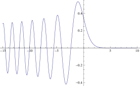
Figure 2.1. The Airy function

The solution we are talking about is the Airy function (1.21) for the choice of $S_{0}(x)=-\frac{2}{3}x^{\frac{3}{2}}$. This solution corresponds to (2.10) with the initial condition

$$a_{0}=\frac{1}{3^{\frac{2}{3}}\Gamma(\frac{2}{3})},\qquad a_{1}=-\frac{1}{3^{\frac{1}{3}}\Gamma(\frac{1}{3})}.$$

The surprising discovery of Kontsevich [38] is that $S_{m}(x)$ for $m\geq 2$ has the following closed formula:

(2.15) $$S_{m}(x):=\sum_{2g-2+n=m-1}\frac{1}{n!}F_{g,n}^{\text{Airy}}(x),$$

(2.16) $$F_{g,n}^{\text{Airy}}(x):=\frac{(-1)^{n}}{2^{2g-2+n}}\cdot x^{-\frac{(6g-6+3n)}{2}}\sum_{\begin{subarray}{c}d_{1}+\dots+d_{n}\\ =3g-3+n\end{subarray}}{\langle}\tau_{d_{1}}\cdots\tau_{d_{n}}{\rangle}_{g,n}\prod_{i=1}^{n}(2d_{i}-1)!!.$$

Although (2.15) is not a generating function of all intersection numbers, as we will show in the subsequent sections, the quantum curve (2.1) alone actually determines every intersection number ${\langle}\tau_{d_{1}}\cdots\tau_{d_{n}}{\rangle}_{g,n}$. This mechanism is the differential recursion equation of [18], based on the theory of integral topological recursion of [24], which computes free energies

(2.17) $$F_{g,n}^{\text{Airy}}(x_{1},\cdots,x_{n}):=\frac{(-1)^{n}}{2^{2g-2+n}}\sum_{\begin{subarray}{c}d_{1}+\dots+d_{n}\\ =3g-3+n\end{subarray}}{\langle}\tau_{d_{1}}\cdots\tau_{d_{n}}{\rangle}_{g,n}\prod_{i=1}^{n}\frac{(2d_{i}-1)!!}{\sqrt{x_{i}}^{2d_{i}+1}}$$

as a function in $n$ variables from $\Sigma$ through the process of blow-ups of ${\mathbb{F}}_{2}$.

Let us now give a detailed procedure for this example. We start with the spectral curve $\Sigma$ of (2.1). Our goal is to come up with (2.7). The first step is to blow up ${\mathbb{F}}_{2}$ and to construct (1.6). The discriminant of the defining equation (2.5) of the spectral curve is

$$-\det(\phi)=x(dx)^{2}=\frac{1}{u^{5}}(du)^{2}.$$

It has a simple zero at $x=0$ and a pole of order $5$ at $x=\infty$. The Geometric Genus Formula (4.12) tells us that $\widetilde{\Sigma}$ is a non-singular curve of genus $0$, i.e., a ${\mathbb{P}}^{1}$, after blowing up $\lfloor\frac{5}{2}\rfloor=2$ times. The center of blow-up is $(u,w)=(0,0)$ for the first time. Put $w=w_{1}u$, and denote by $E_{1}$ the exceptional divisor of the first blow-up. The proper transform of $\Sigma$ for this blow-up, $w_{1}^{2}=u^{3}$, has a cubic cusp singularity, so we blow up again at the singular point. Let $w_{1}=w_{2}u$, and denote by $E_{2}$ the exceptional divisor created by the second blow-up. The self-intersection of the proper transform of $E_{1}$ is $-2$. We then obtain the desingularized curve $\Sigma_{\min}$, locally given by $w_{2}^{2}=u$. The proof of Theorem 4.2 also tells us that $\Sigma_{\min}\longrightarrow{\mathbb{P}}^{1}$ is ramified at two points. Choose the affine coordinate $t=2w_{2}$ of the exceptional divisor added at the second blow-up. Our choice of the constant factor is to make the formula the same as in [19]. We have

(2.18) $$\begin{cases}x=\frac{1}{u}=\frac{1}{w_{2}^{2}}=\frac{4}{t^{2}}\\ y=-\frac{u^{2}}{w}=-\frac{u^{2}}{w_{2}u^{2}}=-\frac{2}{t}.\end{cases}$$

In the $(u,w)$-coordinate, we see that the parameter $t$ is a normalization parameter of the quintic cusp singularity:

$$\begin{cases}u=\frac{t^{2}}{4}\\ w=\frac{t^{5}}{32}.\end{cases}$$

Note that $\Sigma_{\min}$ intersects transversally with the proper transform of $C_{\infty}$. We blow up once again at this intersection, and denote by $\widetilde{\Sigma}$ the proper transform of $\Sigma_{\min}$. The blow-up space $Bl({\mathbb{F}}^{2})$ is the result of $3=\lceil\frac{5}{2}\rceil$ times blow-ups of the Hirzebruch surface.

Now we apply the differential recursion (6.11) to the geometric data (1.6) and (1.7). We claim that the integral topological recursion of [24] for the geometric data we are considering now is exactly the same as the integral topological recursion of [19, (6.12)] applied to the curve (2.18) realized as a plane parabola in ${\mathbb{C}}^{2}$. This is because our integral topological recursion (6.10) has two residue contributions, one each from $t=0$ and $t=\infty$. As proved in [19, Section 6], the integrand on the right-hand side of the integral recursion formula [19, (6.12)] does not have any pole at $t=0$. Therefore, the residue contribution from this point is $0$. The differential recursion is obtained by deforming the contour of integration to enclose only poles of the differential forms $W_{g,n}$. Since $t=0$ is a regular point, the two methods have no difference.

The $W_{0,2}$ of (1.7) is simply $\frac{dt_{1}\cdot dt_{2}}{(t_{1}-t_{2})^{2}}$ because $\widetilde{\Sigma}\cong{\mathbb{P}}^{1}$. Since $t$ of (2.18) is a normalization coordinate, we have

$$W_{0,1}=\tilde{i}^{*}\nu^{*}(\eta)=y(t)dx(t)=\frac{16}{t^{4}},$$

in agreement of [19, (6.8)]. Noting that the solution to the integral topological recursion is unique from the initial data, we conclude that

$$d_{1}\cdots d_{n}F_{g,n}^{\text{\rm{Airy}}}\big{(}x(t_{1}),\dots,x(t_{n})\big{)}=W_{g,n}.$$

By setting the constants of integration by integrating from $t=0$ for the differential recursion equation, we obtain the expression (2.17). Then its principal specialization gives (2.16). The equivalence of the differential recursion and the quantum curve equation Theorem 6.1 then proves (2.7) with the expression of (2.11) and (2.15).

In this process, what is truly amazing is that the single differential equation (2.7), which is our quantum curve in this case, knows everything about the free energies (2.17). This is because we can recover the spectral curve $\Sigma$ from the quantum curve. Then the procedures we need to apply, the blow-ups and the differential recursion equation, are canonical. Therefore, we do recover (2.17) as explained above.

It is surprising to see that a simple entire function (2.10) contains so much geometric information. Our expansion (2.11) is an expression of an entire function viewed from its essential singularity. We can extract rich information of the solution by restricting the region where the asymptotic expansion is valid. If we consider (2.11) only as a formal expression in $x$ and $\hbar$, then we cannot see how the coefficients are related to quantum invariants. The topological recursion [24] is a key to connect the two worlds: the world of quantum invariants, and the world of holomorphic functions and differentials. This relation is also knows as a mirror symmetry, or in analysis, simply as the Laplace transform. The intersection numbers ${\langle}\tau_{d_{1}}\cdots\tau_{d_{n}}{\rangle}_{g,n}$ belong to the $A$-model, while the spectral curve $\Sigma$ of (2.1) and free energies belong to the $B$-model. We consider (2.17) as an example of the Laplace transform, playing the role of mirror symmetry [19].

3. Quantum curves for Higgs bundles

In this section, we give the definition of quantum curves. Let $C$ be a non-singular projective algebraic curve defined over ${\mathbb{C}}$. The sheaf ${\mathcal{D}}_{C}$ of differential operators on $C$ is the subalgebra generated by the anti-canonical sheaf $K_{C}^{-1}$ and the structure sheaf ${\mathcal{O}}_{C}$ in the ${\mathbb{C}}$-linear endomorphism algebra ${\mathcal{E}}nd_{{\mathbb{C}}}({\mathcal{O}}_{C})$. Here, $K_{C}^{-1}$ acts on ${\mathcal{O}}_{C}$ as holomorphic vector fields, and ${\mathcal{O}}_{C}$ acts on itself by multiplication. Locally every element of ${\mathcal{D}}_{C}$ is written as

$${\mathcal{D}}_{C}\owns P(x)=\sum_{\ell=0}^{r}a_{\ell}(x)\left(\frac{d}{dx}\right)^{r-\ell},\qquad a_{\ell}(x)\in{\mathcal{O}}_{C}$$

for some $r\geq 0$. For a fixed $r$, we introduce the filtration by order of differential operators into ${\mathcal{D}}_{C}$ as follows:

$$F_{r}{\mathcal{D}}_{C}=\left.\left\{P(x)=\sum_{\ell=0}^{r}a_{\ell}(x)\left(\frac{d}{dx}\right)^{r-\ell}\right|a_{\ell}(x)\in{\mathcal{O}}_{C}\right\}.$$

The Rees ring $\widetilde{{\mathcal{D}}_{C}}$ is defined by

(3.1) $$\widetilde{{\mathcal{D}}_{C}}=\bigoplus_{r=0}^{\infty}\hbar^{r}F_{r}{\mathcal{D}}_{C}\subset{\mathbb{C}}[\hbar]\otimes_{\mathbb{C}}{\mathcal{D}}_{C}.$$

An element of $\widetilde{{\mathcal{D}}_{C}}$ on a coordinate neighborhood $U\subset C$ can be written uniquely as

(3.2) $$P(x,\hbar)=\sum_{\ell=0}^{r}a_{\ell}(x)\left(\hbar\frac{d}{dx}\right)^{r-\ell}$$

(see [41, Section 1.5]).

Definition 3.1 (Quantum curve).

A quantum curve is the Rees $\widetilde{{\mathcal{D}}_{C}}$-module

(3.3) $$\widetilde{{\mathcal{M}}}=\bigoplus_{r=0}^{\infty}\hbar^{r}F_{r}{\mathcal{M}}$$

associated with a filtered ${\mathcal{D}}_{C}$-module $({\mathcal{M}},F_{r})$ defined on $C$, with the compatibility

$$F_{a}{\mathcal{D}}_{C}\cdot F_{b}{\mathcal{M}}\subset F_{a+b}{\mathcal{M}}.$$

Let

$$D=\sum_{j=1}^{n}m_{j}p_{j},\qquad m_{j}>0$$

be an effective divisor on $C$. The point set $\{p_{1},\dots,p_{n}\}\subset C$ is the support of $D$. A meromorphic Higgs bundle with poles at $D$ is a pair $(E,\phi)$ consisting of an algebraic vector bundle $E$ on $C$ and a Higgs field

(3.4) $$\phi:E\longrightarrow K_{C}(D)\otimes_{{\mathcal{O}}_{C}}E.$$

Since the cotangent bundle

$$T^{*}C={\text{\rm{Spec}}}\left({\text{\rm{Sym}}}\left(K_{C}^{-1}\right)\right)$$

is the total space of $K_{C}$, we have the tautological $1$-form $\eta\in H^{0}(T^{*}C,\pi^{*}K_{C})$ on $T^{*}C$ coming from the projection

$$\begin{CD}T^{*}C@<{}<{}<\pi^{*}K_{C}\\ @V{\pi}V{}V\\ C@<{}<{}<K_{C}.\end{CD}$$

The natural holomorphic symplectic form of $T^{*}C$ is given by $-d\eta$. The compactified cotangent bundle of $C$ is a ruled surface defined by

(3.5) $$\overline{T^{*}C}:={\mathbb{P}}\left(K_{C}\oplus{\mathcal{O}}_{C}\right)={\text{\rm{Proj}}}\left(\bigoplus_{n=0}^{\infty}\left(K_{C}^{-n}\cdot I^{0}\oplus K_{C}^{-n+1}\cdot I\oplus\cdots\oplus K_{C}^{0}\cdot I^{n}\right)\right),$$

where $I$ represents $1\in{\mathcal{O}}_{C}$ being considered as a degree $1$ element. The divisor at infinity $C_{\infty}$ of (1.5) is reduced in the ruled surface and supported on the subset ${\mathbb{P}}\left(K_{C}\oplus{\mathcal{O}}_{C}\right)\setminus T^{*}C$. The tautological form $\eta$ extends on $\overline{T^{*}C}$ as a meromorphic $1$-form with simple poles along $C_{\infty}$. Thus the divisor of $\eta$ in $\overline{T^{*}C}$ is given by

(3.6) $$(\eta)=C_{0}-C_{\infty},$$

where $C_{0}$ is the zero section of $T^{*}C$.

The relation between the sheaf ${\mathcal{D}}_{C}$ and the geometry of the compactified cotangent bundle $\overline{T^{*}C}$ is the following. First we have

(3.7) $${\text{\rm{Spec}}}\left(\bigoplus_{m=0}^{\infty}F_{m}{\mathcal{D}}_{C}\big{/}F_{m-1}{\mathcal{D}}_{C}\right)={\text{\rm{Spec}}}\left(\bigoplus_{m=0}^{\infty}K_{C}^{-m}\right)=T^{*}C.$$

Let us denote by $gr_{m}{\mathcal{D}}_{C}=F_{m}{\mathcal{D}}_{C}\big{/}F_{m-1}{\mathcal{D}}_{C}$. By writing $I=1\in H^{0}(C,{\mathcal{D}}_{C})$, we then have

(3.8) $${\text{\rm{Proj}}}\left(\bigoplus_{m=0}^{\infty}\left(gr_{m}{\mathcal{D}}_{C}\cdot I^{0}\oplus gr_{m-1}{\mathcal{D}}_{C}\cdot I\oplus gr_{m-2}{\mathcal{D}}_{C}\cdot I^{\otimes 2}\oplus\cdots\oplus gr_{0}{\mathcal{D}}_{C}\cdot I^{\otimes m}\right)\right)\\ =\overline{T^{*}C}.$$

Definition 3.2 (Spectral curve).

A spectral curve of degree $r$ is a divisor $\Sigma$ in $\overline{T^{*}C}$ such that the projection $\pi:\Sigma\longrightarrow C$ defined by the restriction

is a finite morphism of degree $r$. The spectral curve of a Higgs bundle $(E,\phi)$ is the divisor of zeros

(3.9) $$\Sigma=\left(\det(\eta-\pi^{*}\phi)\right)_{0}$$

on $\overline{T^{*}C}$ of the characteristic polynomial $\det(\eta-\pi^{*}\phi)$. Here,

$$\pi^{*}\phi:\pi^{*}E\longrightarrow\pi^{*}\left(K_{C}(D)\right)\otimes_{{\mathcal{O}}_{{\mathbb{P}}\left(K_{C}\oplus{\mathcal{O}}_{C}\right)}}\pi^{*}E.$$

Remark 3.3.

The Higgs field $\phi$ is holomorphic on $C\setminus{\text{\rm{supp}}}(D)$. Thus we can define the divisor of zeros

$$\Sigma^{\circ}=\left(\det\left(\eta-\pi^{*}\left(\phi|_{C\setminus{\text{\rm{supp}}}(D)}\right)\right)\right)_{0}$$

of the characteristic polynomial on $T^{*}(C\setminus{\text{\rm{supp}}}(D))$. The spectral curve $\Sigma$ is the complex topology closure of $\Sigma^{\circ}$ with respect to the compactification

(3.10) $$T^{*}(C\setminus{\text{\rm{supp}}}(D))\subset\overline{T^{*}C}.$$

A left ${\mathcal{D}}_{C}$-module ${\mathcal{E}}$ on $C$ is naturally an ${\mathcal{O}}_{C}$-module with a ${\mathbb{C}}$-linear integrable connection $\nabla:{\mathcal{E}}\longrightarrow K_{C}\otimes_{{\mathcal{O}}_{C}}{\mathcal{E}}$. The construction goes as follows:

(3.11) $$\begin{CD}\nabla:{\mathcal{E}}@>{\alpha}>{}>{\mathcal{D}}_{C}\otimes_{{\mathcal{O}}_{C}}{\mathcal{E}}@>{\nabla_{\!{\mathcal{D}}}\otimes id}>{}>\left(K_{C}\otimes_{{\mathcal{O}}_{C}}{\mathcal{D}}_{C}\right)\otimes_{{\mathcal{O}}_{C}}{\mathcal{E}}@>{\beta\otimes id}>{}>K_{C}\otimes_{{\mathcal{O}}_{C}}{\mathcal{E}},\end{CD}$$

where

• $\alpha$ is the natural inclusion ${\mathcal{E}}\owns v\longmapsto 1\otimes v\in{\mathcal{D}}_{C}\otimes_{{\mathcal{O}}_{C}}{\mathcal{E}}$;

• $\nabla_{\!{\mathcal{D}}}:{\mathcal{D}}_{C}\longrightarrow K_{C}\otimes_{{\mathcal{O}}_{C}}{\mathcal{D}}_{C}$ is the connection defined by the ${\mathbb{C}}$-linear left-multiplication operation of $K_{C}^{-1}$ on ${\mathcal{D}}_{C}$, which satisfies the derivation property

  (3.12) $$\nabla_{\!{\mathcal{D}}}(f\cdot P)=f\cdot\nabla_{\!{\mathcal{D}}}(P)+df\cdot P\in K_{C}\otimes_{{\mathcal{O}}_{C}}{\mathcal{D}}_{C}$$

  for $f\in{\mathcal{O}}_{C}$ and $P\in{\mathcal{D}}_{C}$; and

• $\beta$ is the canonical right ${\mathcal{D}}_{C}$-module structure in $K_{C}$.

If we choose a local coordinate neighborhood $U\subset C$ with a coordinate $x$, then (3.12) takes the following form. Let us denote by $P^{\prime}=[d/dx,P]-P\cdot d/dx$, and define

$$\nabla_{\!\!\frac{d}{dx}}(P):=P\cdot\frac{d}{dx}+P^{\prime}.$$

Then we have

$$\nabla_{\!\!\frac{d}{dx}}(f\cdot P)=f\cdot\nabla_{\!\!\frac{d}{dx}}(P)+\frac{df}{dx}\cdot P.$$

The connection $\nabla$ of (3.11) is integrable because $d^{2}=1$. Actually, the statement is true for any dimensions. We note that there is no reason for ${\mathcal{E}}$ to be coherent as an ${\mathcal{O}}_{C}$-module.

Conversely, if an algebraic vector bundle $E$ on $C$ of rank $r$ admits a holomorphic connection $\nabla:E\longrightarrow K_{C}\otimes E$, then $E$ acquires the structure of a ${\mathcal{D}}_{C}$-module. This is because $\nabla$ is automatically flat, and the covariant derivative $\nabla_{\!X}$ for $X\in K_{C}^{-1}$ satisfies

(3.13) $$\nabla_{\!X}(fv)=f\nabla_{\!X}(v)+X(f)v$$

for $f\in{\mathcal{O}}_{C}$ and $v\in E$. A repeated application of (3.13) makes $E$ a ${\mathcal{D}}_{C}$-module. The fact that every ${\mathcal{D}}_{C}$-module on a curve is principal implies that for every point $p\in C$, there is an open neighborhood $p\in U\subset C$ and a linear differential operator $P$ of oder $r$ on $U$, called a generator, such that $E|_{U}\cong{\mathcal{D}}_{U}/{\mathcal{D}}_{U}P.$ Thus on an open curve $U$, a holomorphic connection in a vector bundle of rank $r$ gives rise to a differential operator of order $r$. The converse is true if ${\mathcal{D}}_{U}/{\mathcal{D}}_{U}P$ is ${\mathcal{O}}_{U}$-coherent.

Definition 3.4 ($\hbar$-connection).

A holomorphic $\hbar$-connection on a vector bundle $E\longrightarrow C$ is a ${\mathbb{C}}[\hbar]$-linear homomorphism

$$\nabla^{\hbar}:{\mathbb{C}}[\hbar]\otimes E\longrightarrow{\mathbb{C}}[\hbar,\hbar^{-1}]\otimes K_{C}\otimes_{{\mathcal{O}}_{C}}E$$

subject to the derivation condition

(3.14) $$\nabla^{\hbar}(f\cdot v)=f\nabla^{\hbar}(v)+\hbar df\otimes v,$$

where $f\in{\mathcal{O}}_{C}\otimes{\mathbb{C}}[\hbar]$ and $v\in{\mathbb{C}}[\hbar]\otimes E$.

Remark 3.5.

The classical limit of a holomorphic $\hbar$-connection is the evaluation $\hbar=0$ of $\nabla^{\hbar}$, which is simply an ${\mathcal{O}}_{C}$-module homomorphism

$$\nabla^{0}:E\longrightarrow K_{C}\otimes_{{\mathcal{O}}_{C}}E,$$

i.e., a holomorphic Higgs field in the vector bundle $E$.

Remark 3.6.

An ${\mathcal{O}}_{C}\otimes{\mathbb{C}}[\hbar]$-coherent $\widetilde{{\mathcal{D}}_{C}}$-module is equivalent to a vector bundle on $C$ equipped with an $\hbar$-connection.

In analysis, the semi-classical limit of a differential operator $P(x,\hbar)$ of (3.2) is defined by

(3.15) $$\lim_{\hbar\rightarrow 0}\left(e^{-\frac{1}{\hbar}S_{0}(x)}P(x,\hbar)e^{\frac{1}{\hbar}S_{0}(x)}\right)=\sum_{\ell=0}^{r}a_{\ell}(x)\left(S_{0}^{\prime}(x)\right)^{r-\ell},$$

where $S_{0}(x)\in{\mathcal{O}}_{C}(U)$. The equation

(3.16) $$\lim_{\hbar\rightarrow 0}\left(e^{-\frac{1}{\hbar}S_{0}(x)}P(x,\hbar)e^{\frac{1}{\hbar}S_{0}(x)}\right)=0$$

then determines the first term of the singular perturbation expansion

(3.17) $$\Psi(x,\hbar)=\exp\left(\sum_{m=0}^{\infty}\hbar^{m-1}S_{m}(x)\right)$$

of the solution $\Psi(x,\hbar)$ of the differential equation

$$P(x,\hbar)\Psi(x,\hbar)=0$$

on U. Since $dS_{0}(x)$ is a local section of $T^{*}C$ on $U\subset C$, $y=S_{0}^{\prime}(x)$ gives the local trivialization of $T^{*}C|_{U}$, with $y\in T_{x}^{*}C$ a fiber coordinate. Equations (3.15) and (3.16) then give an equation

(3.18) $$\sum_{\ell=0}^{r}a_{\ell}(x)y^{r-\ell}=0$$

of a curve in $T^{*}C|_{U}$. This motivates us to give the following definition:

Definition 3.7 (Semi-classical limit of a Rees differential operator).

Let $U\subset C$ be an open subset of $C$ with a local coordinate $x$ such that $T^{*}C$ is trivial over $U$ with a fiber coordinate $y$. The semi-classical limit of a local section

$$P(x,\hbar)=\sum_{\ell=0}^{r}a_{\ell}(x)\left(\hbar\frac{d}{dx}\right)^{r-\ell}$$

of the Rees ring $\widetilde{{\mathcal{D}}_{C}}$ of the sheaf of differential operators ${\mathcal{D}}_{C}$ on $U$ is the holomorphic function

$$\sum_{\ell=0}^{r}a_{\ell}(x)y^{r-\ell}$$

defined on $T^{*}C|_{U}$.

Definition 3.8 (Semi-classical limit).

Suppose a Rees $\widetilde{{\mathcal{D}}_{C}}$-module $\widetilde{{\mathcal{M}}}$ is written as

(3.19) $$\widetilde{{\mathcal{M}}}(U)=\widetilde{{\mathcal{D}}_{C}}(U)\big{/}\widetilde{{\mathcal{D}}_{C}}(U)P_{U}$$

on every coordinate neighborhood $U\subset C$ with a differential operator $P_{U}$ of the form (3.2). Using this expression (3.2) for $P_{U}$, we construct a meromorphic function

(3.20) $$p_{U}(x,y)=\sum_{\ell=0}^{r}a_{\ell}(x)y^{r-\ell}$$

on $\overline{T^{*}C}|_{U}$, where $y$ is the fiber coordinate of $T^{*}C$, which is trivialized on $U$. Define

(3.21) $$\Sigma_{U}=(p_{U}(x,y))_{0}$$

as the divisor of zero of the function $p_{U}(x,y)$. If $\Sigma_{U}$’s glue together to a spectral curve $\Sigma\subset\overline{T^{*}C}$, then we call $\Sigma$ the semi-classlical limit of the Rees $\widetilde{{\mathcal{D}}_{C}}$-module $\widetilde{{\mathcal{M}}}$.

Remark 3.9.

For the local equation (3.20) to be consistent globally on $C$, the coefficients of (3.2) have to satisfy

(3.22) $$a_{\ell}(x)\in\Gamma\!\left(U,K_{C}^{\otimes\ell}\right).$$

Definition 3.10 (Quantum curve for holomorphic Higgs bundle).

A quantum curve associated with the spectral curve $\Sigma\subset T^{*}C$ of a holomorphic Higgs bundle on a projective algebraic curve $C$ is a Rees $\widetilde{{\mathcal{D}}_{C}}$-module ${\mathcal{E}}$ whose semi-classical limit is $\Sigma$.

The main reason we need to extend our framework to meromorphic connections is that there are no non-trivial holomorphic connections on ${\mathbb{P}}^{1}$, whereas many important classical examples of differential equations are naturally defined over ${\mathbb{P}}^{1}$ with regular and irregular singularities. A ${\mathbb{C}}$-linear homomorphism

$$\nabla:E\longrightarrow K_{C}(D)\otimes_{{\mathcal{O}}_{C}}E$$

is said to be a meromorphic connection with poles along an effective divisor $D$ if

$$\nabla(f\cdot v)=f\nabla(v)+df\otimes v$$

for every $f\in{\mathcal{O}}_{C}$ and $v\in E$. Let us denote by

$${\mathcal{O}}_{C}(*D):=\lim_{\longrightarrow}{\mathcal{O}}_{C}(mD),\qquad E(*D):=E\otimes_{{\mathcal{O}}_{C}}{\mathcal{O}}_{C}(*D).$$

Then $\nabla$ extends to

$$\nabla:E(*D)\longrightarrow K_{C}(*D)\otimes_{{\mathcal{O}}_{C}(*D)}E(*D).$$

Since $\nabla$ is holomorphic on $C\setminus{\text{\rm{supp}}}(D)$, it induces a ${\mathcal{D}}_{C\setminus{\text{\rm{supp}}}(D)}$-module structure in $E|_{C\setminus{\text{\rm{supp}}}(D)}$. The ${\mathcal{D}}_{C}$-module direct image $\widetilde{E}=j_{*}\left(E|_{C\setminus{\text{\rm{supp}}}(D)}\right)$ associated with the open inclusion map $j:C\setminus{\text{\rm{supp}}}(D)\longrightarrow C$ is then naturally isomorphic to

(3.23) $$\widetilde{E}=j_{*}\left(E|_{C\setminus{\text{\rm{supp}}}(D)}\right)\cong E(*D)$$

as a ${\mathcal{D}}_{C}$-module. (3.23) is called the meromorphic extension of the ${\mathcal{D}}_{C\setminus{\text{\rm{supp}}}(D)}$-module $E|_{C\setminus{\text{\rm{supp}}}(D)}$.

Let us take a local coordinate $x$ of $C$, this time around a pole $p_{j}\in{\text{\rm{supp}}}(D)$. If a generator $\widetilde{P}$ of $\widetilde{E}$ near $x=0$ has a local expression

(3.24) $$\widetilde{P}(x,d/dx)=x^{k}\sum_{\ell=0}^{r}b_{\ell}(x)\left(x\frac{d}{dx}\right)^{r-\ell}$$

around $p_{j}$ with locally defined holomorphic functions $b_{\ell}(x)$, $b_{0}(0)\neq 0$, and an integer $k\in{\mathbb{Z}}$, then $\widetilde{P}$ has a regular singular point at $p_{j}$. Otherwise, $p_{j}$ is an irregular singular point of $\widetilde{P}$.

Definition 3.11 (Quantum curve for a meromorphic Higgs bundle).

Let $(E,\phi)$ be a meromorphic Higgs bundle defined over a projective algebraic curve $C$ of any genus with poles along an effective divisor $D$, and $\Sigma\subset\overline{T^{*}C}$ its spectral curve. A quantum curve associated with $\Sigma$ is the meromorphic extension of a Rees $\widetilde{{\mathcal{D}}_{C}}$-module ${\mathcal{E}}$ on $C\setminus{\text{\rm{supp}}}(D)$ such that the closure of its semi-classical limit $\Sigma^{\circ}\subset T^{*}C|_{C\setminus{\text{\rm{supp}}}(D)}$ in the compactified cotangent bundle $\overline{T^{*}C}$ agrees with $\Sigma$.

4. Geometry of spectral curves in the compactified cotangent bundle

To construct quantum curves using the topological recursion, we need a smooth Eynard-Orantin spectral curve [24] for which we can apply the recursion mechanism. When the given Hitchin spectral curve $\Sigma$ is singular, we have to find a non-singular model. In this paper we use the normalization $\widetilde{\Sigma}$ of the singular spectral curve. Since the quantum curve reflects the geometry of $\Sigma\subset\overline{T^{*}C}$, it is important to identify the choice of the blow-up space $Bl(\overline{T^{*}C})$ of (1.6) in which $\widetilde{\Sigma}$ is realized as a smooth divisor. We then determine the initial value $W_{0,1}$ for the topological recursion.

The geometry of a spectral curve also gives us the information of the singularity of the quantum curve. For example, when we have a component of a spectral curve tangent to the divisor $C_{\infty}$, the quantum curve has an irregular singular point, and the class of the irregularity is determined by the degree of tangency. We will give a classification of the singularity of the quantum curves in terms of the geometry of spectral curves in Section 6.3.

In this section, we give the construction of the canonical blow-up space $Bl(\overline{T^{*}C})$, and determine the genus of the normalization $\widetilde{\Sigma}$. This genus is necessary to identify the Riemann prime form on it, which determines another input datum $W_{0,2}$ for the topological recursion.

There are two different ways of defining the spectral curve for Higgs bundles with meromorphic Higgs field. Our definition of the previous section uses the compactified cotangent bundle. This idea also appears in [39]. The traditional definition, which assumes the pole divisor $D$ of the Higgs field to be reduced, is suitable for the study of moduli spaces of parabolic Higgs bundles. When we deal with non-reduced effective divisors, parabolic structures do not play any role. Non-reduced divisors appear naturally when we deal with classical equations such as the Airy differential equation, which has an irregular singular point of class $\frac{3}{2}$ at $\infty\in{\mathbb{P}}^{1}$.

Our point of view of spectral curves is also closely related to considering the stable pairs of pure dimension $1$ on $\overline{T^{*}C}$. Through Hitchin’s abelianization idea, the moduli space of stable pairs and the moduli space of Higgs bundles are identified [36].

Let $E$ be an algebraic vector bundle of rank $2$ on a non-singular projective algebraic curve $C$ of genus $g$, and

$$\phi:E\longrightarrow K_{C}(D)\otimes_{{\mathcal{O}}_{C}}E$$

a meromorphic Higgs field with poles along an effective divisor $D$. The trace and the determinant of $\phi$,

(4.1) $$a_{1}:=-{\text{\rm{tr}}}(\phi) \in H^{0}\left(C,K_{C}(D)\right),$$

(4.2) $$a_{2}:=\det(\phi) \in H^{0}\left(C,K_{C}^{\otimes 2}(2D)\right),$$

are well defined and determine the spectral curve $\Sigma$ of (3.9). For the purpose of investigating the geometry of $\Sigma$, we do not need the information of the Higgs bundle $(E,\phi)$, or even the pole divisor $D$. Thus in what follows, we only assume that $a_{1}$ is a meromorphic section of $K_{C}$, and that $a_{2}$ a meromorphic section of $K_{C}^{\otimes 2}$. Then the spectral curve is re-defined as the zero-locus in $\overline{T^{*}C}$ of a quadratic equation with $a_{1}$ and $a_{2}$ its coefficients:

(4.3) $$\Sigma:=\left(\eta^{2}+\pi^{*}(a_{1})\eta+\pi^{*}(a_{2})\right)_{0}.$$

The only condition we impose here is that the spectral curve is irreducible. In the language of Higgs bundles, this condition corresponds to the stability of $(E,\phi)$.

Recall that ${\text{\rm{Pic}}}(\overline{T^{*}C})$ is generated by the zero section $C_{0}$ of $T^{*}C$ and fibers of the projection map $\pi:\overline{T^{*}C}\longrightarrow C$. Since the spectral curve $\Sigma$ is a double covering of $C$, as a divisor it is expressed as

(4.4) $$\Sigma=2C_{0}+\sum_{j=1}^{a}\pi^{*}(p_{j})\in{\text{\rm{Pic}}}(\overline{T^{*}C}),$$

where $\alpha=\sum_{j=1}^{a}p_{j}\in{\text{\rm{Pic}}}^{a}(C)$ is a divisor on $C$ of degree $a$. As an element of the Néron-Severi group

$${\text{\rm{NS}}}(\overline{T^{*}C})={\text{\rm{Pic}}}(\overline{T^{*}C})/{\text{\rm{Pic}}}^{0}(\overline{T^{*}C}),$$

it is simply

$$\Sigma=2C_{0}+aF\in{\text{\rm{NS}}}(\overline{T^{*}C})$$

for a typical fiber class $F$. Since the intersection $FC_{\infty}=1$, we have $a=\Sigma C_{\infty}$ in ${\text{\rm{NS}}}(\overline{T^{*}C})$. From the genus formula

$$p_{a}(\Sigma)={\frac{1}{2}}\Sigma\cdot(\Sigma+K_{\overline{T^{*}C}})+1$$

and

$$K_{\overline{T^{*}C}}=-2C_{0}+(4g-4)F\in{\text{\rm{NS}}}(\overline{T^{*}C}),$$

we find that the arithmetic genus of the spectral curve $\Sigma$ is

(4.5) $$p_{a}(\Sigma)=4g-3+a,$$

where $a$ is the number of intersections of $\Sigma$ and $C_{\infty}$. Now we wish to find the geometric genus of $\Sigma$.

Motivated by the completion of square expression of the defining equation (4.3),

(4.6) $$\eta^{2}+\pi^{*}(a_{1})\eta+\pi^{*}(a_{2})=\left(\eta+{\frac{1}{2}}\pi^{*}(a_{1})\right)^{2}-\left(\frac{1}{4}\pi^{*}(a_{1})^{2}-\pi^{*}(a_{2})\right)$$

as a meromorphic section of $\pi^{*}K_{C}^{\otimes 2}$, we give the following definition.

Definition 4.1 (Discriminant divisor).

The discriminant divisor of the spectral curve (4.3) is a divisor on $C$ defined by

(4.7) $$\Delta:=\left(\frac{1}{4}a_{1}^{2}-a_{2}\right)=\Delta_{0}-\Delta_{\infty},$$

where

(4.8) $$\Delta_{0}=\sum_{i=1}^{m}m_{i}q_{i},\quad m_{i}>0,\quad q_{i}\in C,$$

(4.9) $$\Delta_{\infty}=\sum_{j=1}^{n}n_{j}p_{j},\quad n_{j}>0,\quad p_{j}\in C.$$

Since $\frac{1}{4}a_{1}^{2}-a_{2}$ is a meromorphic section of $K_{C}^{\otimes 2}$, we have

(4.10) $$\deg\Delta=\sum_{i=1}^{m}m_{i}-\sum_{j=1}^{n}n_{j}=4g-4.$$

Theorem 4.2 (Geometric genus formula).

Let us define an invariant of the discriminant divisor by

(4.11) $$\delta=|\{i\;|\;m_{i}\equiv 1\mod 2\}|+|\{j\;|\;n_{j}\equiv 1\mod 2\}|.$$

Then the geometric genus of the spectral curve $\Sigma$ of (4.3) is given by

(4.12) $$\tilde{g}:=p_{g}(\Sigma)=2g-1+{\frac{1}{2}}\delta.$$

We note that (4.10) implies $\delta\equiv 0\mod 2$.

Remark 4.3.

If $\phi$ is a holomorphic Higgs field, then $a_{1}=-{\text{\rm{tr}}}(\phi)$, $a_{2}=\det(\phi)$, and

$$m=\delta=4g-4,\quad n=0.$$

Therefore we have $\tilde{g}=4g-3$, which agrees with the genus formula of [18, Eq.(2.5)].

Before giving the proof of the formula, first we wish to identify the geometric meaning of the invariant $\delta$. Since $\Sigma\subset\overline{T^{*}C}$ is a double covering of $C$ in a ruled surface, locally at every singular point $p$, $\Sigma$ is either irreducible, or reducible and consisting of two components. When irreducible, it is locally isomorphic to

(4.13) $$t^{2}-s^{2m+1}=0,\qquad m\geq 1.$$

If it has two components, then it is locally isomorphic to

(4.14) $$t^{2}-s^{2m}=(t-s^{m})(t+s^{m})=0.$$

Since the local form of $\Sigma$ at a ramification point of $\pi:\Sigma\longrightarrow C$ is written as (4.13) with $m=0$, by extending the terminology “singularity” to “critical points” of the morphism $\pi$, we include a ramification point as a cusp with $m=0$.

Proposition 4.4.

The invariant $\delta$ of (4.11) counts the number of cusps of the spectral curve $\Sigma$.

Thus we have

(4.15) $$p_{g}(\Sigma)=2g(C)-1+{\frac{1}{2}}\;(\text{\rm{the number of cusps}}).$$

Proof of (4.15), assuming Proposition 4.4.

Let $\nu_{\min}:\Sigma_{\min}\longrightarrow\Sigma$ be the minimal resolution of singularities of $\Sigma$. Then $\pi_{\min}=\pi\circ\nu_{\min}:\Sigma_{\min}\longrightarrow C$ is a double sheeted covering of $C$ by a smooth curve $\Sigma_{\min}$. If $\Sigma$ has two components at a singularity $P$ as in (4.14), then $\pi_{\min}^{-1}(P)$ consists of two points and $\pi_{\min}$ is not ramified there. If $P$ is a cusp (4.13), then $\pi_{\min}^{-1}(P)$ is a ramification point of the covering $\pi_{\min}$. If $\delta$ counts the total number of cusp singularities and the ramification points of $\pi:\Sigma\longrightarrow C$, then the Riemann-Hurwitz formula gives us

$$2-2g\left(\Sigma_{\min}\right)-\delta=2\left(2-2g(C)-\delta\right),$$

which yields the genus formula (4.15). ∎

Since we wish to give all information of (1.6) from the defining equation (4.3), we proceed to derive a local structure of $\Sigma$ at each singularity from the global equation in what follows.

Proof of Theorem 4.2 and Proposition 4.4.

The proof is broken into four cases. Cases 3 and 4 are related to the Newton Polygon we mentioned in Introduction, (1.17).

Case 1.

First we consider the case with a holomorphic $a_{1}\in H^{0}(C,K_{C})$, and both $\Delta_{0}$ and $\Delta_{\infty}$ are reduced. As we see below, in this case $\Sigma$ is non-singular, and the two genera (4.5) and (4.12) agree.

Let us consider the graph $\Gamma_{-{\frac{1}{2}}a_{1}}$ of the holomorphic $1$-form $-{\frac{1}{2}}a_{1}$ in ${T^{*}C}$. Since $T^{*}C$ is the total space of the canonical bundle $K_{C}$, the graph is a cross-section of $T^{*}C$. We define an involution $\sigma:\overline{T^{*}C}\longrightarrow\overline{T^{*}C}$ as a reflection about $\Gamma_{-{\frac{1}{2}}a_{1}}$ along each fiber of $\pi$. In terms of the fiber coordinate $y\in T^{*}_{x}C$, it is written as

(4.16) $$ydx\longmapsto-ydx-a_{1},\qquad ydx\in\overline{T^{*}_{x}C}.$$

The spectral curve is invariant under the involution, $\sigma:\Sigma\longrightarrow\Sigma$, because of (4.6). By definition, $\Gamma_{-{\frac{1}{2}}a_{1}}\subset T^{*}C$ is a fixed-point set of the involution $\sigma$. The divisor $C_{\infty}$ is also fixed by $\sigma$. Note that we have in this case

(4.17) $${\text{\rm{Gal}}}(\Sigma/C)={\langle}\sigma{\rangle}.$$

Thus for a holomorphic $a_{1}$, the Galois action of $\pi:\Sigma\longrightarrow C$ extends to the whole ruled surface $\overline{T^{*}C}$. This does not hold for a meromorphic $a_{1}$.

As remarked above, if $a_{2}\in H^{0}(C,K_{C}^{\otimes 2})$ is also holomorphic, then $\pi:\Sigma\longrightarrow C$ is simply branched over $\Delta=\Delta_{0}$, and $\Sigma$ is a smooth curve of genus $4g-3$. This is in agreement of (4.5) because $n=0$ in this case.

If $a_{2}$ is meromorphic, then the pole divisor of $a_{2}$ is given by $(a_{2})_{\infty}=\Delta_{\infty}$ of degree $n$. Since $\Delta_{\infty}$ is reduced, from (4.6) we see that $\pi:\Sigma\longrightarrow C$ is ramified at the intersection of $C_{\infty}$ and $\pi^{-1}(\Delta_{\infty})$. The spectral curve is also ramified at its intersection with $\Gamma_{-{\frac{1}{2}}a_{1}}$, which occurs along the fibers $\pi^{-1}(\Delta_{0})$. Note that $\deg\Delta_{0}=4g-4+n$ because of (4.10). Thus $\pi:\Sigma\longrightarrow C$ is simply ramified at a total of $4g-4+2n$ points. Therefore, $\Sigma$ is non-singular, and we deduce that its genus is given by

$$p_{g}(\Sigma)=p_{a}(\Sigma)=4g-3+n$$

from the Riemann-Hurwitz formula. As a divisor class, we have

$$\Sigma=2C_{0}+\pi^{*}(\Delta_{\infty})\in{\text{\rm{Pic}}}(\overline{T^{*}C}),$$

in agreement of (4.4).

Case 2.

Still $a_{1}\in H^{0}(C,K_{C})$ is holomorphic, but $\Delta$ is non-reduced. The first example of Table 1, the Airy differential equation, at $x=\infty$ falls into this category.

The involution (4.16) is well defined. Let $q_{i}\in{\text{\rm{supp}}}(\Delta_{0})$ be a point at which $m_{i}>1$. From the global equation (4.6), we see that the curve germ of $\Sigma$ at its intersection $Q$ with the fiber $\pi^{-1}(q_{i})$ is given by a formula

$$y^{2}=x^{m_{i}},$$

where $x$ is the pull-back of the base coordinate on $C$ and $y$ a fiber coordinate, possibly tilted by a holomorphic function in x. We blow up once at $(x,y)=(0,0)$, using a local parameter $y_{1}=y/x$ on the exceptional divisor. The proper transform of the curve germ becomes

$$y_{1}^{2}=x^{m_{i}-2}.$$

Repeat this process at $(x,y_{1})=(0,0)$, until we reach the equation

$$y_{\ell}^{2}=x^{\epsilon},$$

where $\epsilon=0$ or $1$. The proper transform of the curve germ is now non-singular. We see that after a sequence of $\lfloor\frac{m_{i}}{2}\rfloor$ blow-ups starting at the point $Q\in\Sigma\cap\pi^{-1}(q_{i})$, the proper transform of $\Sigma$ is simply ramified over $q_{i}\in C$ if $m_{i}$ is odd, and unramified if $m_{i}$ is even. We apply the same sequence of blow-ups at each $q_{i}$ with higher multiplicity.

Now let $p_{j}\in{\text{\rm{supp}}}(\Delta_{\infty})$ with $n_{j}>1$. The intersection $P=\Sigma\cap\pi^{-1}(p_{j})$ lies on $C_{\infty}$, and $\Sigma$ has a singularity at $P$. Let $z=1/y$ be a fiber coordinate of $\pi^{-1}(p_{j})$ at the infinity. Then the curve germ of $\Sigma$ at the point $P$ is given by

$$z^{2}=x^{n_{j}}.$$

The involution $\sigma$ in this coordinate is $z\longmapsto-z$. The blow-up process we apply at $P$ is the same as before. After $\lfloor\frac{n_{j}}{2}\rfloor$ blow-ups starting at the point $P\in\Sigma\cap\pi^{-1}(p_{j})$, the proper transform of $\Sigma$ is simply ramified over $p_{j}\in C$ if $n_{j}$ is odd, and unramified if $n_{j}$ is even. Again we do this process for all $p_{j}$ with a higher multiplicity.

Let us define $Bl_{\min}(\overline{T^{*}C})$ as the application of a total of

(4.18) $$\sum_{i=1}^{m}\left\lfloor\frac{m_{i}}{2}\right\rfloor+\sum_{j=1}^{n}\left\lfloor\frac{n_{j}}{2}\right\rfloor$$

times blow-ups on $\overline{T^{*}C}$ as described above.

(4.19)

The proper transform $\Sigma_{\min}$ is the minimal desingularization of $\Sigma$. Note that the morphism

(4.20) $$\bar{\pi}=\pi\circ\nu:\Sigma_{\min}\longrightarrow C$$

is a double covering, ramified exactly at $\delta$ points. Since $p_{a}(\Sigma_{\min})=p_{g}(\Sigma)$, (4.12) follows from the Riemann-Hurwitz formula applied to $\bar{\pi}:\Sigma_{\min}\longrightarrow C$. It is also obvious that $\delta$ counts the number of cusp points of $\Sigma$, including smooth ramification points of $\pi$.

Case 3.

We are now led to considering a meromorphic $a_{1}$. Let $p\in C$ be a pole of $a_{1}$ of order $k\geq 1$. Assume that $a_{2}$ also has a pole of oder $\ell$ at $p$, and that $\ell>k$. The second, the third, and the fourth examples of Table 1, all at $x=\infty$, fall into this category.

Choose a local coordinate $x$ of $C$ around $p$, and express

$$a_{1}=\frac{c_{1}}{x^{k}},\qquad a_{2}=\frac{c_{2}}{x^{\ell}},$$

where $c_{1}$ and $c_{2}\in{\mathcal{O}}_{C,p}$ are unit elements. Since both of $a_{1}$ and $a_{2}$ have poles at $p$, the spectral curve intersects with $C_{\infty}$ along the fiber $\pi^{-1}(p)$. The curve germ at this intersection point is given by the equation

(4.21) $$y^{2}+\frac{c_{1}}{x^{k}}y+\frac{c_{2}}{x^{\ell}}=0,$$

or equivalently,

(4.22) $$z^{2}+\frac{c_{1}}{c_{2}}x^{\ell-k}z+\frac{1}{c_{2}}x^{\ell}=\left(z+{\frac{1}{2}}\frac{c_{1}}{c_{2}}x^{\ell-k}\right)^{2}-\frac{1}{4}\left(\frac{c_{1}}{c_{2}}x^{\ell-k}\right)^{2}+\frac{1}{c_{2}}x^{\ell}=0,$$

where $z=1/y$ is a fiber coordinate of $\pi^{-1}(p)$ at infinity. Note that the coefficients of (4.22) are all in ${\mathcal{O}}_{C,p}$. The discriminants of (4.21) and (4.22) are given by

(4.23) $$\Delta_{y}:=\frac{1}{4}\frac{c_{1}^{2}}{x^{2k}}-\frac{c_{2}}{x^{\ell}},\qquad\Delta_{z}:=\frac{1}{4}\left(\frac{c_{1}}{c_{2}}x^{\ell-k}\right)^{2}-\frac{1}{c_{2}}x^{\ell}.$$

If $2k>\ell$, then the contribution from $p$ in $\Delta_{\infty}$ is $-2kp$, which does not count in $\delta$. Since this inequality is equivalent to $2(\ell-k)<\ell$, the contribution from $p$ in the discriminant $\Delta_{z}$ is $2(\ell-k)p$. Locally around the singularity, the spectral curve is thus reducible with two components. We can apply the blow-up process of Case 2 to (4.22) and obtain a resolved curve germ unramified over $p\in C$. For the case of the Hermite differential equation given as the second example of Table 1, we have $k=3$ and $\ell=4$.

If $2k\leq\ell$, then the contribution from $p$ in $\Delta_{\infty}$ is $-\ell p$. Therefore, depending on the parity of $\ell$, it has a contribution to $\delta$. The infinity point $x=\infty$ of the Gauß hypergeometric equation, the third example of Table 1, falls into this case, where we have $k=1$ and $\ell=2$. The inequality $2k\leq\ell$ is the same as $2(\ell-k)\geq\ell$, hence the contribution of $p$ in $\Delta_{z}$ is $\ell p$. Therefore, whether the resolved curve germ is ramified or unramified depends on the parity of $\ell$, which is exactly recorded in $\delta$. If it is odd, then the singularity is a cusp, contributing $1$ to $\delta$.

The above consideration shows that we need to perform $\ell-k$ times blow-ups if $2k>\ell$, and $\lfloor\frac{\ell}{2}\rfloor$ times blow-ups if $2k\leq\ell$, to construct $Bl_{\min}(\overline{T^{*}C})$ and $\Sigma_{\min}$.

Case 4.

Finally, we assume that $a_{1}$ has a pole of oder $k\geq 1$ at $p\in C$, and $a_{2}$ has a pole of order $\ell$ at $p$, with $k\geq\ell$. We allow $a_{2}$ to be holomorphic at $p$. The third example of Table 1, the Gauß hypergeomtric equation at $x=0,1$, and the final example, at $x=\pm 1,\infty$, fall into this case.

The equation of the spectral curve is the same as (4.21), and its discriminant is given by $\Delta_{y}$ of (4.23). Since $k\geq\ell$, the contribution of $p$ in $\Delta_{\infty}$ is $-2kp$, which is not counted in $\delta$. Let us re-write (4.22) as

(4.24) $$x^{k-\ell}z^{2}+\frac{c_{1}}{c_{2}}z+\frac{1}{c_{2}}x^{k}=0.$$

Since $c_{1}/c_{2}\in{\mathcal{O}}_{C,p}$ is a unit, we can see from this equation that the curve germ passes through $(x,z)=(0,0)$ only once as a regular point. Indeed the discriminant of (4.24) does not vanish at $x=0$. In particular, $\Sigma$ is non-singular at its intersection of $\pi^{-1}(p)$. Therefore, $p\in C$ does not contribute into the Rimann-Hurwitz formula, which agrees with the fact that $\delta$ does not record $p$.

This completes the proof of Theorem 4.2, and the fact that $\delta$ counts the total number of odd cusps on $\Sigma$. ∎

The proof of the above theorem give us the way to construct the blow-up space $Bl(\overline{T^{*}C})$ of (1.6). The data we need is not only the discriminant divisor (4.7), but also the pole divisors of the coefficients of the defining equation (4.3) of the spectral curve. Let us write

(4.25) $$(a_{1})_{\infty}=\sum_{j-1}^{n}k_{j}p_{j},\qquad(a_{2})_{\infty}=\sum_{j-1}^{n}\ell_{j}p_{j},$$

where $\{p_{1},\dots,p_{j}\}={\text{\rm{supp}}}(\Delta_{\infty})$. At each $p_{j}$, a Newton polygon is defined as the upper part of the convex hull of three points $(0,0),(1,k_{j}),(2,\ell_{j})\in{\mathbb{R}}^{2}$, as in Definition 1.9. We also define the invariant

(4.26) $$r_{j}=\begin{cases}k_{j}\qquad 2k_{j}\geq\ell_{j},\\ \frac{\ell_{j}}{2}\qquad 2k_{j}\leq\ell_{j}.\end{cases}$$

If our mission is only to resolve the singularities of $\Sigma$, then we can use the following blow-up method.

Definition 4.5 (Construction of the minimal blow-up space).

The minimal blow-up space $Bl_{\min}(\overline{T^{*}C})$ of (4.19) is defined by blowing up $\overline{T^{*}C}$ in the following way, as analyzed in the proof of Theorem 4.2.

• At each $q_{i}$ of (4.8), blow up at the intersection $\Sigma\cap\pi^{-1}(q_{i})$ a total of $\lfloor\frac{m_{i}}{2}\rfloor$ times.

• At each $p_{j}$ of (4.9), blow up at the intersection $\Sigma\cap\pi^{-1}(p_{j})$ a total of

  1. $\lfloor\frac{n_{j}}{2}\rfloor$ times, if $k_{j}=0$, or $k_{j}>0$ and $\ell_{j}\geq 2k_{j}$, and

  2. $\ell_{j}-k_{j}$ times, if $k_{j}>0$ and $2\ell_{j}>2k_{j}>\ell_{j}$.

  Here, $k_{j}$ ($\ell_{j}$, resp.) is the order of pole of $a_{1}$ ($a_{2}$, resp.) at $p_{j}$.

Remark 4.6.

The last case, $k_{j}>0$ and $2\ell_{j}>2k_{j}>\ell_{j}$, is counter intuitive and does not follow the rest of the pattern. The singularity of the spectral curve of the Hermite differential equation at $x=\infty$ (the second row of Table 1) gives a good example. While the pole divisor of the discriminant has order $6$, and the intersection of the spectral curve $\Sigma$ and $C_{\infty}$ has degree $4$, we only need one time blow-up.

The cumbersome definition of $Bl_{\min}(\overline{T^{*}C})$ becomes simple if we appeal to the Newton polygon.

Definition 4.7 (Construction of the blow-up space).

The blow-up space $Bl(\overline{T^{*}C})$ of (1.6) is defined by blowing up $\overline{T^{*}C}$ in the following way.

• At each $q_{i}$ of (4.8), blow up at the intersection $\Sigma\cap\pi^{-1}(q_{i})$ a total of $\lfloor\frac{m_{i}}{2}\rfloor$ times.

• At each $p_{j}$ of (4.9), blow up at the intersection $\Sigma\cap\pi^{-1}(p_{j})$ a total of $\lceil r_{j}\rceil$ times.

Theorem 4.8.

In the blow-up space $Bl(\overline{T^{*}C})$, we have the following.

• The proper transform $\widetilde{\Sigma}$ of the spectral curve $\Sigma\subset\overline{T^{*}C}$ by the birational morphism $\nu:Bl(\overline{T^{*}C})\longrightarrow\overline{T^{*}C}$ is a smooth curve with a holomorphic map $\tilde{\pi}=\pi\circ\nu:\widetilde{\Sigma}\longrightarrow C$.

• The proper transform of $C_{\infty}$ and $\widetilde{\Sigma}$ do not intersect in $Bl(\overline{T^{*}C})$.

• The Galois action $\sigma:\Sigma\longrightarrow\Sigma$ lifts to an involution of $\widetilde{\Sigma}$, and the morphism

  (4.27) $$\tilde{\pi}:\widetilde{\Sigma}\longrightarrow C$$

  is a Galois covering with the Galois group ${\text{\rm{Gal}}}(\widetilde{\Sigma}/C)={\langle}\tilde{\sigma}{\rangle}\cong{\mathbb{Z}}/2{\mathbb{Z}}$.

  (4.28) $$\begin{CD}\widetilde{\Sigma}@>{\nu}>{}>\Sigma @>{\pi}>{}>C\\ @V{\tilde{\sigma}}V{}V@V{}V{\sigma}V\Big{\|}\\ \widetilde{\Sigma}@>{}>{\nu}>\Sigma @>{}>{\pi}>C\end{CD}$$

Proof.

The curve we are trying to desingularize is the support $\Sigma\cup C_{\infty}$ of the total divisor (1.4) of the characteristic polynomial. Even $\Sigma$ is smooth at its intersection with $C_{\infty}$, the support $\Sigma\cup C_{\infty}$ is always singular. The key point is that the $\lceil r_{j}\rceil$ times blow-up at the intersection is exactly what we need to desingularize $\Sigma\cup C_{\infty}$.

Let $P\in\Sigma\cap C_{\infty}$ so that $\pi(P)=p_{j}$. We drop the index $j$ in the rest of this proof.

The only case $P$ is a smooth point of $\Sigma$ is Case 4. From (4.24), we see that the spectral curve near $P$ is given by $z=x^{k}$. Thus it is tangent to $C_{\infty}$ with the multiplicity $k$. Therefore, we need $k$ times blow-ups to separate the proper transforms of $\Sigma$ and $C_{\infty}$. By (4.26), we have $r=k$.

The point $P$ is a cusp singularity only when $0\leq 2k\leq\ell$ and $\ell$ is odd. We have $r=\ell/2$, and we need $\lfloor\ell/2\rfloor$-times blow-ups to desingularize $\Sigma$ at $P$. To separate the proper transforms of $\Sigma$ and $C_{\infty}$ in the end, we need one more blow-up. Therefore, we need a total of $\lceil r\rceil$ blow-ups.

If $0\leq 2k\leq\ell$ and $\ell$ is even, then still we have $r=\ell/2$. In this case the spectral curve is locally reducible at $P$, and requires $r$-times blow-ups for desingularization. Since the proper transform of $P$ consists of two distinct points, the proper transforms of $\Sigma$ and $C_{\infty}$ are separated after $r$-th blow-up.

The remaining case is $0<k<\ell<2k$. We have $r=k$. We need only $(\ell-k)$ times blow-ups to desingularize the spectral curve at $P$. Let us take a close look at (4.22). We take $z^{2}=0$ to see the infinitesimal relation between $\Sigma$ and $C_{\infty}$. Then the equation becomes

(4.29) $$c_{1}z+x^{k}=0,$$

which represents an irreducible component of the spectral curve near $P$ that is tangent to $C_{\infty}$. The degree of tangency is $k$, hence it requires $k$-times blowing up to separate the proper transforms of $\Sigma$ and $C_{\infty}$.

Since the spectral curve $\Sigma$ is a double covering of $C$, ${\text{\rm{Gal}}}(\Sigma/C)\cong{\mathbb{Z}}/2{\mathbb{Z}}$. The involution $\sigma$ is its generator, which may or may not extend to the whole $\overline{T^{*}C}$. Since we construct $\Sigma_{\min}\subset Bl(\overline{T^{*}C})$ as a simply ramified double covering over $C$ in Theorem 4.2, it is non-singular and there is a natural involution on it. The additional blow-ups

$$\bar{\nu}:Bl(\overline{T^{*}C})\longrightarrow Bl_{\min}(\overline{T^{*}C})$$

does not affect the proper transform $\widetilde{\Sigma}$ of $\Sigma_{\min}$, which also has an involution $\tilde{\sigma}$. The involution $\tilde{\sigma}$ agrees with $\sigma$ on the complement of the singular locus of $\Sigma$, thus satisfying $\nu\circ\sigma=\tilde{\sigma}\circ\nu$.

This completes the proof. ∎

5. The spectral curve as a divisor and its minimal resolution

In this section we give a formula for the minimal resolution $\Sigma_{\min}$ of the spectral curve $\Sigma$ as an element of the Picard group ${\text{\rm{Pic}}}\big{(}Bl_{\min}(\overline{T^{*}C})\big{)}$. We also give a genus formula for $\Sigma_{\min}$ in terms of its geometry in $Bl_{\min}(\overline{T^{*}C})$. This gives another interpretation of the invariant $\delta$ of the genus formula (4.12).

The Picard group of $\overline{T^{*}C}$ is generated by the pull-back of ${\text{\rm{Pic}}}(C)$ and the zero-section $C_{0}$ of the cotangent bundle $T^{*}C$. Denote by $F$ the fiber over a point of the morphism $\pi:\overline{T^{*}C}\longrightarrow C$. We have the following intersection table:

(5.1) $$\begin{split}&F^{2}=0\\ &C_{0}^{2}=2g(C)-2\\ &FC_{0}=1.\end{split}$$

For the sake of simplicity, in what follows we denote simply

(5.2) $$\alpha F:=\pi^{*}(\alpha)$$

for any divisor $\alpha\in{\text{\rm{Pic}}}(C)$ (see [31, Chapter V.2]). In this notation, the canonical divisor of $\overline{T^{*}C}$ is given by

(5.3) $$K_{\overline{T^{*}C}}=-2C_{0}+\beta F$$

with a divisor $\beta\in{\text{\rm{Pic}}}^{4g-4}(C)$ of degree $4g-4$.

In Section 4 we identified a spectral curve $\Sigma$ as a divisor in the ruled surface $\overline{T^{*}C}$. With the convention of (5.2), (4.4) reads

(5.4) $$\Sigma=\alpha F+2C_{0},$$

where

$$\alpha=\Sigma C_{\infty}\in{\text{\rm{Pic}}}(C_{\infty})\cong{\text{\rm{Pic}}}(C)$$

is a divisor of degree $a$ on $C$.

Since we deal only with the spectral curve of a rank $2$ Higgs bundle, its singularities are mild, and we can describe their resolution in detail. A singular spectral curve has infinitely near singularities, which require iterative sequence of blow-ups on the ruled surface to be resolved. For every singular point, say $P\in\Sigma$, we introduce a sequence of blow-ups

(5.5) $$Bl_{i}^{P}(\overline{T^{*}C})\stackrel{{\scriptstyle\nu_{i}^{P}}}{{\longrightarrow}}\cdots\stackrel{{\scriptstyle\nu_{2}^{P}}}{{\longrightarrow}}Bl_{1}^{P}(\overline{T^{*}C})\stackrel{{\scriptstyle\nu_{1}^{P}}}{{\longrightarrow}}Bl_{0}^{P}(\overline{T^{*}C})=\overline{T^{*}C}.$$

Here, $\nu_{j+1}^{P}:Bl_{j+1}^{P}(\overline{T^{*}C})\longrightarrow Bl_{j}^{P}(\overline{T^{*}C})$, $j=1,\cdots,i-1$, is a blow-up at the singular point of $\Sigma_{j}\subset Bl_{j}^{P}(\overline{T^{*}C)}$, and $\Sigma_{j}$ is the proper transform of $\Sigma_{j-1}\subset Bl_{j-1}^{P}(\overline{T^{*}C)}$ under the blow-up $\nu_{j}^{P}$. Each $\nu_{j}^{P}$ introduces an exceptional divisor $E_{j}^{P}$ with self-intersection $-1$ on $Bl_{j}^{P}(\overline{T^{*}C}).$ By abuse of notation, we also write

(5.6) $$E_{j}^{P}:={(\nu_{j+1}^{P})}^{*}(E_{j}^{P})-E_{j+1}^{P},$$

which is the proper transform of the divisor $E_{j}^{P}$ on $Bl_{j}^{P}(\overline{T^{*}C})$ by $\nu_{j+1}^{P}$. On $Bl_{i+1}^{P}(\overline{T^{*}C})$, we have a chain of self-intersection $-2$ curves with the following intersections properties:

(5.7) $$\begin{split}&{(E_{1}^{P})}^{2}=\ldots={(E_{i}^{P})}^{2}=-2\\ &{(E_{i+1}^{P})}^{2}=-1\\ &E_{j-1}^{P}E_{j}^{P}=1,\textrm{ for all }2\leq j\leq i+1\\ &E_{j}^{P}E_{k}^{P}=0,\textrm{ for all }1\leq j,k\leq i+1\textrm{ with }|j-k|>1.\end{split}$$

From (5.4), we see that $\Sigma$ has only infinitely near double singularities. We denote by

(5.8) $$\Sigma_{i}\stackrel{{\scriptstyle\nu_{i}^{P}}}{{\longrightarrow}}\cdots\stackrel{{\scriptstyle\nu_{2}^{P}}}{{\longrightarrow}}\Sigma_{1}\stackrel{{\scriptstyle\nu_{1}^{P}}}{{\longrightarrow}}\Sigma_{0}=\Sigma$$

the sequence of proper transforms of $\Sigma$ under (5.5). The multiplicity of the singularity $P\in\Sigma$ is defined to be the least $i$ of (5.8) such that $\Sigma_{i}$ is non-singular.

Theorem 5.1.

Let $Q_{1},Q_{2},\dots,Q_{c}$ be the singularities of $\Sigma$ not on the zero section $C_{0}$ or on the divisor $C_{\infty}$, and $Q_{c+1},\dots,Q_{s}$ the singularities on $C_{\infty}$. We denote by $n_{k}$ the multiplicity of $Q_{k}$, $k=1,2,\dots,s$. Let

(5.9) $$\begin{CD}\Sigma_{\min}\subset Bl_{\min}(\overline{T^{*}C})@>{\nu_{\min}}>{}>{T^{*}C}\end{CD}$$

be the minimal resolution of $\Sigma$ after performing the blow-ups at each singularity exactly as required, which includes blow-ups on the singularities on $C_{0}$. Then the genus of the smooth curve $\Sigma_{\min}$ is given by

(5.10) $$g(\Sigma_{\min})=2g-1+\frac{N_{0}+N_{\infty}}{2}-\sum_{k=1}^{c}n_{k},$$

where $N_{0}$ (resp. $N_{\infty}$) is the number of intersection points of $\Sigma_{\min}$ with the proper transform of $C_{0}$ (resp. $C_{\infty}$) in $Bl_{\min}(\overline{T^{*}C})$.

Denote by $E_{j}^{k}$ the exceptional divisor of (5.6) for $P=Q_{k}$, $k=1,2,\dots,s$. Then as an element of the Picard group, we have

(5.11) $$\Sigma_{\min}=2C_{0}+\alpha F-2\sum_{k=1}^{s}\sum_{j=1}^{n_{k}}jE_{j}^{k}\in{\text{\rm{Pic}}}\left(Bl_{\min}(\overline{T^{*}C})\right),$$

where $\alpha\in{\text{\rm{Pic}}}(C)$ is a divisor on $C$ of degree

(5.12) $$a=N_{\infty}+2\sum_{k=c+1}^{s}n_{k}.$$

Remark 5.2.

If $\Sigma$ is smooth, then $N_{0}-N_{\infty}=4g-4$ and $a=N_{\infty}$. Therefore, (5.10) agrees with (4.5).

Proof.

Let us denote by $P_{1},...,P_{t}$ the singular points of $\Sigma$ on the zero section $C_{0}$ with multiplicities $m_{1},\dots,m_{t}$. To avoid confusion, we denote by $G_{j}^{k}:=E_{j}^{P_{k}}$ the exceptional divisor of (5.6) at $P=P_{k}$. The construction of $\Sigma_{\min}$ and $Bl_{\min}(\overline{T^{*}C})$ requires also sequences of blow-ups at these points. We use the same notation $C_{0}$ for the proper transform of the zero section via any of the blow-up appearing in this construction of the minimal resolution.

The Picard group ${\text{\rm{Pic}}}\left(Bl_{\min}(\overline{T^{*}C})\right)$ is generated by ${\text{\rm{Pic}}}(C)$, the divisors $E_{j}^{k}$’s and $G_{j}^{k}$’s, and $C_{0}$. These generators satisfy, in addition to (5.7), the following:

(5.13) $$C_{0}^{2}=2g-2-\sum_{k=1}^{t}m_{k}$$

$$C_{0}G_{m_{k}}=1,\text{ for every $1\leq k\leq t.$ }$$

Since the singular points of the spectral curve are not in general position, to give an explicit expression for $\Sigma_{\min}$ as a divisor, we consider two separate cases.

(1) Resolving singularities of $\Sigma$ on the zero section $C_{0}$.

For a singular point $P_{k}$, the resolution $\Sigma_{m_{k}}$ is of the form

(5.14) $$\Sigma_{m_{k}}=\alpha_{k}F+2C_{0},$$

where $\alpha_{k}\in{\text{\rm{Pic}}}(C)$. At each step of the blow-ups, the canonical divisor of $Bl_{j}^{P_{k}}(\overline{T^{*}C})$, for $j\leq m_{k}$, is $K_{j}=(\nu_{j})^{*}(K_{j-1})+G_{j}$. Therefore,

$$K_{j} =(\nu_{j})^{*}(K_{j-1})+G_{j}$$

$$=-2(C_{0}+G_{j})-(\nu_{j})^{*}\left(\sum_{\ell=1}^{j-1}\ell G_{\ell}\right)+\beta F+G_{j}$$

$$=-2C_{0}-\sum_{\ell=1}^{j-2}\ell G_{\ell}-(j-1)(G_{j-1}+G_{j})-G_{j}+\beta F$$

$$=-2C_{0}+\beta F-\sum_{\ell=1}^{j}\ell G_{\ell},$$

where $\beta$ is the divisor of (5.3).

(2) Resolving singularities of $\Sigma$ not on the zero section.

We now consider the singular point $Q_{k}$. The proper transform of $\Sigma$ under $n_{k}$ iterated blow-ups is

(5.15) $$\Sigma_{n_{k}}=\Sigma-2\sum_{i=1}^{n_{k}}\left(\sum_{j=1}^{i}E_{n_{k}-j+1}\right)=\Sigma-2\sum_{i=1}^{n_{k}}iE_{i}.$$

The canonical divisor on the blown up ruled surface at the point $Bl_{i}^{Q_{k}}(\overline{T^{*}C})$ is

$$K_{i} =(\nu_{i})^{*}(K_{i-1})+E_{i}$$

$$=-2C_{0}+\beta F+(\nu_{i})^{*}\left(\sum_{j=1}^{i-1}jE_{j}\right)+E_{i}$$

$$=-2C_{0}+\beta F+\sum_{j=1}^{i-2}jE_{j}+(i-1)(E_{i-1}+E_{i})+E_{i}$$

$$=-2C_{0}+\beta F+\sum_{j=1}^{i}jE_{j}.$$

Alter all these blowups, we obtain the expression of the canonical divisor on $Bl_{\min}(\overline{T^{*}C})$:

(5.16) $$K_{Bl_{\min}(\overline{T^{*}C})}=-2C_{0}+\beta F+\sum_{k=1}^{s}\sum_{i=1}^{n_{k}}iE_{i}^{k}-\sum_{k=1}^{t}\sum_{i=1}^{m_{k}}iG_{i}^{k}.$$

From (5.14) and (5.15) we obtain

(5.17) $$\Sigma_{\min}=(2C_{0}+\alpha F)-2\sum_{k=1}^{s}\sum_{i=1}^{n_{k}}iE_{i}^{k},$$

where $\alpha$ is the sum of all $\alpha_{k}$ of (5.14).

Let us now turn our attention to determining the degree of $\alpha$. We recall the genus formula

$$p_{a}(\Sigma_{\min})=\frac{\Sigma_{\min}\left(\Sigma_{\min}+K_{Bl_{\min}(\overline{T^{*}C})}\right)}{2}+1.$$

Equations (5.16) and (5.17) yield

$$\Sigma_{\min}+K_{Bl_{\min}(\overline{T^{*}C})}=(\alpha+\beta)F-\sum_{k=1}^{s}\sum_{i=1}^{n_{k}}iE_{i}^{k}-\sum_{k=1}^{t}\sum_{i=1}^{m_{k}}iG_{i}^{k}.$$

Denoting $\deg\alpha=a$, the above gnus formula yields

$$2p_{a}(\Sigma_{\min}) -2$$

$$=2(a+4g-4)C_{0}F-2\sum_{k=1}^{t}\sum_{i=1}^{m_{k}}iC_{0}G_{i}^{k}+2\left(\sum_{k=1}^{s}\sum_{i=1}^{n_{k}}iE_{i}^{k}\right)^{2}$$

$$=2(a+4g-4)-2\sum_{k=1}^{t}m_{k}C_{0}G_{m_{k}}^{k}+2\sum_{k=1}^{s}\left(\sum_{i=1}^{n_{k}-1}(-2)i^{2}-n_{k}^{2}+2\sum_{i=1}^{n_{k}-1}i(i+1)\right)$$

$$=2(a+4g-4)-2\sum_{k=1}^{t}m_{k}+2\sum_{k=1}^{s}\left(-n_{k}^{2}+2\sum_{k=1}^{n_{k}-1}i\right)$$

$$=2(a+4g-4)-2\sum_{k=1}^{t}m_{k}-2\sum_{k=1}^{s}n_{k}.$$

We therefore conclude that

(5.18) $$g(\Sigma_{\min})=a+4g-3-\sum_{k=1}^{t}m_{k}-\sum_{k=1}^{s}n_{k}.$$

Since the proper transform of $C_{0}$ on $Bl_{\min}(\overline{T^{*}C})$ does not intersect with the exceptional divisors $E_{j}^{k}$’s, from (5.17) we have

$$\Sigma_{\min}\cdot C_{0}=\left(\alpha F+2C_{0}\right)C_{0}=N_{0}.$$

This yields

(5.19) $$4g-4+a=\sum_{i=k}^{t}2m_{k}+N_{0}.$$

The proper transform of $C_{\infty}$ on $Bl_{\min}(\overline{T^{*}C})$ is given by

(5.20) $$C_{\infty}-\sum_{k=1}^{t}\sum_{j=1}^{m_{k}}jE_{j}^{k},$$

which we also denote simply by $C_{\infty}$ if there is no confusion. We recall that on $Bl_{\min}(\overline{T^{*}C})$ we have

$${C_{\infty}}F=1,\qquad{C_{\infty}}C_{0}=0,$$

$$C_{\infty}E_{j}^{k}=\begin{cases}n_{k}\qquad j=n_{k},k=c+1,\dots,s\\ 0\qquad\;\;\text{otherwise.}\end{cases}$$

Thus from the intersection of (5.17) and $C_{\infty}$, we obtain

(5.21) $$a=N_{\infty}+2\sum_{k=c+1}^{s}n_{k}.$$

This proves (5.12).

Substituting (5.21) in (5.19), we obtain

$$4g-4=2\sum_{k=1}^{t}m_{k}-2\sum_{k=c+1}^{s}n_{k}+N_{0}-N_{\infty},$$

which shows that $N_{0}\pm N_{\infty}$ is even. From (5.18) we have

$$g(\Sigma_{\min}) =(a+4g-3)-\sum_{k=1}^{t}m_{k}-\sum_{k=1}^{c}n_{k}-\sum_{k=c+1}^{s}n_{k}$$

$$=1+N_{0}+\sum_{k=1}^{t}m_{k}-\sum_{k=1}^{c}n_{k}-\sum_{k=c+1}^{s}n_{k}.$$

From the above two equations, we obtain

$$4g-4=2g(\Sigma_{\min})-2+2\sum_{k=1}^{c}n_{k}-N_{0}-N_{\infty},$$

which yields

$$g(\Sigma_{\min})=2g-1+\frac{N_{0}+N_{\infty}}{2}-\sum_{k=1}^{c}n_{k}.$$

This completes the proof of Theorem 5.1. ∎

6. Construction of the quantum curve

When we say that the quantization of a characteristic equation

(6.1) $$\eta^{2}-\pi^{*}{\text{\rm{tr}}}(\phi)\eta+\pi^{*}\det(\phi)=0$$

of a Higgs field $\phi$ is a differential quation

(6.2) $$\left(\left(\hbar\frac{d}{dx}\right)^{2}-{\text{\rm{tr}}}(\phi(x))\left(\hbar\frac{d}{dx}\right)+\det(\phi(x))\right)\Psi(x,\hbar)=0,$$

it may sound obvious. The point is that since $x$ and the differential operator $d/dx$ do not commute, there are many different differential equations other than (6.2) that correspond to the starting algebraic equation (6.1). The mechanism we use to identify the correct formula for the quantization is the topological recursion. In this section, first we formulate our main theorem of quantization. Then we give the definition of the topological recursion, using the desingularization of the spectral curve (1.6), constructed in Theorem 4.8 and Definition 4.7. The rest of the section is devoted to proving the main theorem.

6.1. The main theorem

The main theorem of this paper is the construction of the quantum curve guided by the asymptotic expansion of its solutions, which is obtained by the topological recursion.

Theorem 6.1 (Main Theorem).

Let $C$ be a smooth projective curve of an arbitrary genus, and $(E,\phi)$ a rank $2$ Higgs bundle consisting of a topologically trivial vector bundle $E$ and an arbitrary meromorphic Higgs field $\phi$. We denote by $\Sigma\subset\overline{T^{*}C}$ the spectral curve defined by (3.9). Then there exists a Rees $D$-module $\widetilde{{\mathcal{M}}}$ on $C$ whose semi-classical limit agrees with the spectral curve $\Sigma$. On every coordinate chart $U$ of $C$ with a local coordinate $x$, a generator of $\widetilde{{\mathcal{M}}}$ is given by a differential operator

(6.3) $$P(x,\hbar)=\left(\hbar\frac{d}{dx}\right)^{2}-{\text{\rm{tr}}}\phi(x)\left(\hbar\frac{d}{dx}\right)+\det\phi(x)\in\widetilde{D_{C}}(U),$$

so that we have

(6.4) $$\widetilde{{\mathcal{M}}}=\widetilde{D_{C}}(U)\big{/}\widetilde{D_{C}}(U)\cdot P(x,\hbar).$$

Let $q\in C$ be one of the critical values of the projection $\pi:\Sigma\longrightarrow C$ that corresponds to a branch point of the desingularized covering $\tilde{\pi}:\widetilde{\Sigma}\longrightarrow C$. Then there exists a coordinate neighborhood $U_{q}\subset C$ of $q$ with a coordinate $x$ centered at $q$ such that the following holds.

1. For an arbitrary point $p\in U_{q}$, there is a contractible open neighborhood $V_{p}\subset U_{q}$ of $p$ that does not contain $q$.

2. Choose an eigenvalue $\alpha$ of $\phi$ on $V_{p}$. Then there is an all-order asymptotic solution to the differential equation

   (6.5) $$P(x,\hbar)\Psi^{\alpha}(x,\hbar)=0$$

   that is defined on $V_{p}$.

3. The asymptotic expansion is given by

   (6.6) $$\Psi^{\alpha}(x,\hbar)=\exp\left(\sum_{m=0}^{\infty}\hbar^{m-1}S_{m}^{\alpha}(x)\right).$$

   Here,

   • the $0$-th term $S_{0}^{\alpha}(x)$ is determined by solving (6.14);

   • the first term $S_{1}^{\alpha}(x)$ is determined by solving (6.15);

   • $S_{m}^{\alpha}(x)$ for $m\geq 2$ is given by

     (6.7) $$S_{m}^{\alpha}(x)=\sum_{2g-2+n=m-1}\frac{1}{n!}F_{g,n}^{\alpha}(x);$$

   • the free energies $F_{g,n}(z_{1},\cdots,z_{n})$ for $2g-2+n>1$ are determined by the differential recursion (6.11);

   • and each $F_{g,n}^{\alpha}(x)$ is the principal specialization of the restriction of the free energy to the open subset $V_{\alpha}\subset\Sigma$ of $\Sigma$ that corresponds to the eigenvalue $\alpha$ on $V_{p}$, which we identify with $V_{p}$ by $\pi:V_{\alpha}\overset{\sim}{\longrightarrow}V_{p}$.

Remark 6.2.

Since ${\text{\rm{tr}}}\,\phi$ and $\det\phi$ are globally defined meromorphic sections of $K_{C}$ and $K_{C}^{\otimes 2}$, respectively, the existence of the Rees $D$-module $\widetilde{{\mathcal{M}}}$ is obvious. We can simply define it by (6.3) and (6.4). Therefore, the point here is that the differential operator $P(x,\hbar)$ has a particular solution that is prescribed in the main theorem.

6.2. The topological recursion and the WKB method

Let us start with defining each terminology in the main theorem.

Although the topological recursion can be formulated for an arbitrary ramified covering of a base curve $C$ of any degree, for the purpose of quantization in this paper, we need a Galois covering, and we also need to calculate the residues in the formula. Therefore, we deal with the topological recursion only for a covering of degree $2$ in this paper.

Definition 6.3 (Integral topological recursion for a degree $2$ covering).

Let $C$ be a non-singular projective algebraic curve, and $\tilde{\pi}:\widetilde{\Sigma}\longrightarrow C$ a degree $2$ covering by another non-singular curve $\widetilde{\Sigma}$. We denote by $R$ the ramification divisor of $\tilde{\pi}$. In this case the covering $\tilde{\pi}$ is a Galois covering with the Galois group ${\mathbb{Z}}/2{\mathbb{Z}}={\langle}\tilde{\sigma}{\rangle}$, and $R$ is the fixed-point divisor of the involution $\tilde{\sigma}$. The integral topological recursion is an inductive mechanism of constructing meromorphic differential forms $W_{g,n}$ on the Hilbert scheme $\widetilde{\Sigma}^{[n]}$ of $n$-points on $\widetilde{\Sigma}$ for all $g\geq 0$ and $n\geq 1$ in the stable range $2g-2+n>0$, from given initial data $W_{0,1}$ and $W_{0,2}$.

• $W_{0,1}$ is a meromorphic $1$-form on $\widetilde{\Sigma}$.

• $W_{0,2}$ is defined to be

  (6.8) $$W_{0,2}(z_{1},z_{2})=d_{1}d_{2}\log E_{\widetilde{\Sigma}}(z_{1},z_{2}),$$

  where $E_{\widetilde{\Sigma}}(z_{1},z_{2})$ is the normalized Riemann prime form on $\widetilde{\Sigma}\times\widetilde{\Sigma}$ (see [18, Section 2]).

Let $\omega^{a-b}(z)$ be a normalized Cauchy kernel on $\widetilde{\Sigma}$, which has simple poles at $z=a$ of residue $1$ and at $z=b$ of residue $-1$. Then (see [18, Section 2])

$$d_{1}\omega^{z_{1}-b}(z_{2})=W_{0,2}(z_{1},z_{2}).$$

Define

(6.9) $$\Omega:=\tilde{\sigma}^{*}W_{0,1}-W_{0,1}.$$

Then $\tilde{\sigma}^{*}\Omega=-\Omega$, hence ${\text{\rm{supp}}}(R)\subset{\text{\rm{supp}}}(\Omega)$, where ${\text{\rm{supp}}}(\Omega)$ denotes the support of both zero and pole divisors of $\Omega$. The inductive formula of the topological recursion is then given by the following:

(6.10) $$W_{g,n}(z_{1},\dots,z_{n})={\frac{1}{2}}\frac{1}{2\pi\sqrt{-1}}\sum_{p\in{\text{\rm{supp}}}(\Omega)}\oint_{\gamma_{p}}\frac{\omega^{\tilde{z}-z}(z_{1})}{\Omega(z)}\\ \times\left[W_{g-1,n+1}(z,\tilde{z},z_{2},\dots,z_{n})+\sum_{\begin{subarray}{c}g_{1}+g_{2}=g\\ I\sqcup J=\{2,\dots,n\}\end{subarray}}^{\rm{No}\;(0,1)}W_{g_{1},|I|+1}(z,z_{I})W_{g_{2},|J|+1}(\tilde{z},z_{J})\right].$$

Here,

• $\gamma_{p}$ is a positively oriented small loop around a point $p\in{\text{\rm{supp}}}(\Omega)$;

• the integration is taken with respect to $z\in\gamma_{p}$ for each $p\in{\text{\rm{supp}}}(\Omega)$;

• $\tilde{z}=\tilde{\sigma}(z)$ is the Galois conjugate of $z\in\widetilde{\Sigma}$;

• the operation $1/\Omega$ denotes the contraction of the meromorphic vector field dual to the $1$-form $\Omega$, considered as a meromorphic section of $K_{\widetilde{\Sigma}}^{-1}$;

• “No $(0,1)$” means that $g_{1}=0$ and $I=\emptyset$, or $g_{2}=0$ and $J=\emptyset$, are excluded in the summation;

• the sum runs over all partitions of $g$ and set partitions of $\{2,\dots,n\}$, other than those containing the $(0,1)$ geometry;

• $|I|$ is the cardinality of the subset $I\subset\{2,\dots,n\}$; and

• $z_{I}=(z_{i})_{i\in I}$.

The passage from the topological recursion (6.10) to the quantum curve (1.9) is the evaluation of the residues in the formula.

Definition 6.4 (Free energies).

The free energy of type $(g,n)$ is a function $F_{g,n}(z_{1},\dots,z_{n})$ defined on the universal covering ${\mathcal{U}}^{n}$ of $\widetilde{\Sigma}^{n}$ such that

$$d_{1}\cdots d_{n}F_{g,n}=W_{g,n}.$$

Remark 6.5.

The free energies may contain logarithmic singularities, since it is an integral of a meromorphic function. For example, $F_{0,2}$ is the Riemann prime form itself considered as a function on ${\mathcal{U}}^{2}$, which has logarithmic singularities along the diagonal [18, Section 2].

Definition 6.6 (Differential recursion for a degree $2$ covering).

The differential recursion is the following partial differential equation for all $(g,n)$ subject to $2g-2+n\geq 2$:

(6.11) $$d_{1}F_{g,n}(z_{1},\dots,z_{n})\\ =\sum_{j=2}^{n}\left[\frac{\omega^{z_{j}-\sigma(z_{j})}(z_{1})}{\Omega(z_{1})}\cdot d_{1}F_{g,n-1}\big{(}z_{[\hat{j}]}\big{)}-\frac{\omega^{z_{j}-\sigma(z_{j})}(z_{1})}{\Omega(z_{j})}\cdot d_{j}F_{g,n-1}\big{(}z_{[\hat{1}]}\big{)}\right]\\ +\frac{1}{\Omega(z_{1})}d_{u_{1}}d_{u_{2}}\left.\left[F_{g-1,n+1}\big{(}u_{1},u_{2},z_{[\hat{1}]}\big{)}+\sum_{\begin{subarray}{c}g_{1}+g_{2}=g\\ I\sqcup J=[\hat{1}]\end{subarray}}^{\text{stable}}F_{g_{1},|I|+1}(u_{1},z_{I})F_{g_{2},|J|+1}(u_{2},z_{J})\right]\right|_{\begin{subarray}{c}u_{1}=z_{1}\\ u_{2}=z_{1}\end{subarray}}.$$

Here, $1/\Omega$ is again the contraction operation, and the index subset $[\hat{j}]$ denotes the exclusion of $j\in\{1,2,\dots,n\}$.

Remark 6.7.

As pointed out in [18, Remark 4.8], (6.11) is a coordinate-free equation, written in terms of exterior differentiations and the contraction operation on the universal covering of $\widetilde{\Sigma}$.

Theorem 6.8.

Let $\varpi:{\mathcal{U}}\longrightarrow\widetilde{\Sigma}$ be the universal covering of $\widetilde{\Sigma}$. Suppose that $F_{g,n}$ for $2g-2+n>0$ are globally meromorphic on ${\mathcal{U}}^{[n]}$ with poles located only along the divisor of ${\mathcal{U}}^{[n]}$ when one of the factors lies in the pull-back divisor $\varpi^{*}(\Omega)_{0}$ of zeros of $\Omega$. Define $W_{g,n}:=d_{1}\cdots d_{n}F_{g,n}$. If $F_{g,n}$’s satisfy the differential recursion (6.11), then $W_{g,n}$’s satisfy the integral topological recursion (6.10).

Although the context of the statement is slightly different, the proof is essentially the same as that of [18, Theorem 4.7].

Now let us consider a spectral curve $\Sigma\subset\overline{T^{*}C}$ of (3.9) defined by a pair of meromorphic sections $a_{1}=-{\text{\rm{tr}}}\phi$ of $K_{C}$ and $a_{2}=\det\phi$ of $K_{C}^{\otimes 2}$. Let $\widetilde{\Sigma}$ be the desingularization of $\Sigma$ in (1.6). We apply the topological recursion (6.10) to the covering $\tilde{\pi}:\widetilde{\Sigma}\longrightarrow C$ of (4.27). The geometry of the spectral curve $\Sigma$ provides us with a canonical choice of the initial differential forms (1.7). At this point we pay a special attention that the topological recursions (6.10) and (6.11) are both defined on the spectral curve $\widetilde{\Sigma}$, while we wish to construct a Rees $D$-module on $C$. Since the free energies are defined on the universal covering of $\widetilde{\Sigma}$, we need to have a mechanism to relate a coordinate on the desingularized spectral curve and that of the base curve $C$.

Take an arbitrary point $p\in C\setminus{\text{\rm{supp}}}(\Delta)$, and a local coordinate $x$ around $p$. Here, $\Delta$ is the discriminant divisor (4.7). By choosing a small disc $V$ around $p$, we can make the inverse image of $\tilde{\pi}:\widetilde{\Sigma}\longrightarrow C$ consisting of two isomorphic discs. Since $V$ is away from the critical values of $\tilde{\pi}$, the inverse image consists of two discs in the original spectral curve $\Sigma$. Note that we choose an eigenvalue $\alpha$ of $\phi$ on $V$ in Theorem 6.1. We are thus specifying one of the inverse image discs here. Let us name the disc $V_{\alpha}$ that corresponds to $\alpha$.

At this point apply the WKB analysis to the differential equation (6.5) with the WKB expansion of the solution

(6.12) $$\Psi^{\alpha}(x,\hbar)=\exp\left(\sum_{m=0}^{\infty}\hbar^{m-1}S_{m}\big{(}x(z)\big{)}\right)=\exp F^{\alpha}(x,\hbar),$$

where we choose a coordinate $z$ of $V_{\alpha}$ so that the function $x=x(z)$ represents the projection $\pi:V_{\alpha}\longrightarrow V$. The equation $P\Psi^{\alpha}=Pe^{F^{\alpha}}=0$ reads

(6.13) $$\hbar^{2}\frac{d^{2}}{dx^{2}}F^{\alpha}+\hbar^{2}\frac{dF^{\alpha}}{dx}\frac{dF^{\alpha}}{dx}+a_{1}\hbar\frac{dF^{\alpha}}{dx}+a_{2}=0.$$

The $\hbar$-expansion of (6.13) gives

(6.14) $$\hbar^{0}{\text{-terms}}:\quad(S_{0}^{\prime}(x))^{2}+a_{1}S_{0}^{\prime}(x)+a_{2}=0,$$

(6.15) $$\hbar^{1}{\text{-terms}}:\quad 2S_{0}^{\prime}(x)S_{1}^{\prime}(x)+S_{0}^{\prime\prime}(x)+a_{1}S_{1}^{\prime}(x)=0,$$

(6.16) $$\hbar^{m+1}{\text{-terms}}:\quad S_{m}^{\prime\prime}(x)+\sum_{a+b=m+1}S_{a}^{\prime}(x)S_{b}^{\prime}(x)+a_{1}S_{m+1}^{\prime}(x)=0,\quad m\geq 1,$$

where ^′ denotes the $x$-derivative. The WKB method is to solve these equations iteratively and find $S_{m}(x)$ for all $m\geq 0$. Here, (6.14) is the semi-classical limit of (6.5), and (6.15) is the consistency condition we need to solve the WKB expansion. Since the $1$-form $dS_{0}(x)$ is a local section of $T^{*}C$, we identify $y=S_{0}^{\prime}(x)$. Then (6.14) is the local expression of the spectral curve equation (4.3). This expression is the same everywhere for $p\in C\setminus{\text{\rm{supp}}}(\Delta)$. We note $a_{1}$ and $a_{2}$ are globally defined. Therefore, we recover the spectral curve $\Sigma$ from the differential operator (6.3).

The topological recursion provides a closed formula for each $S_{m}(x)$.

Theorem 6.9 (Topological recursion and WKB).

Let us determine $S_{0}(x)$ and $S_{1}(x)$ from the semi-classical limit and the consistency condition. Then the principal specialization of (6.11) is equivalent to (6.16).

Proof.

First let us take $q\in C$ one of the $q_{i}$’s of (4.8), above which $\tilde{\pi}:\widetilde{\Sigma}\longrightarrow C$ is simply ramified at $Q:=\tilde{\pi}^{-1}(q)\in\widetilde{\Sigma}$. We choose a local coordinate $x$ on $C$ centered at $q$. The Galois action of $\tilde{\sigma}$ on $\widetilde{\Sigma}$ fixes $Q$. Let $\widetilde{U}\subset\widetilde{\Sigma}$ be a neighborhood of $Q$ such that $p\in\tilde{\pi}(\widetilde{U})$ and $a_{1}\in H^{0}\big{(}\tilde{\pi}(\widetilde{U}),K_{C}\big{)}$, i.e., holomorphic on $\tilde{\pi}(\widetilde{U})$. The defining equation of the spectral curve $\Sigma$ on $\tilde{\pi}(\widetilde{U})$ is

$$\left(ydx+{\frac{1}{2}}a_{1}\right)^{2}-\left(\frac{1}{4}a_{1}^{2}-a_{2}\right)=0.$$

Since $a_{1}$ is holomorphic at $x=q$, the Galois action of $\sigma$ on the spectral curve $\Sigma$ extends to $\overline{T^{*}C}|_{\tilde{\pi}(\widetilde{U})}$ by the formula given in (4.16). As we have shown in Case 1 of the proof of Theorem 4.2, the degree $m_{i}$ of zero of the discriminant $\frac{1}{4}a_{1}^{2}-a_{2}$ at $q=q_{i}$ is odd, say $m_{i}=2\mu+1$, and the construction of $Bl_{\min}(\overline{T^{*}C})$ contains blow-ups of $\lfloor\frac{2\mu+1}{2}\rfloor=\mu$ times at the singular point above $q$. In terms of the coordinate $x$, we can write

$$a_{1}=a_{1}(x)dx,\quad a_{2}=a_{2}(x)(dx)^{2},\quad\frac{1}{4}a_{1}(x)^{2}-a_{2}(x)=cx^{2\mu+1}$$

with a unit $c\in{\mathcal{O}}_{C,q}$. Define $y_{0}:=y+{\frac{1}{2}}a_{1}(x)$. Then the first blow-up at the singular point above $q$ is done by replacing $y_{0}=y_{1}x$ so that the proper transform is locally defined by

$$y_{1}^{2}=cx^{2\mu-1}.$$

The coordinate $y_{1}$ is the affine coordinate of the exceptional divisor. Repeating this process $\mu$-times, we end up with a coordinate $y_{\mu-1}=y_{\mu}x$ and an equation

$$y_{\mu}^{2}=cx.$$

Here again, $y_{\mu}$ is the affine coordinate of the last exceptional divisor resulted from the $\mu$-th blow-up. We now write $z=y_{\mu}$ so that the proper transform of the $\mu$-times blow-ups is given by

(6.17) $$z^{2}=cx.$$

Note that the Galois action of $\tilde{\sigma}$ at $Q$ is simply $z\longmapsto-z$. Solving (6.17) as a functional equation, we obtain a Galois invariant local expression

(6.18) $$x=x(z)=c_{Q}(z^{2})z^{2},$$

where $c_{Q}\in{\mathcal{O}}_{\widetilde{\Sigma},Q}$ is a unit element. This formula (6.18) is precisely the local expression of the morphism $\tilde{\pi}:\overline{\Sigma}\longrightarrow C$ at $Q\in\overline{\Sigma}$. On the other hand, from the construction we also have

$$y_{0}=zx^{\mu}=y+{\frac{1}{2}}a_{1}(x),$$

or equivalently,

(6.19) $$\eta=y(z)dx=zx^{\mu}dx-{\frac{1}{2}}a_{1},\qquad y(z)=zx^{\mu}-{\frac{1}{2}}a_{1}(x).$$

We have thus obtained the normalization coordinate $z$ on the desingularized curve $\overline{\Sigma}$ near $Q$:

(6.20) $$\begin{cases}x=x(z)=c_{Q}(z^{2})z^{2},\\ y=y(z)=zx^{\mu}-{\frac{1}{2}}a_{1}(x).\end{cases}$$

Notice that we now have a parametric equation for the singular spectral curve $\Sigma$:

$$\left(y(z)+{\frac{1}{2}}a_{1}(x(z))\right)^{2}=z^{2}x(z)^{2\mu}=cx(z)^{2\mu+1}=\frac{1}{4}a_{1}(x(z))^{2}-a_{2}(x(z)).$$

The differential form $\eta$ of (6.19) is the local expression of the form $\Omega$ in the differential topological recursion (6.11).

We have now established the local expression of all functions and forms involved in the topological recursion. From here the rest of the proof is parallel to [18].

As we have shown in the process of the proof of Theorem 4.2, the situation is the same if $q\in C$ corresponds to a branch point of $\tilde{\pi}:\widetilde{\Sigma}\longrightarrow C$ that comes from an odd cusp of $\Sigma$ on the divisor $C_{\infty}$. A similar argument of the above proof works for this case.

This completes the proof. ∎

We have thus completed the proof of Theorem 6.1.

6.3. Singularity of quantum curves

Let $p$ be a pole of the discriminant divisor $\Delta$ of (4.9). The local equation for the spectral curve around $p$ is

$$y^{2}+a_{1}(x)y+a_{2}(x)=0.$$

As we have shown above, the local generator of the quantum curve as a Rees $D$-module is given by a differential operator

$$\left(\hbar\frac{d}{dx}\right)^{2}+a_{1}(x)\left(\hbar\frac{d}{dx}\right)+a_{2}(x).$$

Therefore, the type of the singularity of the quantum curve is determined by the local geometry of the spectral curve. We have the following.

Theorem 6.10 (Regular and irregular singular points of the quantum curve).

Let $P\in\Sigma\cap C_{\infty}$ be a point at the intersection of the spectral curve $\Sigma$ and the divisor $C_{\infty}$ at infinity of the ruled surface $\overline{T^{*}C}$. Suppose it requires $\rho$ times blow up at $P$ to construct $Bl(\overline{T^{*}C})$. Then the quantum curve of Theorem 6.1 has

• a regular singular point at $p=\pi(P)$ if $\rho=1$.

• If $\rho>1$, then the quantum curve has an irregular singular point at $p=\pi(P)$ of class either $\rho-1$ or $\rho-\frac{3}{2}$, the latter occurring only when $P$ is a cusp singularity of $\Sigma$.

Proof.

As in the proof of Theorem 4.2, we denote by $k$ (reps. $\ell$) the pole order of $a_{1}(x)$ (reps. $a_{2}(x)$) at $x=p$. Let $r$ be the invariant defined in (4.26). Then by Definition 1.9, $p$ is a regular singular point of the quantum curve if $0<r\leq 1$. In this case we need to blow-up once at $P$ for construction of $Bl(\overline{T^{*}C})$, because $\lceil r\rceil=1$. If $r>1$, then the singularity is irregular with class $r-1$, and we need $\lceil r\rceil$ times blow-ups. As we see from the proof of Theorem 4.8, a non-integer $r$ occurs only when $P$ is a cusp. This completes the proof. ∎

7. The classical differential equations as quantum curves

The key examples of the theory of quantum curves as presented in this paper are the classical differential equations. In this section, we present the Hermite and Gauss hypergeometric differential equations.

7.1. Hermite differential equation

The base curve is $C={\mathbb{P}}^{1}$, as in the Airy case. The stable Higgs bundle $(E,\phi)$ consists of the trivial vector bundle $E={\mathcal{O}}_{{\mathbb{P}}^{1}}\oplus{\mathcal{O}}_{{\mathbb{P}}^{1}}$ and a Higgs field

(7.1) $$\phi=\begin{bmatrix}&1\\ -1\ &-x\end{bmatrix}dx:E\longrightarrow E\otimes K_{{\mathbb{P}}^{1}}(2)=E.$$

In the affine coordinate $(x,y)$ of the Hirzebruch surface ${\mathbb{F}}^{2}$, the spectral curve $\Sigma$ is given by

(7.2) $$\det\big{(}\eta-\pi^{*}(\phi)\big{)}=(y^{2}+xy+1)(dx)^{2}=0,$$

where $\pi:{\mathbb{F}}_{2}\longrightarrow{\mathbb{P}}^{1}$ is the projection. In the other affine coordinate $(u,w)$ of (1.20), the spectral curve is singular at $(u,w)=(0,0)$:

(7.3) $$u^{4}-uw+w^{2}=0.$$

These equations tell us that $\Sigma\cdot C_{0}=0$ and $\Sigma\cdot C_{\infty}=4$. Therefore,

$$\Sigma=2C_{0}+4F\in{\text{\rm{NS}}}({\mathbb{F}}_{2}).$$

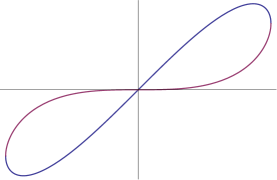
Figure 7.1. The spectral curve $\Sigma$ of (7.2). The horizontal line is the divisor $C_{\infty}$ at infinity, and the vertical line is the fiber class $F$. The spectral curve intersects with $C_{\infty}$ four times. One of the two curve germ components is given by $w=u$, and the other by $w=u^{3}$.

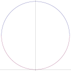
Figure 7.2. The desingularization $\widetilde{\Sigma}$ of the spectral curve (7.2).

The discriminant of the defining equation (7.2) is

$$\left(-\frac{1}{4}x^{2}+1\right)(dx)^{2}=-\frac{1}{4}(x-2)(x+2)(dx)^{2}=\frac{u^{2}-\frac{1}{4}}{u^{6}}(du)^{2}.$$

It has two simple zeros at $x=\pm 2$ and a pole of order $6$ at $x=\infty$. We note that

$${\text{\rm{tr}}}(\phi)=-xdx=\frac{du}{u^{3}}$$

has a cubic pole at $u=0$. As explained in Case 3 of the proof of Theorem 4.2, we need to compare the poles of ${\text{\rm{tr}}}(\phi)$ and

$$\det(\phi)=(dx)^{2}=\frac{(du)^{2}}{u^{4}}.$$

Since $4-3=1$, we blow up $\Sigma$ once at its nodal singularity $(u,w)=(0,0)$. We introduce $w=w_{1}u$. Then (7.3) becomes

(7.4) $$u^{2}+\left(w_{1}-{\frac{1}{2}}\right)^{2}=\frac{1}{4}.$$

The geometric genus formula (4.12) tells us that $\Sigma_{\min}$ has genus $0$, and $\Sigma_{\min}\longrightarrow C$ is ramified at two points, corresponding to the original ramification points $(x,y)=(\pm 2,\mp 1)$ of $\Sigma$. The rational parametrization of (7.4) is given by

$$\begin{cases}u={\frac{1}{2}}\cdot\frac{t^{2}-1}{t^{2}+1}\\ w_{1}={\frac{1}{2}}-\frac{t}{t^{2}+1},\end{cases}$$

where $t$ is an affine coordinate of $\widetilde{\Sigma}$ such that $t=\pm 1$ gives $(u,w)=(0,0)$. The parameter $t$ is a normalization coordinate of the spectral curve $\Sigma$:

(7.5) $$\begin{cases}x=2+\frac{4}{t^{2}+1}\\ y=-\frac{t+1}{t-1},\end{cases}\qquad\begin{cases}u={\frac{1}{2}}\cdot\frac{t^{2}-1}{t^{2}+1}\\ w=\frac{1}{4}\cdot\frac{(t-1)^{3}(t+1)}{(t^{2}+1)^{2}}.\end{cases}$$

We notice that the expression of (7.5) is exactly the same as [19, (3.13), (3.14)]. The integral topological recursion applied to $\widetilde{\Sigma}$ again agrees with that of [19].

The quantum curve construction of [46] is thus consistent with our new definition. The result is

(7.6) $$\left(\left(\hbar\frac{d}{dx}\right)^{2}+x\left(\hbar\frac{d}{dx}\right)+1\right)\Psi(x,\hbar)=0.$$

Since $x$ and $d/dx$ do not commute, the passage from (7.2) to (7.6) is non-trivial, in the sense that the constant term could have contained a term $c\cdot\hbar$. On the affine open subset $U_{1}={\mathbb{P}}^{1}\setminus\{0\}$, the operator of (7.6) has an expression

$$u^{4}\left(\hbar\frac{d}{du}\right)^{2}+(2u^{3}\hbar-u)\left(\hbar\frac{d}{du}\right)+1\in\widetilde{{\mathcal{D}}_{U_{1}}}.$$

Thus the point $\infty\in{\mathbb{P}}^{1}$ is an irregular singular point of class $2$ of (7.6) for $\hbar\neq 0$.

The semi-classical limit (6.14) of (7.6) using the WKB formula (1.8) is

(7.7) $$S_{0}^{\prime}(x)^{2}+xS_{0}^{\prime}(x)+1=0.$$

Following [19], define

(7.8) $$z=\frac{t+1}{t-1}=\sum_{m=0}^{\infty}\frac{C_{m}}{x^{2m+1}},$$

where $C_{m}=\frac{1}{m+1}\binom{2m}{m}$ is the $m$-th Catalan number. The inverse function of (7.8) for $x=\infty\Rightarrow z=0$ is given by $x=x(z)=z+\frac{1}{z}$. In terms of $z$, the two solutions of (7.7) are given by

(7.9) $$S_{0}\big{(}x(z)\big{)}=\begin{cases}-{\frac{1}{2}}z^{2}+\log z+{\text{\rm{const}}}\\ -{\frac{1}{2}}\frac{1}{z^{2}}-\log z+{\text{\rm{const}}}.\end{cases}$$

Corresponding to these choices, the solutions to the consistency condition (6.15) are given by

(7.10) $$S_{1}\big{(}x(z)\big{)}=\begin{cases}-{\frac{1}{2}}\log(1-z^{2})+{\text{\rm{const}}}\\ -{\frac{1}{2}}\log(1-z^{2})+\log z+{\text{\rm{const}}}.\end{cases}$$

Every solution of (7.6) is a linear combination of two solutions, with coefficients given by arbitrary functions in $\hbar$. One is given by the Kummer confluent hypergeomtric function of (1.24):

$$\Psi_{1}(x,\hbar)={}_{1}F_{1}\left(\frac{1}{2\hbar};{\frac{1}{2}};-\frac{x^{2}}{2\hbar}\right).$$

The other is a bit more complicated function known as the Tricomi confluent hypergeomtric function

(7.11) $$\Psi_{2}(x,\hbar)=\frac{\Gamma[{\frac{1}{2}}]}{\Gamma[\frac{1}{2\hbar}+{\frac{1}{2}}]}{}_{1}F_{1}\left(\frac{1}{2\hbar};{\frac{1}{2}};-\frac{x^{2}}{2\hbar}\right)+\frac{\Gamma[-{\frac{1}{2}}]}{\Gamma[\frac{1}{2\hbar}]}\sqrt{\frac{x^{2}}{-2\hbar}}{}_{1}F_{1}\left(\frac{1}{2\hbar}+{\frac{1}{2}};\frac{3}{2};-\frac{x^{2}}{2\hbar}\right).$$

For a positive real $\hbar>0$, let us consider a special solution

(7.12) $$\Psi^{{\text{\rm{Catalan}}}}(x,\hbar):=\left(-\frac{1}{2\hbar}\right)^{\frac{1}{2\hbar}}\Psi_{2}(x,\hbar).$$

This solution corresponds to the WKB solution (1.8) for the first choices of (7.9) and (7.10), with both constants of integration to be set $0$. Then we have a closed formula for the all-order asymptotics of this particular confluent hypergeometric function:

(7.13) $$\Psi^{{\text{\rm{Catalan}}}}(x,\hbar) =\left(\frac{1}{x}\right)^{\frac{1}{\hbar}}\sum_{n=0}^{\infty}\frac{\hbar^{n}\left(\frac{1}{\hbar}\right)_{2n}}{(2n)!!}\cdot\frac{1}{x^{2n}}$$

$$=\exp\left(\sum_{2g-2+n\geq-1}\frac{1}{n!}\hbar^{2g-2+n}F_{g,n}^{\text{\rm{Catalan}}}(x,\dots,x)\right),$$

where $(1/\hbar)_{2n}$ is the Pochhammer symbol (1.25). The free energies are defined by

(7.14) $$F_{g,n}^{\text{\rm{Catalan}}}(x_{1},\dots,x_{n})=\sum_{\mu_{1},\dots,\mu_{n}>0}\frac{C_{g,n}(\mu_{1},\dots,\mu_{n})}{\mu_{1}\cdots\mu_{n}}\prod_{i=1}^{n}x_{i}^{-\mu_{i}}$$

for $2g-2+n>0$, and $F_{0,1}^{\text{\rm{Catalan}}}(x)=S_{0}(x)$ and ${\frac{1}{2}}F_{0,2}^{\text{\rm{Catalan}}}(x)=S_{1}(x)$. Here, $C_{g,n}(\mu_{1},\dots,\mu_{n})$ is the generalized Catalan number of genus $g$ and $n$ labeled vertices of degrees $(\mu_{1},\dots,\mu_{n})$ that counts the number of cellular graphs [19, 48]. In [19, Theorem 4.3, Proposition A.1], we show that $F_{g,n}^{C}$ satisfies the differential recursion equation (6.11). (We note that the differential recursion of [19] is derived by taking the Laplace transform of [48, Equation 6]). The initial geometric data (1.7) are also the same as [19, (3.12), (4.3)]. Therefore, the application of the topological recursion to the desingularized spectral curve $\Sigma_{\min}$ produces (7.14), and the quantum curve (7.6).

At the special value $\hbar=1$, the expansion (7.13) has the following simple form

$$\sum_{n=0}^{\infty}\frac{(2n-1)!!}{x^{2n+1}}=\exp\left(\sum_{2g-2+n\geq-1}\frac{1}{n!}\sum_{\mu_{1},\dots,\mu_{n}>0}\frac{C_{g,n}(\mu_{1},\dots,\mu_{n})}{\mu_{1}\cdots\mu_{n}}\prod_{i=1}^{n}x^{-(\mu_{1}+\cdots+\mu_{n})}\right).$$

Note that the sum of the degrees of the vertices $\mu_{1}+\cdots+\mu_{n}$ is always even. Therefore, except for the unstable geometries $(g,n)=(0,1)$ and $(0,2)$, the above expansion is in $x^{-2}$. This indicates that the Hermite equation has an irregular singular point of class $2$ at $x=\infty$.

7.2. Gauß hypergeometric differential equation

The Higgs bundle $(E,\phi)$ on ${\mathbb{P}}^{1}$ is again given by the trivial bundle $E={\mathcal{O}}_{{\mathbb{P}}^{1}}\oplus{\mathcal{O}}_{{\mathbb{P}}^{1}}$, and a Higgs field

(7.15) $$\phi=\begin{bmatrix}&\frac{1}{x}\\ \\ -\frac{ab}{x-1}&-\frac{(a+b+1)x-c}{x(x-1)}\end{bmatrix}dx,$$

where $a,b,c$ are constant parameters. The spectral curve $\Sigma\in{\mathbb{F}}_{2}$ is defined by

(7.16) $$x(x-1)y^{2}+((a+b+1)x-c)y+ab=0.$$

In terms of the $(u,w)$ coordinate of (1.20), the spectral curve is given by

(7.17) $$abw^{2}+(cu-a-b)uw-u^{2}(u-1)=0.$$

It has an ordinary double point at $(u,w)=(0,0)$. The discriminant divisor of (4.7) is

(7.18) $$\Delta^{\text{\rm{Gau\ss}}}=\left(\frac{\left(\frac{1}{4}((a+b+1)x-1)^{2}-abx(x-1)\right)(dx)^{2}}{x^{2}(x-1)^{2}}\right),$$

which consists of two simple zeros and $3$ double poles at $x=0,1,\infty$. Following Definition 4.7, we blow up ${\mathbb{F}}_{2}$ once at the point at infinity of $\Sigma$ to construct the normalization $\Sigma_{\min}$. The invariant $\beta$ of (4.11) is equal to $2$, and hence $\Sigma_{\min}$ is isomorphic to ${\mathbb{P}}^{1}$.

The quantum curve we obtain is a Gauß hypergeometric differential equation

(7.19) $$\left(x(x-1)\left(\hbar\frac{d}{dx}\right)^{2}+\left((a+b+1)x-c\right)\hbar\frac{d}{dx}+ab\right)\Psi^{\text{\rm{Gau\ss}}}(x,\hbar)=0.$$

One of the two independent solutions that is holomorphic at $x=0$ is given in terms of a Gauß hypergeometric function

(7.20) $$\Psi^{\text{\rm{Gau\ss}}}(x,\hbar)={}_{2}F_{1}\Bigg{(}-\frac{\sqrt{\left(a+b+1-\hbar\right)^{2}-4ab}}{2\hbar}+\frac{a+b+1}{2\hbar}-\frac{1}{2},\\ \frac{\sqrt{\left(a+b+1-\hbar\right)^{2}-4ab}}{2\hbar}+\frac{a+b+1}{2\hbar}-\frac{1}{2};\frac{c}{\hbar};x\Bigg{)}.$$

If we choose $\sqrt{\left(a+b+1-\hbar\right)^{2}-4ab}=b-a$ when $\hbar=1$, then

(7.21) $$\Psi^{\text{\rm{Gau\ss}}}(x,1)={}_{2}F_{1}(a,b;c,x)=\sum_{n=0}^{\infty}\frac{(a)_{n}(b)_{n}}{(c)_{n}}\;\frac{x^{n}}{n!}$$

solves the standard form of the Gauß hypergeometric equation

(7.22) $$\left(x(x-1)\left(\frac{d}{dx}\right)^{2}+\left((a+b+1)x-c\right)\frac{d}{dx}+ab\right)\Psi^{\text{\rm{Gau\ss}}}(x,1)=0.$$

Now let us specialize $a=b={\frac{1}{2}},c=1$. We have the relation between the hypergeometric function and the period function of (1.11):

(7.23) $$\frac{\omega_{1}(x)}{\pi}={}_{2}F_{1}\left({\frac{1}{2}},{\frac{1}{2}};1,x\right).$$

The spectral curve (7.16) becomes

(7.24) $$x(x-1)y^{2}+(2x-1)y+\frac{1}{4}=0.$$

On the normalization $\widetilde{\Sigma}$, we have $W_{0,1}(x)=ydx$, which actually depends of the sheet of the covering $\tilde{\pi}:\widetilde{\Sigma}\longrightarrow{\mathbb{P}}^{1}$. For our purpose, we choose

(7.25) $$y=y(x)=\frac{-(2x-1)-\sqrt{3x^{2}-3x+1}}{2x\left(x-1\right)}.$$

Then

(7.26) $$S_{0}(x)=F_{0,1}(x)=\int y(x)dx\\ =\frac{x}{4}-\frac{21\left(4\sqrt{3}-7\right)}{32\left(2\sqrt{3}-3\right)^{2}}x^{2}+\frac{23\left(26\sqrt{3}-45\right)}{32\left(2\sqrt{3}-3\right)^{3}}x^{3}-\frac{2547\left(56\sqrt{3}-97\right)}{1024\left(2\sqrt{3}-3\right)^{4}}x^{4}\\ +\frac{7281\left(362\sqrt{3}-627\right)}{2560\left(2\sqrt{3}-3\right)^{5}}x^{5}-\frac{38115\left(780\sqrt{3}-1351\right)}{4096\left(2\sqrt{3}-3\right)^{6}}x^{6}+\frac{265869\left(5042\sqrt{3}-8733\right)}{28672\left(2\sqrt{3}-3\right)^{7}}x^{7}+\cdots$$

solves the semi-classical limit equation (6.14). The solution of the consistency condition (6.15) is given by

(7.27) $$S_{1}(x)=-\int\frac{y^{\prime}(x)}{2y(x)+\frac{2x-1}{x(x-1)}}dx\\ =-\frac{7}{32}x^{2}-\frac{53}{96}x^{3}-\frac{1075}{1024}x^{4}-\frac{4319}{2560}x^{5}-\frac{28319}{12288}x^{6}-\frac{72109}{28672}x^{7}+\cdots.$$

The solution of (6.16) for $m=1$ is

(7.28) $$S_{2}(x)=\frac{7x^{2}}{32}+\frac{113x^{3}}{96}+\frac{1821x^{4}}{512}+\frac{1269x^{5}}{160}+\frac{56151x^{6}}{4096}+\frac{487323x^{7}}{28672}+\cdots.$$

From (7.26), (7.27) and (7.28), we have an expression

(7.29) $$\exp\left(\frac{1}{\hbar}S_{0}(x)+S_{1}(x)+\hbar S_{2}(x)\right)\\ =1+\frac{x}{4\hbar}+\frac{1+7\hbar-7\hbar^{2}+7\hbar^{3}}{32\hbar^{2}}x^{2}+\frac{1+21\hbar+71\hbar^{2}-191\hbar^{3}+\cdots}{384\hbar^{3}}x^{3}\\ +\frac{1+42\hbar+473\hbar^{2}+598\hbar^{3}+\cdots}{6144\hbar^{4}}x^{4}+\frac{1+70\hbar+1585\hbar^{2}+1141-\hbar^{3}+\cdots}{122880\hbar^{5}}x^{5}+\cdots.$$

This is in good agreement of the hypergeometric function of (7.20), which can be expanded as

$$\Psi^{\text{\rm{Gau\ss}}}(x,\hbar)=1+\sum_{n=1}^{\infty}\frac{1}{4^{n}n!}\frac{\prod_{m=1}^{n}\left(1+8(m-1)\hbar+4(m-1)(m-2)\hbar^{2}\right)}{\prod_{m=1}^{n}\left(1+(m-1)\hbar\right)}\left(\frac{x}{\hbar}\right)^{n}\\ =1+\frac{x}{4\hbar}+\frac{1+8\hbar}{32\hbar(1+\hbar)}x^{2}+\frac{(1+8\hbar)(1+16\hbar+8\hbar^{2})}{384\hbar^{3}(1+\hbar)(1+2\hbar)}x^{3}\\ +\frac{(1+8\hbar)(1+16\hbar+8\hbar^{2})(1+24\hbar+24\hbar^{2})}{6144\hbar^{4}(1+\hbar)(1+2\hbar)(1+3\hbar)}x^{4}+\cdots,$$

up to order of $\hbar^{3}$ of the numerator of every coefficient of $x^{n}$, $n\geq 0$. The topological recursion applied to the spectral curve (7.16) with $F_{0,1}=S_{0}(x)$ and the standard Riemann prime form on $\widetilde{\Sigma}={\mathbb{P}}^{1}$ for $F_{0,2}$ then gives a genus expansion of $\Psi^{\text{\rm{Gau\ss}}}(x,\hbar)$, constructing a genus $g$ B-model on the curve (7.16).

Acknowledgement.

The authors are grateful to the American Institute of Mathematics in Palo Alto, the Banff International Research Station, the Institute for Mathematical Sciences at the National University of Singapore, Kobe University, and Max-Planck-Institut für Mathematik in Bonn, for their hospitality and financial support. A large portion of this work is carried out during the authors’ stay in these institutions. They also thank Jørgen Andersen, Philip Boalch, Leonid Chekhov, Bertrand Eynard, Tamás Hausel, Kohei Iwaki, Maxim Kontsevich, Alexei Oblomkov, Albert Schwarz, Yan Soibelman, Ruifang Song, and Peter Zograf for useful comments, suggestions, and discussions. M.M. thanks the Euler International Mathematical Institute in St. Petersburg for hospitality, where the paper is completed. The research of O.D. has been supported by GRK 1463 Analysis, Geometry, and String Theory at the Leibniz Universität Hannover. The research of M.M. has been supported by MPIM in Bonn, NSF grants DMS-1104734 and DMS-1309298, and NSF-RNMS: Geometric Structures And Representation Varieties (GEAR Network, DMS-1107452, 1107263, 1107367).

References

- [1] M. Aganagic, R. Dijkgraaf, A. Klemm, M. Mariño, and C. Vafa, Topological Strings and Integrable Hierarchies, [arXiv:hep-th/0312085], Commun. Math. Phys. 261, 451–516 (2006).
- [2] J.E. Andersen, L.O Chekhov, P. Norbury, and R.C. Penner, Cohomological field theories, discretisation of moduli spaces, and Gaussian means, Private communication.
- [3] D. Arinkin, On -connections on a curve where is a formal parameter, Mathematical Research Letters 12, 551–565 (2005).
- [4] O. Biquard and P. Boalch, Wild non-Abelian Hodge theory on curves, Compos. Math. 140, 179–204 (2004).
- [5] P. Boalch, Symplectic manifolds and isomonodromic deformations, Adv. in Math. 163, 137–205 (2001).
- [6] P. Boalch, Hyperkähler manifolds and nonabelian Hodge theory of (irregular) curves, arXiv:1203.6607v1 (2012).
- [7] V. Bouchard and B. Eynard, Think globally, compute locally, JHEP 02, Article: 143 (34 pages), (2013).
- [8] V. Bouchard, D. Hernández Serrano, X. Liu, and M. Mulase, Mirror symmetry for orbifold Hurwitz numbers, arXiv:1301.4871 [math.AG] (2013).
- [9] V. Bouchard, A. Klemm, M. Mariño, and S. Pasquetti, Remodeling the B-model, Commun. Math. Phys. 287, 117–178 (2009).
- [10] V. Bouchard, A. Klemm, M. Mariño, and S. Pasquetti, Topological open strings on orbifolds, Commun. Math. Phys. 296, 589–623 (2010).
- [11] L. Chekhov, B. Eynard, and N. Orantin, Free energy topological expansion for the -matrix model, Journal of High Energy Physics 0612:053 (2006).
- [12] R. Dijkgraaf, H. Fuji, and M. Manabe, The Volume Conjecture, Perturbative Knot Invariants, and Recursion Relations for Topological Strings, Nucl. Phys. B849,166–211 (2011).
- [13] R. Dijkgraaf, L. Hollands, and P. Sułkowski, Quantum curves and -modules, Journal of High Energy Physics 0810.4157, 1–58 (2009).
- [14] R. Dijkgraaf, L. Hollands P. Sułkowski, and C. Vafa, Supersymmetric gauge theories, intersecting branes and free Fermions, Journal of High Energy Physics 0802.106, (2008).
- [15] R. Dijkgraaf, E. Verlinde, and H. Verlinde, Loop equations and Virasoro constraints in non-perturbative two-dimensional quantum gravity, Nucl. Phys. B348, 435–456 (1991).
- [16] N. Do and D. Manescu, Quantum curves for the enumeration of ribbon graphs and hypermaps, arXiv:1312.6869 [math.GT] (2013).
- [17] B. Dubrovin, Geometry of 2d topological field theories, arxiv:hep-th/9407018 [physics.hep-th] (1994).
- [18] O. Dumitrescu and M. Mulase, Quantum curves for Hitchin fibrations and the Eynard-Orantin theory, Lett. Math. Phys. 104, 635–671 (2014).
- [19] O. Dumitrescu, M. Mulase, A. Sorkin and B. Safnuk, The spectral curve of the Eynard-Orantin recursion via the Laplace transform, in “Algebraic and Geometric Aspects of Integrable Systems and Random Matrices,” Dzhamay, Maruno and Pierce, Eds. Contemporary Mathematics 593, 263–315 (2013).
- [20] P. Dunin-Barkowski, M. Mulase, P. Norbury, A. Popolitov, and S. Shadrin, Quantum spectral curve for the Gromov-Witten theory of the complex projective line, arXiv:1312.5336 [math-ph] (2013).
- [21] B. Eynard, All genus correlation functions for the hermitian 1-matrix model, Journal of High Energy Physics 0411:031 (2004).
- [22] B. Eynard, Intersection numbers of spectral curves, arXiv:1104.0176 (2011).
- [23] B. Eynard, M. Mulase and B. Safnuk, The Laplace transform of the cut-and-join equation and the Bouchard-Mariño conjecture on Hurwitz numbers, Publications of the Research Institute for Mathematical Sciences 47, 629–670 (2011).
- [24] B. Eynard and N. Orantin, Invariants of algebraic curves and topological expansion, Communications in Number Theory and Physics 1, 347–452 (2007).
- [25] B. Eynard and N. Orantin, Computation of open Gromov-Witten invariants for toric Calabi-Yau 3-folds by topological recursion, a proof of the BKMP conjecture, arXiv:1205.1103v2 [math-ph] (2013).
- [26] B. Fang, C.-C. M. Liu, and Z. Zong, All genus open-closed mirror symmetry for affine toric Calabi-Yau 3-orbifolds, arXiv:1310.4818 [math.AG] (2013).
- [27] S. Garoufalidis, On the characteristic and deformation varieties of a knot, Geometry & Topology Monographs 7, 291–309 (2004).
- [28] S. Garoufalidis and T.T.Q. Lê, The colored Jones function is q holonomic, Geometry and Topology 9, 1253–1293 (2005).
- [29] V. Ginzburg, Lectures on -modules, Lectures delivered at the University of Chicago, Winter 1998, with collaboration of V. Baranovsky and S. Evens (1998).
- [30] S. Gukov and P. Sułkowski, A-polynomial, B-model, and quantization, arXiv:1108.0002v1 [hep-th] (2011).
- [31] R. Hartshorne, Algebraic geometry, Springer, New York 1977.
- [32] N.J. Hitchin, The self-duality equations on a Riemann surface, Proc. London Math. Soc. (Ser. 3) 55, 59–126 (1987).
- [33] N.J. Hitchin, Stable bundles and integrable systems, Duke Math. J. 54, 91–114 (1987).
- [34] A. Hodge and M. Mulase, Hitchin integrable systems, deformations of spectral curves, and KP-type equations, Advanced Studies in Pure Mathematics 59, 31–77 (2010).
- [35] L. Hollands, Topological strings and quantum curves, Ph.D. Thesis, University of Amsterdam arXiv:0911.3413 [hep-th] (2009).
- [36] D. Huybrechts and M. Lehn, Stable pairs on curves and surfaces, arXiv:alg-geom/9211001 (1992).
- [37] A. Kapustin and E. Witten, Electric-magnetic duality and the geometric Langlands program, Communications in Number Theory and Physics 1, 1–236 (2007).
- [38] M. Kontsevich, Intersection theory on the moduli space of curves and the matrix Airy function, Communications in Mathematical Physics 147, 1–23 (1992).
- [39] M. Kontsevich and Y. Soibelman, Wall-crossing structures in Donaldson-Thomas invariants, integrable systems and Mirror Symmetry, arXiv:1303.3253 [math.AG] (2013).
- [40] M. Kontsevich and D. Zagier, Periods, in “ Mathematics unlimited–2001 and beyond”, 771–808, Springer-verlag, Berlin, (2001).
- [41] Ph. Maisonobe and C. Sabbah, Aspects of the theory of -modules, Kaiserslautern Lecture Notes (2002).
- [42] Yu.I. Manin, Algebraic curves over fields with differentiation, Izvestiya Akademii Nauk SSSR, Seriya Matematicheskaya (in Russian) 22, 737–756 (1958).
- [43] M. Mariño, Open string amplitudes and large order behavior in topological string theory, J. High Energy Physics 0803-060, 1–33 (2008).
- [44] M. Mulase and M. Penkava, Topological recursion for the Poincaré polynomial of the combinatorial moduli space of curves, Advances in Mathematics 230, 1322–1339 (2012).
- [45] M. Mulase, S. Shadrin, and L. Spitz, The spectral curve and the Schrödinger equation of double Hurwitz numbers and higher spin structures, Communications in Number Theory and Physics 7, 1–19 (2013).
- [46] M. Mulase and P. Sułkowski, Spectral curves and the Schrödinger equations for the Eynard-Orantin recursion, arXiv:1210.3006 (2012).
- [47] M. Mulase and N. Zhang, Polynomial recursion formula for linear Hodge integrals, Communications in Number Theory and Physics 4, 267–294 (2010).
- [48] T.R.S. Walsh and A.B. Lehman, Counting rooted maps by genus. I, Journal of Combinatorial Theory B-13, 192–218 (1972).
- [49] E. Witten, Two dimensional gravity and intersection theory on moduli space, Surveys in Differential Geometry 1, 243–310 (1991).
- [50] E. Witten, Gauge theory and wild ramification, Analysis and Applications 6, 429–501 (2008).
- [51] E. Witten, Mirror symmetrym Hitchin’s equations, and Langlands duality, arXiv:0802.0999 (2008).
- [52] E. Witten, Analytic continuation of Chern-Simons theory, arXiv:1001.2933v4 [hep-th] (2010).
- [53] J. Zhou, Intersection numbers on Deligne-Mumford moduli spaces and quantum Airy curve, arXiv:1206.5896 [math.AG] (2012).
- [54] J. Zhou, Quantum Mirror Curves for and the Resolved Confiold, arXiv:1207.0598v1 [math.AG] (2012).