Convergence Analysis for Regular Wireless Consensus Networks

Sateeshkrishna Dhuli, Kumar Gaurav, and Y.N.Singh
Abstract

Average consensus algorithms can be implemented over wireless sensor networks (WSN), where global statistics can be computed using communications among sensor nodes locally. Simple execution, robustness to global topology changes due to frequent node failures and underlying distributed philosophy have made consensus algorithms more suitable to WSNs. Since these algorithms are iterative in nature, it is very difficult to predict the convergence time of the average consensus algorithm on WSNs. We study the convergence of the average consensus algorithms for WSNs using distance regular graphs. We have obtained the analytical expressions for optimal consensus parameter and optimal convergence parameter which estimates the convergence time for r๐‘Ÿr-nearest neighbor cycle and torus networks. We have also derived the generalized expression for optimal consensus parameter and optimal convergence parameter for m๐‘šm-dimensional r๐‘Ÿr-nearest neighbor torus networks. The obtained analytical results agree with the simulation results and shown the effect of network dimension, number of nodes and nearest neighbors on convergence time. This work provides the basic analytical tools for managing and controlling the performance of average consensus algorithms over finite sized practical WSNs.

Index Terms:
Consensus networks, WSNs, Average consensus algorithms, r๐‘Ÿr-nearest neighbor networks, Convergence time

I Introduction

Consensus algorithms have received a lot of attention due to their ability to compute the desired global statistics by exchanging information only with direct neighbors. Average consensus algorithms have been extensively studied in distributed agreement and synchronization problems in the multi agent systems and load balancing in parallel computers ( [1], [2], [3]). In contrast to centralized algorithms, the underlying distributed and decentralized philosophy avoids the need of any central fusion for collecting the information. This approach is particularly suitable in the following situations: 1) global network topology information is not known; 2) dynamic topology changes because of frequent node failures; 3) the nodes are computationally constrained and incapable to support the sophisticated routing techniques.

Distributed average consensus algorithms can be applied to WSNs for data fusion [4], [5], [6]. As the consensus algorithms are iterative in nature, convergence rate of the algorithms greatly influences the performance of the WSNs and it is lower bounded by the second smallest eigenvalue of the graph Laplacian [7]. To make this algorithm useful in a sensor network context, it is necessary to maximize the convergence rate to reach the consensus as soon as possible. Thus, extensive studies to increase the convergence rate have been done in the literature. In [8], distributed average consensus has been considered when the topology is random and the communication in the channels is corrupted by additive noise. It was proved that running the consensus for long time reduces the bias of the final average estimate but increases its variance. A closed form expression for the mean square error of the state and the optimum choice of parameters have been derived in [9] to guarantee the fastest convergence. Consensus on small world and ramanujan networks has been studied in [10], [11] and it has been proved that convergence rate is maximized for these topologies. Optimal topology framework which increases the convergence rate and minimizes the energy consumption has been studied in [12]. In our work, we study the convergence of the consensus algorithm for finite distance-regular networks with varying number of nearest neighbors. These finite sized networks represent the notion of geographical proximity in the practical WSNs. The main motivation for using the regular graph model is that most of the practical WSNs are finite sized which cannot be studied by asymptotic results existing in the literature. Random geometric graphs that model WSNs have similar asymptotic behavior as regular graph [13], which are convenient to analyze the wireless networks [14], [15], [16]. Our results are more precise and can be applied to most of the practical WSNs. In r๐‘Ÿr-nearest neighbor cycle and torus, an edge exists between every pair of neighbors that are r๐‘Ÿr hops away. If a nodeโ€™s transmission radius is increased, it will able to communicate with more number of nodes. Similarly, overhead increases with the number of nearest neighbors. So, we can consider the variable r๐‘Ÿr as both transmission radius and node overhead in WSNs. Effect of communication parameters on consensus algorithmโ€™s convergence rate has been studied analytically in [17]. But it does not provide the exact formulation of the convergence time for average consensus algorithms. Despite the fact that distributed average consensus is simple to implement, it is generally difficult to predict its convergence time. Although there have been several studies of wireless consensus networks, analytical tools to control the network performance for WSNs are still inadequate. In this paper, we derive the generalized expressions to efficiently and exactly compute the optimal convergence, consensus parameter to estimate the convergence time for finite WSNs. This kind of analysis helps in estimating the convergence time efficiently as it avoids usage of computationally expensive algorithms which depends on thousands of simulation trails.

In summary, the paper is organized as follows. In Section II, we have given brief review of the consensus algorithms. In Section III, we have discussed the r๐‘Ÿr-nearest neighbor networks and derived the generalized eigenvalue expressions of weight matrix for the m๐‘šm-dimensional WSNs. Analytical expressions for optimal consensus and optimal convergence parameters have been derived in Section IV. Finally, in Section V, simulation results have been presented and compared with the obtained analytical results.

II Review of consensus algorithms

Let G=(V,E)๐บ๐‘‰๐ธG=(V,E), be an undirected graph with node set V={1,2,โ€ฆโ€‹โ€ฆโ€‹n}๐‘‰12โ€ฆโ€ฆ๐‘›V=\left\{{1,2,......n}\right\} and an edge set EโŠ†Vร—V๐ธ๐‘‰๐‘‰E\subseteq V\times V. And, let A๐ดA be the nร—n๐‘›๐‘›n\times n symmetric adjacency matrix of the graph G๐บG, where each entry of adjacency matrix is represented by aiโ€‹jsubscript๐‘Ž๐‘–๐‘—a_{ij}, which is 111 if node i๐‘–i is connected to node j๐‘—j, else it is 00. The degree matrix D๐ทD is defined as the diagonal matrix whose entry is diโ€‹i=degโก(vi)subscript๐‘‘๐‘–๐‘–degreesubscript๐‘ฃ๐‘–d_{ii}=\deg(v_{i}), where dโ€‹eโ€‹gโ€‹(ฮฝi)=โˆ‘j=1naiโ€‹j=โˆ‘j=1najโ€‹i๐‘‘๐‘’๐‘”subscript๐œˆ๐‘–superscriptsubscript๐‘—1๐‘›subscript๐‘Ž๐‘–๐‘—superscriptsubscript๐‘—1๐‘›subscript๐‘Ž๐‘—๐‘–deg(\nu_{i})=\sum_{j=1}^{n}a_{ij}=\sum_{j=1}^{n}a_{ji}. The Laplacian matrix of the graph G๐บG is nร—n๐‘›๐‘›n\times n symmetric matrix L=Dโˆ’A๐ฟ๐ท๐ดL=D-A, whose entries are

liโ€‹j=ljโ€‹i={degโก(vi)โ€‹iโ€‹fโ€‹j=i,โˆ’aiโ€‹jiโ€‹fโ€‹jโ‰ i.subscript๐‘™๐‘–๐‘—subscript๐‘™๐‘—๐‘–casesdegreesubscript๐‘ฃ๐‘–๐‘–๐‘“๐‘—๐‘–subscript๐‘Ž๐‘–๐‘—๐‘–๐‘“๐‘—๐‘–l_{ij}=l_{ji}=\left\{\begin{array}[]{l}\deg(v_{i})\,\,\,if\,\,j=i,\\ -a_{ij}\,\,\,\,\,\,\,\,\,if\,\,j\neq\,i.\\ \end{array}\right. (1)

The Laplacian is a positive definite matrix, hence the eigenvalues are given by

0=ฮป1(L)โ‰คฮป2(L)โ‰คฮป3(L)โ€ฆโ€ฆโ€ฆ.โ‰คฮปN(L).0=\lambda_{1}\left(L\right)\leq\lambda_{2}\left(L\right)\leq\lambda_{3}\left(L\right)..........\leq\lambda_{N}\left(L\right). (2)

The graph topology is connected only if its zero eigenvalue has multiplicity one. The second smallest eigenvalue ฮป2โ€‹(L)>0subscript๐œ†2๐ฟ0\lambda_{2}\left(L\right)>0 is the algebraic connectivity or the fiedler value [7] of the network.

Let xiโ€‹(0)subscript๐‘ฅ๐‘–0x_{i}(0) be the real scalar assigned to the node i๐‘–i at t=0๐‘ก0t=0. Average consensus algorithm computes the average xaโ€‹vโ€‹g=โˆ‘i=1nxiโ€‹(0)nsubscript๐‘ฅ๐‘Ž๐‘ฃ๐‘”superscriptsubscript๐‘–1๐‘›subscript๐‘ฅ๐‘–0๐‘›x_{avg}=\frac{{\sum\nolimits_{i=1}^{n}{x_{i}(0)}}}{n} at every node through a decentralized approach which does not require the sink node/base station. The minimization of disagreement between the xiโ€‹(0)subscript๐‘ฅ๐‘–0x_{i}(0) of the interacting nodes is expressed as a quadratic form [18] on Laplacian.

Jโ€‹(x):=14โ€‹โˆ‘i=1nโˆ‘jโ€‹ฯตโ€‹Nin(xiโˆ’xj)2,=14โ€‹โˆ‘i=1nโˆ‘jโ€‹ฯตโ€‹Ninaiโ€‹jโ€‹(xiโˆ’xj)2,=12โ€‹xTโ€‹Lโ€‹x.assign๐ฝ๐‘ฅ14superscriptsubscript๐‘–1๐‘›superscriptsubscript๐‘—italic-ฯตsubscript๐‘๐‘–๐‘›superscriptsubscript๐‘ฅ๐‘–subscript๐‘ฅ๐‘—2absent14superscriptsubscript๐‘–1๐‘›superscriptsubscript๐‘—italic-ฯตsubscript๐‘๐‘–๐‘›subscript๐‘Ž๐‘–๐‘—superscriptsubscript๐‘ฅ๐‘–subscript๐‘ฅ๐‘—2absent12superscript๐‘ฅ๐‘‡๐ฟ๐‘ฅ\begin{array}[]{l}J(x):=\frac{1}{4}\sum_{i=1}^{n}\sum_{j\epsilon N_{i}}^{n}(x_{i}-x_{j})^{2},\\ \,\,\,\,\,\,\,\,\,\,\,\,\,\,\,\,=\frac{1}{4}\sum_{i=1}^{n}\sum_{j\epsilon N_{i}}^{n}a_{ij}(x_{i}-x_{j})^{2},\\ \,\,\,\,\,\,\,\,\,\,\,\,\,\,\,\,=\frac{1}{2}x^{T}Lx.\end{array} (3)

The quadratic form in (3) is achieved using a simple steepest descent technique, and the minimum of (3) updated by the [3] following expression.

xห™โ€‹(t)=โˆ’Lโ€‹xโ€‹(t).ห™๐‘ฅ๐‘ก๐ฟ๐‘ฅ๐‘ก\dot{x}(t)=-Lx(t). (4)

where xห™โ€‹(t)ห™๐‘ฅ๐‘ก\dot{x}(t) denotes the average of all the real scalar values.

At each step, node i๐‘–i carries out its update based on its local state and communication with itโ€™s direct neighbors.

xiโ€‹(t+1)=xiโ€‹(t)+hโ€‹โˆ‘jโˆˆNi(xjโ€‹(t)โˆ’xiโ€‹(t)),i=1,โ€ฆ,n,formulae-sequencesubscript๐‘ฅ๐‘–๐‘ก1subscript๐‘ฅ๐‘–๐‘กโ„Žsubscript๐‘—subscript๐‘๐‘–subscript๐‘ฅ๐‘—๐‘กsubscript๐‘ฅ๐‘–๐‘ก๐‘–1โ€ฆ๐‘›x_{i}(t+1)=x_{i}(t)+h\sum\limits_{j\in N_{i}}{(x_{j}(t)-x_{i}(t))},\,\,\,i=1,...,n, (5)

where hโ„Žh is a consensus parameter and Nisubscript๐‘๐‘–N_{i} denotes neighbor set of node i๐‘–i. This iterative method is expressed as the simple linear iteration

xโ€‹(t+1)=Wโ€‹xโ€‹(t),t=0,1,2โ€‹โ€ฆ,formulae-sequence๐‘ฅ๐‘ก1๐‘Š๐‘ฅ๐‘ก๐‘ก012โ€ฆx(t+1)=Wx(t),\,\,\,\,t=0,1,2..., (6)

where W๐‘ŠW denotes weight matrix, and Wiโ€‹jsubscript๐‘Š๐‘–๐‘—W_{ij} is a weight associated with the edge (i,j)๐‘–๐‘—(i,j). If we assign equal weight hโ„Žh to each link in the network, then from [19], optimal weight for a given topology is

Wiโ€‹j={hiโ€‹f,(i,j)โˆˆE,1โˆ’hโ€‹dโ€‹eโ€‹gโ€‹(ฮฝi)iโ€‹f,i=j,0oโ€‹tโ€‹hโ€‹eโ€‹rโ€‹wโ€‹iโ€‹sโ€‹e.W_{ij}=\left\{\begin{matrix}h&if,\,\,\,\,(i,j)\in E,\\ 1-hdeg(\nu_{i})&if,\,\,\,\,i=j,\\ 0&otherwise.\end{matrix}\right. (7)

where optimal link weight or consensus parameter [19] is defined as

h=2ฮป2โ€‹(L)+ฮปnโ€‹(L).โ„Ž2subscript๐œ†2๐ฟsubscript๐œ†๐‘›๐ฟh=\frac{2}{{\lambda_{2}(L)+\lambda_{n}(L)}}. (8)

and Weight matrix is given by

W=Iโˆ’hโ€‹L.๐‘Š๐ผโ„Ž๐ฟW=I-hL. (9)

where I๐ผI is a nร—n๐‘›๐‘›n\times n identity matrix. Let ฮปnโ€‹(W)subscript๐œ†๐‘›๐‘Š\lambda_{n}(W) be the ntโ€‹hsuperscript๐‘›๐‘กโ„Žn^{th} eigenvalue of W๐‘ŠW, then ฮปnโ€‹(W)=1โˆ’hโ€‹ฮปnโ€‹(L)subscript๐œ†๐‘›๐‘Š1โ„Žsubscript๐œ†๐‘›๐ฟ\lambda_{n}(W)=1-h\lambda_{n}(L) satisfies

1=ฮป1โ€‹(W)>ฮป2โ€‹(W)>ฮป3โ€‹(W)โ€‹โ€ฆโ€‹โ€ฆโ€‹โ€ฆโ€‹ฮปnโ€‹(W).1subscript๐œ†1๐‘Šsubscript๐œ†2๐‘Šsubscript๐œ†3๐‘Šโ€ฆโ€ฆโ€ฆsubscript๐œ†๐‘›๐‘Š1=\lambda_{1}(W)>\lambda_{2}(W)>\lambda_{3}(W).........\lambda_{n}(W). (10)

From (6) convergence rate is expressed as

โ€–xiโˆ’xaโ€‹vโ€‹gโ€–โ‰คโ€–xโ€‹(0)โˆ’xaโ€‹vโ€‹gโ€–โ€‹ฮณi,normsubscript๐‘ฅ๐‘–subscript๐‘ฅ๐‘Ž๐‘ฃ๐‘”norm๐‘ฅ0subscript๐‘ฅ๐‘Ž๐‘ฃ๐‘”superscript๐›พ๐‘–\left\|x_{i}-x_{avg}\right\|\leq\left\|x(0)-x_{avg}\right\|\gamma^{i}, (11)

where convergence parameter (ฮณ๐›พ\gamma) is

ฮณ=ฮปnโ€‹(L)โˆ’ฮป2โ€‹(L)ฮปnโ€‹(L)+ฮป2โ€‹(L).๐›พsubscript๐œ†๐‘›๐ฟsubscript๐œ†2๐ฟsubscript๐œ†๐‘›๐ฟsubscript๐œ†2๐ฟ\gamma=\frac{\lambda_{n}(L)-\lambda_{2}(L)}{\lambda_{n}(L)+\lambda_{2}(L)}. (12)

III r๐‘Ÿr-nearest neighbor networks

Multi-dimensional geometric wireless network topologies can be represented by r๐‘Ÿr-nearest neighbor networks [14], where nodes in the distance r๐‘Ÿr gets connected. The variable r๐‘Ÿr models the nodeโ€™s transmission radius or node overhead. These networks are one particular class of distance regular networks, where r๐‘Ÿr-nearest neighbor cycle and r๐‘Ÿr-nearest neighbor torus represents one dimensional and two dimensional topologies respectively.

III-A r๐‘Ÿr-nearest neighbor cycle

The r๐‘Ÿr-nearest cycle can be represented by a circulant matrix [20], and it is given by

[a1a2โ€ฆโ€ฆ..anโˆ’1ananโ€‹a1โ€‹โ€ฆ.โ€ฆ.anโˆ’2โ€‹anโˆ’1........a3a4โ€ฆโ€ฆโ€ฆ..a1a2a2โ€‹a3โ€‹โ€ฆโ€‹โ€ฆโ€‹โ€ฆโ€‹โ€ฆ.anโ€‹a1].\left[\begin{array}[]{l}a_{1}\,\,a_{2}\,\,........a_{n-1}\,\,a_{n}\\ a_{n}\,\,a_{1}\,\,....\,....a_{n-2}\,a_{n-1}\\ .\,\,\,\,\,\,\,.\,\,\,\,\,\,\,\,\,\,\,\,\,\,\,\,\,\,\,\,\,\,\,\,.\,\,\,\,\,\,\,\,\,.\\ .\,\,\,\,\,\,\,.\,\,\,\,\,\,\,\,\,\,\,\,\,\,\,\,\,\,\,\,\,\,\,\,.\,\,\,\,\,\,\,\,\,.\\ a_{3}\,\,a_{4}\,\,\,...........a_{1}\,\,\,a_{2}\\ a_{2}\,\,a_{3}\,\,.............a_{n}\,\,a_{1}\\ \end{array}\right]. (13)

where aisubscript๐‘Ž๐‘–a_{i}, i=1๐‘–1i=1 to n๐‘›n represents the topology coefficients. The ktโ€‹hsuperscript๐‘˜๐‘กโ„Žk^{th} eigenvalue of a circulant matrix is defined as

ฮปk=a1+a2ฯ‰k+โ€ฆโ€ฆโ€ฆโ€ฆ..+anฯ‰(nโˆ’1)โ€‹k.\lambda_{k}=a_{1}+a_{2}\omega^{k}+..............+a_{n}\omega^{(n-1)k}. (14)

where ฯ‰๐œ”\omega is the ntโ€‹hsuperscript๐‘›๐‘กโ„Žn^{th} root of 1, given by

ฯ‰=cosโก(2โ€‹ฯ€n)+zโ€‹sinโก(2โ€‹ฯ€n)=e2โ€‹ฯ€โ€‹zn.๐œ”2๐œ‹๐‘›๐‘ง2๐œ‹๐‘›superscript๐‘’2๐œ‹๐‘ง๐‘›\omega=\cos\left({\frac{{2\pi}}{n}}\right)+z\sin\left({\frac{{2\pi}}{n}}\right)=e^{\frac{2\pi z}{n}}. (15)

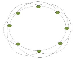
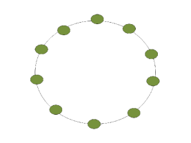
The 1-nearest cycle and 2-nearest cycle are shown in Fig. 1 and Fig. 2 respectively. Then adjacency matrix (A๐ดA) of a 1-nearest cycle is

A=[0โ€‰โ€‰1โ€‰โ€‰0โ€‹โ€ฆโ€‹โ€ฆโ€‹โ€ฆโ€‹โ€ฆโ€‹..0โ€‰โ€‰11โ€‰โ€‰0โ€‰โ€‰1โ€‹โ€ฆโ€‹โ€ฆโ€‹โ€ฆโ€‹โ€ฆโ€‹..0โ€‰0..........0โ€‰โ€‰0โ€‰โ€‰0โ€‹โ€ฆโ€‹โ€ฆโ€‹โ€ฆโ€‹โ€ฆโ€‹..0โ€‰โ€‰11โ€‰โ€‰0โ€‰โ€‰0โ€‹โ€ฆโ€‹โ€ฆโ€‹โ€ฆโ€‹โ€ฆโ€‹..1โ€‰0],๐ดdelimited-[]010โ€ฆโ€ฆโ€ฆโ€ฆ..01101โ€ฆโ€ฆโ€ฆโ€ฆ..00absentabsent000โ€ฆโ€ฆโ€ฆโ€ฆ..01100โ€ฆโ€ฆโ€ฆโ€ฆ..10A=\left[\begin{array}[]{l}0\,\,1\,\,0\,\,..............0\,\,1\\ 1\,\,0\,\,1\,\,..............0\,0\\ .\,\,\,\,.\,\,\,\,.\,\,\,\,\,\,\,\,\,\,\,\,\,\,\,\,\,\,\,\,\,\,\,\,\,.\,\,\,.\\ .\,\,\,\,.\,\,\,\,.\,\,\,\,\,\,\,\,\,\,\,\,\,\,\,\,\,\,\,\,\,\,\,\,\,.\,\,\,.\\ 0\,\,0\,\,0\,\,..............0\,\,1\\ 1\,\,0\,\,0\,\,..............1\,0\\ \end{array}\right], (16)

and degree matrix (D๐ทD) of a 1-nearest cycle is expressed as

D=[2โ€‰โ€‰0โ€‰0โ€‹โ€ฆโ€‹โ€ฆโ€‹โ€ฆโ€‹โ€ฆโ€‹0โ€‰โ€‰00โ€‰โ€‰2โ€‰0โ€‹โ€ฆ.โ€ฆโ€‹โ€ฆโ€‹..0โ€‰โ€‰0........0โ€‰โ€‰0โ€‹โ€ฆโ€‹โ€ฆโ€‹โ€ฆโ€‹โ€ฆโ€‹โ€ฆโ€‹2โ€‰00โ€‰โ€‰0โ€‹โ€ฆโ€‹โ€ฆโ€‹โ€ฆโ€‹โ€ฆโ€‹โ€ฆโ€‹0โ€‰โ€‰2].๐ทdelimited-[]200โ€ฆโ€ฆโ€ฆโ€ฆ00formulae-sequence020โ€ฆโ€ฆโ€ฆ..00absentabsent00โ€ฆโ€ฆโ€ฆโ€ฆโ€ฆ2000โ€ฆโ€ฆโ€ฆโ€ฆโ€ฆ02D=\left[\begin{array}[]{l}2\,\,0\,0\,\,............0\,\,0\\ 0\,\,2\,0\,\,....\,........0\,\,0\\ .\,\,\,\,.\,\,\,\,\,\,\,\,\,\,\,\,\,\,\,\,\,\,\,\,\,\,\,\,\,\,\,\,\,.\,\,\,.\\ .\,\,\,\,.\,\,\,\,\,\,\,\,\,\,\,\,\,\,\,\,\,\,\,\,\,\,\,\,\,\,\,\,\,.\,\,\,.\\ 0\,\,0\,\,\,...............2\,0\\ 0\,\,0\,\,\,...............0\,\,2\\ \end{array}\right]. (17)

Tโ€‹hโ€‹eโ€‹oโ€‹rโ€‹eโ€‹m๐‘‡โ„Ž๐‘’๐‘œ๐‘Ÿ๐‘’๐‘šTheorem 111: The ktโ€‹hsuperscript๐‘˜๐‘กโ„Žk^{th} eigenvalue of a weight matrix (W๐‘ŠW) for 111-nearest neighbor cycle [2] is

ฮปkโ€‹(W)=(1โˆ’2โ€‹h)+2โ€‹hโ€‹cosโก(2โ€‹ฯ€โ€‹kn),subscript๐œ†๐‘˜๐‘Š12โ„Ž2โ„Ž2๐œ‹๐‘˜๐‘›\leavevmode\resizebox{328.82706pt}{}{$\lambda_{k}(W)=\left({1-2h}\right)+2h{\cos\left({\frac{{2\pi k}}{n}}\right)}$}, (18)

where k=0,1,โ€ฆโ€‹(nโˆ’1)๐‘˜01โ€ฆ๐‘›1k=0,1,...(n-1).
Pโ€‹rโ€‹oโ€‹oโ€‹f๐‘ƒ๐‘Ÿ๐‘œ๐‘œ๐‘“Proof: Using (16) and (17), Laplacian matrix for 111-nearest neighbor cycle is expressed as

L=[2โˆ’1โ€‰โ€‰โ€‰โ€‰โ€‰โ€‰โ€‰โ€‰โ€‰โ€‰โ€‰0โ€‹โ€ฆโ€‹โ€ฆโ€‹โ€ฆโ€‹โ€ฆโ€‹.0โˆ’1โˆ’1โ€‰โ€‰โ€‰โ€‰โ€‰โ€‰โ€‰โ€‰2โˆ’1โ€‹โ€ฆโ€‹โ€ฆโ€‹โ€ฆโ€‹โ€ฆโ€‹.0โ€‰โ€‰โ€‰โ€‰โ€‰โ€‰โ€‰โ€‰โ€‰0..........0โ€‰โ€‰โ€‰โ€‰โ€‰โ€‰โ€‰โ€‰โ€‰โ€‰โ€‰0โ€‰โ€‰โ€‰โ€‰โ€‰โ€‰โ€‰โ€‰โ€‰โ€‰โ€‰0โ€‹โ€ฆโ€‹โ€ฆโ€‹โ€ฆโ€‹โ€ฆโ€‹.2โˆ’1โˆ’1โ€‰โ€‰โ€‰โ€‰โ€‰โ€‰โ€‰โ€‰โ€‰0โ€‰โ€‰โ€‰โ€‰โ€‰โ€‰โ€‰โ€‰โ€‰โ€‰โ€‰0โ€‹โ€ฆโ€‹โ€ฆโ€‹โ€ฆโˆ’1โ€‰โ€‰โ€‰โ€‰โ€‰โ€‰โ€‰โ€‰2].๐ฟdelimited-[]210โ€ฆโ€ฆโ€ฆโ€ฆ.01121โ€ฆโ€ฆโ€ฆโ€ฆ.00absentabsent000โ€ฆโ€ฆโ€ฆโ€ฆ.21100โ€ฆโ€ฆโ€ฆ12L=\left[\begin{array}[]{l}\,\,2\,\,\,\,-1\,\,\,\,\,\,\,\,\,\,\,0\,\,.............0\,\,-1\\ -1\,\,\,\,\,\,\,\,2\,\,\,\,-1\,\,.............0\,\,\,\,\,\,\,\,\,0\\ \,\,\,.\,\,\,\,\,\,\,\,\,\,\,\,\,.\,\,\,\,\,\,\,\,\,\,\,\,.\,\,\,\,\,\,\,\,\,\,\,\,\,\,\,\,\,\,\,\,\,\,\,\,\,.\,\,\,\,\,\,\,\,\,\,.\\ \,\,\,.\,\,\,\,\,\,\,\,\,\,\,\,\,.\,\,\,\,\,\,\,\,\,\,\,\,.\,\,\,\,\,\,\,\,\,\,\,\,\,\,\,\,\,\,\,\,\,\,\,\,\,.\,\,\,\,\,\,\,\,\,\,.\\ \,\,\,0\,\,\,\,\,\,\,\,\,\,\,0\,\,\,\,\,\,\,\,\,\,\,0\,\,.............2\,-1\\ -1\,\,\,\,\,\,\,\,\,0\,\,\,\,\,\,\,\,\,\,\,0\,\,.........-1\,\,\,\,\,\,\,\,2\\ \end{array}\right]. (19)

Using (9) and (19), we get

W=(Iโˆ’Lโ€‹h)=[(1โˆ’2โ€‹h)hโ€‹โ€‰โ€‰โ€‰โ€‰โ€‰โ€‰โ€‰โ€‰โ€‰โ€‰โ€‰โ€‰โ€‰โ€‰โ€‰โ€‰โ€‰โ€‰โ€‰โ€‰โ€‰โ€‰โ€‰0โ€‹โ€ฆโ€‹โ€ฆโ€‹โ€ฆโ€‹โ€ฆโ€‹โ€ฆโ€‹.0hh(1โˆ’2โ€‹h)hโ€‹โ€ฆโ€‹โ€ฆโ€‹โ€ฆโ€‹โ€ฆโ€‹โ€ฆโ€‹.0โ€‰โ€‰โ€‰โ€‰โ€‰โ€‰โ€‰โ€‰โ€‰โ€‰โ€‰โ€‰โ€‰โ€‰โ€‰โ€‰โ€‰โ€‰โ€‰โ€‰โ€‰โ€‰โ€‰0..........โ€‰โ€‰โ€‰โ€‰โ€‰โ€‰โ€‰โ€‰โ€‰โ€‰โ€‰0โ€‰โ€‰โ€‰โ€‰โ€‰โ€‰โ€‰โ€‰โ€‰โ€‰โ€‰โ€‰โ€‰โ€‰โ€‰โ€‰โ€‰โ€‰โ€‰โ€‰โ€‰โ€‰0โ€‰โ€‰โ€‰โ€‰โ€‰โ€‰โ€‰โ€‰โ€‰โ€‰โ€‰โ€‰โ€‰โ€‰โ€‰โ€‰โ€‰โ€‰โ€‰โ€‰โ€‰0โ€‹โ€ฆโ€‹โ€ฆโ€‹โ€ฆโ€‹โ€ฆโ€‹(1โˆ’2โ€‹h)hhโ€‹โ€‰โ€‰โ€‰โ€‰โ€‰โ€‰โ€‰โ€‰โ€‰โ€‰โ€‰โ€‰โ€‰โ€‰โ€‰โ€‰โ€‰โ€‰โ€‰โ€‰โ€‰โ€‰0โ€‰โ€‰โ€‰โ€‰โ€‰โ€‰โ€‰โ€‰โ€‰โ€‰โ€‰โ€‰โ€‰โ€‰โ€‰โ€‰โ€‰โ€‰โ€‰โ€‰โ€‰0โ€‹โ€ฆโ€‹โ€ฆโ€‹โ€ฆโ€‹โ€ฆโ€‹โ€ฆโ€‹h(1โˆ’2โ€‹h)].๐‘Š๐ผ๐ฟโ„Ždelimited-[]12โ„Žโ„Žโ€‰โ€‰โ€‰โ€‰โ€‰โ€‰โ€‰โ€‰โ€‰โ€‰โ€‰โ€‰โ€‰โ€‰โ€‰โ€‰โ€‰โ€‰โ€‰โ€‰โ€‰โ€‰โ€‰0โ€ฆโ€ฆโ€ฆโ€ฆโ€ฆ.0โ„Žโ„Ž12โ„Žโ„Žโ€ฆโ€ฆโ€ฆโ€ฆโ€ฆ.00absentabsent000โ€ฆโ€ฆโ€ฆโ€ฆ12โ„Žโ„Žโ„Ž00โ€ฆโ€ฆโ€ฆโ€ฆโ€ฆโ„Ž12โ„Ž\leavevmode\resizebox{422.77661pt}{}{$W=(I-Lh)=\left[\begin{array}[]{l}(1-2h)\,\,\,\,\,\,\,\,\,\,\,h\,\,\,\,\,\,\,\,\,\,\,\,\,\,\,\,\,\,\,\,\,\,\,0\,\,................0\,\,\,\,\,\,\,\,\,\,\,\,\,\,\,\,\,\,\,\,\,\,\,h\\ \,\,\,\,\,\,\,\,h\,\,\,\,\,\,\,\,\,\,\,\,\,\,\,(1-2h)\,\,\,\,\,\,\,\,\,\,\,h\,\,................0\,\,\,\,\,\,\,\,\,\,\,\,\,\,\,\,\,\,\,\,\,\,\,0\\ \,\,\,\,\,\,\,\,\,\,\,\,\,.\,\,\,\,\,\,\,\,\,\,\,\,\,\,\,\,\,\,\,\,\,\,.\,\,\,\,\,\,\,\,\,\,\,\,\,\,\,\,\,\,\,\,\,\,.\,\,\,\,\,\,\,\,\,\,\,\,\,\,\,\,\,\,\,\,\,\,\,\,\,\,\,\,\,.\,\,\,\,\,\,\,\,\,\,\,\,\,\,\,\,\,\,\,\,\,\,\,\,\,.\\ \,\,\,\,\,\,\,\,\,\,\,\,\,.\,\,\,\,\,\,\,\,\,\,\,\,\,\,\,\,\,\,\,\,\,\,.\,\,\,\,\,\,\,\,\,\,\,\,\,\,\,\,\,\,\,\,\,\,.\,\,\,\,\,\,\,\,\,\,\,\,\,\,\,\,\,\,\,\,\,\,\,\,\,\,\,\,\,.\,\,\,\,\,\,\,\,\,\,\,\,\,\,\,\,\,\,\,\,\,\,\,\,\,.\\ \,\,\,\,\,\,\,\,\,\,\,0\,\,\,\,\,\,\,\,\,\,\,\,\,\,\,\,\,\,\,\,\,\,0\,\,\,\,\,\,\,\,\,\,\,\,\,\,\,\,\,\,\,\,\,0\,\,............(1-2h)\,\,\,\,\,\,\,\,\,\,h\\ \,\,\,\,\,\,\,\,\,\,\,h\,\,\,\,\,\,\,\,\,\,\,\,\,\,\,\,\,\,\,\,\,\,0\,\,\,\,\,\,\,\,\,\,\,\,\,\,\,\,\,\,\,\,\,0\,\,...............h\,\,\,\,\,\,\,\,\,\,\,\,\,\,\,(1-2h)\\ \end{array}\right]$}. (20)

Finally, using (14) and (20), ktโ€‹hsuperscript๐‘˜๐‘กโ„Žk^{th} eigenvalue of W๐‘ŠW is simplified as (18).
Tโ€‹hโ€‹eโ€‹oโ€‹rโ€‹eโ€‹m๐‘‡โ„Ž๐‘’๐‘œ๐‘Ÿ๐‘’๐‘šTheorem 222: The ktโ€‹hsuperscript๐‘˜๐‘กโ„Žk^{th} eigenvalue of weight matrix (W๐‘ŠW) for r๐‘Ÿr-nearest neighbor cycle is

ฮปkโ€‹(W)=(1โˆ’2โ€‹rโ€‹h)+2โ€‹hโ€‹โˆ‘j=1rcosโก(2โ€‹ฯ€โ€‹kโ€‹jn),subscript๐œ†๐‘˜๐‘Š12๐‘Ÿโ„Ž2โ„Žsuperscriptsubscript๐‘—1๐‘Ÿ2๐œ‹๐‘˜๐‘—๐‘›\leavevmode\resizebox{328.82706pt}{}{$\lambda_{k}(W)=\left({1-2rh}\right)+2h\sum\limits_{j=1}^{r}{\cos\left({\frac{{2\pi kj}}{n}}\right)}$}, (21)

where k=0,1,โ€ฆโ€‹(nโˆ’1)๐‘˜01โ€ฆ๐‘›1k=0,1,...(n-1).
Pโ€‹rโ€‹oโ€‹oโ€‹f๐‘ƒ๐‘Ÿ๐‘œ๐‘œ๐‘“Proof: Using (14), we observe that the first row is adequate to represent the eigenvalues of circulant matrix. The first row of Adjacency matrix (A) is

A1โ€‹n=[0โ€‰โ€‰1โ€‰โ€‰โ€‰1โ€‰โ€‰โ€‰1โŸrโ€‹tโ€‹iโ€‹mโ€‹eโ€‹sโ€ฆโ€ฆ.0โ€‰โ€‰โ€‰0โ€ฆโ€ฆ.1โ€‰โ€‰โ€‰1โ€‰โ€‰โ€‰1โŸrโ€‹tโ€‹iโ€‹mโ€‹eโ€‹s],A_{1n}=[0\,\underbrace{\,\,1\,\,\,1\,\,\,1\,\,}_{r\,times}\,.......0\,\,\,0.......\underbrace{1\,\,\,1\,\,\,1\,\,}_{r\,times}\,], (22)

Similarly, first row of Degree matrix (D) is written as

D1โ€‹n=[2โ€‹rโ€‹โ€‰โ€‰0โ€‰โ€‰0โ€‰โ€‰0โ€‹โ€ฆโ€‹..0โ€‰โ€‰0โ€‰โ€‰0โ€‰โ€‰0],subscript๐ท1๐‘›delimited-[]2๐‘Ÿ000โ€ฆ..0000D_{1n}=\left[{2r\,\,0\,\,0\,\,0\,.....0\,\,0\,\,0\,\,0}\right], (23)

So, using (22) and (23), first row of the Laplacian matrix (L) is expressed as

L1โ€‹n=[2rโˆ’1โˆ’1โˆ’1โŸrโ€‹tโ€‹iโ€‹mโ€‹eโ€‹sโ€ฆโ€ฆ.0โ€‰โ€‰โ€‰0โ€ฆโ€ฆ.โˆ’1โˆ’1โˆ’1โŸrโ€‹tโ€‹iโ€‹mโ€‹eโ€‹s],L_{1n}=[2r\,\underbrace{\,\,-1\,\,\,-1\,\,\,-1\,}_{r\,times}\,\,.......0\,\,\,0.......\underbrace{-1\,\,\,-1\,\,\,-1\,\,}_{r\,times}\,], (24)

Using (24) and (9), first row of the W๐‘ŠW for r๐‘Ÿr-nearest neighbor cycle is expressed as

W1โ€‹n=[(1โˆ’2rh)hโ€‹hโ€‹hโŸrโ€‹tโ€‹iโ€‹mโ€‹eโ€‹sโ€ฆโ€ฆ.0โ€‰โ€‰โ€‰0โ€ฆโ€ฆ.hโ€‹hโ€‹hโŸrโ€‹tโ€‹iโ€‹mโ€‹eโ€‹s],W_{1n}=[(1-2rh)\,\,\,\underbrace{h\,\,\,h\,\,\,h}_{r\,times}\,\,\,.......0\,\,\,0.......\underbrace{\,\,\,h\,\,\,h\,\,\,h\,\,}_{r\,times}\,], (25)

Finally, using (14) and (25), ktโ€‹hsuperscript๐‘˜๐‘กโ„Žk^{th} eigenvalue of W๐‘ŠW for r๐‘Ÿr-nearest neighbor cycle can be simplified as (21).
Refer to caption
Figure 1: 1-nearest neighbor cycle.
Refer to caption
Figure 2: 2-nearest neighbor cycle.

III-B r๐‘Ÿr-nearest neighbor torus

A torus can be represented by nร—n๐‘›๐‘›n\times n block circulant matrix A๐ดA as

A=[A0A1โ€ฆโ€ฆ..An1โˆ’2An1โˆ’1An1โˆ’1โ€‹A0โ€‹โ€ฆ.โ€ฆ.An1โˆ’3โ€‹An1โˆ’2........A1A2โ€‹โ€ฆโ€‹โ€ฆโ€‹โ€ฆ.An1โˆ’1โ€‹A0],A=\left[\begin{array}[]{l}A_{0}\,\,\,\,\,\,\,\,\,\,A_{1}\,\,........A_{n_{1}-2}\,\,A_{n_{1}-1}\\ A_{n_{1}-1}\,\,A_{0}\,\,....\,....A_{n_{1}-3}\,A_{n_{1}-2}\\ .\,\,\,\,\,\,\,\,\,\,\,\,\,\,\,\,\,\,\,\,\,.\,\,\,\,\,\,\,\,\,\,\,\,\,\,\,\,\,\,\,\,\,\,\,\,.\,\,\,\,\,\,\,\,\,\,\,\,\,\,\,.\\ .\,\,\,\,\,\,\,\,\,\,\,\,\,\,\,\,\,\,\,\,\,.\,\,\,\,\,\,\,\,\,\,\,\,\,\,\,\,\,\,\,\,\,\,\,\,.\,\,\,\,\,\,\,\,\,\,\,\,\,\,\,.\\ A_{1}\,\,\,\,\,\,\,\,\,\,\,\,\,A_{2}\,\,..........A_{n_{1}-1}\,\,A_{0}\\ \end{array}\right], (26)

Let the number of nodes n=n12๐‘›superscriptsubscript๐‘›12n=n_{1}^{2}, then each block Aisubscript๐ด๐‘–A_{i}, for i=0,1โ€‹โ€ฆโ€‹(n1โˆ’1)๐‘–01โ€ฆsubscript๐‘›11i=0,1...(n_{1}-1) represents n1ร—n1subscript๐‘›1subscript๐‘›1n_{1}\times n_{1} circulant matrices.
Let Wk1,k2subscript๐‘Šsubscript๐‘˜1subscript๐‘˜2W_{k_{1},k_{2}} is a weight matrix for k1ร—k2subscript๐‘˜1subscript๐‘˜2k_{1}\times k_{2} torus [2], then it is given by

Wk1,k2=[(Wk1โˆ’2rhIk1)hIk1โ€ฆโ€ฆ..โ€ฆโ€ฆ..โ€ฆโ€ฆ.hIkโ€‹1hk1(Wk1โˆ’2rhIk1)hIk1โ€ฆโ€ฆ..โ€ฆโ€ฆ.โ€ฆโ€ฆ..โ€ฆโ€ฆ.โ€ฆโ€ฆ..โ€ฆโ€ฆ.hIkโ€‹1(Wk1โˆ’2rhIk1)]k1ร—k2.\leavevmode\resizebox{422.77661pt}{}{$W_{k_{1},k_{2}}=\left[\begin{array}[]{l}(W_{k_{1}}-2rhI_{k_{1}})\,\,\,\,\,hI_{k_{1}}\,........\,........\,.......\,hI_{k1}\\ \,\,\,\,\,\,\,\,\,\,{hk1}\,\,\,\,\,\,\,\,\,\,(W_{k_{1}}-2rhI_{k_{1}})\,\,hI_{k_{1}}\,........\,.......\\ \\ \\ \,........\,.......\,........\,.......\,\,hI_{k1}\,\,\,(W_{k_{1}}-2rhI_{k_{1}})\\ \end{array}\right]_{k_{1}\times k_{2}}$}. (27)

where Wk1subscript๐‘Šsubscript๐‘˜1W_{k_{1}} is the weight matrix of r๐‘Ÿr-nearest neighbor cycle consists of k1subscript๐‘˜1k_{1} number of nodes and Ik1subscript๐ผsubscript๐‘˜1I_{k_{1}} is the identity matrix of order k1ร—k1subscript๐‘˜1subscript๐‘˜1k_{1}\times k_{1}.
Tโ€‹hโ€‹eโ€‹oโ€‹rโ€‹eโ€‹m๐‘‡โ„Ž๐‘’๐‘œ๐‘Ÿ๐‘’๐‘šTheorem 333: The eigenvalue ฮปj1,j2subscript๐œ†subscript๐‘—1subscript๐‘—2\lambda_{j_{1},j_{2}} of Wk1,k2subscript๐‘Šsubscript๐‘˜1subscript๐‘˜2W_{k_{1},k_{2}} of 111-nearest neighbor torus [2] is

1โˆ’4โ€‹h+2โ€‹hโ€‹cosโก(2โ€‹ฯ€โ€‹j1k1)+2โ€‹hโ€‹cosโก(2โ€‹ฯ€โ€‹j2k2),14โ„Ž2โ„Ž2๐œ‹subscript๐‘—1subscript๐‘˜12โ„Ž2๐œ‹subscript๐‘—2subscript๐‘˜21-4h+2h\cos\left({\frac{{2\pi j_{1}}}{{k_{1}}}}\right)+2h\cos\left({\frac{{2\pi j_{2}}}{{k_{2}}}}\right), (28)

where j1=0,1,2,โ€ฆโ€‹(k1โˆ’1)subscript๐‘—1012โ€ฆsubscript๐‘˜11j_{1}=0,1,2,...(k_{1}-1), j2=0,1,2,โ€ฆโ€‹(k2โˆ’1)subscript๐‘—2012โ€ฆsubscript๐‘˜21j_{2}=0,1,2,...(k_{2}-1).
Pโ€‹rโ€‹oโ€‹oโ€‹f๐‘ƒ๐‘Ÿ๐‘œ๐‘œ๐‘“Proof : Using (14) and (27), the eigenvalue expression for Wk1,k2subscript๐‘Šsubscript๐‘˜1subscript๐‘˜2W_{k_{1},k_{2}} is

ฮปj1,j2โ€‹(Wk1,k2)=ฮปโ€‹(Wk1)โˆ’2โ€‹h+2โ€‹hโ€‹cosโก(2โ€‹ฯ€โ€‹j2k2).subscript๐œ†subscript๐‘—1subscript๐‘—2subscript๐‘Šsubscript๐‘˜1subscript๐‘˜2๐œ†subscript๐‘Šsubscript๐‘˜12โ„Ž2โ„Ž2๐œ‹subscript๐‘—2subscript๐‘˜2\displaystyle\lambda_{j_{1},j_{2}}(W_{k_{1},k_{2}})=\lambda\left({W_{k_{1}}}\right)-2h+2h\cos\left({\frac{{2\pi j_{2}}}{{k_{2}}}}\right). (29)

Finally, substitution of (18) in (29) results in (28).
Tโ€‹hโ€‹eโ€‹oโ€‹rโ€‹eโ€‹m๐‘‡โ„Ž๐‘’๐‘œ๐‘Ÿ๐‘’๐‘šTheorem 444: The eigenvalue ฮปj1,j2subscript๐œ†subscript๐‘—1subscript๐‘—2\lambda_{j_{1},j_{2}} of Wk1,k2subscript๐‘Šsubscript๐‘˜1subscript๐‘˜2W_{k_{1},k_{2}} for r๐‘Ÿr-nearest neighbor torus is

ฮปj1,j2โ€‹(Wk1,k2)=(1โˆ’4โ€‹rโ€‹h)+2โ€‹hโ€‹โˆ‘i=1rcosโก(2โ€‹ฯ€โ€‹j1โ€‹ik1)+2โ€‹hโ€‹โˆ‘i=1rcosโก(2โ€‹ฯ€โ€‹j2โ€‹ik2),subscript๐œ†subscript๐‘—1subscript๐‘—2subscript๐‘Šsubscript๐‘˜1subscript๐‘˜214๐‘Ÿโ„Ž2โ„Žsuperscriptsubscript๐‘–1๐‘Ÿ2๐œ‹subscript๐‘—1๐‘–subscript๐‘˜12โ„Žsuperscriptsubscript๐‘–1๐‘Ÿ2๐œ‹subscript๐‘—2๐‘–subscript๐‘˜2\leavevmode\resizebox{422.77661pt}{}{$\lambda_{j_{1},j_{2}}(W_{k_{1},k_{2}})=(1-4rh)+2h\sum\limits_{i=1}^{r}{\cos\left({\frac{{2\pi j_{1}i}}{{k_{1}}}}\right)}+2h\sum\limits_{i=1}^{r}{\cos\left({\frac{{2\pi j_{2}i}}{{k_{2}}}}\right)}$}, (30)

where j1=0,1,2,โ€ฆโ€‹(k1โˆ’1),j2=0,1,2,โ€ฆโ€‹(k2โˆ’1)formulae-sequencesubscript๐‘—1012โ€ฆsubscript๐‘˜11subscript๐‘—2012โ€ฆsubscript๐‘˜21j_{1}=0,1,2,...(k_{1}-1),j_{2}=0,1,2,...(k_{2}-1).
Pโ€‹rโ€‹oโ€‹oโ€‹f๐‘ƒ๐‘Ÿ๐‘œ๐‘œ๐‘“Proof : The first row of weight matrix for r๐‘Ÿr-nearest neighbor torus is

W1โ€‹n=[Wk1โˆ’2โ€‹rโ€‹hโ€‹Ik1โ€‹hโ€‹Ik1โ€‹hโ€‹Ik1โ€‹โ€ฆโ€‹โ€ฆโ€‹โ€ฆโ€‹โ€ฆ.hโ€‹Ik1โ€‹hโ€‹Ik1โŸ2โ€‹rโ€‹tโ€‹iโ€‹mโ€‹eโ€‹s],subscript๐‘Š1๐‘›delimited-[]subscript๐‘Šsubscript๐‘˜12๐‘Ÿโ„Žsubscript๐ผsubscript๐‘˜1subscriptโŸformulae-sequenceโ„Žsubscript๐ผsubscript๐‘˜1โ„Žsubscript๐ผsubscript๐‘˜1โ€ฆโ€ฆโ€ฆโ€ฆโ„Žsubscript๐ผsubscript๐‘˜1โ„Žsubscript๐ผsubscript๐‘˜12๐‘Ÿ๐‘ก๐‘–๐‘š๐‘’๐‘ W_{1n}=\left[{W_{k_{1}}-2rhI_{k_{1}}\,\,\,\,\underbrace{hI_{k_{1}}\,hI_{k_{1}}.............hI_{k_{1}}\,\,hI_{k_{1}}}_{2r\,\,times}\,\,}\right], (31)

Using (14) and (31), we obtain

ฮปโ€‹(Wk1)โˆ’2โ€‹rโ€‹h+2โ€‹rโ€‹hโ€‹โˆ‘i=1rcosโก(2โ€‹ฯ€โ€‹iโ€‹j2k2),๐œ†subscript๐‘Šsubscript๐‘˜12๐‘Ÿโ„Ž2๐‘Ÿโ„Žsuperscriptsubscript๐‘–1๐‘Ÿ2๐œ‹๐‘–subscript๐‘—2subscript๐‘˜2\lambda\left({W_{k_{1}}}\right)-2rh+2rh\sum\limits_{i=1}^{r}{\cos\left({\frac{{2\pi ij_{2}}}{{k_{2}}}}\right)}, (32)

Therefore, substitution of (21) in (32) results in (30).
Tโ€‹hโ€‹eโ€‹oโ€‹rโ€‹eโ€‹m๐‘‡โ„Ž๐‘’๐‘œ๐‘Ÿ๐‘’๐‘šTheorem 555: The eigenvalues ฮปj1,j2โ€ฆ..jm\lambda_{j_{1},j_{2}.....j_{m}} of weight matrix Wk1,k2,โ€ฆ.kmsubscript๐‘Šformulae-sequencesubscript๐‘˜1subscript๐‘˜2โ€ฆsubscript๐‘˜๐‘šW_{k_{1},k_{2},....k_{m}} for m๐‘šm-dimensional r๐‘Ÿr-nearest neighbor torus is

ฮปj1,j2โ€ฆ..jmโ€‹(W)=(1โˆ’2โ€‹mโ€‹rโ€‹h)+2โ€‹hโ€‹โˆ‘j=1rโˆ‘i=1mcosโก(2โ€‹ฯ€โ€‹jiki),\lambda_{j_{1},j_{2}.....j_{m}}(W)=(1-2mrh)+2h\sum\limits_{j=1}^{r}{\sum\limits_{i=1}^{m}{\cos\left({\frac{{2\pi j_{i}}}{{k_{i}}}}\right)}}, (33)

where ji=0,1,2,โ€ฆโ€‹(kiโˆ’1)subscript๐‘—๐‘–012โ€ฆsubscript๐‘˜๐‘–1j_{i}=0,1,2,...(k_{i}-1).
Pโ€‹rโ€‹oโ€‹oโ€‹f๐‘ƒ๐‘Ÿ๐‘œ๐‘œ๐‘“Proof: From Tโ€‹hโ€‹eโ€‹oโ€‹rโ€‹eโ€‹m๐‘‡โ„Ž๐‘’๐‘œ๐‘Ÿ๐‘’๐‘šTheorem 444, the eigenvalue expression for two dimensional r๐‘Ÿr-nearest neighbor torus is

ฮปj1,j2โ€‹(Wk1,k2)=(1โˆ’4โ€‹rโ€‹h)+2โ€‹hโ€‹โˆ‘i=1rcosโก(2โ€‹ฯ€โ€‹j1โ€‹ik1)+2โ€‹hโ€‹โˆ‘i=1rcosโก(2โ€‹ฯ€โ€‹j2โ€‹ik2),subscript๐œ†subscript๐‘—1subscript๐‘—2subscript๐‘Šsubscript๐‘˜1subscript๐‘˜214๐‘Ÿโ„Ž2โ„Žsuperscriptsubscript๐‘–1๐‘Ÿ2๐œ‹subscript๐‘—1๐‘–subscript๐‘˜12โ„Žsuperscriptsubscript๐‘–1๐‘Ÿ2๐œ‹subscript๐‘—2๐‘–subscript๐‘˜2\leavevmode\resizebox{422.77661pt}{}{$\lambda_{j_{1},j_{2}}(W_{k_{1},k_{2}})=(1-4rh)+2h\sum\limits_{i=1}^{r}{\cos\left({\frac{{2\pi j_{1}i}}{{k_{1}}}}\right)}+2h\sum\limits_{i=1}^{r}{\cos\left({\frac{{2\pi j_{2}i}}{{k_{2}}}}\right)}$}, (34)

Similarly, eigenvalue expression for three dimensional r๐‘Ÿr-nearest neighbor torus is expressed as

ฮปj1,j2,j3โ€‹(Wk1,k2,k3)โ€‹(1โˆ’6โ€‹rโ€‹h)+2โ€‹rโ€‹hโ€‹โˆ‘i=1rcosโก(2โ€‹ฯ€โ€‹j1โ€‹ik1)+2โ€‹rโ€‹hโ€‹โˆ‘i=1rcosโก(2โ€‹ฯ€โ€‹j2โ€‹ik2)+2โ€‹rโ€‹hโ€‹โˆ‘i=1rcosโก(2โ€‹ฯ€โ€‹j3โ€‹ik3),subscript๐œ†subscript๐‘—1subscript๐‘—2subscript๐‘—3subscript๐‘Šsubscript๐‘˜1subscript๐‘˜2subscript๐‘˜316๐‘Ÿโ„Ž2๐‘Ÿโ„Žsuperscriptsubscript๐‘–1๐‘Ÿ2๐œ‹subscript๐‘—1๐‘–subscript๐‘˜12๐‘Ÿโ„Žsuperscriptsubscript๐‘–1๐‘Ÿ2๐œ‹subscript๐‘—2๐‘–subscript๐‘˜22๐‘Ÿโ„Žsuperscriptsubscript๐‘–1๐‘Ÿ2๐œ‹subscript๐‘—3๐‘–subscript๐‘˜3\leavevmode\resizebox{469.75499pt}{}{$\lambda_{j_{1},j_{2},j_{3}}(W_{k_{1},k_{2},k_{3}})\left({1-6rh}\right)+2rh\sum\limits_{i=1}^{r}{\cos\left({\frac{{2\pi j_{1}i}}{{k_{1}}}}\right)}+2rh\sum\limits_{i=1}^{r}{\cos\left({\frac{{2\pi j_{2}i}}{{k_{2}}}}\right)}+2rh\sum\limits_{i=1}^{r}{\cos\left({\frac{{2\pi j_{3}i}}{{k_{3}}}}\right)}$}, (35)

Hence, without loss of generality, using (34) and (35), the eigenvalue expression of m๐‘šm-dimensional r๐‘Ÿr-nearest neighbor torus can be written as (33).
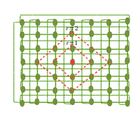
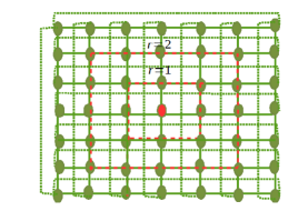
A two dimensional nearest neighbor torus can be defined in various ways as shown in the Fig. 3 and Fig. 4. To get the nearest neighbors in two dimensions, L1superscript๐ฟ1L^{1} norm, L2superscript๐ฟ2L^{2} norm, and Lโˆžsuperscript๐ฟL^{\infty} norm are used. For simple and convenient analysis [14], L1superscript๐ฟ1L^{1} norm and Lโˆžsuperscript๐ฟL^{\infty} norm are preferable, where L1superscript๐ฟ1L^{1} norm is used when there is an connection between nodes whose shortest path is within r๐‘Ÿr hops on the torus and Lโˆžsuperscript๐ฟL^{\infty} norm is used when vertical and horizontal distance are both within r๐‘Ÿr hops on the torus.

Refer to caption
Figure 3: L1superscript๐ฟ1L^{1} Nearest neighbor torus.
Refer to caption
Figure 4: Lโˆžsuperscript๐ฟL^{\infty} Nearest neighbor torus.

IV Convergence analysis for r๐‘Ÿr-nearest neighbor networks

After calculating the eigenvalue expressions, the steps for calculating the optimal consensus parameter hโ„Žh, optimal convergence parameter ฮณ๐›พ\gamma, and convergence time T๐‘‡T are as follows:
(1) Observe the second largest and smallest eigenvalues of W๐‘ŠW.
(2) Calculate hโ„Žh using ฮป2โ€‹(W)=โˆ’ฮปnโ€‹(W)subscript๐œ†2๐‘Šsubscript๐œ†๐‘›๐‘Š\lambda_{2}(W)=-\lambda_{n}(W), here ฮป2โ€‹(W)subscript๐œ†2๐‘Š\lambda_{2}(W) is a second largest eigenvalue of W๐‘ŠW and ฮปnโ€‹(W)subscript๐œ†๐‘›๐‘Š\lambda_{n}(W) is a smallest eigenvalue of W๐‘ŠW.
(3) Determine ฮณโ€‹(W)=mโ€‹aโ€‹xโ€‹{|1โˆ’hโ€‹ฮป2โ€‹(L)|,|1โˆ’hโ€‹ฮปnโ€‹(L)|}๐›พ๐‘Š๐‘š๐‘Ž๐‘ฅ1โ„Žsubscript๐œ†2๐ฟ1โ„Žsubscript๐œ†๐‘›๐ฟ\gamma(W)=max\left\{{\left|{1-h\lambda_{2}(L)}\right|,\left|{1-h\lambda_{n}(L)}\right|}\right\}.
(4) Finally, calculate the convergence time using T=1/(logโก(1/ฮณ))๐‘‡11๐›พT=1/\left({\log(1/\gamma)}\right) [21].

IV-A r๐‘Ÿr-nearest neighbor cycle

Tโ€‹hโ€‹eโ€‹oโ€‹rโ€‹eโ€‹m๐‘‡โ„Ž๐‘’๐‘œ๐‘Ÿ๐‘’๐‘šTheorem 666: Given an r๐‘Ÿr-nearest neighbor cycle Cnrsuperscriptsubscript๐ถ๐‘›๐‘ŸC_{n}^{r} and n๐‘›n is even, the optimal consensus parameter hโ„Žh is computed by

h=12โ€‹r+1โˆ’12โ€‹(sinโก(2โ€‹ฯ€โ€‹(r+0.5)n)sinโกฯ€n+cosโก(ฯ€โ€‹r)).โ„Ž12๐‘Ÿ1122๐œ‹๐‘Ÿ0.5๐‘›๐œ‹๐‘›๐œ‹๐‘Ÿh=\frac{1}{{2r+1-\frac{1}{2}\left({\frac{{\sin\left({\frac{{2\pi\left({r+0.5}\right)}}{n}}\right)}}{{\sin\frac{\pi}{n}}}+\cos(\pi r)}\right)}}. (36)

Pโ€‹rโ€‹oโ€‹oโ€‹f๐‘ƒ๐‘Ÿ๐‘œ๐‘œ๐‘“Proof : The proof is deferred to Appendix A.

Tโ€‹hโ€‹eโ€‹oโ€‹rโ€‹eโ€‹m๐‘‡โ„Ž๐‘’๐‘œ๐‘Ÿ๐‘’๐‘šTheorem 777: Given an r๐‘Ÿr-nearest neighbor cycle Cnrsuperscriptsubscript๐ถ๐‘›๐‘ŸC_{n}^{r} and n๐‘›n is odd, the optimal consensus parameter hโ„Žh is computed by

h=12โ€‹r+1โˆ’12โ€‹(sinโก((2โ€‹r+1)โ€‹ฯ€n)sinโกฯ€nโˆ’cosโก(ฯ€โ€‹(2โ€‹r+1)2โ€‹n)cosโกฯ€2โ€‹n).โ„Ž12๐‘Ÿ1122๐‘Ÿ1๐œ‹๐‘›๐œ‹๐‘›๐œ‹2๐‘Ÿ12๐‘›๐œ‹2๐‘›\leavevmode\resizebox{422.77661pt}{}{$h=\frac{1}{{2r+1-\frac{1}{2}\left({\frac{{\sin\left({\frac{{(2r+1)\pi}}{n}}\right)}}{{\sin\frac{\pi}{n}}}-\frac{{\cos\left({\frac{{\pi(2r+1)}}{{2n}}}\right)}}{{\cos\frac{\pi}{{2n}}}}}\right)}}$}. (37)

Pโ€‹rโ€‹oโ€‹oโ€‹f๐‘ƒ๐‘Ÿ๐‘œ๐‘œ๐‘“Proof : The proof is deferred to Appendix A.

Tโ€‹hโ€‹eโ€‹oโ€‹rโ€‹eโ€‹m๐‘‡โ„Ž๐‘’๐‘œ๐‘Ÿ๐‘’๐‘šTheorem 888: Given an r๐‘Ÿr-nearest neighbor cycle Cnrsuperscriptsubscript๐ถ๐‘›๐‘ŸC_{n}^{r} and n๐‘›n is even, the optimal convergence parameter ฮณ๐›พ\gamma is computed by

ฮณ=(sinโก((2โ€‹r+1)โ€‹ฯ€n)sinโกฯ€nโˆ’cosโก(ฯ€โ€‹r))4โ€‹r+2โˆ’(sinโก((2โ€‹r+1)โ€‹ฯ€n)sinโกฯ€n+cosโก(ฯ€โ€‹r)).๐›พ2๐‘Ÿ1๐œ‹๐‘›๐œ‹๐‘›๐œ‹๐‘Ÿ4๐‘Ÿ22๐‘Ÿ1๐œ‹๐‘›๐œ‹๐‘›๐œ‹๐‘Ÿ\gamma=\frac{{\left({\frac{{\sin\left({\frac{{(2r+1)\pi}}{n}}\right)}}{{\sin\frac{\pi}{n}}}-\cos(\pi r)}\right)}}{{4r+2-\left({\frac{{\sin\left({\frac{{(2r+1)\pi}}{n}}\right)}}{{\sin\frac{\pi}{n}}}+\cos(\pi r)}\right)}}. (38)

Pโ€‹rโ€‹oโ€‹oโ€‹f๐‘ƒ๐‘Ÿ๐‘œ๐‘œ๐‘“Proof : The proof is deferred to Appendix A.

Tโ€‹hโ€‹eโ€‹oโ€‹rโ€‹eโ€‹m๐‘‡โ„Ž๐‘’๐‘œ๐‘Ÿ๐‘’๐‘šTheorem 999: Given an r๐‘Ÿr-nearest neighbor cycle Cnrsuperscriptsubscript๐ถ๐‘›๐‘ŸC_{n}^{r} and n๐‘›n is odd, the optimal convergence parameter ฮณ๐›พ\gamma is

ฮณ=(sinโก((2โ€‹r+1)โ€‹ฯ€n)sinโกฯ€n+cosโก(ฯ€โ€‹(2โ€‹r+1)2โ€‹n)cosโกฯ€2โ€‹n)4โ€‹r+2โˆ’(sinโก((2โ€‹r+1)โ€‹ฯ€n)sinโกฯ€nโˆ’cosโก(ฯ€โ€‹(2โ€‹r+1)2โ€‹n)cosโกฯ€2โ€‹n).๐›พ2๐‘Ÿ1๐œ‹๐‘›๐œ‹๐‘›๐œ‹2๐‘Ÿ12๐‘›๐œ‹2๐‘›4๐‘Ÿ22๐‘Ÿ1๐œ‹๐‘›๐œ‹๐‘›๐œ‹2๐‘Ÿ12๐‘›๐œ‹2๐‘›\leavevmode\resizebox{422.77661pt}{}{$\gamma=\frac{{\left({\frac{{\sin\left({\frac{{(2r+1)\pi}}{n}}\right)}}{{\sin\frac{\pi}{n}}}+\frac{{\cos\left({\frac{{\pi(2r+1)}}{{2n}}}\right)}}{{\cos\frac{\pi}{{2n}}}}}\right)}}{{4r+2-\left({\frac{{\sin\left({\frac{{(2r+1)\pi}}{n}}\right)}}{{\sin\frac{\pi}{n}}}-\frac{{\cos\left({\frac{{\pi(2r+1)}}{{2n}}}\right)}}{{\cos\frac{\pi}{{2n}}}}}\right)}}$}. (39)

Pโ€‹rโ€‹oโ€‹oโ€‹f๐‘ƒ๐‘Ÿ๐‘œ๐‘œ๐‘“Proof : The proof is deferred to Appendix A.

IV-B r๐‘Ÿr-nearest neighbor torus

Tโ€‹hโ€‹eโ€‹oโ€‹rโ€‹eโ€‹m๐‘‡โ„Ž๐‘’๐‘œ๐‘Ÿ๐‘’๐‘šTheorem 101010: Given an r๐‘Ÿr-nearest neighbor torus Tk1,k2rsuperscriptsubscript๐‘‡subscript๐‘˜1subscript๐‘˜2๐‘ŸT_{k_{1},k_{2}}^{r} and k1,k2subscript๐‘˜1subscript๐‘˜2k_{1},k_{2} are even integers, the optimal consensus parameter is

h=11.5+3โ€‹rโˆ’12โ€‹(sinโก((2โ€‹r+1)โ€‹ฯ€k2)sinโกฯ€k2+2โ€‹cosโก(ฯ€โ€‹r)).โ„Ž11.53๐‘Ÿ122๐‘Ÿ1๐œ‹subscript๐‘˜2๐œ‹subscript๐‘˜22๐œ‹๐‘Ÿh=\frac{1}{{1.5+3r-\frac{1}{2}\left({\frac{{\sin\left({\frac{{(2r+1)\pi}}{{k_{2}}}}\right)}}{{\sin\frac{\pi}{{k_{2}}}}}+2\cos(\pi r)}\right)}}. (40)

Pโ€‹rโ€‹oโ€‹oโ€‹f๐‘ƒ๐‘Ÿ๐‘œ๐‘œ๐‘“Proof : The proof is deferred to Appendix B.

Tโ€‹hโ€‹eโ€‹oโ€‹rโ€‹eโ€‹m๐‘‡โ„Ž๐‘’๐‘œ๐‘Ÿ๐‘’๐‘šTheorem 111111: Given an r๐‘Ÿr-nearest neighbor torus Tk1,k2rsuperscriptsubscript๐‘‡subscript๐‘˜1subscript๐‘˜2๐‘ŸT_{k_{1},k_{2}}^{r} and k1,k2subscript๐‘˜1subscript๐‘˜2k_{1},k_{2} are odd integers, the optimal consensus parameter is expressed as

h=11.5+3โ€‹rโˆ’0.5โ€‹(sinโก((2โ€‹r+1)โ€‹ฯ€k2)sinโก(ฯ€k2)+sinโก(ฯ€โ€‹(2โ€‹r+1)โ€‹(k1โˆ’1)2โ€‹k1)sinโก(ฯ€โ€‹(k1โˆ’1)2โ€‹k1)+sinโก(ฯ€โ€‹(2โ€‹r+1)โ€‹(k2โˆ’1)2โ€‹k2)sinโก(ฯ€โ€‹(k2โˆ’1)2โ€‹k2)).โ„Ž11.53๐‘Ÿ0.52๐‘Ÿ1๐œ‹subscript๐‘˜2๐œ‹subscript๐‘˜2๐œ‹2๐‘Ÿ1subscript๐‘˜112subscript๐‘˜1๐œ‹subscript๐‘˜112subscript๐‘˜1๐œ‹2๐‘Ÿ1subscript๐‘˜212subscript๐‘˜2๐œ‹subscript๐‘˜212subscript๐‘˜2\leavevmode\resizebox{422.77661pt}{}{$h=\frac{1}{{1.5+3r-0.5\left({\frac{{\sin\left({\frac{{(2r+1)\pi}}{{k_{2}}}}\right)}}{{\sin\left({\frac{\pi}{{k_{2}}}}\right)}}+\frac{{\sin\left({\frac{{\pi(2r+1)(k_{1}-1)}}{{2k_{1}}}}\right)}}{{\sin\left({\frac{{\pi(k_{1}-1)}}{{2k_{1}}}}\right)}}+\frac{{\sin\left({\frac{{\pi(2r+1)(k_{2}-1)}}{{2k_{2}}}}\right)}}{{\sin\left({\frac{{\pi(k_{2}-1)}}{{2k_{2}}}}\right)}}}\right)}}$}. (41)

Pโ€‹rโ€‹oโ€‹oโ€‹f๐‘ƒ๐‘Ÿ๐‘œ๐‘œ๐‘“Proof : The proof is deferred to Appendix B.

Tโ€‹hโ€‹eโ€‹oโ€‹rโ€‹eโ€‹m๐‘‡โ„Ž๐‘’๐‘œ๐‘Ÿ๐‘’๐‘šTheorem 121212: Given an r๐‘Ÿr-nearest neighbor torus Tk1,k2rsuperscriptsubscript๐‘‡subscript๐‘˜1subscript๐‘˜2๐‘ŸT_{k_{1},k_{2}}^{r} and k1,k2subscript๐‘˜1subscript๐‘˜2k_{1},k_{2} are even integers, the optimal convergence parameter is

ฮณ=r+0.5+0.5โ€‹(sinโก((2โ€‹r+1)โ€‹ฯ€k2)sinโก(ฯ€k2)โˆ’2โ€‹cosโกฯ€โ€‹r)(1.5+3โ€‹r)โˆ’0.5โ€‹(sinโก((2โ€‹r+1)โ€‹ฯ€k2)sinโก(ฯ€k2)+2โ€‹cosโกฯ€โ€‹r).๐›พ๐‘Ÿ0.50.52๐‘Ÿ1๐œ‹subscript๐‘˜2๐œ‹subscript๐‘˜22๐œ‹๐‘Ÿ1.53๐‘Ÿ0.52๐‘Ÿ1๐œ‹subscript๐‘˜2๐œ‹subscript๐‘˜22๐œ‹๐‘Ÿ\gamma=\frac{{r+0.5+0.5\left({\frac{{\sin\left({\frac{{(2r+1)\pi}}{{k_{2}}}}\right)}}{{\sin\left({\frac{\pi}{{k_{2}}}}\right)}}-2\cos\pi r}\right)}}{{(1.5+3r)-0.5\left({\frac{{\sin\left({\frac{{(2r+1)\pi}}{{k_{2}}}}\right)}}{{\sin\left({\frac{\pi}{{k_{2}}}}\right)}}+2\cos\pi r}\right)}}. (42)

Pโ€‹rโ€‹oโ€‹oโ€‹f๐‘ƒ๐‘Ÿ๐‘œ๐‘œ๐‘“Proof : The proof is deferred to Appendix B.
Tโ€‹hโ€‹eโ€‹oโ€‹rโ€‹eโ€‹m๐‘‡โ„Ž๐‘’๐‘œ๐‘Ÿ๐‘’๐‘šTheorem 131313: Given an r๐‘Ÿr-nearest neighbor torus Tk1,k2rsuperscriptsubscript๐‘‡subscript๐‘˜1subscript๐‘˜2๐‘ŸT_{k_{1},k_{2}}^{r} and k1,k2subscript๐‘˜1subscript๐‘˜2k_{1},k_{2} are odd integers, the optimal convergence parameter is

ฮณ=r+0.5+0.5โ€‹(sinโก(ฯ€โ€‹(2โ€‹r+1)โ€‹(k1โˆ’1)2โ€‹k1)sinโก(ฯ€โ€‹(k1โˆ’1)2โ€‹k1)โˆ’sinโก((2โ€‹r+1)โ€‹ฯ€k2)sinโก(ฯ€k2)+sinโก(ฯ€โ€‹(2โ€‹r+1)โ€‹(k2โˆ’1)2โ€‹k2)sinโก(ฯ€โ€‹(k2โˆ’1)2โ€‹k2))(1.5+3โ€‹r)โˆ’0.5โ€‹(sinโก(ฯ€โ€‹(2โ€‹r+1)โ€‹(k1โˆ’1)2โ€‹k1)sinโก(ฯ€โ€‹(k1โˆ’1)2โ€‹k1)+sinโก((2โ€‹r+1)โ€‹ฯ€k2)sinโก(ฯ€k2)+sinโก(ฯ€โ€‹(2โ€‹r+1)โ€‹(k2โˆ’1)2โ€‹k2)sinโก(ฯ€โ€‹(k2โˆ’1)2โ€‹k2)).๐›พ๐‘Ÿ0.50.5๐œ‹2๐‘Ÿ1subscript๐‘˜112subscript๐‘˜1๐œ‹subscript๐‘˜112subscript๐‘˜12๐‘Ÿ1๐œ‹subscript๐‘˜2๐œ‹subscript๐‘˜2๐œ‹2๐‘Ÿ1subscript๐‘˜212subscript๐‘˜2๐œ‹subscript๐‘˜212subscript๐‘˜21.53๐‘Ÿ0.5๐œ‹2๐‘Ÿ1subscript๐‘˜112subscript๐‘˜1๐œ‹subscript๐‘˜112subscript๐‘˜12๐‘Ÿ1๐œ‹subscript๐‘˜2๐œ‹subscript๐‘˜2๐œ‹2๐‘Ÿ1subscript๐‘˜212subscript๐‘˜2๐œ‹subscript๐‘˜212subscript๐‘˜2\leavevmode\resizebox{422.77661pt}{}{$\gamma=\frac{{r+0.5+0.5\left({\frac{{\sin\left({\frac{{\pi(2r+1)(k_{1}-1)}}{{2k_{1}}}}\right)}}{{\sin\left({\frac{{\pi(k_{1}-1)}}{{2k_{1}}}}\right)}}-\frac{{\sin\left({\frac{{(2r+1)\pi}}{{k_{2}}}}\right)}}{{\sin\left({\frac{\pi}{{k_{2}}}}\right)}}+\frac{{\sin\left({\frac{{\pi(2r+1)(k_{2}-1)}}{{2k_{2}}}}\right)}}{{\sin\left({\frac{{\pi(k_{2}-1)}}{{2k_{2}}}}\right)}}}\right)}}{{(1.5+3r)-0.5\left({\frac{{\sin\left({\frac{{\pi(2r+1)(k_{1}-1)}}{{2k_{1}}}}\right)}}{{\sin\left({\frac{{\pi(k_{1}-1)}}{{2k_{1}}}}\right)}}+\frac{{\sin\left({\frac{{(2r+1)\pi}}{{k_{2}}}}\right)}}{{\sin\left({\frac{\pi}{{k_{2}}}}\right)}}+\frac{{\sin\left({\frac{{\pi(2r+1)(k_{2}-1)}}{{2k_{2}}}}\right)}}{{\sin\left({\frac{{\pi(k_{2}-1)}}{{2k_{2}}}}\right)}}}\right)}}$}. (43)

Pโ€‹rโ€‹oโ€‹oโ€‹f๐‘ƒ๐‘Ÿ๐‘œ๐‘œ๐‘“Proof : The proof is deferred to Appendix B.
Most of the WSN applications, such as space monitoring, cave monitoring and studying underwater eco system operates in multiple dimensions. So without loss of generality, we have also derived the expressions for hโ„Žh and ฮณ๐›พ\gamma of m๐‘šm-dimensional torus networks.

IV-C m๐‘šm-dimensional torus

Tโ€‹hโ€‹eโ€‹oโ€‹rโ€‹eโ€‹m๐‘‡โ„Ž๐‘’๐‘œ๐‘Ÿ๐‘’๐‘šTheorem 141414: Given a m๐‘šm-dimensional r๐‘Ÿr-nearest neighbor torus and k1,k2,k3โ€‹โ€ฆโ€‹kmsubscript๐‘˜1subscript๐‘˜2subscript๐‘˜3โ€ฆsubscript๐‘˜๐‘šk_{1},k_{2},k_{3}...k_{m} are even integers, the optimal consensus parameter is computed by

h=1(m+1)โ€‹(r+0.5)โˆ’0.5โ€‹sinโก((2โ€‹r+1)โ€‹ฯ€k1)sinโก(ฯ€k1)โˆ’mโ€‹cosโกฯ€โ€‹r2.โ„Ž1๐‘š1๐‘Ÿ0.50.52๐‘Ÿ1๐œ‹subscript๐‘˜1๐œ‹subscript๐‘˜1๐‘š๐œ‹๐‘Ÿ2h=\frac{1}{{(m+1)(r+0.5)-\frac{{0.5\sin\left({\frac{{(2r+1)\pi}}{{k_{1}}}}\right)}}{{\sin\left({\frac{\pi}{{k_{1}}}}\right)}}-\frac{{m\cos\pi r}}{2}}}. (44)

Pโ€‹rโ€‹oโ€‹oโ€‹f๐‘ƒ๐‘Ÿ๐‘œ๐‘œ๐‘“Proof : The proof is deferred to Appendix C.

Tโ€‹hโ€‹eโ€‹oโ€‹rโ€‹eโ€‹m๐‘‡โ„Ž๐‘’๐‘œ๐‘Ÿ๐‘’๐‘šTheorem 151515: Given a m๐‘šm-dimensional r๐‘Ÿr-nearest neighbor torus and k1,k2,k3โ€‹โ€ฆโ€‹kmsubscript๐‘˜1subscript๐‘˜2subscript๐‘˜3โ€ฆsubscript๐‘˜๐‘šk_{1},k_{2},k_{3}...k_{m} are odd integers, the optimal consensus parameter is computed by

h=1(m+1)โ€‹(r+0.5)โˆ’0.5โ€‹sinโก((2โ€‹r+1)โ€‹ฯ€k1)sinโก(ฯ€k1)โˆ’โˆ‘l=1m0.5โ€‹sinโก((2โ€‹r+1)โ€‹ฯ€โ€‹(klโˆ’1)2โ€‹kl)sinโก(ฯ€โ€‹(klโˆ’1)2โ€‹kl).โ„Ž1๐‘š1๐‘Ÿ0.50.52๐‘Ÿ1๐œ‹subscript๐‘˜1๐œ‹subscript๐‘˜1superscriptsubscript๐‘™1๐‘š0.52๐‘Ÿ1๐œ‹subscript๐‘˜๐‘™12subscript๐‘˜๐‘™๐œ‹subscript๐‘˜๐‘™12subscript๐‘˜๐‘™\leavevmode\resizebox{422.77661pt}{}{$h=\frac{1}{{(m+1)(r+0.5)-\frac{{0.5\sin\left({\frac{{(2r+1)\pi}}{{k_{1}}}}\right)}}{{\sin\left({\frac{\pi}{{k_{1}}}}\right)}}-\sum\limits_{l=1}^{m}{\frac{{0.5\sin\left({\frac{{(2r+1)\pi(k_{l}-1)}}{{2k_{l}}}}\right)}}{{\sin\left({\frac{{\pi(k_{l}-1)}}{{2k_{l}}}}\right)}}}}}$}. (45)

Pโ€‹rโ€‹oโ€‹oโ€‹f๐‘ƒ๐‘Ÿ๐‘œ๐‘œ๐‘“Proof : The proof is deferred to Appendix C.
Tโ€‹hโ€‹eโ€‹oโ€‹rโ€‹eโ€‹m๐‘‡โ„Ž๐‘’๐‘œ๐‘Ÿ๐‘’๐‘šTheorem 161616: Given a m๐‘šm-dimensional r๐‘Ÿr-nearest neighbor torus and k1,k2,k3โ€‹โ€ฆโ€‹kmsubscript๐‘˜1subscript๐‘˜2subscript๐‘˜3โ€ฆsubscript๐‘˜๐‘šk_{1},k_{2},k_{3}...k_{m} are even integers, the optimal convergence parameter is computed by

ฮณ=(mโˆ’1)โ€‹(r+0.5)+0.5โ€‹sinโก((2โ€‹r+1)โ€‹ฯ€k1)sinโก(ฯ€k1)โˆ’m2โ€‹cosโก(ฯ€โ€‹r)(m+1)โ€‹(r+0.5)โˆ’0.5โ€‹sinโก((2โ€‹r+1)โ€‹ฯ€k1)sinโก(ฯ€k1)โˆ’m2โ€‹cosโก(ฯ€โ€‹r).๐›พ๐‘š1๐‘Ÿ0.50.52๐‘Ÿ1๐œ‹subscript๐‘˜1๐œ‹subscript๐‘˜1๐‘š2๐œ‹๐‘Ÿ๐‘š1๐‘Ÿ0.50.52๐‘Ÿ1๐œ‹subscript๐‘˜1๐œ‹subscript๐‘˜1๐‘š2๐œ‹๐‘Ÿ\leavevmode\resizebox{422.77661pt}{}{$\gamma=\frac{{(m-1)(r+0.5)+\frac{{0.5\sin\left({\frac{{(2r+1)\pi}}{{k_{1}}}}\right)}}{{\sin\left({\frac{\pi}{{k_{1}}}}\right)}}-\frac{m}{2}\cos(\pi r)}}{{(m+1)(r+0.5)-\frac{{0.5\sin\left({\frac{{(2r+1)\pi}}{{k_{1}}}}\right)}}{{\sin\left({\frac{\pi}{{k_{1}}}}\right)}}-\frac{m}{2}\cos(\pi r)}}$}. (46)

Pโ€‹rโ€‹oโ€‹oโ€‹f๐‘ƒ๐‘Ÿ๐‘œ๐‘œ๐‘“Proof : The proof is deferred to Appendix C.
Tโ€‹hโ€‹eโ€‹oโ€‹rโ€‹eโ€‹mโ€‹17๐‘‡โ„Ž๐‘’๐‘œ๐‘Ÿ๐‘’๐‘š17Theorem17: Given a m๐‘šm-dimensional r๐‘Ÿr-nearest neighbor torus and k1,k2,k3โ€‹โ€ฆโ€‹kmsubscript๐‘˜1subscript๐‘˜2subscript๐‘˜3โ€ฆsubscript๐‘˜๐‘šk_{1},k_{2},k_{3}...k_{m} are odd integers, the optimal convergence parameter is computed by

ฮณ=(mโˆ’1)โ€‹(r+0.5)+12โ€‹(sinโก(r+0.5)โ€‹2โ€‹ฯ€k1sinโกฯ€k1โˆ’โˆ‘l=1msinโก(r+0.5)โ€‹ฯ€โ€‹(klโˆ’1)klsinโกฯ€โ€‹(klโˆ’1)2โ€‹kl)(m+1)โ€‹(r+0.5)โˆ’12โ€‹(sinโก(r+0.5)โ€‹2โ€‹ฯ€k1sinโกฯ€k1+โˆ‘l=1msinโก(r+0.5)โ€‹ฯ€โ€‹(klโˆ’1)klsinโกฯ€โ€‹(klโˆ’1)2โ€‹kl).๐›พ๐‘š1๐‘Ÿ0.512๐‘Ÿ0.52๐œ‹subscript๐‘˜1๐œ‹subscript๐‘˜1superscriptsubscript๐‘™1๐‘š๐‘Ÿ0.5๐œ‹subscript๐‘˜๐‘™1subscript๐‘˜๐‘™๐œ‹subscript๐‘˜๐‘™12subscript๐‘˜๐‘™๐‘š1๐‘Ÿ0.512๐‘Ÿ0.52๐œ‹subscript๐‘˜1๐œ‹subscript๐‘˜1superscriptsubscript๐‘™1๐‘š๐‘Ÿ0.5๐œ‹subscript๐‘˜๐‘™1subscript๐‘˜๐‘™๐œ‹subscript๐‘˜๐‘™12subscript๐‘˜๐‘™\leavevmode\resizebox{422.77661pt}{}{$\gamma=\frac{{(m-1)(r+0.5)+\frac{1}{2}\left({\frac{{\sin\frac{{(r+0.5)2\pi}}{{k_{1}}}}}{{\sin\frac{\pi}{{k_{1}}}}}-\sum\limits_{l=1}^{m}{\frac{{\sin\frac{{(r+0.5)\pi(k_{l}-1)}}{{k_{l}}}}}{{\sin\frac{{\pi(k_{l}-1)}}{{2k_{l}}}}}}}\right)}}{{(m+1)(r+0.5)-\frac{1}{2}\left({\frac{{\sin\frac{{(r+0.5)2\pi}}{{k_{1}}}}}{{\sin\frac{\pi}{{k_{1}}}}}+\sum\limits_{l=1}^{m}{\frac{{\sin\frac{{(r+0.5)\pi(k_{l}-1)}}{{k_{l}}}}}{{\sin\frac{{\pi(k_{l}-1)}}{{2k_{l}}}}}}}\right)}}$}. (47)

Pโ€‹rโ€‹oโ€‹oโ€‹f๐‘ƒ๐‘Ÿ๐‘œ๐‘œ๐‘“Proof : The proof is deferred to Appendix C.

V Numerical results and Discussion

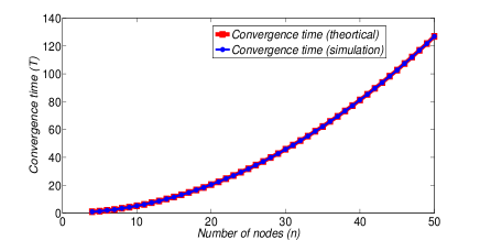
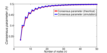
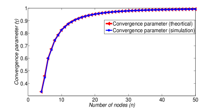
In this section, we present numerical results to examine the effect of n๐‘›n, m๐‘šm, and r๐‘Ÿr on the hโ„Žh, ฮณ๐›พ\gamma, and T๐‘‡T. Plots of the hโ„Žh versus n๐‘›n for 1-nearest neighbor cycle are shown in Fig. 5. We have observed that hโ„Žh increases with n๐‘›n for small scale systems,and from n=40๐‘›40n=40, optimal weight approaches approximately 0.50.50.5. Plots of ฮณ๐›พ\gamma versus n๐‘›n and T๐‘‡T versus n๐‘›n for r=1๐‘Ÿ1r=1, are shown in Fig. 6 and Fig. 7 respectively. Convergence time T๐‘‡T values have been calculated using (38) and (39), for Fig. 7. As n๐‘›n increases, ฮณ๐›พ\gamma increases and approaches unity for large scale systems as shown in Fig. 6. From Fig. 7, we can observe that T๐‘‡T increases exponentially with n๐‘›n.

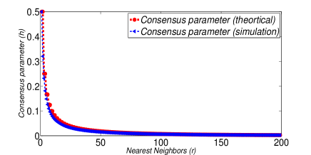
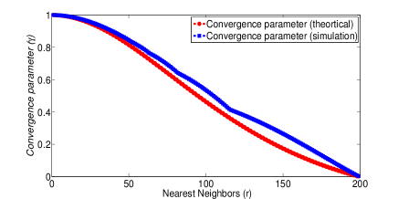
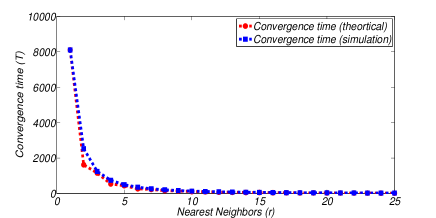
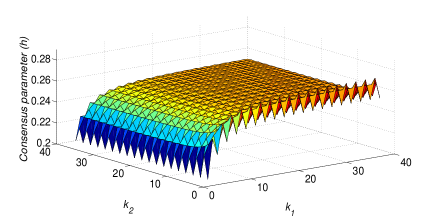
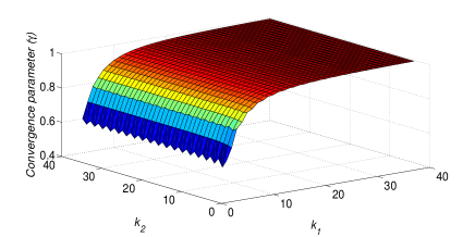
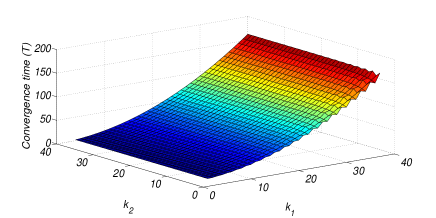
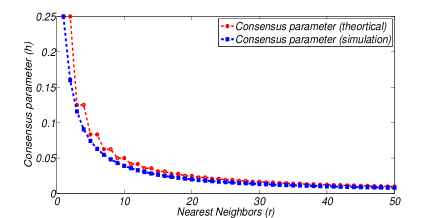
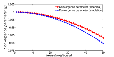
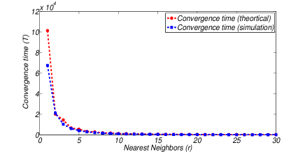
Figs. 8, 9, and 10 show plots of the hโ„Žh, ฮณ๐›พ\gamma, and T๐‘‡T versus r๐‘Ÿr for n=400๐‘›400n=400 respectively. From Fig. 8, We find that hโ„Žh decreases exponentially with r๐‘Ÿr and ฮณ๐›พ\gamma decreases linearly with r๐‘Ÿr. From Fig. 10, we can see that T๐‘‡T decreases exponentially with r๐‘Ÿr, since the links or edges between every node increases with r๐‘Ÿr directly influence the consensus process which in turn decreases the convergence time. Note that, from r=10๐‘Ÿ10r=10, T๐‘‡T values are almost constant irrespective of increase in r๐‘Ÿr values. Figs. 11, 12, and 13 show plots of the hโ„Žh, ฮณ๐›พ\gamma, and T๐‘‡T versus k1subscript๐‘˜1k_{1} and k2subscript๐‘˜2k_{2} for respectively. We have used the (40), (41), (42), and (43) to compute the hโ„Žh, ฮณ๐›พ\gamma, and T๐‘‡T values for r=1๐‘Ÿ1r=1. It is observed that optimal weight hโ„Žh increases and approaches 0.250.250.25 in two dimensional WSNs for r=1๐‘Ÿ1r=1. As shown in Figs. 12 and 13, ฮณ๐›พ\gamma increases with k1subscript๐‘˜1k_{1} and k2subscript๐‘˜2k_{2} and approaches unity and T๐‘‡T increases compared to Fig.7, because of the increase in total number of nodes in torus network.

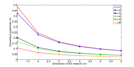
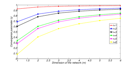
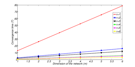
Figs. 14, 15, and 16 show plots of the hโ„Žh, ฮณ๐›พ\gamma, and T๐‘‡T versus r๐‘Ÿr respectively. For ease of analysis, we have assumed that k1=1000subscript๐‘˜11000k_{1}=1000 and k2=1000subscript๐‘˜21000k_{2}=1000, and observe that hโ„Žh, ฮณ๐›พ\gamma, and T๐‘‡T decreases with r๐‘Ÿr. Plots of hโ„Žh, ฮณ๐›พ\gamma, and T๐‘‡T versus m๐‘šm with varying number of r๐‘Ÿr values are shown in Figs. 17, 18, and 19 respectively. In this case, we have assumed that k1subscript๐‘˜1k_{1} = 16, k2subscript๐‘˜2k_{2} = 18, k3subscript๐‘˜3k_{3} = 20, k4subscript๐‘˜4k_{4} = 22, k5subscript๐‘˜5k_{5} = 24, and k6subscript๐‘˜6k_{6} = 26. As shown in the Fig. 17, optimal weight hโ„Žh decreases with m๐‘šm for various r๐‘Ÿr values and a drastic decrease can be observed from r=2๐‘Ÿ2r=2 to r=3๐‘Ÿ3r=3 and r=4๐‘Ÿ4r=4 to r=5๐‘Ÿ5r=5. As shown in the Fig. 18, ฮณ๐›พ\gamma values approaches different values which are less than unity depends on m๐‘šm and r๐‘Ÿr values. Fig. 19 shows that convergence time T๐‘‡T increases linearly with m๐‘šm, but the increase in r๐‘Ÿr results in substantial decay of T๐‘‡T values.

V-A Convergence time-overhead Optimization

Using the expressions derived in Tโ€‹hโ€‹eโ€‹oโ€‹rโ€‹eโ€‹m๐‘‡โ„Ž๐‘’๐‘œ๐‘Ÿ๐‘’๐‘šTheorem 888, Tโ€‹hโ€‹eโ€‹oโ€‹rโ€‹eโ€‹m๐‘‡โ„Ž๐‘’๐‘œ๐‘Ÿ๐‘’๐‘šTheorem 999, Tโ€‹hโ€‹eโ€‹oโ€‹rโ€‹eโ€‹m๐‘‡โ„Ž๐‘’๐‘œ๐‘Ÿ๐‘’๐‘šTheorem 121212, Tโ€‹hโ€‹eโ€‹oโ€‹rโ€‹eโ€‹m๐‘‡โ„Ž๐‘’๐‘œ๐‘Ÿ๐‘’๐‘šTheorem 131313, Tโ€‹hโ€‹eโ€‹oโ€‹rโ€‹eโ€‹m๐‘‡โ„Ž๐‘’๐‘œ๐‘Ÿ๐‘’๐‘šTheorem 161616, and Tโ€‹hโ€‹eโ€‹oโ€‹rโ€‹eโ€‹m๐‘‡โ„Ž๐‘’๐‘œ๐‘Ÿ๐‘’๐‘šTheorem 171717, we can estimate the trade-off between convergence time and overhead. From the Figs. 10, 16, and 19, we can observe that nearest neighbors or node transmission radius is exponentially reducing the convergence time, which is a primary objective of consensus algorithm. But the nodeโ€™s power consumption [17] is

P=(rn)ฮฑ๐‘ƒsuperscript๐‘Ÿ๐‘›๐›ผP=\left(\frac{r}{\sqrt{n}}\right)^{\alpha} (48)

where ฮฑ๐›ผ\alpha is a path-loss exponent. So it has to be noted that while applying consensus algorithms on WSNs, it is also necessary to take care about the nodeโ€™s power consumption since sensor nodes consist of limited power resources. We propose an optimization framework, to minimize the convergence time T๐‘‡T subject to total power consumption constraint and minimizing the power consumption subject to maximum convergence time.

minimize T๐‘‡\displaystyle T
subject to rโ‰คrmโ€‹aโ€‹x,Pโ‰คPmโ€‹aโ€‹xformulae-sequence๐‘Ÿsubscript๐‘Ÿ๐‘š๐‘Ž๐‘ฅ๐‘ƒsubscript๐‘ƒ๐‘š๐‘Ž๐‘ฅ\displaystyle r\leq r_{max},\;P\leq P_{max}
minimize P๐‘ƒ\displaystyle P
subject to Tโ‰คTmโ€‹aโ€‹x,rโ‰คrmโ€‹aโ€‹xformulae-sequence๐‘‡subscript๐‘‡๐‘š๐‘Ž๐‘ฅ๐‘Ÿsubscript๐‘Ÿ๐‘š๐‘Ž๐‘ฅ\displaystyle T\leq T_{max},\;r\leq r_{max}

where rmโ€‹aโ€‹xsubscript๐‘Ÿ๐‘š๐‘Ž๐‘ฅr_{max}, Tmโ€‹aโ€‹xsubscript๐‘‡๐‘š๐‘Ž๐‘ฅT_{max}, and Pmโ€‹aโ€‹xsubscript๐‘ƒ๐‘š๐‘Ž๐‘ฅP_{max} are certain threshold values defined based on WSN resource requirements. The solutions can be obtained by calculating the respective Lagrangian values.
Refer to caption
Figure 5: Comparison of theoretical and simulation results for consensus parameter hโ„Žh of 111-nearest neighbor cycle.
Refer to caption
Figure 6: Comparison of theoretical and simulation results for convergence parameter ฮณ๐›พ\gamma of 111-nearest neighbor cycle.
Refer to caption
Figure 7: Comparison of theoretical and simulation results for convergence time T๐‘‡T of 111-nearest neighbor cycle.
Refer to caption
Figure 8: Comparison of theoretical and simulation results for consensus parameter hโ„Žh of r๐‘Ÿr-nearest neighbor cycle for n=400.
Refer to caption
Figure 9: Comparison of theoretical and simulation results for convergence parameter ฮณ๐›พ\gamma of r๐‘Ÿr-nearest neighbor cycle for n=400.
Refer to caption
Figure 10: Comparison of theoretical and simulation results for convergence time T๐‘‡T of r๐‘Ÿr-nearest neighbor cycle for n=400.
Refer to caption
Figure 11: Consensus parameter hโ„Žh versus k1subscript๐‘˜1k_{1}, k2subscript๐‘˜2k_{2} of r๐‘Ÿr-nearest neighbor torus for r=1๐‘Ÿ1r=1.
Refer to caption
Figure 12: Convergence parameter ฮณ๐›พ\gamma versus k1subscript๐‘˜1k_{1}, k2subscript๐‘˜2k_{2} of r๐‘Ÿr-nearest neighbor torus for r=1๐‘Ÿ1r=1.
Refer to caption
Figure 13: Convergence time T๐‘‡T versus k1subscript๐‘˜1k_{1}, k2subscript๐‘˜2k_{2} of r๐‘Ÿr-nearest neighbor torus for r=1๐‘Ÿ1r=1.
Refer to caption
Figure 14: Comparison of theoretical and simulation results for consensus parameter hโ„Žh of r๐‘Ÿr-nearest neighbor torus for k1=k2=1000subscript๐‘˜1subscript๐‘˜21000k_{1}=k_{2}=1000.
Refer to caption
Figure 15: Comparison of theoretical and simulation results for convergence parameter ฮณ๐›พ\gamma of r๐‘Ÿr-nearest neighbor torus for k1=k2=1000subscript๐‘˜1subscript๐‘˜21000k_{1}=k_{2}=1000.
Refer to caption
Figure 16: Comparison of theoretical and simulation results for convergence time T๐‘‡T of r๐‘Ÿr-nearest neighbor torus for k1=k2=1000subscript๐‘˜1subscript๐‘˜21000k_{1}=k_{2}=1000.
Refer to caption
Figure 17: Consensus parameter hโ„Žh versus network dimension m๐‘šm of m๐‘šm-dimensional torus with varying number of nearest neighbors r๐‘Ÿr for k1subscript๐‘˜1k_{1} = 16, k2subscript๐‘˜2k_{2} = 18, k3subscript๐‘˜3k_{3} = 20, k4subscript๐‘˜4k_{4} = 22, k5subscript๐‘˜5k_{5} = 24, and k6subscript๐‘˜6k_{6} = 26.
Refer to caption
Figure 18: Convergence parameter ฮณ๐›พ\gamma versus network dimension m๐‘šm of m๐‘šm-dimensional torus with varying number of nearest neighbors r๐‘Ÿr for k1subscript๐‘˜1k_{1} = 16, k2subscript๐‘˜2k_{2} = 18, k3subscript๐‘˜3k_{3} = 20, k4subscript๐‘˜4k_{4} = 22, k5subscript๐‘˜5k_{5} = 24, and k6subscript๐‘˜6k_{6} = 26.
Refer to caption
Figure 19: Convergence time T๐‘‡T versus network dimension m๐‘šm of m๐‘šm-dimensional torus with varying number of nearest neighbors r๐‘Ÿr for k1subscript๐‘˜1k_{1} = 16, k2subscript๐‘˜2k_{2} = 18, k3subscript๐‘˜3k_{3} = 20, k4subscript๐‘˜4k_{4} = 22, k5subscript๐‘˜5k_{5} = 24, and k6subscript๐‘˜6k_{6} = 26.

VI Conclusions

In this paper, we have derived the analytical expressions for optimal consensus parameter, optimal convergence parameter to estimate the convergence time of m๐‘šm-dimensional WSNs. We have investigated that nodes in multidimensional WSNs require more nearest neighbors or large transmission radius without effecting the power consumption. We have also proposed a optimization framework to design and control the performance of consensus algorithm on WSNs. Furthermore, the analytical expressions derived in this paper are extremely useful to exactly estimate the convergence time for large WSNs with less computational complexity.

Appendix A r๐‘Ÿr-nearest neighbor cycle

Proofs of Tโ€‹hโ€‹eโ€‹oโ€‹rโ€‹eโ€‹m๐‘‡โ„Ž๐‘’๐‘œ๐‘Ÿ๐‘’๐‘šTheorem 666, Tโ€‹hโ€‹eโ€‹oโ€‹rโ€‹eโ€‹m๐‘‡โ„Ž๐‘’๐‘œ๐‘Ÿ๐‘’๐‘šTheorem 777, Tโ€‹hโ€‹eโ€‹oโ€‹rโ€‹eโ€‹m๐‘‡โ„Ž๐‘’๐‘œ๐‘Ÿ๐‘’๐‘šTheorem 888, and Tโ€‹hโ€‹eโ€‹oโ€‹rโ€‹eโ€‹m๐‘‡โ„Ž๐‘’๐‘œ๐‘Ÿ๐‘’๐‘šTheorem 999 are given below.
From Tโ€‹hโ€‹eโ€‹oโ€‹rโ€‹eโ€‹m๐‘‡โ„Ž๐‘’๐‘œ๐‘Ÿ๐‘’๐‘šTheorem 222, eigenvalue expressions of weight matrix W๐‘ŠW can be written as

ฮป0โ€‹(W)=(1โˆ’2โ€‹rโ€‹h)+2โ€‹h,subscript๐œ†0๐‘Š12๐‘Ÿโ„Ž2โ„Ž\lambda_{0}(W)=\left({1-2rh}\right)+2h, (49)
ฮป1โ€‹(W)=(1โˆ’2โ€‹rโ€‹h)+2โ€‹hโ€‹โˆ‘j=1rcosโก(2โ€‹ฯ€โ€‹jn),subscript๐œ†1๐‘Š12๐‘Ÿโ„Ž2โ„Žsuperscriptsubscript๐‘—1๐‘Ÿ2๐œ‹๐‘—๐‘›\lambda_{1}(W)=\left({1-2rh}\right)+2h\sum\limits_{j=1}^{r}{\cos\left({\frac{{2\pi j}}{n}}\right)}, (50)
ฮปn2โ€‹(W)=(1โˆ’2โ€‹rโ€‹h)+2โ€‹hโ€‹โˆ‘j=1rcosโก(ฯ€โ€‹j),subscript๐œ†๐‘›2๐‘Š12๐‘Ÿโ„Ž2โ„Žsuperscriptsubscript๐‘—1๐‘Ÿ๐œ‹๐‘—\lambda_{\frac{n}{2}}(W)=\left({1-2rh}\right)+2h\sum\limits_{j=1}^{r}{\cos\left({\pi j}\right)}, (51)
ฮป(nโˆ’1)2โ€‹(W)=(1โˆ’2โ€‹hโ€‹r)+2โ€‹hโ€‹โˆ‘i=1rcosโก(ฯ€โ€‹iโ€‹(nโˆ’1)n),subscript๐œ†๐‘›12๐‘Š12โ„Ž๐‘Ÿ2โ„Žsuperscriptsubscript๐‘–1๐‘Ÿ๐œ‹๐‘–๐‘›1๐‘›\lambda_{\frac{{(n-1)}}{2}}(W)=(1-2hr)+2h\sum\limits_{i=1}^{r}{\cos\left({\frac{{\pi i(n-1)}}{n}}\right)}, (52)

Note that ฮป1โ€‹(W)subscript๐œ†1๐‘Š\lambda_{1}(W) is a second largest eigenvalue and ฮปn2โ€‹(W)subscript๐œ†๐‘›2๐‘Š\lambda_{\frac{n}{2}}(W) is a smallest eigenvalue of W๐‘ŠW, where n๐‘›n is even integer. And ฮณ๐›พ\gamma is minimum, when

|ฮป1โ€‹(W)|=|ฮปn2โ€‹(W)|.subscript๐œ†1๐‘Šsubscript๐œ†๐‘›2๐‘Š\left|{\lambda_{1}(W)}\right|=\left|{\lambda_{\frac{n}{2}}(W)}\right|. (53)

Substitution of (50) and (51) in (53), results in

h=12โ€‹r+0.5โˆ’โˆ‘j=1rcosโก(2โ€‹ฯ€โ€‹jn)โˆ’โˆ‘j=1rcosโก(ฯ€โ€‹j).โ„Ž12๐‘Ÿ0.5superscriptsubscript๐‘—1๐‘Ÿ2๐œ‹๐‘—๐‘›superscriptsubscript๐‘—1๐‘Ÿ๐œ‹๐‘—h=\frac{1}{{2r+0.5-\sum\limits_{j=1}^{r}{\cos\left({\frac{{2\pi j}}{n}}\right)}-\sum\limits_{j=1}^{r}{\cos\left({\pi j}\right)}}}. (54)

Nโ€‹oโ€‹tโ€‹e๐‘๐‘œ๐‘ก๐‘’Note 1: Dirichlet kernel is expressed as

1+2โ€‹โˆ‘j=1rcosโก(jโ€‹x)=sinโก(r+12)โ€‹xsinโกx2.12superscriptsubscript๐‘—1๐‘Ÿ๐‘—๐‘ฅ๐‘Ÿ12๐‘ฅ๐‘ฅ21+2\sum\limits_{j=1}^{r}{\cos\left({jx}\right)}=\frac{{\sin\left({r+\frac{1}{2}}\right)x}}{{\sin\frac{x}{2}}}. (55)

Using (55), hโ„Žh can be rewritten as (36). Finally, substitution of (36) in (50) proves Tโ€‹hโ€‹eโ€‹oโ€‹rโ€‹eโ€‹m๐‘‡โ„Ž๐‘’๐‘œ๐‘Ÿ๐‘’๐‘šTheorem 888.
Since ฮปnโˆ’12โ€‹(W)subscript๐œ†๐‘›12๐‘Š\lambda_{\frac{n-1}{2}}(W) is a smallest eigenvalue, where n๐‘›n is odd integer, and ฮณ๐›พ\gamma is minimum, when

|ฮป1โ€‹(W)|=|ฮป(nโˆ’1)2โ€‹(W)|.subscript๐œ†1๐‘Šsubscript๐œ†๐‘›12๐‘Š\left|{\lambda_{1}(W)}\right|=\left|{\lambda_{\frac{{(n-1)}}{2}}(W)}\right|. (56)

Substitution of (50) and (52) in (56) results in

h=12โ€‹rโˆ’โˆ‘j=1rcosโก(2โ€‹ฯ€โ€‹jn)โˆ’โˆ‘j=1rcosโก(ฯ€โ€‹jโ€‹(nโˆ’2)n),โ„Ž12๐‘Ÿsuperscriptsubscript๐‘—1๐‘Ÿ2๐œ‹๐‘—๐‘›superscriptsubscript๐‘—1๐‘Ÿ๐œ‹๐‘—๐‘›2๐‘›h=\frac{1}{{2r-\sum\limits_{j=1}^{r}{\cos\left({\frac{{2\pi j}}{n}}\right)}-\sum\limits_{j=1}^{r}{\cos\left({\frac{{\pi j\left({n-2}\right)}}{n}}\right)}}}, (57)

So from (55), hโ„Žh can be further simplified as (37). Finally, substitution of (37) in (50), proves Tโ€‹hโ€‹eโ€‹oโ€‹rโ€‹eโ€‹m๐‘‡โ„Ž๐‘’๐‘œ๐‘Ÿ๐‘’๐‘šTheorem 999.

Appendix B r๐‘Ÿr-nearest neighbor two dimensional torus

Proofs of Tโ€‹hโ€‹eโ€‹oโ€‹rโ€‹eโ€‹m๐‘‡โ„Ž๐‘’๐‘œ๐‘Ÿ๐‘’๐‘šTheorem 101010, Tโ€‹hโ€‹eโ€‹oโ€‹rโ€‹eโ€‹m๐‘‡โ„Ž๐‘’๐‘œ๐‘Ÿ๐‘’๐‘šTheorem 111111, Tโ€‹hโ€‹eโ€‹oโ€‹rโ€‹eโ€‹m๐‘‡โ„Ž๐‘’๐‘œ๐‘Ÿ๐‘’๐‘šTheorem 121212, and Tโ€‹hโ€‹eโ€‹oโ€‹rโ€‹eโ€‹m๐‘‡โ„Ž๐‘’๐‘œ๐‘Ÿ๐‘’๐‘šTheorem 131313 are given below.
From Tโ€‹hโ€‹eโ€‹oโ€‹rโ€‹eโ€‹m๐‘‡โ„Ž๐‘’๐‘œ๐‘Ÿ๐‘’๐‘šTheorem 444, eigenvalue expressions of W๐‘ŠW can be written as

ฮป0,1โ€‹(W)=(1โˆ’2โ€‹hโ€‹r)+2โ€‹hโ€‹โˆ‘j=1rcosโก(2โ€‹ฯ€โ€‹jk2),subscript๐œ†01๐‘Š12โ„Ž๐‘Ÿ2โ„Žsuperscriptsubscript๐‘—1๐‘Ÿ2๐œ‹๐‘—subscript๐‘˜2\lambda_{0,1}(W)=(1-2hr)+2h\sum\limits_{j=1}^{r}{\cos\left({\frac{{2\pi j}}{{k_{2}}}}\right)}, (58)
ฮปk12,k22โ€‹(W)=(1โˆ’4โ€‹hโ€‹r)+4โ€‹hโ€‹โˆ‘j=1rcosโก(ฯ€โ€‹j),subscript๐œ†subscript๐‘˜12subscript๐‘˜22๐‘Š14โ„Ž๐‘Ÿ4โ„Žsuperscriptsubscript๐‘—1๐‘Ÿ๐œ‹๐‘—\lambda_{\frac{k_{1}}{2},\frac{k_{2}}{2}}(W)=(1-4hr)+4h\sum\limits_{j=1}^{r}{\cos\left({\pi j}\right)}, (59)
ฮป(k1โˆ’1)2,(k2โˆ’1)2โ€‹(W)=(1โˆ’4โ€‹hโ€‹r)+2โ€‹hโ€‹โˆ‘j=1rcosโก(ฯ€โ€‹jโ€‹(k1โˆ’1)k1)+2โ€‹hโ€‹โˆ‘j=1rcosโก(ฯ€โ€‹jโ€‹(k2โˆ’1)k2).subscript๐œ†subscript๐‘˜112subscript๐‘˜212๐‘Š14โ„Ž๐‘Ÿ2โ„Žsuperscriptsubscript๐‘—1๐‘Ÿ๐œ‹๐‘—subscript๐‘˜11subscript๐‘˜12โ„Žsuperscriptsubscript๐‘—1๐‘Ÿ๐œ‹๐‘—subscript๐‘˜21subscript๐‘˜2\leavevmode\resizebox{422.77661pt}{}{$\lambda_{\frac{{\left({k_{1}-1}\right)}}{2},\frac{{\left({k_{2}-1}\right)}}{2}}(W)=(1-4hr)+2h\sum\limits_{j=1}^{r}{\cos\left({\frac{{\pi j\left({k_{1}-1}\right)}}{{k_{1}}}}\right)}+2h\sum\limits_{j=1}^{r}{\cos\left({\frac{{\pi j\left({k_{2}-1}\right)}}{{k_{2}}}}\right)}$}. (60)

We have noticed that ฮป0,1โ€‹(W)subscript๐œ†01๐‘Š\lambda_{0,1}(W) is a second largest eigen value of W๐‘ŠW and ฮปk12,k22โ€‹(W)subscript๐œ†subscript๐‘˜12subscript๐‘˜22๐‘Š\lambda_{\frac{{k_{1}}}{2},\frac{{k_{2}}}{2}}(W) is a smallest eigenvalues of W๐‘ŠW, when k1,k2subscript๐‘˜1subscript๐‘˜2k_{1},k_{2} are even integers. And ฮณ๐›พ\gamma is minimum, when

|ฮป0,1โ€‹(W)|=|ฮปk12,k22โ€‹(W)|.subscript๐œ†01๐‘Šsubscript๐œ†subscript๐‘˜12subscript๐‘˜22๐‘Š\left|{\lambda_{0,1}(W)}\right|=\left|{\lambda_{\frac{{k_{1}}}{2},\frac{{k_{2}}}{2}}(W)}\right|. (61)

Substitution of (58) and (59) in (61) results in

h=13โ€‹rโˆ’โˆ‘i=1rcosโก(2โ€‹ฯ€โ€‹ik2)โˆ’2โ€‹โˆ‘i=1rcosโก(ฯ€โ€‹i),โ„Ž13๐‘Ÿsuperscriptsubscript๐‘–1๐‘Ÿ2๐œ‹๐‘–subscript๐‘˜22superscriptsubscript๐‘–1๐‘Ÿ๐œ‹๐‘–h=\frac{1}{{3r-\sum\limits_{i=1}^{r}{\cos\left({\frac{{2\pi i}}{{k_{2}}}}\right)-2\sum\limits_{i=1}^{r}{\cos\left({\pi i}\right)}}}}, (62)

Using (55), hโ„Žh can be simplified as (40). Finally, substitution of (40) in (58) proves Tโ€‹hโ€‹eโ€‹oโ€‹rโ€‹eโ€‹m๐‘‡โ„Ž๐‘’๐‘œ๐‘Ÿ๐‘’๐‘šTheorem 121212.
It can be easily observed that ฮป(k1โˆ’1)2,(k2โˆ’1)2โ€‹(W)subscript๐œ†subscript๐‘˜112subscript๐‘˜212๐‘Š\lambda_{\frac{{(k_{1}-1)}}{2},\frac{{(k_{2}-1)}}{2}}(W) is a smallest eigenvalue when k1,k2subscript๐‘˜1subscript๐‘˜2k_{1},k_{2} are odd integers. So ฮณ๐›พ\gamma is minimum when,

|ฮป0,1โ€‹(W)|=|ฮป(k1โˆ’1)2,(k2โˆ’1)2โ€‹(W)|.subscript๐œ†01๐‘Šsubscript๐œ†subscript๐‘˜112subscript๐‘˜212๐‘Š\left|{\lambda_{0,1}(W)}\right|=\left|{\lambda_{\frac{{(k_{1}-1)}}{2},\frac{{(k_{2}-1)}}{2}}(W)}\right|. (63)

Substitution of (58) and (60) in (63) results in

h=13โ€‹rโˆ’โˆ‘i=1rcosโก(2โ€‹ฯ€โ€‹ik2)โˆ’โˆ‘i=1rcosโก(ฯ€โ€‹iโ€‹(k1โˆ’1)k1)โˆ’โˆ‘i=1rcosโก(ฯ€โ€‹iโ€‹(k2โˆ’1)k2).โ„Ž13๐‘Ÿsuperscriptsubscript๐‘–1๐‘Ÿ2๐œ‹๐‘–subscript๐‘˜2superscriptsubscript๐‘–1๐‘Ÿ๐œ‹๐‘–subscript๐‘˜11subscript๐‘˜1superscriptsubscript๐‘–1๐‘Ÿ๐œ‹๐‘–subscript๐‘˜21subscript๐‘˜2\leavevmode\resizebox{422.77661pt}{}{$h=\frac{1}{{3r-\sum\limits_{i=1}^{r}{\cos\left({\frac{{2\pi i}}{{k_{2}}}}\right)-\sum\limits_{i=1}^{r}{\cos\left({\frac{{\pi i(k_{1}-1)}}{{k_{1}}}}\right)}-\sum\limits_{i=1}^{r}{\cos\left({\frac{{\pi i(k_{2}-1)}}{{k_{2}}}}\right)}}}}$}. (64)

Using (55), hโ„Žh can be further simplified as (41). Finally, Tโ€‹hโ€‹eโ€‹oโ€‹rโ€‹eโ€‹m๐‘‡โ„Ž๐‘’๐‘œ๐‘Ÿ๐‘’๐‘šTheorem 131313 can be proved, by substituting the (41) in (58).

Appendix C m๐‘šm-dimensional r๐‘Ÿr-nearest neighbor torus

Proofs of Tโ€‹hโ€‹eโ€‹oโ€‹rโ€‹eโ€‹m๐‘‡โ„Ž๐‘’๐‘œ๐‘Ÿ๐‘’๐‘šTheorem 141414, Tโ€‹hโ€‹eโ€‹oโ€‹rโ€‹eโ€‹m๐‘‡โ„Ž๐‘’๐‘œ๐‘Ÿ๐‘’๐‘šTheorem 151515, Tโ€‹hโ€‹eโ€‹oโ€‹rโ€‹eโ€‹m๐‘‡โ„Ž๐‘’๐‘œ๐‘Ÿ๐‘’๐‘šTheorem 161616, and Tโ€‹hโ€‹eโ€‹oโ€‹rโ€‹eโ€‹m๐‘‡โ„Ž๐‘’๐‘œ๐‘Ÿ๐‘’๐‘šTheorem 171717 are given below.
Using Tโ€‹hโ€‹eโ€‹oโ€‹rโ€‹eโ€‹m๐‘‡โ„Ž๐‘’๐‘œ๐‘Ÿ๐‘’๐‘šTheorem 555, eigenvalue expressions of weight matrix W๐‘ŠW can be expressed as

ฮป1,0,0โ€‹โ€ฆโ€‹โ€ฆโ€‹.0โ€‹(W)=(1โˆ’2โ€‹hโ€‹r)+2โ€‹hโ€‹โˆ‘j=1rcosโก(2โ€‹ฯ€โ€‹jk1),subscript๐œ†100โ€ฆโ€ฆ.0๐‘Š12โ„Ž๐‘Ÿ2โ„Žsuperscriptsubscript๐‘—1๐‘Ÿ2๐œ‹๐‘—subscript๐‘˜1\leavevmode\resizebox{422.77661pt}{}{$\lambda_{1,0,0.......0}(W)=(1-2hr)+2h\sum\limits_{j=1}^{r}{\cos\left({\frac{{2\pi j}}{{k_{1}}}}\right)}$}, (65)
ฮปk12,k22โ€‹โ€ฆ.km2โ€‹(W)=(1โˆ’2โ€‹mโ€‹hโ€‹r)+2โ€‹mโ€‹hโ€‹โˆ‘j=1rcosโก(ฯ€โ€‹j),subscript๐œ†formulae-sequencesubscript๐‘˜12subscript๐‘˜22โ€ฆsubscript๐‘˜๐‘š2๐‘Š12๐‘šโ„Ž๐‘Ÿ2๐‘šโ„Žsuperscriptsubscript๐‘—1๐‘Ÿ๐œ‹๐‘—\leavevmode\resizebox{422.77661pt}{}{$\lambda_{\frac{{k_{1}}}{2},\frac{{k_{2}}}{2}....\frac{{k_{m}}}{2}}(W)=(1-2mhr)+2mh\sum\limits_{j=1}^{r}{\cos\left({\pi j}\right)}$}, (66)
ฮป(k1โˆ’1)2,(k2โˆ’1)2โ€‹โ€ฆ.(kmโˆ’1)2โ€‹(W)=(1โˆ’2โ€‹mโ€‹hโ€‹r)+2โ€‹hโ€‹โˆ‘i=1mโˆ‘j=1rcosโก(ฯ€โ€‹jโ€‹(kiโˆ’1)ki).subscript๐œ†formulae-sequencesubscript๐‘˜112subscript๐‘˜212โ€ฆsubscript๐‘˜๐‘š12๐‘Š12๐‘šโ„Ž๐‘Ÿ2โ„Žsuperscriptsubscript๐‘–1๐‘šsuperscriptsubscript๐‘—1๐‘Ÿ๐œ‹๐‘—subscript๐‘˜๐‘–1subscript๐‘˜๐‘–\leavevmode\resizebox{422.77661pt}{}{$\lambda_{\frac{{\left({k_{1}-1}\right)}}{2},\frac{{\left({k_{2}-1}\right)}}{2}....\frac{{\left({k_{m}-1}\right)}}{2}}(W)=(1-2mhr)+2h\sum\limits_{i=1}^{m}{\sum\limits_{j=1}^{r}{\cos\left({\frac{{\pi j\left({k_{i}-1}\right)}}{{k_{i}}}}\right)}}$}. (67)

Note that ฮป1,0,0โ€‹โ€ฆโ€‹โ€ฆโ€‹โ€ฆโ€‹.0โ€‹(W)subscript๐œ†100โ€ฆโ€ฆโ€ฆ.0๐‘Š\lambda_{1,0,0..........0}(W) is a second largest eigenvalue and ฮปk12,k22,โ€ฆโ€‹โ€ฆโ€‹โ€ฆ.km2โ€‹(W)subscript๐œ†formulae-sequencesubscript๐‘˜12subscript๐‘˜22โ€ฆโ€ฆโ€ฆsubscript๐‘˜๐‘š2๐‘Š\lambda_{\frac{{k_{1}}}{2},\frac{{k_{2}}}{2},..........\frac{{k_{m}}}{2}}(W) is a smallest eigenvalue of weight matrix W๐‘ŠW, when k1,k2,k3โ€‹โ€ฆโ€‹kmsubscript๐‘˜1subscript๐‘˜2subscript๐‘˜3โ€ฆsubscript๐‘˜๐‘šk_{1},k_{2},k_{3}...k_{m} are even integers. And ฮณ๐›พ\gamma is minimum when

|ฮป1,0,0โ€‹โ€ฆโ€‹โ€ฆโ€‹0โ€‹(W)|=|ฮปk12,k22,โ€ฆโ€ฆ..km2โ€‹(W)|.\left|{\lambda_{1,0,0......0}(W)}\right|=\left|{\lambda_{\frac{{k_{1}}}{2},\frac{{k_{2}}}{2},........\frac{{k_{m}}}{2}}(W)}\right|. (68)

Substitution of (65) and (66) in (68) results in

h=1rโ€‹(m+1)โˆ’โˆ‘i=1rcosโก(2โ€‹ฯ€โ€‹ik1)โˆ’mโ€‹โˆ‘i=1rcosโก(ฯ€โ€‹i).โ„Ž1๐‘Ÿ๐‘š1superscriptsubscript๐‘–1๐‘Ÿ2๐œ‹๐‘–subscript๐‘˜1๐‘šsuperscriptsubscript๐‘–1๐‘Ÿ๐œ‹๐‘–h=\frac{1}{{r(m+1)-\sum\limits_{i=1}^{r}{\cos\left({\frac{{2\pi i}}{{k_{1}}}}\right)-m\sum\limits_{i=1}^{r}{\cos\left({\pi i}\right)}}}}. (69)

Using (55), hโ„Žh can be further simplified as (44). Tโ€‹hโ€‹eโ€‹oโ€‹rโ€‹eโ€‹m๐‘‡โ„Ž๐‘’๐‘œ๐‘Ÿ๐‘’๐‘šTheorem 161616 can be proved by substituting the (44) in (65).
We have noticed that, ฮป1,0,0โ€‹โ€ฆโ€‹โ€ฆโ€‹โ€ฆโ€‹.0โ€‹(W)subscript๐œ†100โ€ฆโ€ฆโ€ฆ.0๐‘Š\lambda_{1,0,0..........0}(W) is a second largest eigenvalue and ฮปk1โˆ’12,k2โˆ’12,โ€ฆโ€‹โ€ฆโ€‹โ€ฆ.kmโˆ’12โ€‹(W)subscript๐œ†formulae-sequencesubscript๐‘˜112subscript๐‘˜212โ€ฆโ€ฆโ€ฆsubscript๐‘˜๐‘š12๐‘Š\lambda_{\frac{{k_{1}-1}}{2},\frac{{k_{2}-1}}{2},..........\frac{{k_{m}-1}}{2}}(W) is a smallest eigenvalues of weight matrix W๐‘ŠW, when k1,k2,k3โ€‹โ€ฆโ€‹kmsubscript๐‘˜1subscript๐‘˜2subscript๐‘˜3โ€ฆsubscript๐‘˜๐‘šk_{1},k_{2},k_{3}...k_{m} are odd integers. And ฮณ๐›พ\gamma is minimum when

|ฮป1,0,0โ€‹โ€ฆโ€‹โ€ฆโ€‹.0โ€‹(W)|=|ฮป(k1โˆ’1)2,(k2โˆ’1)2,โ€ฆโ€ฆ.,(kmโˆ’1)2โ€‹(W)|.\left|{\lambda_{1,0,0.......0}(W)}\right|=\left|{\lambda_{\frac{{(k_{1}-1)}}{2},\frac{{(k_{2}-1)}}{2},.......,\frac{{(k_{m}-1)}}{2}}(W)}\right|. (70)

Finally, substitution of (65) and (67) in (70) results in

h=1rโ€‹(m+1)โˆ’โˆ‘i=1rcosโก(2โ€‹ฯ€โ€‹ik1)โˆ’โˆ‘j=1mโˆ‘i=1rcosโก(ฯ€โ€‹iโ€‹(kjโˆ’1)kj).โ„Ž1๐‘Ÿ๐‘š1superscriptsubscript๐‘–1๐‘Ÿ2๐œ‹๐‘–subscript๐‘˜1superscriptsubscript๐‘—1๐‘šsuperscriptsubscript๐‘–1๐‘Ÿ๐œ‹๐‘–subscript๐‘˜๐‘—1subscript๐‘˜๐‘—h=\frac{1}{{r(m+1)-\sum\limits_{i=1}^{r}{\cos\left({\frac{{2\pi i}}{{k_{1}}}}\right)-\sum\limits_{j=1}^{m}{\sum\limits_{i=1}^{r}{\cos\left({\frac{{\pi i(k_{j}-1)}}{{k_{j}}}}\right)}}}}}. (71)

Using (55), hโ„Žh can be further simplified as (45). Finally, substitution of (45) in (65) proves the Tโ€‹hโ€‹eโ€‹oโ€‹rโ€‹eโ€‹m๐‘‡โ„Ž๐‘’๐‘œ๐‘Ÿ๐‘’๐‘šTheorem 171717.

References

  • [1] N.ย A. Lynch, Distributed algorithms.ย ย ย Morgan Kaufmann, 1996.
  • [2] C.ย Xu, Load balancing in parallel computers: theory and practice.ย ย ย Springer Science & Business Media, 1997.
  • [3] R.ย Olfati-Saber, J.ย A. Fax, and R.ย M. Murray, โ€œConsensus and cooperation in networked multi-agent systems,โ€ Proceedings of the IEEE, vol.ย 95, no.ย 1, pp. 215โ€“233, 2007.
  • [4] L.ย Xiao, S.ย Boyd, and S.ย Lall, โ€œA scheme for robust distributed sensor fusion based on average consensus,โ€ in Information Processing in Sensor Networks, 2005. IPSN 2005. Fourth International Symposium on.ย ย ย IEEE, 2005, pp. 63โ€“70.
  • [5] D.ย P. Spanos, R.ย Olfati-Saber, and R.ย M. Murray, โ€œDistributed sensor fusion using dynamic consensus,โ€ in IFAC World Congress.ย ย ย Prague Czech Republic, 2005.
  • [6] S.ย Kar and J.ย M. Moura, โ€œSensor networks with random links: Topology design for distributed consensus,โ€ Signal Processing, IEEE Transactions on, vol.ย 56, no.ย 7, pp. 3315โ€“3326, 2008.
  • [7] M.ย Fiedler, โ€œAlgebraic connectivity of graphs,โ€ Czechoslovak Mathematical Journal, vol.ย 23, no.ย 2, pp. 298โ€“305, 1973.
  • [8] S.ย Kar and J.ย M. Moura, โ€œDistributed consensus algorithms in sensor networks with imperfect communication: Link failures and channel noise,โ€ Signal Processing, IEEE Transactions on, vol.ย 57, no.ย 1, pp. 355โ€“369, 2009.
  • [9] S.ย S. Pereira etย al., โ€œFast mean square convergence of consensus algorithms in wsns with random topologies,โ€ in Acoustics, Speech and Signal Processing, 2009. ICASSP 2009. IEEE International Conference on.ย ย ย IEEE, 2009, pp. 2213โ€“2216.
  • [10] R.ย Olfati-Saber, โ€œUltrafast consensus in small-world networks,โ€ in American Control Conference, 2005. Proceedings of the 2005.ย ย ย IEEE, 2005, pp. 2371โ€“2378.
  • [11] S.ย Kar, S.ย Aldosari, and J.ย M. Moura, โ€œTopology for distributed inference on graphs,โ€ arXiv preprint cs/0606052, 2006.
  • [12] S.ย Sardellitti, S.ย Barbarossa, and A.ย Swami, โ€œOptimal topology control and power allocation for minimum energy consumption in consensus networks,โ€ Signal Processing, IEEE Transactions on, vol.ย 60, no.ย 1, pp. 383โ€“399, 2012.
  • [13] S.ย Boyd, A.ย Ghosh, B.ย Prabhakar, and D.ย Shah, โ€œRandomized gossip algorithms,โ€ Information Theory, IEEE Transactions on, vol.ย 52, no.ย 6, pp. 2508โ€“2530, 2006.
  • [14] C.-K. Chau and P.ย Basu, โ€œAnalysis of latency of stateless opportunistic forwarding in intermittently connected networks,โ€ IEEE/ACM Transactions on Networking (TON), vol.ย 19, no.ย 4, pp. 1111โ€“1124, 2011.
  • [15] G.ย Mergen and L.ย Tong, โ€œStability and capacity of regular wireless networks,โ€ Information Theory, IEEE Transactions on, vol.ย 51, no.ย 6, pp. 1938โ€“1953, 2005.
  • [16] P.ย Basu and C.-K. Chau, โ€œLatency of opportunistic forwarding in finite regular wireless networks,โ€ in Proceedings of the fifth international workshop on Foundations of mobile computing.ย ย ย ACM, 2008, pp. 55โ€“64.
  • [17] S.ย Vanka, V.ย Gupta, and M.ย Haenggi, โ€œPower-delay analysis of consensus algorithms on wireless networks with interference,โ€ International Journal of Systems, Control and Communications, vol.ย 2, no.ย 1, pp. 256โ€“274, 2010.
  • [18] C.ย D. Godsil, G.ย Royle, and C.ย Godsil, Algebraic graph theory.ย ย ย Springer New York, 2001, vol. 207.
  • [19] L.ย Xiao and S.ย Boyd, โ€œFast linear iterations for distributed averaging,โ€ Systems & Control Letters, vol.ย 53, no.ย 1, pp. 65โ€“78, 2004.
  • [20] D.ย Geller, I.ย Kra, S.ย Popescu, and S.ย Simanca, โ€œOn circulant matrices,โ€ Preprint, Stony Brook University, 2004.
  • [21] L.ย Xiao, S.ย Boyd, and S.-J. Kim, โ€œDistributed average consensus with least-mean-square deviation,โ€ Journal of Parallel and Distributed Computing, vol.ย 67, no.ย 1, pp. 33โ€“46, 2007.
Sateeshkrishna Dhuli received his M. Tech. degree in Electronics and communication Engineering from National Institute of Technology, Warangal, India in 2011 and B. Tech. degree in Electronics and communication Engineering from Maharaj Vijayaram Gajapathi Raj College of Engineering, Vizianagaram, India in 2008. He is currently working as Doctoral student at Electrical Engineering, Indian Institute of Technology, Kanpur, India. His research interest includes Wireless sensor networks, Complex networks, and Mobile adhoc networks.
Kumar gaurav received his B. Tech. degree in Electronics and Telecommunication Engineering from College of Engineering Roorkee, India in 2011. He is currently working as Doctoral student at Electrical Engineering, Indian Institute of Technology, Kanpur, India. His research interest includes Wireless networks, Social networks, and Biological networks.
Y.N.Singh received his Ph. D. and M. Tech. degrees in Electrical Engineering from Indian Institute of Technology, Delhi, India in 1997 and 1992, respectively, and B. Tech. degree in Electrical Engineering from Regional Engineering College, Hamirpur, India in 1991. He is currently working as Professor at Electrical Engineering, Indian Institute of Technology, Kanpur, India. His research interest includes Optical Communication Networks, Mobile Adhoc Networks, and Computer Networks. Dr. Singh has published papers in International Journals and Conferences including IEEE etc.