High-Resolution Radio Continuum Measurements of the Nuclear Disks of Arp 220

Abstract

We present new Karl G. Jansky Very Large Array radio continuum images of the nuclei of Arp 220, the nearest ultra-luminous infrared galaxy. These new images have both the angular resolution to study the detailed morphologies of the two nuclei that power the galaxy merger and sensitivity to a wide range of spatial scales. At 33 GHz, we achieve a resolution of 0$\farcs$081 $\times$ 0$\farcs$063 ($\mathrm{29.9\times 23.3~{}pc}$) and resolve the radio emission surrounding both nuclei. We conclude from the decomposition of the radio spectral energy distribution that a majority of the 33 GHz emission is synchrotron radiation. The spatial distributions of radio emission in both nuclei are well-described by exponential profiles. These have deconvolved half-light radii (${\rm R_{50d}}$) of $51$ and $35$ pc for the eastern and western nuclei, respectively, and they match the number density profile of radio supernovae observed with very long baseline interferometry. This similarity might be due to the fast cooling of cosmic rays electrons caused by the presence of a strong ($\sim$ mG) magnetic field in this system. We estimate extremely high molecular gas surface densities of $2.2^{+2.1}_{-1.0}\times 10^{5}$ (east) and $4.5^{+4.5}_{-1.9}\times 10^{5}$ (west) M_⊙ pc^-2, corresponding to total hydrogen column densities of N_H = $2.7^{+2.7}_{-1.2}\times 10^{25}$ (east) and $5.6^{+5.5}_{-2.4}\times 10^{25}$ cm^-2 (west). The implied gas volume densities are similarly high, ${\rm n_{H_{{}_{2}}}\sim 3.8^{+3.8}_{-1.6}10^{4}}$ (east) and $\sim 11^{+12}_{-4.5}\times 10^{4}$ cm^-3 (west). We also estimate very high luminosity surface densities of $\mathrm{\Sigma_{IR}\sim 4.2^{+1.6}_{-0.7}\times 10^{13}}$ (east) and $\mathrm{\Sigma_{IR}\sim 9.7^{+3.7}_{-2.4}\times 10^{13}~{}(west)~{}L_{\odot}~{}kpc^{-2}}$, and star formation rate surface densities of $\mathrm{\Sigma_{SFR}\sim 10^{3.7\pm 0.1}}$ (east) and $\mathrm{\Sigma_{SFR}\sim 10^{4.1\pm 0.1}~{}(west)~{}M_{\odot}~{}yr^{-1}~{}kpc^{-2}}$. These values, especially for the western nucleus are, to our knowledge, the highest luminosity surface densities and star formation rate surface densities measured for any star-forming system. Despite these high values, the nuclei appear to lie below the dusty Eddington limit in which radiation pressure is balanced only by self-gravity. The small measured sizes also imply that at wavelengths shorter than $\lambda=1$ mm, dust absorption effects must play an important role in the observed light distribution while below 5 GHz free-free absorption contributes substantial opacity. According to these calculations, the nuclei of Arp 220 are only transparent in the frequency range $\sim$ 5 to 350 GHz. Our results offer no clear evidence that an active galactic nucleus dominates the emission from either nucleus at 33 GHz.

1. Introduction

Starbursts induced by major mergers are among the most extreme environments in the universe. Despite their prodigious luminosities, local merger-driven starbursts are very compact, with most of their large gas reservoirs concentrated in dusty regions a few hundred parsecs, or less, in size (e.g., Downes & Solomon, 1998). Measuring the compactness of these starbursts is critical to understanding these galaxies (e.g., Soifer et al., 1999, 2000; Sakamoto et al., 2008; Díaz-Santos et al., 2013). Robust size measurements allow us to translate luminosities into key physical quantities such as gas column density, optical depth, volumetric gas density, and star formation rate and luminosity surface densities. Although their luminosity renders them visible out to great distances, the present-day rarity of major mergers means that even the nearest ultra-luminous infrared galaxies (ULIRGs: defined as having $\mathrm{L_{IR}[8-1000\mu m]\geq 10^{12}~{}L_{\odot}}$) are relatively distant ($>$ 70 Mpc). Thus, measuring the true extent of their active regions requires high angular resolution. The extraordinary extinctions present in these systems at both long (from free-free absorption) and short (from dust opacity) wavelengths complicate the interpretation of measurements at both wavelengths, compounding the difficulty of measuring sizes for such systems.

Given the above considerations, radio observations at centimeter wavelengths may be the best tool to study the deeply embedded, compact structures at the heart of such systems (e.g., Norris, 1988; Condon et al., 1991). Radio interferometers can achieve very high angular resolution and radio waves with $\nu\gtrsim$ 5 GHz can penetrate large columns of dust and are largely unaffected by free-free absorption. The recent upgrades to the Karl G. Jansky Very Large Array (VLA) make it particularly well-suited for such studies. In this paper, we make use of these new VLA capabilities to achieve the best measurement to date of the structure of the nuclear region of the nearest ULIRG, Arp 220.

At a luminosity distance of 77.2 Mpc, and an infrared luminosity of $\mathrm{L_{IR}[8-1000\mu m]=1.44\times 10^{12}~{}L_{\odot}}$ , Arp 220 is the nearest ULIRG. CO and near-IR observations indicate that Arp 220 is a gas rich merger with dynamical masses of $\mathrm{\sim 10^{9}M_{\odot}}$ within $\sim$ 100 pc of each nucleus (Downes & Solomon, 1998; Sakamoto et al., 1999; Genzel et al., 2001; Sakamoto et al., 2008; Engel et al., 2011). Arp 220 is obscured at optical through mid-IR wavelengths (Scoville et al., 1998; Soifer et al., 1999; Haas et al., 2001; Spoon et al., 2007; Armus et al., 2007), obstructing the direct view of the nuclear energy sources at these wavelengths. Observations in the frequency range where Arp 220 is optically thin have been able to resolve the system into two compact nuclear disks (Norris, 1988; Condon et al., 1991; Downes & Solomon, 1998; Sakamoto et al., 2008) and find disk sizes of $\sim$ 0$\farcs$2. However, in each case the measured sizes remain comparable to the size of the beam. VLBI observations at cm wavelengths by Smith et al. (1998), Lonsdale et al. (2006), and Parra et al. (2007) provide a higher resolution view, recovering a compact distribution of point-like sources that are proposed to be a combination of radio supernovae (RSNe) and supernova remnants (SNRs). However, these observations resolve out most of the emission from the disks. From the above, it is already clear that the disks are very compact, implying extraordinary volume densities and surface densities. The next step is to observe the disks in the optically thin frequency range with resolution high enough to clearly resolve them, and sensitivity to recover the full extent of the emission of the system at that frequency range.

In this paper, we measure the structure of the Arp 220 nuclei with sensitive, high angular resolution images obtained at 6 GHz and 33 GHz observed with the VLA. Based on the integrated spectral energy distribution (SED) model of Arp 220 (see Figure 10b in Anantharamaiah et al., 2000), the total continuum flux density at 33 GHz is a mixture of thermal and non-thermal emission with a $\sim$ 1:2 ratio, while at 6 GHz this ratio is about 1:5. Observing at these two frequencies then helps us diagnose the dominant emission mechanism at radio wavelengths in Arp 220. We first report our observations, describe the calculations used to assess the disk structure, and then discuss the implications of our measurements. Throughout this paper, we adopt $\mathrm{H_{0}=73~{}km~{}s^{-1}~{}Mpc^{-1}}$, $\mathrm{\Omega_{vacuum}=0.73}$, $\mathrm{\Omega_{matter}=0.27}$ and $\mathrm{v_{optical}~{}=~{}5,555~{}km~{}s^{-1}}$ (after correction to the CMB frame), such that 1″ on the sky plane subtends 369 pc at the distance of Arp 220.

2. Observations

We observed Arp 220 using the VLA C (4-8 GHz) and Ka band (26.5-40 GHz) receivers, recording emission in 1 GHz wide windows centered at $\sim$ 4.7, 7.2, 29 and 36 GHz. We used all four VLA configurations with a total integration time ratio of 1:1:2:4 between D (lowest resolution), C, B, and A. The total on-source integration time was 40 min at C band and 56 min at Ka band. We used 3C 286 as the flux density and bandpass calibrator, and J1513+2338 and J1539+2744 as the complex gain calibrators at C and Ka bands, respectively. The data were obtained in multiple observing sessions during the period 2010 August 18 to 2011 July 2, with the C and Ka band observations carried out in separate sessions. These observations are part of a larger project; the lower resolution (C and D configuration) results are presented in Leroy et al. (2011) and Murphy (2013), and the final results for the complete sample will be reported in Barcos-Muñoz et al. (in prep.).

We reduced the data using the Common Astronomy Software Application (CASA, McMullin et al., 2007) package following the standard procedure for VLA data. Radio frequency interference (RFI) contaminating the C band was eliminated using the task flagdata in mode rflag. The RFI at Ka band was negligible. After calibration, we combined the data from all configurations, weighting them in proportion to their integration time per visibility (i.e., 10:5:2:1 for D:C:B:A). We then imaged this combined data using the task CLEAN in mode mfs (Sault & Wieringa, 1994), with Briggs weighting setting robust=0.5. We combined all the data within each receiver band and cleaned using components with a variable spectral index (nterms=2) to obtain an interpolated image at an intermediate frequency (5.95 GHz for C band and 32.5 GHz for Ka band). Even after the initial calibration, we still observed phase and amplitude variations with time. To improve the images further, we iteratively self-calibrated in both phase and amplitude and applied extra flagging during this procedure as needed. The solutions for the amplitude self-calibration were carefully inspected and accepted as long as the time variations in the amplitude gains for each antenna were less than $\sim$ 20%. We worked mostly with these “combined” images at 5.95 and 32.5 GHz, but we also separately imaged the two 1 GHz windows at C band in order to derive a robust internal C band spectral index.

To check our results, we imaged the 33 GHz data separately for each VLA configuration. In this test, we primarily applied iterative phase self-calibration. Amplitude self-calibration was applied (after $\sim 3$–$5$ iterations of phase self-calibration), but here we only derived normalized solutions that cannot change the observed flux. During this check, we also experimented with weighting the visibilities by the measured rms noise in each data set (using the CASA task statwt). These tests revealed that the combined A+B (two most extended) configurations recovered essentially all of the flux in the data, agreeing with the C and D data in both flux and morphology when convolved to matched resolution. The A configuration data alone recovered less flux than the B configuration, consistent with some spatial filtering at this highest resolution. Further, the overall flux recovered agrees with an interpolation of the integrated SED (Anantharamaiah et al., 2000). We proceed using the full combined image with our confidence in the results reinforced by these tests; we verified that our fitting yields consistent results using the combined image and the A+B configuration-only image.

The clean restoring beam for the combined images has a FWHM of 0$\farcs$48 $\times$ 0$\farcs$35 (177 $\times$ 129 pc) at position angle (p.a.) of -40^∘ at 6 GHz (C band), and 0$\farcs$081 $\times$ 0$\farcs$063 (30 $\times$ 23 pc) at a p.a. of 65^∘ at 32.5 GHz (Ka band). The rms noise measured from signal-free parts of the image is $\sim 14~{}\mu$Jy beam^-1 (C) and $\sim 23~{}\mu$Jy beam^-1 (Ka), which is within a factor of two of the expected theoretical noise. The final dynamic ranges of the images are $\mathrm{\sim 5.2\times 10^{3}}$ and $\sim$ 280, for C and Ka band.

When reporting the measured flux densities from the final images, we consider three sources of uncertainty. First, we propagated the beam-to-beam noise (see above) and found its effect to be negligible at both bands. Second, we assessed the impact of the curve-of-growth technique used to measure the flux densities (see Section 3) by using the scatter of such a curve. This is also small, but larger for the individual nuclei because they are not perfectly separable. Finally, we estimated the uncertainty in the overall flux density calibration from the day-to-day variation of the flux density of the complex gain calibrator. This scatter (rms) is $\sim$ 12% at Ka band, making the flux density calibration the dominant source of uncertainty at this band. At C band, the scatter in the curves of growth and the variation in the flux density calibration are comparable, i.e., $\sim$ 1%. We sum all three uncertainty terms in quadrature and report the combined value in Table 1. Note that in addition to these uncertainties, the absolute flux scale used at the VLA is estimated to be uncertain by $\approx 2\%$.

After reducing the data, we compared our 33 GHz image to VLA (Norris, 1988; Condon et al., 1991), SMA (Sakamoto et al., 2008) and ALMA archival images (Wilson et al., 2014, and Scoville et al. in prep). We found astrometric discrepancies of order 0$\farcs$1 (i.e., 1–2 beams) and traced the origin of these to the adopted position of our 33 GHz phase calibrator. When revised from the nominal VLA position to the position reported in the VLBI calibrator catalog, the astrometric agreement between our image and the other images improved to a fraction of a beam. For reference, in our data the peak positions of the two nuclei at 33 GHz are $\alpha_{2000}=\mathrm{15^{h}34^{m}57.291^{s}\pm 0.003^{s}}(\pm 0\farcs 05)$, $\delta_{2000}=\mathrm{23^{\circ}30^{\prime}11^{\prime\prime}.34}\pm 0\farcs 04$ (east) and $\alpha_{2000}=\mathrm{15^{h}34^{m}57.222^{s}\pm 0.002^{s}}(\pm 0\farcs 03)$, $\delta_{2000}=\mathrm{23^{\circ}30^{\prime}11^{\prime\prime}.51}\pm 0\farcs 03$ (west). We derive these position via a Gaussian fit (CASA’s imfit) but they also closely coincide with the positions of the highest intensity pixel for each nucleus. The uncertainties in the peak positions above may also be viewed as our overall astrometric uncertainty, which we derive from the standard deviation between the positions of the highest intensity pixels from our 6 GHz image and our shifted 33 GHz image, and the archival images from Norris (1988), Condon et al. (1991), Sakamoto et al. (2008), Wilson et al. (2014) and Scoville et al. in prep.

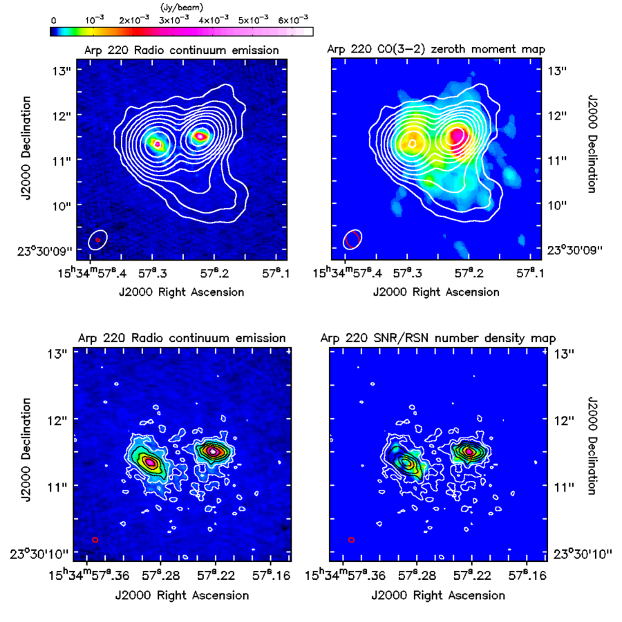
Figure 1.— Radio emission from Arp 220 at 6 and 33 GHz. (a) 33 GHz image (FWHM resolution of 0$\farcs$081 $\times$ 0$\farcs$063, p.a. $\approx$ 65^∘) with 6 GHz contours overlaid (FWHM resolution of 0$\farcs$48 $\times$ 0$\farcs$35, p.a. $\approx$ -40^∘).The contours are in factor of 2 step, with the outermost contour corresponding to $12.5\sigma$, where $\sigma$ = 14 $\mu$Jy beam^-1, and enclosing 98% of the total flux density. In the lower left corner, we show the FWHM of the clean beam for the 33 GHz (red) and 6 GHz (white) image. (b) The same 6 GHz contours overlaid on the CO(3$\to$2) integrated intensity map of Sakamoto et al. (2008) (FWHM resolution of 0$\farcs$38 $\times$ 0$\farcs$28, p.a. $\approx$ 23^∘). In the lower left corner, we show the FWHM of the clean beam for the 33 GHz (red) and CO(3$\to$2) (white) image.(c) A 33 GHz radio continuum image with its contours overlaid. The contours are in factor of 2 step, with the outermost contour corresponding to $3\sigma$, where $\sigma$ = 23 $\mu$Jy beam^-1, and enclosing 97% of the total flux density. (d) 33 GHz contours overlaid on a radio supernova (RSN) and/or supernova remnant (SNR) number density map constructed using the point sources found by Lonsdale et al. (2006). We clearly resolve structure surrounding both nuclei and see a broad similarity between the radio continuum, gas traced by CO, and recent RSNe and/or SNRs.

3. Results

In Figures 1 and 2, we present new VLA images of Arp 220 at 6 and 33 GHz and the radial profiles of each nucleus at 33 GHz. Using these new data, combined with a CO (3$\to$2) integrated intensity (“zeroth moment”) map from Sakamoto et al. (2008), and positional information of point sources found by Lonsdale et al. (2006), we carry out a series of calculations to determine what mechanism is producing most of the radio emission, how radio emission traces recent star formation, and the true sizes and shapes of the nuclear disks. In Tables 1, 2 and 3 we present the results of these calculations.

3.1. Integrated Flux Densities and Spectral Indices

Table 1Flux Densities and Spectral indices for Arp 220

Frequency	Total	East nucleus		West nucleus
(GHz)	(mJy)	Integrated (mJy)	Peak (mJy beam-1)	Integrated (mJy)	Peak (mJy beam-1)
4.7	222.0 $\pm$ 1.9	92.4 $\pm$ 2.1	61.8 $\pm$ 0.5	114.6 $\pm$ 4.3	89.5 $\pm$ 0.7
7.2	171.4 $\pm$ 2.3	73.2 $\pm$ 1.4	36.0 $\pm$ 0.4	89.5 $\pm$ 1.4	60.4 $\pm$ 0.7
5.95	197.6 $\pm$ 2.8	81.4 $\pm$ 2.8	49.0 $\pm$ 0.7	94.3 $\pm$ 1.7	73.3 $\pm$ 1.0
32.5	61.8 $\pm$ 7.2	30.1 $\pm$ 3.9	4.1 $\pm$ 0.5	33.4 $\pm$ 4.0	6.5 $\pm$ 0.8
Spectral index
$\mathrm{\alpha_{6-33GHz}}$	-0.69 $\pm$ 0.07	-0.59 $\pm$ 0.08		-0.61 $\pm$ 0.07
$\mathrm{\alpha_{4.7-7.2GHz}}$	-0.61 $\pm$ 0.04	-0.55 $\pm$ 0.07		-0.58 $\pm$ 0.09

Note. — For details on the calculations, see Section 3.1

In Table 1, we report the flux density of the entire system, each nucleus, and the resulting spectral indices. We used a curve of growth method to derive the flux densities. For the integrated flux density, we progressively $(u,v)$ tapered and re-imaged the data, recording the total flux density above a signal-to-noise of 5 at each resolution. These flux densities agree with those measured from the imaging of individual arrays (see Section 2). For the flux densities of the individual nuclei, we used CASA’s imstat task to place circular apertures around each component, varying their radii. We plotted the flux density against aperture radius and looked for convergence in this curve-of-growth to identify the true flux density. We also independently measured the integrated flux of the south-west component seen at C band (see Figure 1a), using an aperture in the CASA viewer, and found that it encloses $\sim$ 3% of the total 5.95 GHz flux density. The integrated flux densities at both frequencies agree, within the reported errors, with predicted values based on the modeled integrated SED published in the literature (e.g., Anantharamaiah et al., 2000).

Using these flux densities, we calculated the spectral indices, $\alpha$ for $\mathrm{F_{\nu}\propto\nu^{\alpha}}$, of the whole system and each nucleus via

$$\alpha_{1-2}=\frac{\log F_{1}-\log F_{2}}{\log\nu_{1}-\log\nu_{2}}~{},$$ (1)

where $F_{1}$ and $F_{2}$ are the flux densities at frequencies $\nu_{1}$ and $\nu_{2}$. Equation 1 will be valid for flux densities $\mathrm{F_{1}~{}and~{}F_{2}}$ over matched apertures (or for integrated values over whole systems).

3.2. Comparison to Gas and Recent Star Formation

To assess the degree to which the measured sizes are characteristic of the whole system, we compared our maps to known distributions of emission from gas and recent radio supernovae and/or supernova remnants (RSNe/SNRs). In Figure 1b, we plot C band contours over the CO (3$\to$2) map of Sakamoto et al. (2008) (restoring Gaussian beam with FWHM 0$\farcs$38 $\times$ 0$\farcs$28 at a p.a $\approx$ 23^∘).

The RSNe/SNRs trace recent star formation, and they can accelerate cosmic ray (CR) electrons that emit synchrotron radiation. We built a map of RSN/SNR number density from the locations of 49 point sources identified by Lonsdale et al. (2006) from 18 cm VLBI observations. On our 33 GHz astrometric grid, we convolved delta functions with a fixed, fiducial intensity at the positions of the point sources with our 33 GHz beam. In Figures 1c and 1d, we compare the 33 GHz map to the distribution of recent RSNe/SNRs.

Note that although we use RSNe/SNRs as signposts of recent star formation, the VLBI sources do not contribute significantly to the flux that we observe. For a typical synchrotron spectral index $\alpha_{\rm 1.7-33GHz}=-0.7$, the Lonsdale et al. (2006) RSNe/SNRs would contribute 1.5 mJy at 33 GHz and 4.9 mJy at 6 GHz. This contribution would only account for $\sim$ 2.5 % of the total flux density that we observe with the VLA. Even at 18 cm, the Lonsdale et al. (2006) RSNe/SNRs have integrated flux only $\sim$ 12 mJy at 18 cm, or $\sim$ 4% of the total flux density of Arp 220 at that frequency (Williams & Bower, 2010). This contribution is small compared to the 10% expected fraction in normal spiral galaxies like M31 or the Milky Way (Pooley, 1969; Ilovaisky & Lequeux, 1972). This difference is most likely due to free-free absorption at 18 cm (see Section 4.3.4).

3.3. The Morphology of Arp 220 nuclei at 33 GHz

Table 2Best-Fit Morphology for the Nuclei of Arp 220 at 33 GHz

Parameter	East nucleus		West nucleus
	Deconvolved	Convolved	Deconvolved	Convolved
Exponential Disk Model
Scale length (pc)	30.3 $\pm$ 4.6	34.0 $\pm$ 5.1	21.0 $\pm$ 3.2	25.4 $\pm$ 3.8
Peak intensity (mJy beam-1)	6.0 $\pm$ 0.7	4.8 $\pm$ 0.6	13.4 $\pm$ 1.6	9.0 $\pm$ 1.1
Position angle ($\arcdeg$)	54.7 $\pm$ 0.6	55.4 $\pm$ 0.6	79.4 $\pm$ 0.8	77.3 $\pm$ 0.8
Inclination ($\arcdeg$)	57.9 $\pm$ 0.6	55.4 $\pm$ 0.6	53.5 $\pm$ 0.5	49.1 $\pm$ 0.5
$\mathrm{R_{50}}$ (pc)	50.8 $\pm$ 7.6	57.0 $\pm$ 8.6	35.2 $\pm$ 5.3	42.7 $\pm$ 6.4
Two Dimensional Gaussian Fitting
FWHM major axis (pc)	85.9 $\pm$ 8.6	90.8 $\pm$ 9.1	63.7 $\pm$ 6.4	70.2 $\pm$ 7.0
FWHM minor axis (pc)	46.3 $\pm$ 4.6	51.8 $\pm$ 5.2	38.0 $\pm$ 3.8	44.7 $\pm$ 4.5
Position angle (∘)	56.0 $\pm$ 1.1	56.5 $\pm$ 1.1	78.7 $\pm$ 1.6	77.1 $\pm$ 1.5
Observed Half-Light Radius
$\mathrm{R_{50sky}}$ (pc)		73.3 $\pm$ 7.5		45.5$\pm$ 3.7

Note. — The reported parameters were obtained by fitting a 2-D exponential and Gaussian distribution, respectively. The quoted uncertainties reflect the systematic uncertainty from varying the goodness of fit statistic or other methodology in the fit. In the case of the peak intensity, the uncertainty is determined by the flux density calibrator error,  12%. In all cases, the errors from the fit are negligible. For Arp 220 ($d_{L}$ = 77 Mpc), 10 pc $\approx$ 0$\farcs$03 or 0$\farcs$1 = 36.9 pc

The smooth, ellipsoidal isophotes in Figure 1 suggest a disk-like geometry. We modeled the 3 $\sigma$ clipped image of Arp 220 at 33 GHz (outermost contour in Figure 1c) using a 2-D non-linear least-squares fitting technique. After experimenting with Gaussian, exponential, Sérsic and hybrid profiles, we found that the two disks are reasonably described by thin, tilted exponential disks. We fit both nuclei simultaneously by varying, without constraints, the amplitude, position angle (p.a.), inclination, center, and scale length of each nucleus. Although the parameters did not have constraints, the starting points were educated guesses of the final parameters. In each case, we construct the model image, convolve it with the synthesized beam of our observations, and compare the model and observed intensities to derive $\chi^{2}$. Note that the results for the inclination of the disks represent lower limits because we assume thin disks.

The best fit parameters from the model fitting, along with associated uncertainties, are reported in Table 2. In addition to deriving formal uncertainties, we gauge the accuracy of our fit by varying our approach among several reasonable methods. For example, we adopt a logarithmic, rather than linear, goodness of fit statistic and we fit the radial profile rather than the image itself. These imply an uncertainty of $\approx 15\%$ for the scale length and a few percent for p.a. and inclination. The error in the normalization is dominated by our overall uncertainty in the amplitude calibration ($\approx 12\%$). As another point of comparison, we also report the results of simple Gaussian fitting, although, we emphasize that the residuals are substantially poorer for this approach at low and high radius.

From the exponential model, we obtain deconvolved scale lengths of $30$ and $21$ pc for the east and west nucleus, respectively. Our results for p.a., inclination, and center did not vary significantly with the choice of functional form. While the fits appear to be good descriptions, they are not perfect. From the residual images, we found that the western nucleus showed higher residuals in the disk than the eastern nucleus, while the center of the eastern nucleus had higher residuals than the western nucleus.

Both nuclei are well resolved, showing significant extent compared with the synthesized beam. The implied deconvolved half-light radii, ${\rm R_{50d}}$, are $51$ and $35$ pc, respectively; that is, if viewed face-on, we would expect half the emission from Arp 220 to come from nuclear disks $\sim 100$ (east) and $\sim 70$ (west) pc across. In Figures 1 and 2, we have also shown that the size measurement agrees with that implied by the RSN/SNR distribution (Lonsdale et al., 2006).

The p.a.’s of the east and west nuclei agree well with those of the kinematic major axes of the disks measured from sub-millimeter CO observations (Sakamoto et al., 1999, 2008), H I absorption observations from Mundell et al. (2001), and $\mathrm{H53\alpha}$ radio recombination line Rodríguez-Rico et al. (2005). The velocity gradients along these position angles on individual nuclei have also been observed in the 2 $\mu$m $\mathrm{H_{2}}$ line (Genzel et al., 2001) which traces hot molecular gas and 2.3 $\mu$m CO absorption (the latter traces stellar velocities: (Engel et al., 2011)).

We performed two checks on the size measurements. First, as a point of comparison, we report in Table 2 a 2-D Gaussian fit to each nucleus at 33 GHz. We obtained deconvolved FWHM sizes of 0$\farcs$23 $\times$ 0$\farcs$13 ($\mathrm{86~{}\times~{}46~{}pc^{2}}$) for the eastern and 0$\farcs$17 $\times$ 0$\farcs$10 ($\mathrm{64~{}\times~{}38~{}pc^{2}}$) for the western nucleus. These sizes agree fairly well with previous, marginally resolved, estimates at other frequencies. Downes & Eckart (2007) found a deconvolved major axis size of 0$\farcs$19 = 70 pc for the western nucleus at 1.3 mm. Sakamoto et al. (2008) found major axis sizes of 0$\farcs$27 = 100 pc (FWHM, east) and 0$\farcs$16 = 59 pc (FWHM, west) at 860 $\mu$m. However, we show through radial profiles (Figure 2) that the disks are better described by an exponential morphology. In fact, the deconvolved Gaussian fit would underestimate the deconvolved half-light diameter of the disks by 9 %(west) and 15% (east), if we account for inclination effect in the gaussian fit, i.e, the deconvolved $\mathrm{FWHM_{major}}$ is smaller by $\sim$ 9% and 15% when compared to the deconvolved half-light diameter ($2\times{\rm R_{50d}}$).

Second, we calculated the area on the sky containing half of the flux associated with each nucleus. This very basic measure still suffers from beam dilution and inclination effects, but provides a measure of size that is independent of the functional form. We derived this image-based $A_{\rm 50sky}$ by identifying the isointensity contour that encloses 50% of the total flux density of each nucleus. We summed the area of the pixels (pixel size = 0$\farcs$02) enclosed within that contour and estimate the observed radius for $i=55.4\arcdeg$ (east) and $i=49.1\arcdeg$ (west), and $\mathrm{R_{50sky}=\sqrt{A_{50sky}/(\pi~{}\cos i)}}$. This is $\sim$ 73 pc for the eastern nucleus and $\sim$ 46 pc for the western nucleus. We report the observed ${\rm R_{50sky}}$ values in Table 2. As with the Gaussian, the measured area shows broad agreement with the exponential profile fitting, though differing in detail.

We created deprojected, azimuthally averaged radial profiles of 33 GHz intensity to assess the accuracy of our models and compare the structure of the nuclei to that of the RSN/SNR number density map. Assuming a thin tilted ring geometry, we calculated deprojected profiles for the observed emission, the emission in the convolved model, and the RSN/SNR number density map. In each case, the center of the profiles correspond to the highest intensity pixel in the observed image for each nucleus. We plot these profiles in Figure 2. We included only emission above a signal-to-noise ratio of 3 and then averaged the intensity in a series of inclined, $\sim$0$\farcs$035-wide (half the clean beam size) rings, adopting the best-fit model inclination and p.a. from our modeling (Table 2). Note that these rings oversample the $\sim$ 0$\farcs$07 beam, so that adjacent bins in Figure 2 are not independent. We normalized the RSN/SNR radial profile to match the 33 GHz profile at $r\approx 0\farcs 09$. The plotted error bars were calculated from the standard deviation of the flux within each annulus divided by the square root of the area in that annulus expressed in units of the beam size (i.e., the number of independent beams).

In Figure 2, we show that the exponential model matches the data well for both nuclei, matching slightly better for the western nucleus. Meanwhile, the Gaussian profile is not as good as the exponential profile when compared to the observed data, being particularly poorer in the outer parts of the disks. The linearity of the semilog profiles also confirms (and motivates) our adoption of an exponential functional form. The RSN/SNR radial profiles mostly follow the integrated radio emission profiles (and thus also the model). The agreement is better in the western nucleus. The eastern nucleus lacks a bright central peak and shows a somewhat more scattered distribution, which could be caused by stochasticity and timescale effects; i.e., there just may not be enough RSNe/SNRs visible to give a smooth appearance (compare to Figure 1d to see the clumpy nature of the SNe distribution). The same idea applies for the outskirts of the western nucleus. In the rest of the paper, we will consider that the RSN/SNR number density distribution follow the continuum emission observed at 33 GHz closely enough that we can take our measured 33 GHz sizes as indicative of the distribution of active star formation in Arp 220.

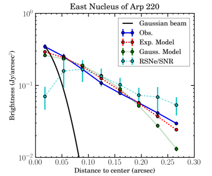
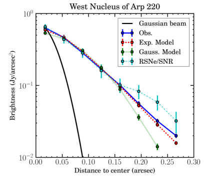
Figure 2.— Azimuthally averaged radial profiles for the deprojected image of the east nucleus (left) and west nucleus (right) in semilog space. Blue solid curves are 33 GHz emission, and cyan dotted dashed line curves are the RSN/SNR number density profiles scaled to match the 33 GHz radial profile at 0$\farcs$09. Red dotted lines and green dashed lines are the radial profiles of the exponential and Gaussian model images, respectively, convolved with the beam. The black solid lines represent the Gaussian beam radial profile.

3.4. Brightness Temperatures

Table 3Average Brightness Temperatures in Arp 220

Frequency	Total system	East nucleus	West nucleus
(GHz)	Log[$T_{b}$(K)]	Log[$T_{b}$(K)]	Log[$T_{b}$(K)]
5.95	4.64 $\pm$ 0.07	4.43 $\pm$ 0.10	4.81 $\pm$ 0.10
32.5	2.7 $\pm$ 0.1	2.5 $\pm$ 0.1	2.9 $\pm$ 0.1

Note. — Integrated values are calculated within ${\rm A_{50d}}$ (deconvolved modeled size) at 33 GHz (more in Section 3.4). The uncertainties follow from propagation of uncertainties quoted earlier in this paper.

The brightness temperature, ${\rm T_{b}}$, can be used to constrain the emission mechanism and energy source, and may give clues regarding the optical depth. With well resolved sizes, we can circumvent beam dilution that often confuses estimates of ${\rm T_{b}}$. We calculated ${\rm T_{b}}$ using the Rayleigh-Jeans approximation via

$$T_{b}=\Big{(}\frac{S_{\nu}}{\Omega_{source}}\Big{)}\frac{c^{2}}{2k_{B}\nu^{2}}~{},$$ (2)

with $S_{\nu}$ the flux density at frequency $\nu$ and $\Omega_{source}$ the area subtended by the source.

We report average Rayleigh-Jeans brightness temperatures, $T_{b}$, in Table 3. From our model, we take the area $\mathrm{A_{50d}\equiv\pi R_{50d}^{2}}$ that we expect to enclose half the emission if the system were viewed face on (see the “deconvolved” column in Table 2). Assuming this to be the true area of the disk at all frequencies, we derive average ${\rm T_{b}}$ over the half-light region. This means we used half of the observed flux density for ${\rm S_{\nu}}$ and ${\rm A_{50d}}$ for ${\rm\Omega_{source}}$ in Equation 2. Our rationale for this assumption is that the 33 GHz image appear to be optically thin, high-resolution tracer of the distribution of recent star formation. Assuming that this structure is common across wavelength regimes allows us to use a “true” size in place of a size observed with a much coarser beam. We also calculated the peak ${\rm T_{b}}$ at each band from the peak flux density and the area of the clean beam at each frequency. This peak ${\rm T_{b}}$ is higher at 33 GHz than at 6 GHz; this simply reflects that the area of Arp 220 at 33 GHz is smaller than the beam size at 6 GHz. For exactly this reason — the small size of Arp 220 and the variable resolution at different frequencies — the peak measurement has limited utility and we only report the “average” version.

The average ${\rm T_{b}}$ is from $10^{4.4}$ K at 6 GHz to $10^{2.5}$ ($\approx 300$) K at 33 GHz, for the east nucleus and $10^{4.8}$ K at 6 GHz to $10^{2.9}$ ($\approx 800$) K at 33 GHz, for the west nucleus.

4. Discussion

Figure 1 shows that our observations clearly separated the nuclei at both 6 and 33 GHz and resolve the structure of both nuclei is resolved at 33 GHz. We find a projected nuclear separation of 0$\farcs$96 $\pm$ 0$\farcs$01 (354 $\pm$ 4 pc), in agreement with previous works (e.g., Scoville et al., 1998; Soifer et al., 1999; Rodríguez-Rico et al., 2005; Sakamoto et al., 2008). In the following subsections, we discuss the radio continuum emission processes, the correspondence with gas and dust emission, and consequences of the small sizes of the emission regions. There is a large scale agreement between the locations of radio continuum emission, CO, and RSNe/SNRs, suggesting that the sizes of the radio continuum sources may be viewed as characteristic of the system.

4.1. Synchrotron Produces Most of the 33 GHz Emission

Synchrotron radiation appears to produce most of the continuum emission at both 6 and 33 GHz. The high brightness temperature of a few $\times$ $10^{4}$ K, inferred at 6 GHz by using the 33 GHz nuclear sizes, argues in this direction. This high brightness temperature cannot come from Hii regions, even if they are completely opaque, because in a purely thermal environment, the electron temperature of such regions should not exceed $10^{4}$ K. If we combined the high brightness temperature with the observed internal C band spectral index of the total system, $\alpha_{\rm 4.7-7.2GHz}=-0.61\pm 0.04$, we infer that most of the emission at 6 GHz is synchrotron.

The spectral index between 6 and 33 GHz, $\alpha_{\rm 6-33GHz}=-0.69\pm 0.05$, matches the internal C band $\alpha$ of the total system within the errors; the same is true for the two nuclei separately (see Table 1). The similarity between $\alpha_{\rm 4.7-7.2GHz}$ and $\alpha_{\rm 6-33GHz}$ indicates no significant spectral flattening between 6 and 33 GHz, suggesting that synchrotron dominates the emission across this range of frequencies. Reinforcing this point, our total flux density and spectral index agree with the predictions made by Anantharamaiah et al. (2000) (see their Figure 10b). They found synchrotron emission to dominate below $\sim 60$ GHz, and estimated the thermal fraction at 6 GHz and 33 GHz to be $\sim$ 15% and 35%, respectively. If we assume a non-thermal spectral index of $-0.76$ (see Table 9 in Anantharamaiah et al., 2000) and a typical thermal spectra index of $-0.1$, we obtain $\alpha_{\rm 6-33GHz}\approx-0.62$ and $\alpha_{\rm 4.7-7.2GHz}\approx-0.65$, which is consistent with what we measure and with our observation of a constant spectral index from 6 to 33 GHz. This result is also consistent with previous results showing lower thermal fractions at 33 GHz for merging starbursts compared to normal galaxies (Murphy, 2013).

The overall star formation rate of the system provides an alternate way to estimate the expected thermal radio continuum emission. Beginning with the IR (8 to 1000 $\mu$m) luminosity of Arp 220, we estimate the expected thermal luminosity of the system if the IR is all due to star formation by following star formation rate conversions from Table 8 in Murphy et al. (2012) and assuming an electron temperature of 7500 K (Anantharamaiah et al., 2000). This approach predicts a thermal fraction of $\sim$ 55% at 33 GHz and $\sim$ 20% at 6 GHz. This is in good agreement with the thermal fraction at 33 GHz obtained in Condon (1992) for a prototypical starburst, M82. However, if we derive the expected spectral index as we did at the end of the previous paragraph (assuming 55% of thermal fraction at 33 GHz), we obtain $\alpha_{\rm 6-33GHz}\approx-0.42$ and $\alpha_{\rm 4.7-7.2GHz}\approx-0.63$, which deviates considerably from what we observe between 6 and 33 GHz. Note that $\alpha_{\rm 4.7-7.2GHz}$ does not vary significantly from what we observe, this is due to the small thermal fraction expected at this frequency range.

The easiest explanation for the lower-than expected thermal flux is that a significant fraction of the ionizing photons produced by young stars are absorbed by dust before they produce ionizations. This would lower the free-free estimate in the calculation. We estimate that to match our observations, we would require that at least 20% of the ionizing photons be absorbed by dust. This number seems plausible for an environment as dust embedded as Arp 220 (see Section 4.3.4) and is consistent with some of the arguments made when considering the apparent deficit of IR cooling line emission (Díaz-Santos et al., 2013, and references therein). Alternatively, an IMF that produces more bolometric light (and thus IR and likely SNe) relative to ionizing photons could resolve the discrepancy. That is, we could invoke an “intermediate-heavy” IMF compared to that used in Murphy et al. (2012). We could also reconcile our two estimates if the synchrotron spectral slope decays drastically between 6 and 33 GHz, so that the apparent 33-6 GHz index is a combination of very steep, curving synchrotron and emerging thermal emission. However, this would require that thermal emission make up most of the SED at higher frequencies, which is not observed (see Anantharamaiah et al., 2000; Clemens et al., 2010).

Our best interpretation of the data is that the 33 GHz emission is mostly synchrotron, in mild contrast with a typical starburst galaxy (see Figure 1 in Condon, 1992). We suggest that the most likely cause is the suppression of thermal radio emission as dust absorbs ionizing photons.

4.2. The Radio Emission Coincides with Gas, Hot Dust and RSN/SNR

In Figure 1b, we show the 6 GHz emission is largely co-spatial with CO emission. The 6 GHz emission is our more sensitive band, with a beam nearly matched to the CO, and — as just discussed — we expect that it traces the same synchrotron emission as the 33 GHz. The CO and 6 GHz emission cover roughly the same area, have broadly coincident peaks, and both show an extended faint feature to the southwest (Mazzarella et al., 1992, note a similar coincidence between 18cm emission and the Arp 220 starburst traced in the near-IR). The distributions of CO and 6 GHz emission do significantly differ in detail. The ratio of fluxes for the two nuclei is 1:2 (east:west) for CO and almost 1:1 for continuum. In the west nucleus, the morphology is more centrally concentrated at 6 GHz compared to the CO map. Some of these differences may reflect real differences between the current gas reservoir and recent star formation, but they may also reflect temperature and optical depth effects. The CO (3$\to$2) emission in this region shows good evidence for optical thickness (Sakamoto et al., 2008), and the densities are high enough that the gas temperature will be likely coupled to the dust ($\sim 100$ K).Therefore, making a straightforward interpretation of the CO in terms of column density is challenging. We draw the broad conclusion from Figure 1b that the synchrotron originates from the same region as, and in very rough proportion to, the molecular gas supply.

A similar situation is also observed on smaller spatial scales by the comparison of the RSN/SNR number density map to the 33 GHz map (see Figure 1d). The distributions are co-spatial, but the continuum map appears smoother than the map made from individual RSN/SNR. This is particularly evident in the eastern nucleus, where the covering fraction of VLBA point sources is small — perhaps a result of stochasticity in the rate and lifetime of SN visible using VLBI measurements. The radial profiles in Figure 2 highlight the quantitative agreement between the continuum and the RSNe/SNRs distribution even more. After azimuthal averaging, the VLBA point source maps are a fairly close match to the 33 GHz continuum.

Such a close match between the 33 GHz continuum extent and the RSN/SNR number density map may not be too surprising: if synchrotron radiation arises from cosmic ray (CR) electrons accelerated by SN shocks, then the 33 GHz continuum emission might be expected to resemble a “puffed up” version of the RSN/SNR distribution due to the diffusion of CR electrons. Instead the distributions match quite well, consistent with most of the 33 GHz emission coming from very close to the original RSN/SNR and little diffusion or secondary CR electron production. This lack of significant propagation could be explained by the cooling timescales being much smaller than the diffusion time. This is expected in compact starbursts with magnetic fields of the order of a mG (see measurements from Robishaw et al., 2008; McBride et al., 2014, based on Zeeman splitting of OH megamaser emission), like Arp 220 (see Figure 1 in Murphy, 2009), though not in normal galaxies (Murphy et al., 2006). For Arp 220, the cooling time of CR electrons at 33 GHz is $\sim$$\mathrm{10^{3}~{}yr}$, which is a combination of synchrotron, bremsstrahlung, ionization and inverse Compton (IC) losses. We make use of Equation 7 in Murphy (2009) for CR electrons with energies greater than 1 GeV to estimate that the synchrotron emitting electrons at 33 GHz only have time to propagate about 5 pc, which is about 1/10th of the size that we have measured for the nuclei. This short diffusion scale yields a synchrotron image that looks very similar to the sites of original CR production (the RSN/SNR) and thus the sites of active star formation. The advantage of the VLA continuum in this case is that in exchange for coarser native resolution, we achieve sensitivity to most of the flux and spatial scales of interest (and potentially still probe a longer timescale).

The similarity of 6 GHz, 33 GHz, CO surface brightness, and the RSN/SNR number density distributions lead us to view our 33 GHz measurement as indicative of the true size of the main disks of star formation and, presumably, gas and hot dust. These morphologies are also consistent with the nuclear morphologies measured in mid-IR with the Keck telescope (Soifer et al., 1999). Perhaps surprisingly, the two disks appear fairly similar in terms of profile, scale length, and observed flux. The western nucleus appears hotter and more compact but the differences are small factors, not an order of magnitude. The physical interpretation of such similarities is unclear. Possible explanations include a similarity in the progenitors, or some “loss of memory” during the process of funneling gas to the center of the galaxies during the ongoing interaction.

4.3. The Nuclear Disks are the Most Extreme Starburst Environments in the Local Universe

4.3.1 Gas Surface Densities

Current best estimates of the dynamical mass per nucleus are $\sim 6\times 10^{9}$ M_⊙ within $\sim 100$ pc of each nucleus (Engel et al., 2011). These values are still uncertain, with $\sim 2\times 10^{9}$ M_⊙ representing a likely lower limit in both nuclei (Engel et al., 2011). The dynamical mass represents an upper limit on the gas content. Based on dynamical modeling and CO imaging, Downes & Solomon (1998) estimated the gas content at $1.1\times 10^{9}$ and $0.6\times 10^{9}$ M_⊙ for the eastern and western nucleus, but embedded in a larger gas disk with total mass $\sim 3\times 10^{9}$ M_⊙ (see also Sakamoto et al., 1999, 2008; Downes & Eckart, 2007). These estimates mix dynamical modeling with observations of low-J CO line (up to J = 3$\to$2) measurements that are likely very optically thick in Arp 220. Papadopoulos et al. (2012) provide an alternative, but unresolved, estimate by focusing on higher J CO transitions and high critical density tracers (e.g., HCN) to estimate a total molecular gas mass of $\mathrm{\sim(15-28)\times 10^{9}~{}M_{\odot}}$ for the entire system. The difficulty with this estimate is apportioning this gas mass to the various components of the system. We consider a conservative approach to be the following: we assume that half of the total molecular gas mass is equally distributed between the two nuclei and the other half in an outer disk (e.g., see Sakamoto et al., 1999, for evidence of an outer disk). This implies $\sim 3.5$–$7\times 10^{9}$ M_⊙ of gas per nucleus from Papadopoulos et al. (2012). This remains in moderate tension with the dynamical masses because it would imply very high gas fractions, but given the mismatch in scales (the dynamical masses are estimated on $\sim 100$ pc scales) and uncertainties in modeling, a factor of $\sim 3$–$5$ uncertainty seems plausible (Sakamoto et al., 2008).

The areas that we measure for the Arp 220 nuclei are stunningly small, especially when compared to the integrated properties of the system. We adopt the literature gas mass of the nuclei as $3.5^{+3.5}_{-1.5}\times 10^{9}$ M_⊙, with the lower bound set by the Engel et al. (2011) values, the upper bound set by Papadopoulos et al. (2012), and the best estimate consistent (with modest tension) with the latter. We further expect half of the gas mass of each to be distributed within the half-light deconvolved, face-on, area (${\rm A_{50d}}$) of our radio images (these trace star formation, so we implicitly assume that gas and star formation track one another within the system). We thus compare $\sim 1.75^{+1.75}_{-0.75}\times 10^{9}$ M_⊙ to our half-light areas to estimate average, nuclear, gas surface densities. The deprojected, deconvolved gas surface densities are $2.2^{+2.1}_{-1.0}\times 10^{5}$ M_⊙ pc^-2 (east) and $4.5^{+4.5}_{-1.9}\times 10^{5}$ (west) M_⊙ pc^-2. These translate to an average, nuclear, total hydrogen column densities of $2.7^{+2.7}_{-1.2}\times 10^{25}$ cm^-2 (east) and $5.6^{+5.5}_{-2.4}\times 10^{25}$ cm^-2 (west) (divide these numbers by 2 for H₂ column densities). These nuclear hydrogen columns are $\sim 3$–$4$ orders of magnitude higher than those derived from X-ray observations (e.g., Clements et al., 2002; Iwasawa et al., 2005), but they roughly agree with those derived from observations at $860~{}\mu$m (Sakamoto et al., 2008) and $434~{}\mu$m (Wilson et al., 2014). The gas surface densities that we derive roughly resemble the maximum stellar surface density of $\sim 10^{5}$ M_⊙ pc^-2 found in a compilation of literature data by Hopkins et al. (2010). Given the large uncertainty in our mass estimate (and the scatter in the Hopkins et al. (2010) compilation) Arp 220 appears consistent with producing such a “maximal” stellar surface density system. This is especially true when one considers that feedback and further evolution of the system may reduce the efficiency (final fraction of gas converted to stars) in the nuclei below unity (a factor of $\sim 1/3$ would produce excellent agreement).

We do not know the thickness of the disks, but by adopting a spherical geometry we can calculate a lower limit to the H₂ particle densities in the nuclei. This is $3.8^{+3.8}_{-1.6}\times 10^{4}$ cm^-3 (east) and $11^{+12}_{-4.5}\times 10^{4}$ cm^-3 (west). For comparison, a typical Milky Way molecular cloud has a surface density $\sim 100$ M_⊙ pc^-2 (N(H)$\sim 10^{22}$ cm^-2) and average particle density ${\rm n_{H_{2}}\sim 100~{}cm^{-3}}$. In addition to faster free fall times, correspondingly more efficient star formation, and phenomenal opacity, potential implications of such high molecular gas densities would include the secondary production of CR electrons and confinement of CR electrons.

4.3.2 Infrared Surface Densities and Star Formation Rates

By following the same approach, we assume the infrared emission in Arp 220 is coincident within our measured radio distribution and explore the implications. Conventionally, the infrared luminosity surface density, $\Sigma_{\rm IR}$, is defined as the luminosity per unit area of the system. We calculate $\Sigma_{\rm IR}$ by assuming that half of the infrared luminosity (from 8–1000 $\mu$m) is generated within the deconvolved, face-on, half-light area (${\rm A_{50}}$), i.e, we calculate an average infrared luminosity surface density, within the half-light area, via

$$\Sigma_{\rm IR}=\Big{(}\frac{0.5\times L_{IR}[8-1000\mu m]}{A_{50}}\Big{)}=\Big{(}\frac{L_{50}}{A_{50}}\Big{)}~{}.$$ (3)

Following our measurements above, we use $\mathrm{A_{\rm 50d}\equiv\pi(R_{50d,east}^{2}+R_{50d,west}^{2})}$ to derive a total (face on) infrared luminosity surface density of $\mathrm{\Sigma_{IR}\sim 6.0^{+2.3}_{-1.5}\times 10^{13}~{}L_{\odot}~{}kpc^{-2}}$ . If we further assume that the ratio of the fluxes between the east and west nuclei at 33 GHz ($\sim$ 1:1) holds at infrared wavelengths, then using the derived radio $\mathrm{A_{50d}\equiv\pi R_{50d}^{2}}$ for the individual disks, we obtain $\mathrm{\Sigma_{IR}\sim 4.2^{+1.6}_{-0.7}\times 10^{13}~{}L_{\odot}~{}kpc^{-2}}$ and $\mathrm{\Sigma_{IR}\sim 9.7^{+3.7}_{-2.4}\times 10^{13}~{}L_{\odot}~{}kpc^{-2}}$ for the east and west nucleus, respectively. These values are more than an order of magnitude higher than those for the central 0.3 pc of the Orion nebula complex and M 82 ($\mathrm{\sim 2\times 10^{12}~{}L_{\odot}~{}kpc^{-2}}$ and $\mathrm{\sim 9\times 10^{11}~{}L_{\odot}~{}kpc^{-2}}$, respectively (Soifer et al., 2000)), but are closer to those found in the brightest clusters within starburst galaxies ($\mathrm{\sim 5\times 10^{13}~{}L_{\odot}~{}kpc^{-2}}$ (Meurer et al., 1997)). Our estimated surface densities are consistent with Soifer et al. (2000), who estimated infrared luminosity surface densities of $\mathrm{1-6\times 10^{13}~{}L_{\odot}~{}kpc^{-2}}$ based on mid-IR Keck observations and radio data from Condon et al. (1991).

The deprojected SFR surface density (defined as the SFR per unit area in the disk), $\Sigma_{\rm SFR}$, is a close corollary of the IR luminosity surface density. We estimate this quantity within the deconvolved, face-on, ${\rm A_{50d}}$ for each nucleus at 33 GHz, using a 1:1 ratio between east and west, the radio luminosity to SFR conversion from Table 8 in Murphy et al. (2012), and an electron temperature and non-thermal spectral index of 7500 K and 0.76 (the spectral index in Murphy et al. (2012) is defined with the opposite sign compared to our definition), respectively, from Anantharamaiah et al. (2000). We obtain a $\Sigma_{\rm SFR}$ of $\sim$ $10^{3.7\pm 0.1}$ and $10^{4.1\pm 0.1}$ $\mathrm{M_{\odot}~{}yr^{-1}~{}kpc^{-2}}$ within the half-light of the eastern and western nuclei, respectively (divide these numbers by two to take into account both sides of the disks). The total SFR calculated from ${\rm L_{IR}}$, 180 $\mathrm{M_{\odot}~{}yr^{-1}}$, and from the total radio flux density at 33 GHz (${\rm L_{Radio}}$), 195 $\mathrm{M_{\odot}~{}yr^{-1}}$, differ by only $\sim$ 10%, consistent with Arp 220 lying on the (33 GHz) radio-to-far infrared correlation (and meaning that we would obtain essentially the same $\Sigma_{\rm SFR}$ for either luminosity). The radio SFR value differs by 20% from that derived from Anantharamaiah et al. (2000), which we consider to be within the uncertainties of such calculations.

$\Sigma_{\rm IR}$ tells us coarsely about the density of IR luminosity per unit area, but not necessarily the flux at the surface of the source, which may have important implications for feedback and depends on the detailed geometry of the system. A spherical geometry provides a useful limit on the flux at the surface of the system. In this case, $\mathrm{F_{sphere}=L_{50}/(4~{}\pi~{}R_{50d}^{2})}$ will be the flux at the surface of a sphere of radius ${\rm R_{50d}}$ with the luminosity of Arp 220. Using the measured radio sizes, $\mathrm{F_{sphere}\sim 1.5^{+0.6}_{-0.4}\times 10^{13}~{}L_{\odot}~{}kpc^{-2}}$ for the entire system, $\mathrm{\sim 1.1^{+0.4}_{-0.2}\times 10^{13}~{}L_{\odot}~{}kpc^{-2}}$ for the eastern nucleus and $\mathrm{\sim 2.4^{+0.9}_{-0.6}\times 10^{13}~{}L_{\odot}~{}kpc^{-2}}$ for the western nucleus. A less extreme case, one that may well apply to Arp 220, is a two-sided disk. With one half of the luminosity emergent from each side, we have $\mathrm{F_{disk}=L_{50}/(2~{}\pi~{}R_{50d}^{2})}$, twice the spherical case. As one would expect, these values are lower than the simple $\Sigma_{\rm IR}$, but they also differ from one another, reinforcing the importance of geometry to the physics of the source.

Yet another subtlety arises in the specific case where one wishes to calculate the flux through an area very close to, but just above one side of a disk. This quantity is relevant to the often-discussed case of radiation pressure on dust (see Section 4.3.3) but because of projection effects it is not identical to any of the above quantities. In Appendix A, we show that this one-sided flux perpendicular to the disk, which we call $\mathrm{F_{near}}$ is equal to $\mathrm{L_{IR}/(8\pi R_{50d}^{2})}$ (Equation A7) in general. This value is further divided by an extra factor of two for the case of the two nuclei of Arp 220 (because $L_{\rm IR}$ combines the light from the two nuclei). From this calculation, we obtain $\mathrm{F_{near}\sim 1.5^{+0.6}_{-0.4}\times 10^{13}~{}L_{\odot}~{}kpc^{-2}}$ for the entire system (the same as for F_sphere, though not for the same reason), $\mathrm{\sim 1.1^{+0.4}_{-0.2}\times 10^{13}~{}L_{\odot}~{}kpc^{-2}}$ for the east nucleus and $\mathrm{\sim 2.4^{+1.0}_{-0.6}\times 10^{13}~{}L_{\odot}~{}kpc^{-2}}$ for the west nucleus. As discussed in Appendix A, these should be the most appropriate fluxes to consider when assessing the impact of pressure from radiation perpendicular to the disk.

The ratio of the flux densities between the east and west nuclei varies with frequency. Some other ratios for the east:west relation found in the literature include 1:4 at mid-IR (Soifer et al., 1999), 1:3 at 18 cm (if we consider only the contribution of the point sources from Lonsdale et al., 2006) and 1:2 at sub-mm wavelengths (Sakamoto et al., 2008). However, most of these observations do not offer high enough spatial resolution to truly isolate the contribution of each nucleus. If we ignore this issue and we assume a ratio of 1:4, and we use Equation A7, we obtain $\mathrm{F_{near,east}\sim 4.5^{+1.7}_{-1.1}\times 10^{12}~{}L_{\odot}~{}kpc^{-2}}$ and $\mathrm{F_{near,west}\sim 3.7^{+1.4}_{-0.9}\times 10^{13}~{}L_{\odot}~{}kpc^{-2}}$. In every case, we obtain $\mathrm{F_{near}\gtrsim~{}10^{13}~{}L_{\odot}~{}kpc^{-2}}$ for the west nucleus, which is always the higher intensity nucleus.

Note that the same geometric issues discussed here raise a caveat regarding the luminosity of the source, which was derived under the assumption of isotropic emission (Sanders et al., 2003; Sanders & Mirabel, 1996). An optically thick thin disk is not an isotropic emitter. However, neither do our observations constrain the geometry of the infrared photosphere, which is the relevant surface for this calculation. We discuss this issue in Appendix A. Lacking information, we have assumed the isotropic luminosity throughout this paper, but note the uncertainty (see also Downes & Eckart, 2007; Wilson et al., 2014). Note that high angular resolution infrared (from 8–1000 $\mu$m) observations are needed in order to better constrain the true morphology of the IR photosphere of Arp 220.

4.3.3 Radiation Pressure and Maximal Starburst Models

Scoville (2003) and Thompson et al. (2005), argued that for optically thick, dense starburst galaxies, the critical feedback mechanism acting against gravitational collapse, and thus star formation, could be radiation pressure on dust. Although there is ongoing debate about whether or not radiation pressure on dust represents the dominant feedback mechanism in compact starbursts (see Krumholz & Thompson, 2013; Socrates & Sironi, 2013; Davis et al., 2014, for further discussion), the maximal starburst model of Scoville (2003) and Thompson et al. (2005) represents an interesting point of comparison for our present work. In Figure 3, which closely follows Figure 4 of Thompson et al. (2005), we present our new measurements for the flux near the surface of the source (assuming a thin disk geometry, see Section 4.3.2 and Appendix A) in the context of literature observations and predictions by Thompson et al. (2005). The literature observations show a sample of ULIRGs with sizes based on 8.44 GHz radio maps by (Condon et al., 1991) and luminosities from IRAS. Following the approach presented in Appendix A, we calculate F_near following Equation A7 assuming half of the total infrared luminosity to be enclosed within $\mathrm{A_{50}=\pi~{}R_{50}^{2}}$, where $\mathrm{R_{50}}=b_{\rm maj}/2$. We used the deconvolved FWHM major axis, $b_{\rm maj}$, from Condon et al. (1991) in order to account for inclination effects (we only include resolved sources). Following the discussion in the previous section, the fluxes for the points in Figure 3 differs by a factor of 8 compared to those in Thompson et al. (2005). for reasons discussed in Appendix A.

The error bars of our Arp 220 values (filled points in Figure 3) correspond to a combination of the uncertainties in ${\rm R_{50d}}$, and uncertainty in the contribution of each nucleus to the IR luminosity, with the lower/upper limit assuming a ratio of 1:4 between east and west (Soifer et al., 1999). To be conservative, we also assume a 20% uncertainty in the assumption that half of the total IR luminosity is coming from ${\rm A_{50}}$. The plotted values for the flux correspond to $\mathrm{F_{near,east}\sim 1.1^{+0.4}_{-0.8}\times 10^{13}~{}L_{\odot}~{}kpc^{-2}}$ and $\mathrm{F_{near,west}\sim 2.4^{+2.7}_{-0.9}\times 10^{13}~{}L_{\odot}~{}kpc^{-2}}$. In this Figure, we show the “Eddington” values for radiation pressure on dust as solid and dashed lines. These represent an envelope for which radiation pressure on dust balances self-gravity. As a result, no equilibrium star-forming system is expected to exist above this line, hence the “Eddington limit” analogy.

The precise value of the limit depends on the size, gas fraction ($\mathrm{f_{g}}$) stellar velocity dispersion ($\sigma$), Rosseland mean opacity ($\kappa$), and dust-to-gas ratio of the system, leading to the large spread in the model lines seen in the Figure. Our measurements of Arp 220 appear as solid points in Figure 3. There, the west nucleus of Arp 220 appears among the highest brightness systems. However, the west nucleus does not clearly stand out from the other ULIRGs with respect to this value, partially because the more compact size means that the “maximal” value is larger for Arp 220 than for larger systems. Overall, all the systems plotted in Figure 3 lie roughly around the Eddington limit for a f_g = 0.1 and $\sigma$ = 200 km s^-1 disk in Thompson et al. (2005), which is indicated by the blue solid line.

If we adopt $\mathrm{f_{g}=1}$ and $\sigma\approx$ 200 km s^-1 (e.g., Genzel et al., 2001), indicated by the green line in Figure 3, then we calculate a conservative Eddington limit of $\mathrm{\sim 9\times 10^{13}~{}L_{\odot}kpc^{-2}}$ for the west nucleus and $\mathrm{\sim 7\times 10^{13}~{}L_{\odot}kpc^{-2}}$ for the east nucleus. Refined measurements of the geometry, gas fraction, opacity, dust-to-gas ratio and kinematics are needed to specify the models more precisely. For most plausible assumed disk properties, we can say that both Arp 220 nuclei lie well below the Thompson et al. (2005) Eddington-limited starburst value, with the western nucleus being the brightest system among the local ULIRGs. If improved measurements demonstrate one or both nuclei to lie significantly above this value, one would need to consider luminosity sources other than star formation (presumably an AGN Iwasawa et al., 2005; Downes & Eckart, 2007; Rangwala et al., 2011) or question the basic assumptions about geometry and equilibrium embedded in the model, but at present little such tension appears to exist.

Another way to assess the role of radiation pressure in Arp 220 is to assume that radiation pressure does represent the dominant force acting against gravity (see Appendix B) and to calculate the required gas opacity, $\kappa$, of the system in order to be in hydrostatic equilibrium. By following Equation B2, and using the derived values for the gas surface density and the flux for each nucleus (see Section 4.3.1 and 4.3.2), we find that $\mathrm{\kappa_{east}\approx 300~{}cm^{2}/g}$ and $\mathrm{\kappa_{west}\approx 80~{}cm^{2}/g}$ would be required for radiation pressure to balance gravity. Compared to the models from Semenov et al. (2003), which were used in the models from Thompson et al. (2005), these appear to be unrealistically high values for the gas opacity. We interpret these high values as a reinforcement of our previous findings that the nuclei of Arp 220 lie below the dusty Eddington limit for $\mathrm{f_{g}}$ $\sim$ 1 and $\sigma$ = 200 km s^-1 by a factor of $\sim$ 10, and then are not radiation pressure supported.

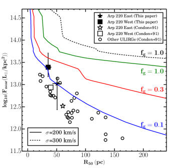
Figure 3.— Flux versus radius for local ULIRGs from Condon et al. (1991) (open symbols), and including the values for the eastern (star symbol) and western (square symbol) nuclei of Arp 220 from this paper (filled symbols). In this figure, we represent a new version of Figure 4 of Thompson et al. (2005). The y-axis corresponds to the flux passing through a surface area near the source, F_near (see Appendix A), and the x-axis to the deconvolved half-light radius. The solid lines represent the Eddington limits for several different gas fractions, $\mathrm{f_{g}}$, assuming stellar velocity dispersion of $\sigma$ = 200 km s^-1. The dashed line shows the model for $\mathrm{f_{g}=1}$ and $\sigma$ = 300 km s^-1. From this figure, we observe that Arp 220 appears among the brightest systems but still well below a conservative dusty Eddington limit described by the green line.

4.3.4 Optical Depth

The small sizes of the Arp 220 nuclei also imply that optical depth effects will be important across the spectrum, even at wavelengths as long as sub-mm. By following the same approach described in Section 3.4, we calculate the average Rayleigh-Jeans brightness temperatures that would be implied by combining the deconvolved half-light sizes of the nuclei with half of the 860 $\mu$m continuum flux densities reported by Sakamoto et al. (2008) from lower resolution observations. At this wavelength, we find implied average brightness temperatures of 19 K (east) and 76 K (west), within the deconvolved half-light area calculated in this paper (${\rm A_{50d}}$), without any accounting for optical depth (which could change the size of the apparent emission). In the west nucleus, this approaches the apparent dust temperature of $\sim 90$ K (see González-Alfonso et al., 2012, for a more thorough idea of the dust temperature in Arp 220), so that optical depth must become important by this wavelength regime, with $\tau\gtrsim 1$ by 860 $\mu$m in the western nucleus. This neglects any more complicated geometric considerations (e.g., see the discussion of an inclined geometry in Downes & Eckart, 2007), which are likely to make the situation even more confused. Optical depth effects appear less severe by $\lambda\sim 1$ mm, combining ${\rm A_{50d}}$ with half of the western nucleus dust emission from Downes & Eckart (2007), implies an average $\mathrm{T_{b}^{1mm}}\sim$ 45 K within the half-light area. This modest mm optical depth is consistent with measurement of a spectral index steeper than $\alpha=2$ by Sakamoto et al. (2008), implying somewhat optically thin emission.

Even this simple calculation demonstrates that by sub-mm wavelengths optical depth effects cannot be neglected, especially in the western nucleus. As a result, we would expect high resolution but higher frequency observations, e.g., at sub-mm wavelengths with ALMA, to observe a moderately optically thick “photosphere” around the galaxy and so recover a larger size than we find here (e.g., see the continuum observations by Wilson et al., 2014). Similarly, line observations at these wavelengths will need to consider the effects of a moderately optically thick sub-mm continuum in their interpretation.

Further, we can estimate the optical depth at 33 GHz. The brightness temperature calculated for the entire source at 33 GHz is $\sim$ 500 K (see Table 3). The thermal fraction at this frequency is $\sim 35$%, so that ${\rm T_{b}}$ of the thermal emission is $\sim$ 175 K. The thermal electron temperature (${\rm T_{e}}$) cannot exceed $\approx 10^{4}$ K because line cooling is high at such high temperatures. Then taking ${\rm T_{e}\sim 10^{4}}$ K and a measured $\sim 175$ K brightness, we estimate the average 33 GHz free-free opacity within the half-light radius to be $\mathrm{\tau_{Thermal}\sim T_{b}/T_{e}\sim 0.018}$. Given that $\mathrm{\tau_{Thermal}\propto\nu^{-2.1}}$, we can calculate that $\mathrm{\tau_{Thermal}\sim 1}$ at $\nu$ $\sim$ 5 GHz. At 18 cm, $\mathrm{\tau_{Thermal}>9}$, which might help explain the low VLBA flux density from Lonsdale et al. (2006). In addition, as Sakamoto et al. (2008) note, the dust opacity is close to unity at 860 $\mu$m. Thus, the Arp 220 nuclei may be transparent only near the middle of the frequency range 5 GHz to 350 GHz. A case can thus be made that the 33 GHz image presented here is the only existing image that is both optically thin and resolves the nuclei.

4.4. Evidence at Radio Wavelengths of a Dominant AGN in the Western Nucleus

In our observations, the western nucleus is more compact with a higher ${\rm T_{b}}$ than the eastern nucleus. However, consistent with previous VLBI observations, we observe no significant central excess in either Arp 220 images or radial profiles (Figures 1 and 2). Parra et al. (2007) discuss the possibility that one of three VLBI point sources showing a flat spectrum ($\alpha>-0.5$), could be an AGN. However, that is one of several possibilities that could explain the shape of their spectrum.

Most of the 33 GHz emission that we observe comes from the compact, but still resolved, disks around the nuclei. Specifically, the nuclear beam of the west nucleus contains 20% of the total flux of the nucleus, while the other 80% arises from the more extended star forming regions (Table 1). Our measured ${\rm R_{50d}}$ contain similar information (see Table 2). We cannot rule out an AGN in the western nucleus, but if one is present it does not make a dominant, point-like contribution to the overall 33 GHz emission on scales of $\approx 30$ pc. Similarly, Arp 220 does not exceed the “Eddington” value that might eliminate star formation as a viable power source (see Section 4.3.3). Smith et al. (1998) show that the SN rate and luminosity of Arp 220 are broadly consistent with emission only generated by star formation, though uncertainty in the IMF, SN rate, and SFR certainly would still allow an AGN contribution.

No high brightness temperature radio core indicative of an AGN is present. However, given that most AGN are radio-quiet and have weak core emission (e.g., Kellermann et al., 1989; Blundell & Beasley, 1998), the absence of a radio core does not rule out the presence of an AGN. Indeed, several studies at other wavelengths have presented evidence of a possible AGN in Arp 220 (e.g., Iwasawa et al., 2005; Downes & Eckart, 2007; Rangwala et al., 2011; Imanishi & Saito, 2014; Wilson et al., 2014), but to date there is no clear evidence that the putative AGN makes a significant contribution to the bolometric luminosity. If our estimate of N(H) $\sim$ 10²⁵ cm^-2 in Section 4.3.1 is correct, it would explain why evidence for AGN in Arp 220 has been so elusive. With such high column densities any AGN would be Compton thick and undetectable by standard AGN diagnostic tools.

5. Summary

We present new, high resolution VLA observations of the nearest ULIRG, Arp 220. Our 33 GHz observations measure the light distribution, which originates mostly from synchrotron emission, at a wavelength where optical depth effects are likely negligible. We find exponential profiles with half-light radii of $51$ and $35$ pc for the eastern and western nucleus, respectively. The distribution of 33 GHz radio emission matches the number density distribution of recent RSNe/SNRs very well. This similarity may result from strong ($\sim$mG) magnetic fields, which could yield cooling timescales for cosmic ray electrons that are short compared to the diffusion timescale. Adopting the measured 33 GHz sizes as characteristic of the star-forming disks, we derive implied surface densities, H column densities and volumetric gas densities that strikingly illustrate the extreme nature of the environment present in Arp 220. Combining our size measurements with unresolved infrared measurements, we estimate total fluxes that, although very large, lie well below the conservative predicted values for the Eddington-limited “maximal starburst”, though this result is sensitive to our assumptions. Regardless, the implied luminosity surface brightness for the west nucleus of Arp 220 is among the most extreme for any measured system. Given the general uncertain evidence to date of a dominant AGN in Arp 220, we conclude that the compact size and disk-like morphology clearly make Arp 220 a prototypical example of the most extreme class of star-forming systems in the local universe.

Appendix A Flux Through An Area Just Above an Extended Thin Disk

Consider a geometrically thin disk with radius $R$ viewed face on. Then consider a small area parallel to the disk and at distance $d$ above the disk center. The flux, $F$, passing through the area will be

$$F=\int Icos(\theta)d\Omega~{},$$ (A1)

where $d\Omega=d\phi\sin\theta d\theta$ is the area subtended by an infinitesimal part of the disk. The factor $\cos\theta$ accounts for the orientation of the area relative to the patch of emitting disk under consideration with $\cos\theta=\frac{d}{\sqrt{R^{2}+d^{2}}}$ just as $\sin\theta=\frac{R}{\sqrt{R^{2}+d^{2}}}$. I is the specific intensity, which for the optically thick case, is just the source function of the disk and is the same for all lines of sight (as the disk fills the beam). In the scenario where radiation pressure is important, we consider that near the disk high optical depth is likely and proceed in the case of Arp 220. The integral in Equation A1 goes from 0 to $2\pi$ in $\phi$ and 0 to $\sin^{-1}(\frac{R}{\sqrt{R^{2}+d^{2}}})$ in $\theta$. We will immediately change variables so that $x\equiv\sin\theta$ and $dx\equiv\cos\theta~{}d\theta$. Thus,

$$F=I\int_{0}^{2\pi}d\phi\int_{0}^{\frac{R}{\sqrt{R^{2}+d^{2}}}}xdx=\pi I~{}\frac{R^{2}}{R^{2}+d^{2}}~{}.$$ (A2)

Consider the limit where $d<<R$, i.e., where the area the flux is passing through lies just above the disk. Then

$$F_{\rm near}=\pi~{}I~{},$$ (A3)

similar to the well known relation that the flux at the surface of a blackbody is $\pi B_{\nu}$. Similarly, at large $d>>R$, as for an astronomical observation:

$$F_{\rm far}=\pi~{}I~{}\frac{R^{2}}{d^{2}}~{},$$ (A4)

which is nothing more than the integral of the intensity over the solid angle subtended by the disk. The utility in this calculation is to relate $I$ back to the luminosity, which for an isotropic emitter is just $\mathrm{L=4\pi d^{2}F_{\rm far}}$ (see the last paragraph of this appendix for some caveats regarding this assumption). Then

$$F_{\rm far}=\pi~{}I~{}\frac{R^{2}}{d^{2}}=\frac{L}{4\pi d^{2}}$$ (A5)

so that,

$$I=\frac{L}{4~{}\pi^{2}~{}R^{2}}~{}{\rm~{}and~{}}~{}F_{\rm near}=\frac{L}{4~{}\pi~{}R^{2}}~{}.$$ (A6)

This $F_{\rm near}$ is the flux through a surface near the disk and the departure from the perhaps expected $\mathrm{L/(2~{}\pi~{}R^{2})}$ is that we have included the $\cos\theta$ term in the original setup to account for the projection of the incident intensity onto the unit area.

When considering real observations cast in terms of the half-light area, $A_{50}$ (and recall that the commonly used size at FWHM for a two dimensional Gaussian is $A_{50}$) an additional factor enters from the fact that $L_{50}$ = $0.5~{}L$ for $R_{50}$. Then in general:

$$F_{\rm near}=\frac{L}{8~{}\pi~{}R_{50}^{2}}~{},$$ (A7)

is the flux that should be used for considering radiation pressure near a large disk (where large is defined so that $d<<R$ can hold). In Arp 220, an additional factor of two comes into play if we assume the luminosity is split between the two nuclei with a ratio of 1:1. This decreases the relation to $\mathrm{F_{near}=L/(16~{}\pi~{}R_{50}^{2})}$ for this specific case. Note the stark difference, even for the general case, from the commonly adopted $\mathrm{\Sigma_{IR}=L/\pi R_{50}^{2}}$.

In the case of an optically thick disk, the assumption of isotropy is not valid and $\mathrm{L\neq 4\pi d^{2}F_{\rm far}}$, instead $\mathrm{L=2\pi d^{2}F_{\rm far}}$. Further, the emission is not isotropically distributed, so that if the disk is inclined by an angle, $i$, with respect to the line of sight, where $i=0$ is a face-on disk, then $\mathrm{L=2\pi d^{2}F_{far}/\cos}$ $i$. In other words, the emission comes only from the two sides of the disks and an observer finds more flux when the disk is viewed face on (because the constant intensity surface subtends more solid angle). This is a substantial uncertainty for Arp 220 (e.g., see Downes & Eckart, 2007): it appears to host two inclined disks and shows good evidence for optical depth at IR wavelengths. However, we are hesitant to impose any correction to the luminosity in the main analysis because we we do not know the true geometry of the infrared photosphere, which might very plausibly be more spherical and emit more isotropically than the nuclear disks picked out by our 33 GHz observations. Therefore throughout the main text we have used the conventional $L=4\pi d^{2}F_{\rm far}$ but we note this substantial uncertainty.

Appendix B Vertical Hydrostatic Equilibrium for a Simple Radiation Pressure Dominated Disk

As a simple check on the plausibility of radiation pressure representing the main means of support, we consider vertical hydrostatic equilibrium in a simple gas disk. We consider an infinite slab of surface density $\Sigma$, so that the integrated weight of the column of gas at the midplane is $\pi G\Sigma^{2}$ (here $G$ is the gravitational constant). To a coarse approximation, radiation pressure can counteract this weight with a pressure set by the momentum flux of photons, $F/2c$ (where $c$ is the speed of light), multiplied by the total opacity of the gas column, $\kappa\Sigma$, where $\kappa$ is the cross section per unit gas mass. Then:

$$\pi G\Sigma^{2}\sim\frac{\kappa\Sigma F}{2c}~{}.$$ (B1)

We can then solve for $\kappa$ in terms of the other properties of the disk and the resulting $\kappa$ expresses the required effective opacity in order for radiation pressure to balance the weight of the disk:

$$\kappa\sim\frac{2\pi cG\Sigma}{F}.$$ (B2)

If $F$ and $\Sigma$ are known, comparison of the require $\kappa$ to realistic values represents a zeroth order check of whether radiation pressure represents a viable support mechanism for a system. As a close corollary, if $\kappa$ is known or can be estimated, assessing the degree to which Equation B1 represents an inequality offers diagnostic of the importance of radiation pressure to the system. Note that $\kappa$, as we have written it, will depend on the dust-to-gas ratio, grain properties, overall opacity, and temperature distribution. In our simplified thin disk geometry, it does not depend directly on the size of the system but all of these properties may vary substantially as a function of disk structure. As a first order approximation, we assume the Semenov et al. (2003) model values serve as a template of typical values that would describe $\kappa$ for the nuclei in Arp 220, but to our knowledge a thorough exploration of $\kappa$ appropriate for the nuclear disks of merging galaxies remains lacking in the literature.

References

- Alonso-Herrero et al. (2000) Alonso-Herrero, A., Rieke, G. H., Rieke, M. J., & Scoville, N. Z. 2000, ApJ, 532, 845
- Anantharamaiah et al. (2000) Anantharamaiah, K. R., Viallefond, F., Mohan, N. R., Goss, W. M., & Zhao, J. H. 2000, ApJ, 537, 613
- Armus et al. (2007) Armus, L., Charmandaris, V., Bernard-Salas, J., et al. 2007, ApJ, 656, 148
- Blundell & Beasley (1998) Blundell, K. M., & Beasley, A. J. 1998, MNRAS, 299, 165
- Clemens et al. (2010) Clemens, M. S., Scaife, A., Vega, O., & Bressan, A. 2010, MNRAS, 405, 887
- Clements et al. (2002) Clements, D. L., McDowell, J. C., Shaked, S., et al. 2002, ApJ, 581, 974
- Condon et al. (1991) Condon, J. J., Huang, Z.-P., Yin, Q. F. & Thuan, T. X. 1991, ApJ, 378, 65
- Condon (1992) Condon, J. J. 1992, ARA&A, 30, 575
- Davis et al. (2014) Davis, S. W., Jiang, Y.-F., Stone, J. M., & Murray, N. 2014, arXiv:1403.1874
- Díaz-Santos et al. (2013) Díaz-Santos, T., Armus, L., Charmandaris, V., et al. 2013, ApJ, 774, 68
- Downes & Eckart (2007) Downes, D. & Eckart, A. 2007, A&A, 468, 57
- Downes & Solomon (1998) Downes, D., & Solomon, P.M. 1998, ApJ, 507, 615
- Engel et al. (2011) Engel, H., Davies, R. I., Genzel, R., et al. 2011, ApJ, 729, 58
- Genzel et al. (2001) Genzel, R., Tacconi, L. J., Rigopoulou, D., Lutz, D., & Tecza, M. 2001, ApJ, 563, 527
- González-Alfonso et al. (2012) González-Alfonso, E., Fischer, J., Graciá-Carpio, J., et al. 2012, A&A, 541, A4
- Haas et al. (2001) Haas, M., Klaas, U., Müller, S. A. H., Chini, R., & Coulson, I. 2001, A&A, 367, L9
- Hopkins et al. (2010) Hopkins, P. F., Murray, N., Quataert, E., & Thompson, T. A. 2010, MNRAS, 401, L19
- Ilovaisky & Lequeux (1972) Ilovaisky, S. A., & Lequeux, J. 1972, A&A, 20, 347
- Imanishi & Saito (2014) Imanishi, M., & Saito, Y. 2014, ApJ, 780, 106
- Iwasawa et al. (2005) Iwasawa, K., Sanders, D. B., Evans, A. S., et al. 2005, MNRAS, 357, 565
- Krumholz & Thompson (2013) Krumholz, M. R., & Thompson, T. A. 2013, MNRAS, 434, 2329
- Leroy et al. (2011) Leroy, A. K., Evans, A. S., Momjian, E., et al. 2011, ApJ, 739, L25
- Lonsdale et al. (2006) Lonsdale, C. J., Diamond, P. J., Thrall, H., et al. 2006, ApJ, 647, 185
- Mazzarella et al. (1992) Mazzarella, J. M., Soifer, B. T., Graham, J. R., et al. 1992, AJ, 103, 413
- McBride et al. (2014) McBride, J., Quataert, E., Heiles, C., & Bauermeister, A. 2014, ApJ, 780, 182
- McMullin et al. (2007) McMullin, J. P., Waters, B., Schiebel, D. et al. 2007, Astronomical Data Analysis Software and Systems XVI, 376, 127
- Meurer et al. (1997) Meurer, G. R., Heckman, T. M., Lehnert, M. D., Leitherer, C., & Lowenthal, J. 1997, AJ, 114, 54
- Mundell et al. (2001) Mundell, C. G., Ferruit, P., & Pedlar, A. 2001, ApJ, 560, 168
- Murphy et al. (2006) Murphy, E. J., Helou, G., Braun, R., et al. 2006, ApJ, 651, L111
- Murphy (2009) Murphy, E. J. 2009, ApJ, 706, 482
- Murphy et al. (2012) Murphy, E. J., Bremseth, J., Mason, B. S., et al. 2012, ApJ, 761, 97
- Murphy (2013) Murphy, E. J. 2013, ApJ, 777, 58
- Norris (1988) Norris, R. P. 1988, MNRAS, 230, 345
- Papadopoulos et al. (2012) Papadopoulos, P. P., van der Werf, P., Xilouris, E., Isaak, K. G., & Gao, Y. 2012, ApJ, 751, 10
- Parra et al. (2007) Parra, R., Conway, J. E., Diamond, P. J., et al. 2007, ApJ, 659, 314
- Pooley (1969) Pooley, G. G. 1969, MNRAS, 144, 101
- Rangwala et al. (2011) Rangwala, N., Maloney, P. R., Glenn, J., et al. 2011, ApJ, 743, 94
- Robishaw et al. (2008) Robishaw, T., Quataert, E., & Heiles, C. 2008, ApJ, 680, 981
- Rodríguez-Rico et al. (2005) Rodríguez-Rico, C. A., Goss, W. M., Viallefond, F., et al. 2005, ApJ, 633, 198
- Sakamoto et al. (1999) Sakamoto, K., Scoville, N. Z., Yun, M. S., et al. 1999, ApJ, 514, 68
- Sakamoto et al. (2008) Sakamoto, K., Wang, J., Wiedner, M. C., et al. 2008, ApJ, 684, 957
- Sanders & Mirabel (1996) Sanders, D. B., & Mirabel, I. F. 1996, ARA&A, 34, 749
- Sanders et al. (2003) Sanders, D. B., Mazzarella, J. M., Kim, D.-C., et al. 2003 AJ, 126, 1607
- Sault & Wieringa (1994) Sault, R.J., & Wieringa, M.H. 1994, A&AS, 108, 585
- Scoville et al. (1998) Scoville, N. Z., Evans, A. S., Dinshaw, N., et al. 1998, ApJ, 492, L107
- Scoville (2003) Scoville, N. 2003, Journal of Korean Astronomical Society, 36, 167
- Semenov et al. (2003) Semenov, D., Henning, T., Helling, C., Ilgner, M., & Sedlmayr, E. 2003, A&A, 410, 611
- Smith et al. (1998) Smith, H. E., Lonsdale, C. J., Lonsdale, C. J., & Diamond, P. J. 1998, ApJ, 493, L17
- Socrates et al. (2008) Socrates, A., Davis, S. W., & Ramirez-Ruiz, E. 2008, ApJ, 687, 202
- Socrates & Sironi (2013) Socrates, A., & Sironi, L. 2013, ApJ, 772, L21
- Soifer et al. (1999) Soifer, B. T., Neugebauer, G., Matthews, K., et al. 1999, ApJ, 513, 207
- Soifer et al. (2000) Soifer, B. T., Neugebauer, G., Matthews, K., et al. 2000, AJ, 119, 509
- Spoon et al. (2007) Spoon, H.W.W., Marshall, J.A., Houck, J.R., et al. 2007, ApJ, 654, L49
- Thompson et al. (2005) Thompson, T.A., Quataert, E., & Murray, N. 2005, ApJ, 630, 167
- Kellermann et al. (1989) Kellermann, K. I., Sramek, R., Schmidt, M., Shaffer, D. B., & Green, R. 1989, AJ, 98, 1195
- Williams & Bower (2010) Williams, P. K. G., & Bower, G. C. 2010, ApJ, 710, 1462
- Wilson et al. (2014) Wilson, C. D., Rangwala, N., Glenn, J., et al. 2014, ApJ, 789, L36