Generalized Ginzburg-Landau approach to inhomogeneous phases in nonlocal chiral quark models

Abstract

We analyze the presence of inhomogeneous phases in the QCD phase diagram within the framework of nonlocal chiral quark models. We concentrate in particular in the positions of the tricritical (TCP) and Lifshitz (LP) points, which are studied in a general context using a generalized Ginzburg-Landau approach. We find that for all the phenomenologically acceptable model parametrizations considered the TCP is located at a higher temperature and a lower chemical potential in comparison with the LP. Consequently, these models seem to favor a scenario in which the onset of the first order transition between homogeneous phases is not covered by an inhomogeneous, energetically favored phase.

The behavior of strongly interacting matter under extreme conditions of temperature and/or density has been extensively studied along the last decades. However, after a considerable amount of theoretical and experimental work, the phase diagram of Quantum Chromodynamics (QCD) still remains poorly understood. For instance, qualitative features such as the precise nature of the chiral phase transition at low temperatures, or even the existence of a critical point, have not been firmly established yet. From the theoretical point of view, one of the main reasons for this state of affairs is that the ab-initio lattice QCD approach has difficulties to deal with the region of medium/low temperatures and moderately high densities, owing to the so-called “sign problem”. Thus, most of the present knowledge about the behavior of strongly interacting matter arises from the study of effective models, which offer the possibility to get predictions of the transition features at regions that are not accessible through lattice techniques. In this context, in the last years some works have considered that the chiral symmetry restoration at low temperatures could be driven by the formation of non-uniform phases Buballa:2014tba . One particularly interesting result suggests that the expected critical endpoint of the first order chiral phase transition might be replaced by a so-called Lifshitz point (LP), where two homogeneous phases and one inhomogeneous phase meet Nickel:2009ke . This result has been obtained in the chiral limit —where the end point becomes a tricritical point (TCP)— in the framework of the well-known Nambu$-$Jona-Lasinio model (NJL) njl , in which quark fields interact through a local chiral invariant four-fermion coupling. More recently, this issue has also been addressed in the context of a quark-meson model with vacuum fluctuations Carignano:2014jla , where it is found that the LP might coincide or not with the TCP depending on the model parametrization.

The aim of the present work is to analyze the relation between the positions of the TCP and the LP in the framework of nonlocal chiral quark models. These theories are a sort of nonlocal extensions of the NJL model, and intend to represent a step towards a more realistic modelling of QCD. In fact, nonlocality arises naturally in the context of successful approaches to low-energy quark dynamics Schafer:1996wv ; RW94 , and it has been shown Noguera:2008 that nonlocal models can lead to a momentum dependence in the quark propagator that is consistent with lattice QCD results bowman ; Parappilly:2005ei ; Furui:2006ks . Another advantage of these models is that the effective interaction is finite to all orders in the loop expansion, and therefore there is no need to introduce extra cutoffs Rip97 . Moreover, in this framework it is possible to obtain an adequate description of the properties of strongly interacting particles at both zero and finite temperature/density Noguera:2008 ; Bowler:1994ir ; Schmidt:1994di ; Golli:1998rf ; GomezDumm:2001fz ; Scarpettini:2003fj ; GomezDumm:2004sr ; GomezDumm:2006vz ; Hell:2008cc ; Contrera:2009hk ; Hell:2009by ; Contrera:2010kz ; Dumm:2010hh ; Pagura:2011rt ; Carlomagno:2013ona .

We consider here the simplest version of a nonlocal SU(2) chiral quark model in the chiral limit. The corresponding Euclidean effective action is given by

$$S_{E}=\int d^{4}x\ \left[-i\bar{\psi}(x)\;\hbox to0.0pt{/\hss}\partial\;\psi(x)-\frac{G}{2}\ j_{a}(x)\;j_{a}(x)\right]\ ,$$ (1)

where $\psi$ stands for the $N_{f}=2$ fermion doublet $\psi\equiv(u,d)^{T}$. The nonlocal currents $j_{a}(x)$ are given by

$$j_{a}(x) =\int d^{4}z\ {\cal G}(z)\ \bar{\psi}\left(x+\frac{z}{2}\right)\ \Gamma_{a}\ \psi\left(x-\frac{z}{2}\right),$$ (2)

where we have defined $\Gamma_{a}=(\leavevmode\hbox{\small 1\kern-3.8pt\normalsize 1},i\gamma_{5}\vec{\tau})$, and the function ${\cal G}(z)$ is a nonlocal form factor that characterizes the effective interaction.

To proceed we perform a standard bosonization of the theory, in which bosonic fields are introduced and quark fields are integrated out. We will work within the mean field approximation, replacing the bosonic scalar and pseudoscalar fields by their vacuum expectation values $\sigma(\vec{x})$ and $\pi_{a}(\vec{x})$, respectively. The mean field values are allowed to be inhomogeneous, hence the explicit dependence on spatial coordinates. The resulting mean field Euclidean action reads then

$$S_{E}=-\,\mbox{Tr}\;\log\ S^{-1}\;+\;\frac{1}{2G}\int d^{3}x\;\phi^{a}(\vec{x})\,\phi^{a}(\vec{x})\ ,$$ (3)

where we have introduced the chiral four-vector $\phi^{a}=(\sigma(\vec{x}),\vec{\pi}(\vec{x}))$, and the operator $S^{-1}$ is given by

$$S^{-1}(x,y)\;=\;\delta^{4}(x-y)\;(-i\hbox to0.0pt{/\hss}\partial_{y})\;+\;{\cal G}(x-y)\;\Gamma^{a}\,\phi^{a}\left((\vec{x}+\vec{y})/2\right)\ .$$ (4)

The extension to finite temperature $T$ and chemical potential $\mu$ can be performed by following the usual Matsubara procedure. Once the operators are transformed to momentum space, for a given integral of any operator $F$ over the fourth component of the momentum ($p_{4}$) we carry out the replacement

$$\int\frac{dp_{4}}{2\pi}\;F[p_{4},\dots]\ \ \rightarrow\ \ T\sum_{n=-\infty}^{\infty}F[(2n+1)\pi T-i\mu,\dots]\ ,$$ (5)

where the dots stand for other variables on which $F$ might depend upon.

As stated, we are interested in the determination of the Lifshitz point (LP) —i.e., the point where the inhomogeneous phase and the two homogeneous phases with broken and restored chiral symmetry meet— and its location relative to the tricritical point (TCP) in the $(T,\mu)$ plane. If the analysis is restricted to homogeneous phases, in the chiral limit the TCP denotes the point where the second-order chiral phase transition turns into a first order one. We will consider here the so-called Ginzburg-Landau (GL) approach, in which the relative positions of the LP and TCP can be analyzed in a rather general way that does not require to specify the explicit form of the inhomogeneity Nickel:2009ke ; Abuki:2011pf . We follow the analysis proposed in Ref. Nickel:2009ke , where the mean field thermodynamic potential is expanded around the symmetric ground state in powers of the order parameters and their spatial gradients. Let us carry this double expansion up to sixth order, i.e. up to terms with coefficients carrying dimensions (energy)^-2. The GL functional should have the general form Iwata:2012bs

$$\omega(T,\mu,\phi^{a}(\vec{x})) = \frac{\alpha_{2}}{2}\ \phi^{2}+\frac{\alpha_{4}}{4}(\phi^{2})^{2}+\frac{\alpha_{4b}}{4}(\nabla\phi)^{2}+$$ (6)

$$\frac{\alpha_{6}}{6}(\phi^{2})^{3}+\frac{\alpha_{6b}}{6}(\phi,\nabla\phi)^{2}+\frac{\alpha_{6c}}{6}\left[\phi^{2}(\nabla\phi)^{2}-(\phi,\nabla\phi)^{2}\right]+\frac{\alpha_{6d}}{6}\ (\triangle\phi)^{2}\ ,$$

where $\phi^{2}=(\phi,\phi)=\phi_{a}\phi_{a}=\sigma^{2}+\vec{\pi}\ \!^{2}$, $(\phi,\nabla\phi)=\phi_{a}\nabla\phi_{a}=\sigma\nabla\sigma+\vec{\pi}\nabla\vec{\pi}$, etc.

In the particular case of the nonlocal models considered in this work, a somewhat lengthy but straightforward calculation leads to the following form for the GL coefficients:

$$\alpha_{2} = \frac{1}{G}-8\;N_{c}\ \int\!\!\!\!\!\!\!\!\!\sum_{\ \ np}\ \frac{g^{2}}{p_{n}^{2}}$$

$$\alpha_{4} = 8\;N_{c}\ \int\!\!\!\!\!\!\!\!\!\sum_{\ \ np}\ \frac{g^{4}}{p_{n}^{4}}$$

$$\alpha_{4b} = 8\;N_{c}\ \int\!\!\!\!\!\!\!\!\!\sum_{\ \ np}\ \frac{g^{2}}{p_{n}^{4}}\left(1-\frac{2}{3}\,\frac{g^{\prime}}{g}\,\vec{p}^{\;2}\right)$$

$$\alpha_{6} = -8\;N_{c}\ \int\!\!\!\!\!\!\!\!\!\sum_{\ \ np}\ \frac{g^{6}}{p_{n}^{6}}$$

$$\alpha_{6b} = -40\;N_{c}\ \int\!\!\!\!\!\!\!\!\!\sum_{\ \ np}\ \left[\frac{g^{4}}{p_{n}^{6}}\left(1-\frac{26}{15}\,\frac{g^{\prime}}{g}\,\vec{p}^{\;2}+\frac{8}{5}\,\frac{{g^{\prime}}^{2}}{g^{2}}\,\vec{p}^{\;2}p_{n}^{2}\right)\right]$$

$$\alpha_{6c} = -24\;N_{c}\ \int\!\!\!\!\!\!\!\!\!\sum_{\ \ np}\ \frac{g^{4}}{p_{n}^{6}}\left(1-\frac{2}{3}\,\frac{g^{\prime}}{g}\,\vec{p}^{\;2}\right)$$

$$\alpha_{6d} = -4\;N_{c}\ \int\!\!\!\!\!\!\!\!\!\sum_{\ \ np}\ \frac{g^{2}}{p_{n}^{6}}\left[1-\frac{2}{3}\,\frac{g^{\prime}}{g}\,\vec{p}^{\;2}+\frac{1}{5}\left(\frac{{g^{\prime}}^{2}}{g^{2}}+\frac{g^{\prime\prime}}{g}\right)\vec{p}^{\;4}\right]\ ,$$ (7)

where we have used the shorthand notation

$$\int\!\!\!\!\!\!\!\!\!\sum_{\ \ np}\ \equiv\ \frac{T}{2\pi^{2}}\sum_{n=-\infty}^{\infty}\int_{0}^{\infty}d|\vec{p}|\;\vec{p}^{\;2}\ ,$$ (8)

and $p_{n}^{2}\equiv\left[(2n+1)\pi T-i\,\mu\right]^{2}+\vec{p}^{\;2}$. The function $g$ is the Fourier transform of the form factor ${\cal G}(x)$ (which for the moment is only assumed to be invariant under spatial rotations) evaluated at $p^{2}=p_{n}^{2}$, while $g^{\prime}$, $g^{\prime\prime}$ denote derivatives with respect to $\vec{p}^{\;2}$. It should be noted that, except for those in $\alpha_{6b}$, all the derivatives appearing in these expressions can be eliminated through integration by parts. We have chosen to present the results in the above given form so as to facilitate the comparison with the NJL results quoted in Ref. Nickel:2009ke , which should correspond to ${\cal G}(x)=\delta^{(4)}(x)$, i.e. $g=1$. Indeed, in this limit, from Eqs. (7) one gets

$$\alpha_{4b}=\alpha_{4}\ ,$$ (9)

$$\alpha_{6b}/5=\alpha_{6c}/3=2\,\alpha_{6d}=\alpha_{6}\ ,$$ (10)

in agreement with Refs. Nickel:2009ke ; Iwata:2012bs . A regularization prescription has to be also introduced in order to avoid ultraviolet divergences.

We turn now to the main topic of this work, namely, the predictions of chiral quark models for the relative positions of the tricritical and Lifshitz points in the $(T,\mu)$ plane. By looking at the GL functional in Eq. (6), it is seen that for $\alpha_{4b}>0$ the system is in the usual homogeneous phase. Now if in addition one has $\alpha_{4}>0$, the system undergoes a first order chiral restoration transition when $\alpha_{2}=0$ ($\phi^{2}=0$ for $\alpha_{2}>0$, $\phi^{2}\neq 0$ for $\alpha_{2}<0$), which defines a first order transition line in the $T-\mu$ plane. This line ends at the tricritical point, where also $\alpha_{4}=0$ is satisfied. Thus the position of the TCP can be determined by solving the set of equations

$$\alpha_{2}=0\ ,\qquad\alpha_{4}=0\ .$$ (11)

On the other hand, for $\alpha_{4b}<0$ inhomogeneous solutions are favored. Hence the Lifshitz point, i.e., the point where the onset of the inhomogeneous phase meets the chiral transition line, is obtained from Buballa:2014tba

$$\alpha_{2}=0\ ,\qquad\alpha_{4b}=0\ .$$ (12)

It is clear from Eq. (9) that within the NJL model the TCP and the LP are predicted to coincide. However, given the differences between the expressions for $\alpha_{4}$ and $\alpha_{4b}$ in Eqs. (7), there is no reason to expect this coincidence to hold in the framework of nonlocal models. In order to determine the relative position of the TCP and LP within these models we have to solve Eqs. (11) and (12). This can be done numerically once we have taken some model parametrization, i.e., a set of values for the model parameters and a definite shape for the form factor. We start by choosing the Gaussian form

$$g=\exp(-p^{2}/\Lambda^{2})\ ,$$ (13)

which has been frequently considered in the literature Bowler:1994ir ; Schmidt:1994di ; Golli:1998rf ; GomezDumm:2001fz ; Scarpettini:2003fj ; GomezDumm:2004sr ; GomezDumm:2006vz . Notice that the form factor introduces a parameter $\Lambda$ that indicates the range of the interaction in momentum space. Thus, in the chiral limit, the model is completely determined by $\Lambda$ and the coupling constant $G$. It is usual to fix these parameters so as to get phenomenologically adequate values for the pion decay constant and the quark-antiquark condensate. Here, according to the recent analysis in Ref. Aoki:2013ldr , we will take $f_{\pi}^{\rm ch}=86$ MeV and $\langle\bar{q}q\rangle^{\rm ch}=-(270$ MeV$)^{3}$ (superindices stress that values correspond to the chiral limit). From dimensional analysis it is immediate to see that any dimensionless quantity turns out to be just a function of the dimensionless combination $\bar{G}=G\Lambda^{2}$, while dimensionful quantities (such as e.g. the coordinates of the TCP and LP in the $T-\mu$ plane) can be written as a function of $\bar{G}$ times some power of a dimensionful parameter, say e.g. the pion decay constant $f_{\pi}^{\rm ch}$. The “physical” value of $\bar{G}$ will be that leading to a ratio $-(\langle\bar{q}q\rangle^{\rm ch})^{1/3}/f_{\pi}^{\rm ch}\simeq 3.14$, which arises from the phenomenological values quoted above. Numerically we obtain $G=14.65$ GeV^-2, $\Lambda=1.045$ GeV, $\bar{G}=16.03$. In order to check the parameter dependence of our results we will consider values for $-(\langle\bar{q}q\rangle^{\rm ch})^{1/3}/f_{\pi}^{\rm ch}$ in the range $3.0$ to $3.3$. For $f_{\pi}^{\rm ch}=86$ MeV, this corresponds to a shift $\lesssim 10$ MeV around the central value $-(\langle\bar{q}q\rangle^{\rm ch})^{1/3}=270$ MeV.

Our numerical results for the coordinates of the TCP and LP are displayed in Fig. 1. In the left panel we show the positions of these points in the $T-\mu$ plane, for the mentioned range of values of $-(\langle\bar{q}q\rangle^{\rm ch})^{1/3}/f_{\pi}^{\rm ch}$. Notice that values of $T$ and $\mu$ are normalized to units of $f_{\pi}^{\rm ch}$. It is seen that for the considered parameter range the LP is always found at a lower temperature and a larger chemical potential than the TCP. In the right panel of Fig. 1 we plot the ratio $-(\langle\bar{q}q\rangle^{\rm ch})^{1/3}/f_{\pi}^{\rm ch}$ as a function of the dimensionless parameter $\bar{G}$. Here the dashed line indicates the “physical” value mentioned above.

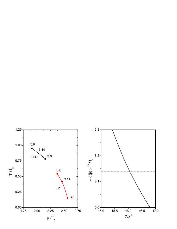
Figure 1: Left: temperature and chemical potential for the TCP and LP, in units of $f_{\pi}$, for different values of the ratio $-(\langle\bar{q}q\rangle^{\rm ch})^{1/3}/f_{\pi}^{\rm ch}$. Right: relation between this ratio and the dimensionless parameter $\bar{G}=G\,\Lambda^{2}$. The dashed line corresponds to the phenomenologically preferred value $-(\langle\bar{q}q\rangle^{\rm ch})^{1/3}/f_{\pi}^{\rm ch}\simeq 3.14$.

A somewhat better understanding of the results can be achieved by taking into account approximate analytical expressions for the GL coefficients. In fact, through the methods discussed in Appendix A of Ref. GomezDumm:2004sr we obtain the relations

$$\alpha_{2} = \frac{1}{G}+\frac{N_{c}}{\pi^{2}}\left[\frac{\pi^{2}}{3}\,T^{2}+\mu^{2}-\int_{0}^{\infty}dp\ p\;g^{2}(p^{2})\right]$$

$$\alpha_{4} = -\frac{N_{c}}{\pi^{2}}\left[4g^{\prime}(0)\left(\frac{\pi^{2}}{3}\,T^{2}+\mu^{2}\right)+\frac{1}{2}+\log{2}-\int_{0}^{\infty}dp\ \frac{g^{4}(p^{2})-n_{+}(p)-n_{-}(p)}{p}\right]$$

$$\alpha_{4b} = -\frac{N_{c}}{\pi^{2}}\left[\ g^{\prime}(0)\left(\frac{\pi^{2}}{3}\,T^{2}+\mu^{2}\right)-\frac{2}{3}\left[g^{\prime}(0)^{2}+g^{\prime\prime}(0)\right]\;\left(\frac{7\pi^{4}}{30}\,T^{4}+\pi^{2}\,T^{2}\,\mu^{2}+\frac{1}{2}\mu^{4}\right)+\right.$$ (14)

$$\qquad\qquad\left.\frac{3}{8}+\log{2}-\int_{0}^{\infty}dp\ \frac{g^{2}(p^{2})-n_{+}(p)-n_{-}(p)}{p}\ \right]\ .$$

The above expression for $\alpha_{4b}$ has not, to our knowledge, been reported before, while those for $\alpha_{2}$ and $\alpha_{4}$ have been already given (using a different notation) in Ref. GomezDumm:2004sr . One can check that in the region of interest these relations provide a very good approximation (in general, below the percent level) to the results arising from the numerical evaluation of the Matsubara sums. In order to determine the relative positions between the TCP and the LP, it is interesting to calculate the coefficient $\alpha_{4b}$ at the TCP, i.e. where $\alpha_{2}=\alpha_{4}=0$. We obtain

$${\alpha_{4b}}^{\rm\tiny{(TCP)}} = \frac{N_{c}}{\pi^{2}}\left\{\pi^{2}\,g^{\prime}(0)\,T_{c}^{2}+\frac{\pi^{4}}{9}\left[g^{\prime}(0)^{2}+g^{\prime\prime}(0)\right]\left[\frac{7}{5}\,T^{4}+2\,T^{2}(T_{c}^{2}-T^{2})+\frac{1}{3}\,(T_{c}^{2}-T^{2})^{2}\right]+\right.$$ (15)

$$\left.\frac{1}{8}-4\int_{0}^{\infty}dp\ p\,\log p\;[1-2g^{2}(p^{2})]\;g(p^{2})\,g^{\prime}(p^{2})\ \right\}\ ,$$

where $T_{c}$ stands for the (second order) chiral phase transition temperature at $\mu=0$. From the GL expansion it is easy to see that the condition $\alpha_{4b}^{\rm\tiny{(TCP)}}>0$ $(<0)$ implies that the LP is located at lower (higher) temperature and higher (lower) chemical potential than those of the TCP. In the particular case of the Gaussian form factor Eq. (15) reduces to

$$\alpha_{4b}^{\tiny\rm(TCP)} = N_{c}\left\{-\,t_{c}^{2}+\frac{1+4\,\log 2}{8\pi^{2}}+\frac{\pi^{2}}{9}\left[\frac{14}{5}\,t^{4}+4\,t^{2}(t_{c}^{2}-t^{2})+\frac{2}{3}\,(t_{c}^{2}-t^{2})^{2}\right]\right\}\ ,$$ (16)

where we have defined $t=T/\Lambda$, $t_{c}=T_{c}/\Lambda$. It can be seen that in this case one can get $\alpha_{4b}^{\rm\tiny{(TCP)}}<0$ only if the dimensionless constant $\bar{G}$ satisfies

$$\bar{G}\;>\;\frac{4\pi^{2}}{N_{c}[\sqrt{6(13-2\log 2)}-8]}\;\simeq\;37.9\ ,$$ (17)

which is far from the phenomenologically accepted range (see lower right panel in Fig. 1).

For definiteness we have discussed so far the particular case of the Gaussian nonlocal form factor in Eq. (13). In order to get an insight of whether the results can be extended to other form factor shapes we have also considered the Lorentzian functions

$$g=\frac{1}{1+(p^{2}/\Lambda^{2})^{n}}\ ,$$ (18)

with $n\geq 2$. For $n=2$, which corresponds to a rather “soft” ultraviolet behavior, the situation concerning the relative positions of the TCP and LP is found to be quite similar to that of the Gaussian form factor. If $n$ is increased, both the TCP and LP tend to be located at lower temperatures, and eventually the LP disappears. In all phenomenologically acceptable cases the TCP is found to be located at a higher temperature and a lower chemical potential than those of the LP. It is also worth mentioning that Eqs. (7) are also valid for “instantaneous” form factors, i.e. those that only depend on space variables, ${\cal G}(|\vec{x}|)$. In general these form factors lead to rather large values of the chiral condensate Grigorian:2006qe . Numerical solutions of Eqs. (11) and (12) allow to find the corresponding locations of the TCP and LP, which are qualitatively similar to those obtained for the covariant form factors.

In conclusion, we have analyzed the relation between the positions of the tricritical point (TCP) and the Landau point (LP) in the framework of the simplest version of nonlocal chiral quark models using the generalized Ginzburg-Landau approach. We have found that for all the phenomenologically acceptable parametrizations considered the TCP is located at a higher temperature and a lower chemical potential in comparison with the LP. Consequently, these models seem to favor a scenario in which the onset of the first order transition between homogeneous phases is not covered by an inhomogeneous, energetically favored phase. This differs from what happens in the local NJL model, where the TCP and LP are predicted to coincide Nickel:2009ke , or in quark-meson models with vacuum fluctuations, where the relative position of these points depends on the model parametrization Carignano:2014jla . The location of the TCP and LP has also been investigated numerically in a recent study based on the Dyson-Schwinger approach Muller:2013tya . Although the corresponding result seems to agree with that of the local NJL model, we should keep in mind that a precise numerical determination of the positions of the TCP and LP is in general a quite difficult task.

Several extensions of our work deserve further investigations. For example, it would be important to incorporate isoscalar vector meson interactions, to consider the coupling to the Polyakov loop and to analyze the effect of wave function renormalization. Moreover, the actual determination of the size of inhomogeneous phases in the $(T,\mu)$ plane in the context of nonlocal models should be feasible, at least for simple inhomogeneous configurations. We expect to report on these issues in forthcoming publications.

This work has been partially funded by CONICET (Argentina) under grants PIP 00682 and PIP 00449, and by ANPCyT (Argentina) under grant PICT11-03-00113.

References

- (1) For a recent review see M. Buballa and S. Carignano, Prog. Part. Nucl. Phys. 81 (2015) 39.
- (2) D. Nickel, Phys. Rev. Lett. 103 (2009) 072301; Phys. Rev. D 80 (2009) 074025.
- (3) U. Vogl and W. Weise, Prog. Part. Nucl. Phys. 27 (1991) 195; S. P. Klevansky, Rev. Mod. Phys. 64 (1992) 649; T. Hatsuda and T. Kunihiro, Phys. Rept. 247 (1994) 221.
- (4) S. Carignano, M. Buballa and B. J. Schaefer, Phys. Rev. D 90 (2014) 014033.
- (5) T. Schafer and E. V. Shuryak, Rev. Mod. Phys. 70 (1998) 323.
- (6) C. D. Roberts and A. G. Williams, Prog. Part. Nucl. Phys. 33 (1994) 477; C. D. Roberts and S. M. Schmidt, Prog. Part. Nucl. Phys. 45 (2000) S1.
- (7) S. Noguera and N. N. Scoccola, Phys. Rev. D 78 (2008) 114002.
- (8) P. O. Bowman, U. M. Heller, and A. G. Williams, Phys. Rev. D 66 (2002) 014505; P. O. Bowman, U. M. Heller, D. B. Leinweber and A. G. Williams, Nucl. Phys. Proc. Suppl. 119 (2003) 323.
- (9) M. B. Parappilly, P. O. Bowman, U. M. Heller, D. B. Leinweber, A. G. Williams and J. B. Zhang, Phys. Rev. D 73 (2006) 054504.
- (10) S. Furui and H. Nakajima, Phys. Rev. D 73 (2006) 074503.
- (11) G. Ripka, Quarks bound by chiral fields (Oxford University Press, Oxford, 1997).
- (12) R.D. Bowler and M.C. Birse, Nucl. Phys. A 582 (1995) 655; R.S. Plant and M.C. Birse, Nucl. Phys. A 628 (1998) 60.
- (13) S. M. Schmidt, D. Blaschke and Y. L. Kalinovsky, Phys. Rev. C 50 (1994) 435.
- (14) B. Golli, W. Broniowski and G. Ripka, Phys. Lett. B 437 (1998) 24; W. Broniowski, B. Golli and G. Ripka, Nucl. Phys. A 703 (2002) 667.
- (15) D. Gomez Dumm and N.N. Scoccola, Phys. Rev. D 65 (2002) 074021.
- (16) A. Scarpettini, D. Gomez Dumm and N.N. Scoccola, Phys. Rev. D 69 (2004) 114018.
- (17) D. Gomez Dumm and N. N. Scoccola, Phys. Rev. C 72 (2005) 014909.
- (18) D. Gomez Dumm, A. G. Grunfeld and N.N. Scoccola, Phys. Rev. D 74 (2006) 054026.
- (19) T. Hell, S. Roessner, M. Cristoforetti and W. Weise, Phys. Rev. D 79 (2009) 014022.
- (20) G. A. Contrera, D. Gomez Dumm and N. N. Scoccola, Phys. Rev. D 81 (2010) 054005.
- (21) T. Hell, S. Rossner, M. Cristoforetti and W. Weise, Phys. Rev. D 81 (2010) 074034.
- (22) G. A. Contrera, M. Orsaria and N. N. Scoccola, Phys. Rev. D 82 (2010) 054026.
- (23) D. Gomez Dumm, S. Noguera and N.N. Scoccola, Phys. Lett. B 698 (2011) 236; Phys. Rev. D 86 (2012) 074020.
- (24) V. Pagura, D. Gomez Dumm and N. N. Scoccola, Phys. Lett. B 707 (2012) 76.
- (25) J. P. Carlomagno, D. Gómez Dumm and N. N. Scoccola, Phys. Rev. D 88 (2013) 074034.
- (26) H. Abuki, D. Ishibashi and K. Suzuki, Phys. Rev. D 85 (2012) 074002.
- (27) Y. Iwata, H. Abuki and K. Suzuki, arXiv:1206.2870 [hep-ph].
- (28) S. Aoki, Y. Aoki, C. Bernard, T. Blum, G. Colangelo, M. Della Morte, S. Dürr and A. X. El Khadra et al., Eur. Phys. J. C 74 (2014) 2890.
- (29) H. Grigorian, Phys. Part. Nucl. Lett. 4 (2007) 223.
- (30) D. Müller, M. Buballa and J. Wambach, Phys. Lett. B 727 (2013) 240.