Single Spin Asymmetry in Electroproduction of $J/\psi$ and QCD-evolved TMD’s

Abstract

We estimate Sivers asymmetry in low virtuality photoproduction of $J/\psi$ using color evaporation model and taking into account $Q^{2}$- evolution of transverse momentum dependent PDF’s and Sivers function. There is a substantial reduction in asymmetry as compared to our previous analysis wherein the $Q^{2}$-dependance came only from DGLAP evolution of collinear part of TMDs. The estimates of asymmetry are comparable to our earlier estimates in which we had used analytical solution of only an approximated form of the evolution equations. We have also estimated asymmetry using the latest parametrization by Echevarria et al. which are based on an evolution kernel in which the perturbative part is resummed to NLL accuracy.

PACS numbers:13.88+e, 13.60.-r, 14.40.Lb, 29.25.Pj.

1 Introduction

The issue of quarkonium production mechanism is an open question as none of theoretical models which are used to describe the non-perturbative transformation of the $Q{\bar{Q}}$ pair into quarkonium i.e. the Color Singlet Modeal (CSM)[1][3], Color Evaporation Model (CEM)[4] and Non-Relativistic Quantum Chromodynamics (NRQCD)[5], is able to explain satisfactorily all the data on both production cross section and polarization measurements. Thus, independent tests other than polarization measurements are needed to compare the different production mechanisms. One such possible test is transverse single spin asymmetry (SSA) in charmonium production[6, 7, 8] since the asymmetry in heavy quarkonium production is very sensitive to the production mechanism[9].

One of the theoretical approaches that has been used to explain these asymmetries in Semi-Inclusive Deep Inelastic Scattering (SIDIS) and Drell Yan (DY) processes is based on a transverse momentum dependent factorization scheme[10, 11] which involves transverse momentum dependent parton densities and fragmentation functions collectively referred to as TMD’s. One such TMD of great interest is Sivers function which gives the probability of finding an unpolarized parton inside a transversly polarized nucleon.

In an earlier work, we proposed that transverse SSA in charmonium production can be used to study Sivers effect[6]. We presented first estimates of SSA in photoproduction (i.e. low virtuality electroproduction) of charmonium in scattering of electrons off transversely polarized protons using CEM. In the process that we considered, at LO, there is contribution only from a single partonic subprocess and hence, it can be used as a clean probe of gluon Sivers function. Subsequently, we improved our estimates taking into account TMD evolution of TMD PDF’s and the Sivers function[12]. In present work, we present further improved estimates calculated using the latest fits to TMD PDF’s given by Echevarria et al.[13] and compare them with our earlier estimates.

2 Transverse Single Spin Asymmetry in $e+p^{\uparrow}\rightarrow J/\psi+X$

We will use a generalization of CEM for our estimates of asymmetry in photoproduction (low virtuality electroproduction) of $J/\psi$ by taking into account the transverse momentum dependence of the WW function and the gluon distribution function [6]

$$\sigma^{e+p^{\uparrow}\rightarrow e+J/\psi+X}=\int_{4m_{c}^{2}}^{4m_{D}^{2}}dM_{c\bar{c}}^{2}dx_{\gamma}dx_{g}[d^{2}{\bf k}_{\perp\gamma}d^{2}{\bf k}_{\perp g}]f_{g/p^{\uparrow}}(x_{g},{\bf k}_{\perp g})$$

$$\times f_{\gamma/e}(x_{\gamma},{\bf k}_{\perp\gamma})\frac{d\hat{\sigma}^{\gamma g\rightarrow c\bar{c}}}{dM_{c\bar{c}}^{2}}$$ (1)

where $f_{\gamma/e}(y,E)$ is the William Weizsacker function[14] which gives distribution function of the photon in the electron. We assume $k_{\perp}$ dependence of pdf’s to be factorized in gaussian form [15]

$$f(x,k_{\perp})=f(x)\frac{1}{\pi\langle k^{2}_{\perp}\rangle}e^{-k^{2}_{\perp}/\langle{k^{2}_{\perp}\rangle}}$$ (2)

with $\langle k^{2}_{\perp}\rangle=0.25GeV^{2}$. For the ${\bf k}_{\perp}$ dependent WW function also, we use a Gaussian form. Expression for the numerator of the asymmetry is[6]

$$\frac{d^{4}\sigma^{\uparrow}}{dyd^{2}{\bf q}_{T}}-\frac{d^{4}\sigma^{\downarrow}}{dyd^{2}{\bf q}_{T}}=\frac{1}{2}\int_{4m^{2}_{c}}^{4m^{2}_{D}}[dM^{2}]\int[dx_{\gamma}dx_{g}d^{2}{\bf k}_{\perp\gamma}d^{2}{\bf k}_{\perp g}]\Delta^{N}f_{g/p^{\uparrow}}(x_{g},{\bf k}_{\perp g})$$

$$\times f_{\gamma/e}(x_{\gamma},{\bf k}_{\perp\gamma})\delta^{4}(p_{g}+p_{\gamma}-q)\>\hat{\sigma}_{0}^{\gamma g\rightarrow c\bar{c}}(M^{2})$$ (3)

where $q=p_{c}+p_{\bar{c}}$ and the ${{\hat{\sigma}}_{0}}^{\gamma g\rightarrow c\bar{c}}(M^{2})$ is the partonic cross section in lowest order (LO).

In Eq.(3), $\Delta^{N}f_{g/p^{\uparrow}}(x,{\bf k}_{\perp})$ is the gluon Sivers function for which we use the following parametrization[16]

$$\Delta^{N}f_{g/p^{\uparrow}}(x,k_{\perp})=2{\mathcal{N}}_{g}(x)\sqrt{2e}\,\frac{{k_{\perp}}}{M_{1}}\,e^{-{{k_{\perp}}^{2}}/{M_{1}^{2}}}f_{g/p}(x)\frac{e^{-k^{2}_{\bot}/\langle{k^{2}_{\bot}\rangle}}}{\pi\langle k^{2}_{\perp}\rangle}({\bf S}\cdot{\hat{\bf p}}\times{\hat{\bf k}}_{\perp})$$ (4)

Here, ${\mathcal{N}}_{g}(x)$ is the x dependent normalization for which we have used ${\mathcal{N}}_{g}(x)=\left({\mathcal{N}}_{u}(x)+{\mathcal{N}}_{d}(x)\right)/2$[17]. Since there is not enough data available to parametrize the gluon Sivers function, we have expressed gluon Sivers function in terms of quark Sivers function. For quark Sivers functions, we use the following normalization

$${\mathcal{N}}_{f}(x)=N_{f}x^{a_{f}}(1-x)^{b_{f}}\frac{(a_{f}+b_{f})^{(a_{f}+b_{f})}}{{a_{f}}^{a_{f}}{b_{f}}^{b_{f}}}$$

where $a_{f},b_{f}$ and $N_{f}$ are best fit parameters.

Taking $sin(\phi_{q}-\phi_{S})$ as a weight, the asymmetry integrated over the azimuthal angle of $J/\psi$ is

$$A_{N}=\frac{\int d\phi_{q}[\int_{4m^{2}_{c}}^{4m^{2}_{D}}[dM^{2}]\int[d^{2}{\bf k}_{\perp g}]\Delta^{N}f_{g/p^{\uparrow}}(x_{g},{\bf k}_{\perp g})f_{\gamma/e}(x_{\gamma},{\bf q}_{T}-{\bf k}_{\perp g})\hat{\sigma}_{0}]sin(\phi_{q}-\phi_{S})}{2\int d\phi_{q}[\int_{4m^{2}_{c}}^{4m^{2}_{D}}[dM^{2}]\int[d^{2}{\bf k}_{\perp g}]f_{g/P}(x_{g},{\bf k}_{\perp g})f_{\gamma/e}(x_{\gamma},{\bf q}_{T}-{\bf k}_{\perp g})\hat{\sigma}_{0}]}$$ (5)

where $\phi_{q}$ and $\phi_{k_{\perp}}$ are the azimuthal angles of the transverse momenta $q_{T}$ and $k_{\perp}$ and $x_{g,\gamma}=\frac{M}{\sqrt{s}}\,e^{\pm y}$.

3 QCD Evolution of TMD PDF’s

Initial phenomenological fits of the Sivers function and other TMD’s used TMDs which do not evolve with the scale of the process[19, 16]. Our initial estimates of Sivers asymmetry were based on these parameters and the TMDs used were evolved using DGLAP evolution wherein only the collinear part evolves and the Gaussian width of the transverse part is assumed to be fixed. In recent years, the TMD factorization has been derived and implemented [11, 20, 21].

A strategy to extract Sivers function from SIDIS data taking into account the TMD $Q^{2}$ evolution was proposed by Anselmino et al.[22]. We have also estimated SSA in electroproduction of $J/\psi$ production based on this strategy [12]. In present work, we compare our earlier estimates with improved estimates obtained using exact solution of evolution equation. In addition, we have also estimated asymmetry using the latest parametrization by Echevarria et al.[13] which are based on an evolution kernel in which the perturbative part is resummed to NLL accuracy.

The energy evolution of a general TMD $F(x,k_{\perp},Q)$ is more naturally described in b-space. The b-space TMD’s evolves with Q according to

$$F(x,b,Q_{f})=F(x,b,Q_{i})R_{pert}(Q_{f},Q_{i},b_{*})R_{NP}(Q_{f},Q_{i},b)$$ (6)

where $R_{pert}$ is the perturbative part of the evolution kernel, $R_{NP}$ is the non-perturbative part and $b_{*}=b/\sqrt{1+(b/b_{\text{max}})^{2}}$. The perturbative part is given by

$$R(Q_{f},Q_{i},b)=\exp\left\{-\int_{Q_{i}}^{Q_{f}}\frac{d\mu}{\mu}\left(A\ln\frac{Q_{f}^{2}}{\mu^{2}}+B\right)\right\}\left(\frac{Q_{f}^{2}}{Q_{i}^{2}}\right)^{-D(b;Q_{i})}$$ (7)

where $\frac{dD}{d\ln\mu}=\Gamma_{\text{cusp}}$ The anomalous dimensions $A$ and $B$ are known up to three loop level[23]. The non-perturbative exponential part contains a Q-dependent factor universal to all TMDs and a factor which gives the gaussian width in $b$-space of the particular TMD

$$R_{NP}=\exp\left\{-b^{2}\left(g_{1}^{\text{TMD}}+\frac{g_{2}}{2}\ln\frac{Q_{f}}{Q_{i}}\right)\right\}$$ (8)

The $b_{*}$ prescription stitches together the perturbative part(which is valid at low $b$) and non-perturbative part(which is valid at large b. $Q^{2}$-dependent TMD’s in momentum space are obtained by Fourier transforming $F(x,b,Q_{f})$.

4 Approximate Analytical versus Exact Solution of TMD Evolution Equations

In the analytical approach of Anselmino et al. [22] , one assumes that the kernel $R(Q,Q_{0},b)$, which drives the $Q^{2}$-evolution of TMD’s, becomes independent of b in large b limit, i.e. as $b\rightarrow\infty$ , $R(Q,Q_{0},b)\rightarrow R(Q,Q_{0})$. $b$ integration can then be performed analytically and $Q^{2}$ dependent PDF’s can be obtained. In our earlier work, we used $Q^{2}$-evolved TMD PDF’s obtained using this ”approximate, analytical” approach. We will now compare these results with estimates obtained using exact solution of TMD evolution equations which can be obtained by solving the TMD evolution equation numerically[22].

Recently, Echevarria et al.[13] have considered solution of TMD evolution equations up to NLL accuracy and have performed a global fitting of all experimental data on the Sivers asymmetry in SIDIS using this formalism. Since the derivative of b-space Sivers function satisfies the same evolution equation as the unpolarized PDF[21], its evolution is given by

$$f^{\prime\perp g}_{1T}(x,b;Q_{f})= \frac{M_{p}b}{2}T_{g,F}(x,x,Q_{i})\exp\left\{-\int_{Q_{i}}^{Q_{f}}\frac{d\mu}{\mu}\left(A\ln\frac{Q^{2}}{\mu^{2}}+B\right)\right\}\left(\frac{Q_{f}^{2}}{Q_{i}^{2}}\right)^{-D(b^{*};Q_{i})}$$

$$\times \exp\left\{-b^{2}\left(g_{1}^{\text{sivers}}+\frac{g_{2}}{2}\ln\frac{Q_{f}}{Q_{i}}\right)\right\}$$ (9)

where $T_{q,F}(x,x,Q)$ is the twist three Qui-Sterman quark gluon correlation function which is related to the first $k_{\perp}$ moment of quark Sivers function[24] and can be expressed in terms of the unpolarized collinear PDFs [25, 13].

$$T_{q,F}(x,x,Q)=\mathcal{N}_{q}(x)f_{q/P}(x,Q)$$ (10)

The expansion coefficients with the appropriate gluon anomalous dimensions at NLL, $A^{(1)},A^{(2)},B^{(1)}$ and $D^{(1)},$ are known[13]. Choosing the initial scale $Q_{i}=c/b$, the $D$ term vanishes at NLL. Taking Fourier transform of Eq. (9), one gets $f^{\perp g}_{1T}(x,k_{\perp};Q_{f})$ which is related to Sivers function through

$$\Delta^{N}f_{g/p^{\uparrow}}(x_{g},\mbox{\boldmath$k$}_{\perp g},Q)=-2\frac{k_{\perp g}}{M_{p}}f^{\perp g}_{1T}(x_{g},k_{\perp g};Q)\cos\phi_{k_{\perp}}$$ (11)

5 Numerical Estimates of Asymmetry using analytical and exact formalisms

We will now present our estimates of SSA in photoproduction of $J/\psi$ for JLAB, HERMES, COMPASS and eRHIC energies. A detailed discussion of results can be found in Ref. Godbole:2014tha. Figs. 1-5 show the y and $k_{T}$ distribution for different experiments with parameterizations TMD Exact-1, TMD Exact -2 and TMD a given in Table 1. TMD-e1 parameter set, extracted at $Q_{0}=1.0\text{ GeV}$, is for the exact solution of TMD evolution equations extracted in Ref. Anselmino:2012aa. TMD-a is the parameter set extracted using an analytical approximated form of evolution equations given in Ref. Anselmino:2012aa. For estimates using NLL kernel we have used the most recent parameters by Echevarria et al.[13] obtained by performing a global fit of all experimental data on Sivers asymmetry in SIDIS from HERMES, COMPASS and JLAb. We call this set TMD-e2. This set was fitted at $Q_{0}=\sqrt{2.4}\text{ GeV}$. Fig. 6 shows a comparison of asymmetries at all energies.

6 Summary

We have compared estimates of SSA in electroproduction of $J/\psi$ using TMD’s evolved via DGLAP evolution and TMD evolution schemes. For the latter, we have chosen three different parameter sets fitted using an approximate analytical solution, an exact solution at LL and an exact solution at NLL. We find that the estimates given by TMD evolved PDF’s and Sivers function are all comparable but substantially small as compared to estimates calculated using DGLAP evolved TMD’s.

TMD-e1	TMD-a	TMD-e2
$N_{u}=0.77,N_{d}=-1.00$	$N_{u}=0.75,N_{d}=-1.00$	$N_{u}=0.106,N_{d}=-0.163$
$a_{u}=0.68,a_{d}=1.11$	$a_{u}=0.82,a_{d}=1.36$	$a_{u}=1.051,a_{d}=1.552$
$b_{u}=b_{d}=3.1,$	$b_{u}=b_{d}=4.0,$	$b_{u}=b_{d}=4.857$,
$M_{1}^{2}=0.40\text{GeV}^{2}$	$M_{1}^{2}=0.34\text{GeV}^{2}$	$\langle k^{2}_{s\perp}\rangle=0.282\text{ GeV}^{2}$
$\langle k^{2}_{\perp}\rangle=0.25\text{GeV}^{2}$	$\langle k^{2}_{\perp}\rangle=0.25\text{GeV}^{2}$	$\langle k^{2}_{\perp}\rangle=0.38\text{GeV}^{2}$
$b_{max}=0.5GeV^{-1}$	$b_{max}=0.5GeV^{-1}$	$b_{max}=1.5GeV^{-1}$
$g_{2}=0.68\text{ GeV}^{2}$	$g_{2}=0.68\text{ GeV}^{2}$	$g_{2}=0.16\text{ GeV}^{2}$

Table 1: Parameter sets

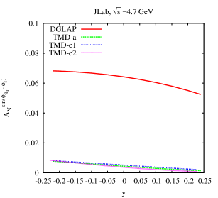
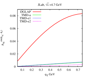
Figure 1: The Sivers asymmetry $A_{N}^{\sin({\phi}_{q_{T}}-\phi_{S})}$ for $e+p^{\uparrow}\rightarrow e+J/\psi+X$ at JLab energy ($\sqrt{s}=4.7$ GeV), as a function of $y$ (left panel) and $q_{T}$ (right panel). The integration ranges are $(0\leq q_{T}\leq 1)$ GeV and $(-0.25\leq y\leq 0.25)$.

.

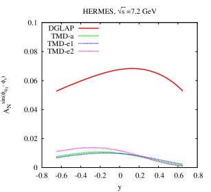
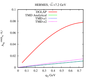
Figure 2: HERMES energy ($\sqrt{s}=7.2$ GeV), Asymmetry as a function of $y$ (left panel) and $q_{T}$ (right panel). The integration ranges are $(0\leq q_{T}\leq 1)$ GeV and $(-0.6\leq y\leq 0.6)$.

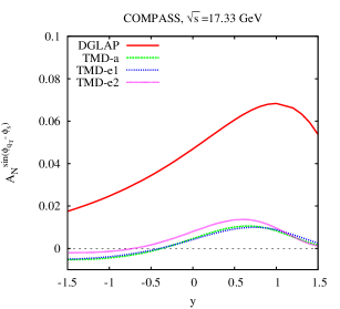
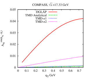
Figure 3: COMPASS energy ($\sqrt{s}=17.33$ GeV),Asymmetry as a function of $y$ (left panel) and $q_{T}$ (right panel). The integration ranges are $(0\leq q_{T}\leq 1)$ GeV and $(-1.5\leq y\leq 1.5)$.

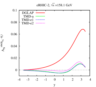
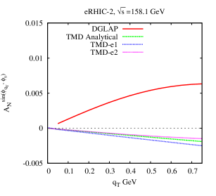
Figure 4: eRHIC energy ($\sqrt{s}=158.1$ GeV),Asymmetry as a function of $y$ (left panel) and $q_{T}$ (right panel). . The integration ranges are $(0\leq q_{T}\leq 1)$ GeV and $(-3.7\leq y\leq 3.7)$.

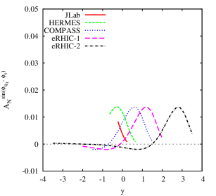
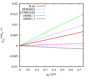
Figure 5: Left panel: Plot of the Sivers asymmetries in the $y$ distribution obtained in all c.o.m energies using the TMD-e2 fit . This plot shows the drift of the asymmetry peak towards higher values of rapidity $y$. Right panel: Plot of the Sivers Asymmetries in the $q_{T}$ distribution

References

• [1] M.B. Einhorn and S.D. Ellis Phys. Rev. D 12, 2007 (1975)
• [2] J.P. Lansberg, Eur. Phys. J. C 61, 693 (2009)
• [3] J.P.Lansberg, Phys. Lett. B 695, 149 (2010)
• [4] H. Fritsch, Phys. Lett. B 67, 217 (1977).
• [5] G. T. Bodwin, E. Braaten and G. P. Lepage, Phys. Rev. D 51, 1125 (1995) [Erratum-ibid. D 55, 5853 (1997)] [hep-ph/9407339].
• [6] R. M. Godbole, A. Misra, A. Mukherjee and V. S. Rawoot, Phys. Rev. D 85, 094013 (2012) [arXiv:1201.1066 [hep-ph]].
• [7] S.J. Brodsky, D.S. Hwang, I. Schmidt, Phys. Lett. B530, 99(2002)
• [8] S.J. Brodsky, D.S. Hwang, I. Schmidt, Nucl. Phys. B 642, 344(2002)
• [9] F. Yuan, Phys. Rev. D 78, 014024 (2008) [arXiv:0801.4357 [hep-ph]].
• [10] J. C. Collins and D. E. Soper, Nucl. Phys. B 193, 381 (1981) [Erratum-ibid. B 213, 545 (1983)] [Nucl. Phys. B 213, 545 (1983)]; X. -d. Ji, J. -p. Ma and F. Yuan, Phys. Rev. D 71, 034005 (2005) [hep-ph/0404183].
• [11] J. C. Collins, Foundations of Perturbative QCD, Cambridge Monographs on Particle Physics, Nuclear Physics and Cosmology, No. 32, Cambridge University Press, Cambridge, 2011.
• [12] R. M. Godbole, A. Misra, A. Mukherjee and V. S. Rawoot, Phys. Rev. D 88, no. 1, 014029 (2013) [arXiv:1304.2584 [hep-ph]].
• [13] M. G. Echevarria, A. Idilbi, Z. -B. Kang and I. Vitev, Phys. Rev. D 89, 074013 (2014) [arXiv:1401.5078 [hep-ph]].
• [14] B.A Kniehl Phys. Lett.B 254, 267(1991)
• [15] M. Anselmino, M. Boglione, U. D’Alesio, A. Kotzinian, F. Murgia and A. Prokudin, Phys. Rev. D 72, 094007 (2005) [Erratum-ibid. D 72, 099903 (2005)] [hep-ph/0507181].
• [16] M. Anselmino et al., Eur. Phys. J. A 39, 89 (2009)
• [17] D. Boer and W. Vogelsang, Phys. Rev. D 69, 094025 (2004) [hep-ph/0312320].
• [18] M. Anselmino, M. Boglione, U. D’Alesio, S. Melis, F. Murgia and A. Prokudin, Phys. Rev. D 79, 054010 (2009) [arXiv:0901.3078 [hep-ph]].
• [19] J.C. Collins et al., Phys. Rev. D 73, 014021(2006)
• [20] S. M. Aybat and T. C. Rogers, Phys. Rev. D 83, 114042 (2011) [arXiv:1101.5057 [hep-ph]].
• [21] S. M. Aybat, J. C. Collins, J. -W. Qiu and T. C. Rogers, arXiv:1110.6428 [hep-ph].
• [22] M. Anselmino, M. Boglione and S. Melis, Phys. Rev. D 86, 014028 (2012) [arXiv:1204.1239 [hep-ph]].
• [23] A. Idilbi, X. -d. Ji and F. Yuan, Nucl. Phys. B 753, 42 (2006) [hep-ph/0605068].
• [24] Z. -B. Kang, B. -W. Xiao and F. Yuan, Phys. Rev. Lett.  107, 152002 (2011) [arXiv:1106.0266 [hep-ph]].
• [25] C. Kouvaris, J. -W. Qiu, W. Vogelsang and F. Yuan, Phys. Rev. D 74, 114013 (2006) [hep-ph/0609238].
• [26] R. M. Godbole, A. Kaushik, A. Misra and V. S. Rawoot, arXiv:1405.3560 [hep-ph].