Following the evolution of glassy states under external perturbations:
compression and shear-strain

Abstract

We consider the adiabatic evolution of glassy states under external perturbations. Although the formalism we use is very general, we focus here on infinite-dimensional hard spheres where an exact analysis is possible. We consider perturbations of the boundary, i.e. compression or (volume preserving) shear-strain, and we compute the response of glassy states to such perturbations: pressure and shear-stress. We find that both quantities overshoot before the glass state becomes unstable at a spinodal point where it melts into a liquid (or yields). We also estimate the yield stress of the glass. Finally, we study the stability of the glass basins towards breaking into sub-basins, corresponding to a Gardner transition. We find that close to the dynamical transition, glasses undergo a Gardner transition after an infinitesimal perturbation.

Introduction –

Glasses are long lived metastable states of matter, in which particles are confined around an amorphous structure Cavagna (2009); Dyre (2006). For a given sample of a material, the glass state is not unique: depending on the preparation protocol, the material can be trapped in different glasses, each displaying different thermodynamic properties. For example, the specific volume of a glass prepared by cooling a liquid depends strongly on the cooling rate Cavagna (2009); Dyre (2006). Other procedures, such as vapor deposition, produce very stable glasses, with higher density than those obtained by simple cooling Swallen et al. (2007); Singh et al. (2013). When heated up, glasses show hysteresis: their energy (specific volume) remains below the liquid one, until a “spinodal” point is reached, at which they melt into the liquid (see e.g. (Dyre, 2006, Fig.1) and (Singh et al., 2013, Fig.2)).

The behavior of glasses under shear-strain also shows similarly complex phenomena. Suppose to prepare a glass by cooling a liquid at a given rate until some low temperature $T$ is reached. After cooling, a strain $\gamma$ is applied and the stress $\sigma$ is recorded. At small $\gamma$, an elastic (linear) regime where $\sigma\sim\mu\gamma$ is found. At larger $\gamma$, the stress reaches a maximum and then decreases until an instability is reached, where the glass yields and starts to flow (see e.g. (Rodney et al., 2011, Fig.3c) and (Koumakis et al., 2012, Fig.2)). The amplitude of the shear modulus $\mu$ and of the stress overshoot increase when the cooling rate is decreased, and more stable glasses are reached.

Computing these observables theoretically is a difficult challenge, because glassy states are always prepared through non-equilibrium dynamical protocols. First-principle dynamical theories such as Mode-Coupling Theory (MCT) Götze (2009) are successful in describing properties of supercooled liquids close to the glass state (including the stress overshoot Brader et al. (2009)), but they fail to describe glasses at low temperatures and high pressures Ikeda and Berthier (2013). The dynamical facilitation picture can successfully describe calorimetric properties of glasses Keys et al. (2013), but for the moment it does not allow one to perform first-principles calculations starting from the microscopic interaction potential. To bypass the difficulty of describing all the dynamical details of glass formation, one can exploit a standard idea in statistical mechanics, namely that metastable states are described by a restricted equilibrium thermodynamics for times much shorter than their lifetimes Penrose and Lebowitz (1971); Langer (1974). Within schematic models of glasses, this construction was proposed by several authors Kirkpatrick and Wolynes (1987); Kirkpatrick and Thirumalai (1989); Monasson (1995); Franz and Parisi (1995) and was formalised through the Franz-Parisi free energy Franz and Parisi (1995) and the “state following” formalism Barrat et al. (1997); Zdeborová and Krzakala (2010); Krzakala and Zdeborová (2013).

In this paper we apply the state following construction Franz and Parisi (1995); Barrat et al. (1997); Zdeborová and Krzakala (2010); Krzakala and Zdeborová (2013) to a realistic model of glass former, made by identical particles interacting in the continuum. For simplicity, we choose here hard spheres in spatial dimension $d\rightarrow\infty$, where the method is exact because metastable states have infinite lifetime Kirkpatrick and Wolynes (1987); Parisi and Zamponi (2010); Charbonneau et al. (2014a). We show that all the properties of glasses mentioned above are predicted by this framework, including the cooling rate dependence of the specific volume (or the pressure) Dyre (2006); Cavagna (2009), the hysteresis observed upon heating glasses Dyre (2006); Swallen et al. (2007); Singh et al. (2013), the behavior of the shear modulus and the stress overshoot Rodney et al. (2011); Koumakis et al. (2012). Following Mezard and Parisi (2012); Parisi and Zamponi (2010), our method can be generalized (under standard liquid theory approximations) to experimentally relevant systems in $d=2,3$ with different interaction potentials, to obtain precise quantitative predictions, as we discuss in the conclusions.

Constrained thermodynamics –

The “state following” formalism is designed to describe glass formation during slow cooling of a liquid Krzakala and Zdeborová (2013). Approaching the glass transition, the equilibrium dynamics of the liquid happens on two well separated time scales Dyre (2006); Cavagna (2009). On a $T$-independent fast scale $\tau_{\rm vib}$ particles essentially vibrate in the cages formed by their neighbors. On the slow $\alpha$-relaxation scale $\tau_{\alpha}(T)$, that increases fast approaching the glass transition, cooperative processes change the structure of the material. When $\tau_{\alpha}(T)\gg\tau_{\rm vib}$, the system vibrates for a long time around a locally stable configuration of the particles (a glass), and then on a time scale $\tau_{\alpha}(T)$ transforms in another equivalent glass. Hence, $\tau_{\alpha}(T)$ is the lifetime of metastable glasses. The liquid reaches equilibrium if enough different glass states are visited, hence the experimental time scale (e.g. the cooling rate) should be $\tau_{\rm exp}\gg\tau_{\alpha}(T)$. For given $\tau_{\rm exp}$, the glass transition temperature $T_{g}$ is therefore defined by $\tau_{\rm exp}=\tau_{\alpha}(T_{g})$ Dyre (2006); Cavagna (2009). For $T<T_{g}$ the system is confined into a given glass with lifetime $\tau_{\alpha}(T)\gg\tau_{\rm exp}$, which can thus be considered an infinitely-long lived metastable state. Although the system is strictly speaking out of equilibrium in this regime, the slow relaxation is effectively frozen and the material is confined in a thermodynamic equilibrium state restricted to a given glass. In fact, if cooling stops at some $T<T_{g}$, thermodynamic quantities quickly reach time-independent values, that satisfy equilibrium thermodynamic relations. Still, the “thermodynamic” state depends on preparation history, and most crucially on the temperature $T_{g}$ at which the liquid fell out of equilibrium. Note that aging effects can be neglected here because they happen, for $T<T_{g}$, on time scales $\tau_{\rm aging}\gg\tau_{\alpha}(T_{g})\sim\tau_{\rm exp}$.

This observation suggests how to describe the thermodynamic properties of glasses prepared by slow cooling Franz and Parisi (1995); Barrat et al. (1997); Zdeborová and Krzakala (2010); Krzakala and Zdeborová (2013). Consider $N$ interacting classical particles, described by coordinates $X=\{x_{i}\}_{i=1,\cdots,N}$ and potential energy $V(X)$. During a cooling process with time scale $\tau_{\rm exp}$, the system remains equilibrated provided $T\geq T_{g}$. Define $R=\{r_{i}\}$ the last configuration visited by the material before falling out of equilibrium; its probability distribution is the equilibrium one at $T_{g}$, $P(R)=\exp[-V(R)/T_{g}]/Z(T_{g})$ (here $k_{B}=1$). For $T<T_{g}$, the lifetime of glasses becomes effectively infinite : the material visits configurations $X$ confined in the glass selected by $R$. This constraint is implemented Franz and Parisi (1995); Barrat et al. (1997) by imposing that the mean square displacement between $X$ and $R$, $\Delta(X,R)=(d/N)\sum_{i=1}^{N}(x_{i}-r_{i})^{2}$, be smaller than a prescribed value $\Delta^{\rm r}$. The evolution of this glass is followed by changing its temperature $T$ or applying some perturbation $\gamma$ that changes the potential to $V_{\gamma}$. The free energy of the glass selected by $R$ is therefore

$$F_{g}[T,\gamma;R]=-T\log\int dXe^{-V_{\gamma}[X]/T}\theta[\Delta^{\rm r}-\Delta(X,R)]\ .$$

$\theta(x)$ is the Heaviside function. Computing $F_{g}[T,\gamma;R]$ is a formidably difficult task, because the constraint $\Delta(X,R)\leq\Delta^{\rm r}$ explicitly breaks translational invariance and prevents one from using standard statistical mechanics methods. One can simplify the problem by computing the average free energy of all glasses that are sampled by liquid configurations at $T_{g}$, under the assumption that these glasses have similar thermodynamic properties. We obtain

$$F_{g}[T,\gamma]=\overline{F_{g}[T,\gamma;R]}=\int dR\frac{e^{-V(R)/T_{g}}}{Z(T_{g})}F_{g}[T,\gamma;R]\ .$$

This average can be computed using the replica trick Franz and Parisi (1995), and here we use the simplest replica symmetric (RS) scheme Franz and Parisi (1995); Barrat et al. (1997); Zdeborová and Krzakala (2010). The parameter $\Delta^{\rm r}$ is determined by minimizing the free energy, see the Appendix.

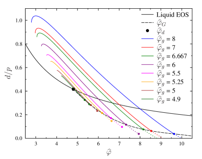
Figure 1: Following glasses in (de)compression. Inverse reduced pressure $d/p$ is plotted versus packing fraction $\widehat{\varphi}=2^{d}\varphi/d$. Both quantities are scaled to have a finite limit for $d\rightarrow\infty$. The liquid EOS is $d/p=2/\widehat{\varphi}$. The dynamical transition $\widehat{\varphi}_{\rm d}$ is marked by a black dot. For $\widehat{\varphi}_{g}>\widehat{\varphi}_{\rm d}$, the liquid is a collection of glasses. The glassy EOS are reported as full colored lines, that intersect the liquid EOS at $\widehat{\varphi}_{g}$. Upon compression, a glass prepared at $\widehat{\varphi}_{g}$ undergoes a Gardner transition at $\widehat{\varphi}_{G}(\widehat{\varphi}_{g})$ (full symbols and long-dashed black line). Beyond $\widehat{\varphi}_{G}$ our computation is not correct: glass EOS are reported as dashed lines. For low $\widehat{\varphi}_{g}$ they end at an unphysical spinodal point (open symbol). Upon decompression, the glass pressure falls below the liquid one, until it reaches a minimum, and then grows again until a physical spinodal point at which the glass melts into the liquid.

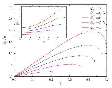
Figure 2: Following glassy states prepared at $\widehat{\varphi}_{g}$ upon applying a shear-strain $\gamma$. Shear-stress $\sigma$ (main panel) and reduced pressure $p$ (inset) as a function of strain for different $\widehat{\varphi}_{g}$. Same styles as Fig. 1. Upon increasing shear-strain, the states undergo a Gardner transition at $\gamma_{G}(\widehat{\varphi}_{g})$. For $\gamma>\gamma_{G}$ our RS computation is unstable but it predicts a stress overshoot followed by a spinodal point.

This computation was done for spin glasses in Franz and Parisi (1995); Barrat et al. (1997); Zdeborová and Krzakala (2010); Krzakala and Zdeborová (2013); Franz et al. and describes perfectly the properties of glasses obtained by slow cooling Krzakala and Zdeborová (2013). Here we consider a realistic glass-former: a hard sphere system for $d\rightarrow\infty$. Technically, the computation uses the methods of Charbonneau et al. (2014a) in the more complicated state following setting. Because the details are not particularly instructive, we report them in the Appendix, where we also discuss the conceptual differences with respect to previous works Parisi and Zamponi (2010); Charbonneau et al. (2014a).

Results: compression –

As a first application of the method, we consider preparing glasses by slow compression, which is equivalent, for hard spheres, to slow cooling Parisi and Zamponi (2010). Note that for hard spheres temperature can be eliminated by appropriately rescaling physical quantities. The system is prepared at low density $\rho$, particle volume $V_{s}$ is slowly increased (equivalently, container volume is decreased), and pressure $P$ is monitored. In Fig. 1 we plot the reduced pressure $p=\beta P/\rho$, with $\beta=1/T$, versus the packing fraction $\varphi=\rho V_{s}$. At equilibrium, the system follows the liquid equation of state (EOS). Above the so-called dynamical transition (or MCT transition) density $\varphi_{\rm d}$, glasses appear, and equilibrium liquid configurations at $\varphi_{g}>\varphi_{\rm d}$ select a glass. In Fig. 1 we report the EOS of several glasses corresponding to different choices of $\varphi_{g}$. The slope of the glass EOS at $\varphi_{g}$ is different from that of the liquid EOS, indicating that when the system falls out of equilibrium at $\varphi_{g}$, the compressibility has a jump, as observed experimentally Parisi and Zamponi (2010); Charbonneau et al. (2011). Following glasses in compression, pressure increases faster than in the liquid (compressibility is smaller) and diverges at a finite jamming density $\varphi_{j}(\varphi_{g})$ Parisi and Zamponi (2010). However, before jamming is reached, the glass undergoes a Gardner transition Gardner (1985); Charbonneau et al. (2014a), at which individual glass basins split in a fractal structure of subbasins. Because this transition was discussed before Gardner (1985); Barrat et al. (1997); Zdeborová and Krzakala (2010); Charbonneau et al. (2014a), we do not insist on its characterization, but note that we can compute precisely the Gardner transition point $\varphi_{G}(\varphi_{g})$ for all $\varphi_{g}$ (see the Appendix for details). Interestingly, as observed in Barrat et al. (1997); Franz et al. , the Gardner transition line ends at $\varphi_{\rm d}$, i.e. $\varphi_{G}(\varphi_{g}=\varphi_{\rm d})=\varphi_{\rm d}$. This implies that the first glasses appearing at $\varphi_{\rm d}$ are marginally stable towards breaking into subbasins, while glasses appearing at $\varphi_{g}>\varphi_{\rm d}$ remain stable for a finite interval of pressures before breaking into subbasins. Yet, all glasses undergo the Gardner transition at finite pressure before jamming occurs Charbonneau et al. (2014a).

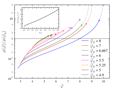
Figure 3: Shear modulus versus density for different glasses. Same styles as Fig. 1. In the inset we report $\mu(\widehat{\varphi}_{g})$ versus $\widehat{\varphi}_{g}$. Note that the dilatancy $R/\rho=(1/2)\widehat{\varphi}\partial\mu/\partial\widehat{\varphi}$ diverges both at jamming and at the low density spinodal point where the glass melts (see the Appendix).

For a glass selected at $\varphi_{g}$, when the density is higher than $\varphi_{G}$, the RS calculation we perform is incorrect. One should perform a full replica symmetry breaking (fRSB) computation Barrat et al. (1997); Zdeborová and Krzakala (2010); Charbonneau et al. (2014a). We leave this for future work, but we observe that for large enough $\varphi_{g}$ the Gardner transition happens at very high pressure and in that case the RS calculation should be a good approximation to the glass EOS at all pressures. For small $\varphi_{g}$ instead, the RS calculation gives a wrong prediction, namely the existence of an unphysical spinodal point at which the glass disappears. We expect, based on the analogy with the results of Zdeborová and Krzakala (2010), that a fRSB calculation will fix this problem.

A given glass prepared at $\varphi_{g}$ can be also followed in decompression, by decompressing at a relatively fast rate $\tau_{\rm dec}$ such that $\tau_{\rm vib}\ll\tau_{\rm dec}\ll\tau_{\rm exp}$. In this case we observe hysteresis (Fig. 1), consistently with experimental results Dyre (2006); Swallen et al. (2007); Singh et al. (2013). In fact, the glass pressure becomes lower than the liquid one, until upon decreasing density a spinodal point is reached, at which the glass becomes unstable and melts into the liquid Mariani et al. . Note that pressure “undershoots” (it has a local minimum, see Fig. 1) before the spinodal is reached Mariani et al. .

Results: shear –

We investigate now the response of glasses to a shear-strain perturbation. We consider a system compressed in equilibrium up to a density $\widehat{\varphi}_{g}$, where it remains stuck into a glass. Now, instead of compressing the system, we apply a shear-strain $\gamma$. In Fig. 2 we report the behavior of shear-stress $\sigma$ and pressure $p$ versus $\gamma$. At small $\gamma$ we observe a linear response elastic regime where $\sigma$ increases linearly with $\gamma$, $\sigma\sim\mu\gamma$ and pressure increases quadratically above the equilibrium liquid value, $p(\gamma)\sim p(\gamma=0)+(\beta R/\rho)\gamma^{2}$. Both the shear modulus $\mu$ and the dilatancy $R>0$ increase with $\widehat{\varphi}_{g}$, indicating that glasses prepared by slower annealing are more rigid.

Upon further increasing $\gamma$, glasses enter a non-linear regime, and undergo a Gardner transition at $\gamma_{G}(\varphi_{g})$ (Fig. 2). Like in compression, we find $\gamma_{G}(\varphi_{\rm d})=0$, and $\gamma_{G}$ increases rapidly with $\varphi_{g}$. For $\gamma>\gamma_{G}(\varphi_{\rm d})$, the glass breaks into subbasins and a fRSB calculation is needed. Note that the RS computation predicts a stress overshoot, followed by a spinodal point where the glass basin disappears. We expect that the fRSB computation gives similar results. The spinodal point corresponds to the point where the glass yields and starts to flow. The values of yield strain $\gamma_{\rm Y}$ and of yield stress $\sigma_{\rm Y}$ are also found to increase with $\varphi_{g}$. These results are qualitatively consistent with the experimental and numerical observations of Rodney et al. (2011); Koumakis et al. (2012).

Results: compression followed by shear –

One could also consider the case where (i) a liquid is slowly compressed up to $\varphi_{g}$ where it forms a glass, (ii) the glass is compressed up to a certain pressure $p$ (Fig. 1) and then (iii) a shear-strain $\gamma$ is applied. The response to shear-strain of these glasses compressed out of equilibrium is qualitatively similar to the one reported in Fig. 2, and we do not report the corresponding curves. Instead, we report in Fig. 3 the behavior of shear modulus $\mu$ as a function of density $\varphi$ for different glasses prepared at different $\varphi_{g}$. For each glass, we find that under compression $\mu$ increases with density, and diverges at the jamming point where $p\rightarrow\infty$. Note that, as discussed above and in Charbonneau et al. (2014a), describing the behavior around the jamming density requires a fRSB computation, that we did not perform here.

A useful thermodynamic identity gives the dilatancy $R/\rho=(1/2)\varphi\partial\mu/\partial\varphi$ Tighe (2014) (see the Appendix). This implies that the singular behavior of the shear modulus around jamming, which itself is well captured by a fRSB computation Yoshino and Zamponi (2014), should be directly reflected to the dilatancy, as pointed out in Tighe (2014). Further work is needed to understand experimental and numerical results Ren et al. (2013); Coulais et al. (2014); Otsuki and Hayakawa (2014).

Conclusions –

We have applied the state following procedure, developed in the context of spin glasses Franz and Parisi (1995); Barrat et al. (1997); Zdeborová and Krzakala (2010); Krzakala and Zdeborová (2013), to a microscopic model of glass former, namely hard spheres. We considered for simplicity the limit $d\rightarrow\infty$, where the method we used is exact, but the calculations can be generalized to obtain approximated quantitative predictions in finite $d$. According to Parisi and Zamponi (2010); Berthier et al. (2011), the simplest approximation is to use the results reported in this paper, replacing $\widehat{\varphi}=2^{d}\varphi/(d\,y^{\rm liq}_{\rm HS}(\varphi))$, $y^{\rm liq}_{\rm HS}(\varphi)$ being the contact value of the pair correlation function in the liquid phase, which can be obtained from a generalized Carnahan-Starling liquid EOS Charbonneau et al. (2011). This approximation is expected to be good at large $\varphi_{g}$, but gives poor results for $\varphi_{g}\sim\varphi_{\rm d}$. Systematic improvements over this approximation can be obtained following the ideas of Parisi and Zamponi (2010). It is clear, anyway, that the qualitative shape of the curves we obtained in $d\rightarrow\infty$ will not change in finite $d$, which is also supported by the numerical simulations of Charbonneau et al. (2011).

We did not attempt here a more precise quantitative comparison with experimental and numerical data, which we leave for future work, but we showed that the state following method is able to give predictions for many physical observables of experimental interest, and reproduces a quite large number of observations. These include: (i) the pressure as a function of density for different glasses (Fig. 1), which displays a jump in compressibility at $\varphi_{g}$ Parisi and Zamponi (2010); Charbonneau et al. (2011); (ii) the presence of hysteresis and of a spinodal point in decompression in the pressure-density curves (Fig. 1), where we show that more stable glasses (those with higher $\varphi_{g}$) display a larger hysteresis, consistently with the experimental observation of Dyre (2006); Swallen et al. (2007); Singh et al. (2013); the behavior of pressure and shear-stress under a shear-strain perturbation (Fig. 2), where we show that (iii) the shear modulus and the dilatancy increase for more stable glasses (higher $\varphi_{g}$), and (iv) that the shear-stress overshoots before a spinodal (yielding) point is reached where the glass yields and starts to flow (Fig. 2) Rodney et al. (2011); Koumakis et al. (2012). Note however that the spinodal (yield) point falls beyond the Gardner transition and therefore its estimate, reported in Fig. 2, is only approximate, a correct computation requires fRSB Charbonneau et al. (2014a). Furthermore, (v) we predict that glasses undergo a Gardner transition both in compression (Fig. 1) and in shear (Fig. 2), and we locate the Gardner transition point (see the Appendix). Finally, we (vi) compute the dilatancy and the shear modulus everywhere in the glass phase (Fig. 3 and the Appendix) and their behavior close to the jamming transition (see the Appendix).

This approach thus provides a coherent picture of the phase diagram of glasses in different regimes, under compression and under shear-strain, at moderate densities close to the dynamical glass transition and at high densities (pressures) close to jamming. Future work should be directed towards performing systematic comparisons between theory and experiment, and improving the theory, first by performing the fRSB computation, and second by improving the approximation in finite dimensions.

Acknowledgments –

We thank G. Biroli, P. Charbonneau, O. Dauchot, S. Franz, Y. Jin, F. Krzakala, J. Kurchan, M. Mariani, G. Parisi, F. Ricci-Tersenghi and L. Zdeborová, for many useful discussions. This work was supported by KAKENHI (No. 25103005 “Fluctuation & Structure” and No. 50335337) from MEXT, Japan, by JPS Core-to-Core Program “Non-equilibrium dynamics of soft matter and informations”, and by the European Research Council through ERC grant agreement No. 247328 and NPRGGLASS.

Contents

1. A The Franz-Parisi free energy
   1. A.1 Replicated entropy
   2. A.2 The entropic term
   3. A.3 The interaction term
      1. A.3.1 General expression of the replicated Mayer function
      2. A.3.2 Computation of the interaction term for a RS displacement matrix
   4. A.4 Final result for the internal entropy of the planted state
   5. A.5 Derivation from the Gaussian replica method
   6. A.6 Stability of the RS solution
      1. A.6.1 The structure of the unstable mode
      2. A.6.2 Entropic term part of the stability matrix
      3. A.6.3 The interaction part term of the stability matrix
      4. A.6.4 The stability matrix in presence of the shear
      5. A.6.5 The replicon eigenvalue
2. B Computation of physical observables
   1. B.1 Maximization of the entropy
   2. B.2 Pressure and shear stress
   3. B.3 Response to an infinitesimal strain
3. C Special limits and approximations
   1. C.1 Constrained replicas in equilibrium
   2. C.2 Perturbative solution for small $\eta$ and $\gamma$
   3. C.3 The jamming limit
   4. C.4 Following states under compression: approximation $\Delta^{f}=0$
      1. C.4.1 Pressure and thermodynamic relations
      2. C.4.2 The jamming limit
4. D Results
   1. D.1 Compression
   2. D.2 Shear
   3. D.3 Quality of the approximation $\Delta^{f}=0$
5. E Comparison with previous work

Appendix A The Franz-Parisi free energy

The Franz-Parisi potential allows one to compute the properties of an individual glassy state. We consider a set of $m$ coupled “reference” replicas $R^{1},\cdots,R^{m}$, where $R=\{r_{i}\}$ is a configuration of the system. These $m$ replicas interact with a potential energy $V(R)=\sum_{i<j}v(r_{i}-r_{j})$, at temperature $T_{g}$ (with $k_{B}=1$), and are used to select a glassy state, following Monasson (1995). At equilibrium we shall consider $m=1$, while out of equilibrium states can be selected using $m\neq 1$. In this paper we write the formulae for general $m$, but we will only report results for $m=1$. Furthermore, we consider an additional “constrained” replica $X=\{x_{i}\}$, which is coupled to one of the $m$ replicas and is used to probe the glassy state selected by the reference replicas. This constrained replica has potential energy $V_{\gamma}(X)=\sum_{i<j}v_{\gamma}(x_{i}-x_{j})$, where the suffix $\gamma$ is there to indicate the possible presence of perturbations (e.g. a shear strain), and temperature $T$. We define the mean square displacement as

$$\Delta(X,R)=\frac{d}{N}\sum_{i=1}^{N}(x_{i}-r_{i})^{2}\ .$$ (1)

The factor of $d$ is added to ensure that $\Delta(X,R)$ has a finite limit for $d\rightarrow\infty$ Parisi and Zamponi (2010); Kurchan et al. (2012, 2013); Charbonneau et al. (2014b).

In the following we restrict the discussion to a mean-field setting in which metastable states have infinite life-time and phase coexistence is absent (see Mézard and Parisi (2000) for a discussion of phase coexistence in this context). This is exactly realized in the limit $d\rightarrow\infty$ Parisi and Zamponi (2010); Kurchan et al. (2012, 2013); Charbonneau et al. (2014b) and can be taken as an approximation for finite $d$. We want to compute the free energy of the constrained replica, and average over the reference replicas:

$$\begin{split}Z_{g}[R,\Delta^{r}]&=\int dXe^{-\beta V_{\gamma}(X)}\delta(\Delta^{r}-\Delta(X,R))\ ,\\ F_{g}[T,\gamma;R,\Delta^{r}]&=-T\log\int dXe^{-\beta V_{\gamma}(X)}\delta(\Delta^{r}-\Delta(X,R))\equiv-T\log Z_{g}\ ,\\ Z_{m}&=\int dR^{1}\cdots dR^{m}\,e^{-\beta_{g}\sum_{a=1}^{m}V(R^{a})}\ ,\\ F_{g}[T,\gamma;\Delta^{r}]&=\overline{F_{g}[T,\gamma;R,\Delta^{r}]}\equiv\frac{1}{Z_{m}}\int dR^{1}\cdots dR^{m}\,e^{-\beta_{g}\sum_{a=1}^{m}V(R^{a})}F_{g}[T,\gamma;R^{1},\Delta^{r}]\ .\end{split}$$ (2)

Note that the above definition of $F_{g}[T,\gamma;R,\Delta^{r}]$ is slightly different from the one we have given in the main text, because we replaced the Heaviside step function with a Dirac delta function. With this choice, $F_{g}[T,\gamma;\Delta^{r}]$ is the averaged (over glassy states) large deviation function of the mean square displacement $\Delta^{r}$: it gives the thermodynamic weight of all the configurations of $X$ that are at distance $\Delta^{r}$ from $R$. Above the dynamical packing fraction $\varphi_{\rm d}$ where the first glassy states appear, the free energy $F_{g}[T,\gamma;\Delta^{r}]$ develops a minimum at a finite value of $\Delta^{r}$, signaling the presence of metastable states. The intuitive reason for the presence of a secondary minimum in the glass phase is the following. At very small $\Delta^{r}$, there are few configurations, so the weight is small and $F_{g}[T,\gamma;\Delta^{r}]$. Upon increasing $\Delta^{r}$, the weight increases as one explores larger portions of the glass basin around $R$, and $F_{g}[T,\gamma;\Delta^{r}]$ decreases. However, if $\Delta^{r}$ is increased beyond the size of the glass basins, then the configurations at distance $\Delta^{r}$ are on the barriers that surround the glassy state, therefore the weight is small and $F_{g}[T,\gamma;\Delta^{r}]$ increases again. Only at much larger $\Delta^{r}$, when all the configurations corresponding to other glass basins are included, the entropic contribution of all the glass basins makes $F_{g}[T,\gamma;\Delta^{r}]$ smaller. See Franz and Parisi (1995); Barrat et al. (1997) for a more detailed discussion, and Mézard and Parisi (2000) for a detailed discussion of how to construct $F_{g}[T,\gamma;\Delta^{r}]$ by adding a coupling to the system, and for a generalization to this discussion to finite $d$ by taking into account phase coexistence.

Minimizing the constrained free energy $F_{g}[T,\gamma;\Delta^{r}]$ with respect to $\Delta^{r}$ is thus the way to obtain the properties of the typical metastable states selected by the reference configuration $R$ once followed under an external perturbation Franz and Parisi (1995); Barrat et al. (1997); Mézard and Parisi (1999, 2000). At the minimum, the value of $\Delta^{r}$ corresponds to the configurations that have larger Boltzmann weight in the glass basin, and $F_{g}[T,\gamma;\Delta^{r}]$ gives the corresponding weight. The weight of configurations corresponding to smaller $\Delta^{r}$ is exponentially suppressed when $d\rightarrow\infty$. Therefore in the following we assume that $\Delta^{r}$ is determined by the minimization of the free energy. Note that if we define the constrained free energy with a “soft” constraint (a Heaviside $\theta$ function, as in the main text) instead of a “hard” constraint (a Dirac $\delta$ function), we will get the same value for the saddle point solution for the mean square displacement and the same properties for the metastable states because the configurations that we are adding by considering a soft constraint have an exponentially suppressed weight. This is why we have chosen to use the $\theta$ function in the main text, because it is better for illustrative purposes.

We can use the replica trick to compute the logarithm. If we define

$$\begin{split}-\beta NF_{\rm FP}&=\log\int dR^{1}\cdots dR^{m}dX^{1}\cdots dX^{s}e^{-\beta_{g}\sum_{a=1}^{m}V(R^{a})-\beta\sum_{b=1}^{s}V_{\gamma}(X^{b})}\\ &=\log\int dX^{1}\cdots dX^{m}e^{-\beta_{g}\sum_{a=1}^{m}V(X^{a})}(Z_{g})^{s}=\log[Z_{m}\overline{(Z_{g})^{s}}]\ ,\end{split}$$ (3)

then we have, at leading order for small $s$

$$\begin{split}-\beta NF_{\rm FP}&=\log\left[Z_{m}\overline{(Z_{g})^{s}}\right]\sim\log\left[Z_{m}(1+s\overline{\log(Z_{g})}+O(s^{2}))\right]=\log Z_{m}+s\,\overline{\log Z_{g}}+O(s^{2})\\ &=-\beta F_{m}-s\beta F_{g}[T,\gamma]+O(s^{2})\ .\end{split}$$ (4)

Therefore we have to compute the free energy of $m+s$ replicas; $m$ “reference” ones and $s$ “constrained” ones, that are at different temperature or density. Then we have to send $s\rightarrow 0$; the leading order gives the Monasson replicated free energy $F_{m}$ Monasson (1995), while the linear order in $s$ gives the Franz-Parisi free energy $F_{g}[T,\gamma]$ Franz and Parisi (1995). In this paper we will only consider the case $m\rightarrow 1$, in which $F_{m}$ coincides with the liquid free energy.

In the following we consider a system of hard spheres in $d\rightarrow\infty$, hence temperature plays no role and density (or packing fraction) is the only relevant control parameter. Furthermore, the energy is zero, therefore the free energy contains only the entropic term $-\beta F=s$. For technical reasons, it is convenient to fix the packing fraction through the sphere diameters, while assuming that the number density is constant, as in the Lubachevsky-Stillinger algorithm Lubachevsky and Stillinger (1990). We consider that the $m$ reference replicas have diameter $D_{g}$ and packing fraction $\varphi_{g}$, while the $s$ constrained replicas have the same number density but $D=D_{g}(1+\eta/d)$. Following Parisi and Zamponi (2010); Kurchan et al. (2012) we also define a rescaled packing fraction $\widehat{\varphi}=2^{d}\varphi/d$ that has a finite limit when $d\rightarrow\infty$. Note that the packing fraction of the constrained replicas is therefore $\varphi=\varphi_{g}(D/D_{g})^{d}\sim\varphi_{g}e^{\eta}$ and similarly $\widehat{\varphi}=\widehat{\varphi}_{g}e^{\eta}$.

Following Yoshino and Mézard (2010); Yoshino (2012); Yoshino and Zamponi (2014), we also apply a shear strain $\gamma$ to the constrained replicas, which is obtained by deforming linearly the volume in which the system is contained. We call $x^{\prime}_{\mu}$, with $\mu=1,\cdots,d$, the coordinates in the original reference frame, in which the shear strain is applied. In this frame, the cubic volume is deformed because of shear strain. To remove this undesirable feature, we introduce new coordinates $x_{\mu}$ of a “strained” frame in which the volume is brought back to a cubic shape. If the strain is applied along direction $\mu=2$, then all the coordinates are unchanged, $x_{\mu}=x_{\mu}^{\prime}$, except the first one which is changed according to

$$x_{1}^{\prime}=x_{1}+\gamma x_{2}\ ,\hskip 30.0ptx_{1}=x_{1}^{\prime}-\gamma x_{2}^{\prime}\ .$$ (5)

Let us call $S(\gamma)$ the matrix such that $x^{\prime}=S(\gamma)x$. In the original frame (where the volume is deformed by strain), two particles of the slave replica interact with the potential $v(|x^{\prime}-y^{\prime}|)$. If we change variable to the strained frame (where the volume is not deformed), the interaction is

$$v_{\gamma}(x-y)=v(|S(\gamma)(x-y)|)\ .$$ (6)

An important remark is that $\det S(\gamma)=1$ meaning that the simple strain defined above does not change the volume and thus the average density $\rho=N/V$ of the system.

In summary, if we consider following a glass state under a compression and a strain, we have to compute the Franz-Parisi potential where the constrained replicas have a diameter $D=D_{g}(1+\eta/d)$ and interact with a potential $V_{\gamma}(X)=\sum_{i<j}v_{\gamma}(x_{i}-x_{j})$. The control parameter of the reference replica is their density $\varphi_{g}$, while the control parameters of the constrained replicas are compression rate $\eta=\log(\varphi/\varphi_{g})$ and shear strain $\gamma$. The replicated entropy of this system can be computed through a generalization of the methods of Refs. Kurchan et al. (2012, 2013), which we present below.

A.1 Replicated entropy

The replicated entropy of the system for a generic replica structure has been derived in Kurchan et al. (2013):

$$s[\hat{\alpha}]=1-\log\rho+d\log(m+s)+\frac{(m+s-1)d}{2}\log(2\pi eD_{g}^{2}/d^{2})+\frac{d}{2}\log\det(\hat{\alpha}^{m+s,m+s})-\frac{d}{2}\widehat{\varphi}_{g}\,{\cal F}\left(2\hat{\alpha}\right)\ ,$$ (7)

where $\hat{\alpha}=d\left\langle u_{a}\cdot u_{b}\right\rangle/D_{g}^{2}$ is a $(m+s)\times(m+s)$ symmetric matrix and $\hat{\alpha}^{a,a}$ is the matrix obtained from $\hat{\alpha}$ by deleting the $a$-th row and column. The matrix $\hat{\alpha}$ encodes the fluctuations of the replica displacements $u_{a}$ around the center of mass of all replicas. Because $\sum_{a}u_{a}=0$, the sum of each row and column of $\hat{\alpha}$ is equal to zero, i.e. $\hat{\alpha}$ is a Laplacian matrix. Here we used $D_{g}$ as the unit of length and for this reason $D_{g}$ and $\widehat{\varphi}_{g}$ appear in Eq. (7). We call the last term in Eq. (7) the “interaction term”, while all the rest will be called the “entropic term”.

Given the replica structure of the problem, the simplest replica symmetric (RS) ansatz for the matrix $\hat{\alpha}$ is

$$\begin{split}\hat{\alpha}=&\begin{bmatrix}\delta^{g}&-\alpha^{g}&\cdots&-\alpha^{g}&-\chi&\lx@intercol\hfil\cdots\hfil\lx@intercol&-\chi\\ -\alpha^{g}&\delta^{g}&\cdots&-\alpha^{g}&&\lx@intercol\hfil\hfil\lx@intercol&\\ \vdots&\ddots&\ddots&\vdots&\vdots&\lx@intercol\hfil\hfil\lx@intercol&\vdots\\ -\alpha^{g}&\cdots&-\alpha^{g}&\delta^{g}&-\chi&\lx@intercol\hfil\cdots\hfil\lx@intercol&-\chi\\ -\chi&\lx@intercol\hfil\cdots\hfil\lx@intercol&-\chi&\delta&-\alpha&\lx@intercol\hfil\cdots\hfil\lx@intercol&-\alpha\\ &&&&-\alpha&\delta&\lx@intercol\hfil\cdots\hfil\lx@intercol&-\alpha\\ \vdots&&&\vdots&\vdots&\vdots&&\ddots&&\vdots\\ &&&&-\alpha&\lx@intercol\hfil\cdots\hfil\lx@intercol&\delta&-\alpha\\ -\chi&\lx@intercol\hfil\cdots\hfil\lx@intercol&-\chi&-\alpha&\lx@intercol\hfil\cdots\hfil\lx@intercol&-\alpha&\delta\\ \end{bmatrix}\\ \\ &\delta^{g}=(m-1)\alpha^{g}+s\chi\\ &\delta=(s-1)\alpha+m\chi\\ \end{split}$$ (8)

Note that the mean square displacements between the replicas are $\Delta_{ab}=d\left\langle(u_{a}-u_{b})^{2}\right\rangle/D_{g}^{2}=\alpha_{aa}+\alpha_{bb}-2\alpha_{ab}$ (we scaled $\hat{\Delta}$ by $D_{g}$ because we use $\Delta_{g}$ as the unit of length) and therefore the matrix $\hat{\Delta}$ has the form

$$\hat{\Delta}=\begin{bmatrix}0&\Delta^{g}&\cdots&\Delta^{g}&\Delta^{r}&\lx@intercol\hfil\cdots\hfil\lx@intercol&\Delta^{r}\\ \Delta^{g}&0&\cdots&\Delta^{g}&&\lx@intercol\hfil\hfil\lx@intercol&\\ \vdots&\ddots&\ddots&\vdots&\vdots&\lx@intercol\hfil\hfil\lx@intercol&\vdots\\ \Delta^{g}&\cdots&\Delta^{g}&0&\Delta^{r}&\lx@intercol\hfil\cdots\hfil\lx@intercol&\Delta^{r}\\ \Delta^{r}&\lx@intercol\hfil\cdots\hfil\lx@intercol&\Delta^{r}&0&\Delta&\lx@intercol\hfil\cdots\hfil\lx@intercol&\Delta\\ &&&&\Delta&0&\lx@intercol\hfil\cdots\hfil\lx@intercol&\Delta\\ \vdots&&&\vdots&\vdots&\vdots&&\ddots&&\vdots\\ &&&&\Delta&\lx@intercol\hfil\cdots\hfil\lx@intercol&0&\Delta\\ \Delta^{r}&\lx@intercol\hfil\cdots\hfil\lx@intercol&\Delta^{r}&\Delta&\lx@intercol\hfil\cdots\hfil\lx@intercol&\Delta&0\\ \end{bmatrix}$$ (9)

with

$$\begin{split}&\Delta^{g}=2(\delta^{g}+\alpha^{g})=2(m\alpha^{g}+s\chi)\ ,\\ &\Delta=2(\delta+\alpha)=2(s\alpha+m\chi)\,\\ &\Delta^{r}=\delta^{g}+\delta+2\chi=(m-1)\alpha^{g}+(s-1)\alpha+(m+s+2)\chi\ ,\\ &\Delta^{f}=2\Delta^{r}-\Delta^{g}-\Delta=2(2\chi-\alpha^{g}-\alpha)\ ,\end{split}$$ (10)

where $\Delta^{g}$ is internal to the block of $m$ replicas, $\Delta$ to the $s$ replicas, and $\Delta^{r}$ is the relative displacement between the $m$-type and $s$-type replicas. Finally, we introduced $\Delta^{f}$ which measures the additional fluctuations between the $m$ and $s$-type replicas. The entropy (7) must be maximized with respect to $\Delta^{g},\Delta,\Delta^{r}$.

A.2 The entropic term

We want to compute $\det\hat{\alpha}^{m+s,m+s}$, where we recall that $\hat{\alpha}^{a,a}$ is the matrix obtained from $\hat{\alpha}$ by deleting the $a$-th row and column, i.e. it is the $(a,a)$-cofactor of $\hat{\alpha}$. Begin Laplacian, $\hat{\alpha}$ has a vanishing determinant. Also, the “Kirchhoff’s matrix tree theorem” states that for Laplacian matrices, all the cofactors are equal, hence $\det\hat{\alpha}^{a,a}$ is independent of $a$. Therefore, if $\mathbf{1}$ is the identity in $m+s$ dimensions, we have

$$\det(\hat{\alpha}+\varepsilon\mathbf{1})=\det\hat{\alpha}+\varepsilon\sum_{a=1}^{m+s}\det\hat{\alpha}^{a,a}+O(\varepsilon^{2})\ \ \ \Rightarrow\ \ \ \det\hat{\alpha}^{a,a}=\lim_{\varepsilon\rightarrow 0}\frac{1}{\varepsilon(m+s)}\det(\hat{\alpha}+\varepsilon\mathbf{1})\ .$$ (11)

We then define $\hat{\beta}(\varepsilon)=\hat{\alpha}+\varepsilon\mathbf{1}$ and we note that

$$\hat{\beta}(\varepsilon)=\begin{pmatrix}A&B\\ B^{T}&D\end{pmatrix}$$ (12)

where $A$ is a $m\times m$ matrix with components $A_{ab}=(\delta^{g}+\alpha^{g}+\varepsilon)\delta_{ab}-\alpha^{g}$, $D$ is a $s\times s$ matrix with $D_{ab}=(\delta+\alpha+\varepsilon)\delta_{ab}-\alpha$, and $B$ is a $m\times s$ matrix with $B_{ab}=\chi$.

We can use the following general formula

$$\det\hat{\beta}(\varepsilon)=(\det A)\det(D-B^{T}A^{-1}B)\ ,$$ (13)

recalling that a $m\times m$ matrix $M_{ab}=M_{1}\delta_{ab}+M_{2}$ has determinant $\det M=M_{1}^{m-1}(M_{1}+mM_{2})$ and its inverse is $M^{-1}_{ab}=(M^{-1})_{1}\delta_{ab}+(M^{-1})_{2}$ with

$$\begin{split}(M^{-1})_{1}&=\frac{1}{M_{1}}\ ,\\ (M^{-1})_{2}&=-\frac{M_{2}}{M_{1}(M_{1}+mM_{2})}\ .\end{split}$$ (14)

The matrix $A^{-1}$ has this form, with

$$\begin{split}(A^{-1})_{1}&=\frac{1}{\alpha^{g}+\delta^{g}+\varepsilon}\ ,\\ (A^{-1})_{2}&=\frac{\alpha^{g}}{(\alpha^{g}(1-m)+\delta^{g}+\varepsilon)(\alpha^{g}+\delta^{g}+\varepsilon)}\ ,\\ \det A&=\left(\delta^{g}+\alpha^{g}+\varepsilon\right)^{m-1}\left(\delta^{g}+(1-m)\alpha^{g}+\varepsilon\right)\ .\end{split}$$ (15)

The matrix $\Omega=D-B^{T}A^{-1}B$ has the same form with

$$\begin{split}\Omega_{1}&=\delta+\varepsilon+\alpha\ ,\\ \Omega_{2}&=-\alpha-\chi^{2}[m(A^{-1})_{1}+m^{2}(A^{-1}_{2})]\ ,\\ \det\Omega&=(\delta+\alpha+\varepsilon)^{s-1}\{\delta+\alpha(1-s)+\epsilon-s\chi^{2}[m(A^{-1})_{1}+m^{2}(A^{-1}_{2})]\}\ .\end{split}$$ (16)

Using Eqs. (15), (16), (13) and (11), we obtain the final result

$$\begin{split}\det\hat{\alpha}^{(m+s,m+s)}&=\chi(m\alpha^{g}+s\chi)^{m-1}(s\alpha+m\chi)^{s-1}\ .\end{split}$$ (17)

A.3 The interaction term

Here we compute the interaction function ${\cal F}(2\hat{\alpha})$. This function has been computed in Kurchan et al. (2012), but only for $\eta=0$ and $\gamma=0$. Here we need to generalize the calculation to non-zero perturbations.

A.3.1 General expression of the replicated Mayer function

We follow closely the derivation of Kurchan et al. (2012) which has been generalized in Yoshino and Zamponi (2014) to the presence of a strain. The replicated Mayer function is

$$\begin{split}\overline{f}(\bar{u})&=\int dX\left\{-1+\prod_{a=1}^{m}\theta(|X+u_{a}|-D_{g})\prod_{b=m+1}^{m+s}\theta(|S(\gamma)(X+u_{b})|-D)\right\}\\ &=-\int dX\,\theta\left(\max_{a=1,m+s}\{D_{a}-|S(\gamma_{a})(X+u_{a})|\}\right)\ ,\end{split}$$ (18)

where we introduced $D_{a}=D_{g}(1+\eta_{a}/d)$ with $\eta_{a}=\gamma_{a}=0$ for $1\leq a\leq m$, and $\eta_{a}=\eta$ and $\gamma_{a}=\gamma$ for $m+1\leq a\leq m+s$.

The $u_{a}$ are $m+s$ vectors in $d$ dimensions and define a hyperplane in the $d$-dimensional space. It is then reasonable to assume that this $(m+s)$-dimensional plane is orthogonal to the strain directions $\mu=1,2$ with probability going to 1 for $d\rightarrow\infty\gg m+s$. Hence, the vector $X$ can be decomposed in a two dimensional vector $\{X_{1},X_{2}\}$ parallel to the strain plane, a $(d-m-s-2)$-component vector $X_{\perp}$, orthogonal to the plane $\mu=1,2$ and to the plane defined by $u_{a}$, and a $m+s$-component vector $X_{\parallel}$ parallel to that plane. Defining $\Omega_{d}$ as the $d$-dimensional solid angle and recalling that $V_{d}=\Omega_{d}/d$, and following the same steps as in (Kurchan et al., 2012, Sec. 5), we have, calling $k=m+s$

$$\begin{split}\overline{f}(\bar{u})&=-\int dX_{1}dX_{2}\ d^{k}X_{\parallel}\ d^{d-k-2}X_{\perp}\ \theta\left(\max_{a}\{D_{a}^{2}-(X_{1}+\gamma_{a}X_{2})^{2}-X_{2}^{2}-|X_{\parallel}+u_{a}|^{2}-|X_{\perp}|^{2}\}\right)\\ &=-\Omega_{d-k-2}\int dX_{1}dX_{2}\ d^{k}X_{\parallel}\int_{0}^{\infty}dx\,x^{d-k-3}\,\theta\left(\max_{a}\{D_{a}^{2}-x^{2}-(X_{1}+\gamma_{a}X_{2})^{2}-X_{2}^{2}-|X_{\parallel}+u_{a}|^{2}\}\right)\\ &=-\Omega_{d-k-2}\int dX_{1}dX_{2}\ d^{k}X_{\parallel}\int_{0}^{\sqrt{\max_{a}\{D_{a}^{2}-(X_{1}+\gamma_{a}X_{2})^{2}-X_{2}^{2}-|X_{\parallel}+u_{a}|^{2}\}}}dx\,x^{d-k-3}\\ &=-V_{d-k-2}\int dX_{1}dX_{2}\ d^{k}X_{\parallel}\,\Theta_{d-k-2}\left(\max_{a}\{D_{a}^{2}-(X_{1}+\gamma_{a}X_{2})^{2}-X_{2}^{2}-|X_{\parallel}+u_{a}|^{2}\}\right)\end{split}$$ (19)

where we defined the function $\Theta_{p}(x)=x^{p/2}\theta(x)$.

It has been shown in Kurchan et al. (2012) that the region where $\overline{f}(\bar{u})$ has a non-trivial dependence on the $u_{a}$ is where $u_{a}\sim 1/\sqrt{d}$. Here we use $D_{g}$ as the unit of length, hence we define $u_{a}=x_{a}D_{g}/\sqrt{d}$, $X_{1,2}=\zeta_{1,2}D_{g}/\sqrt{d}$ and $X_{\parallel}=\epsilon D_{g}/\sqrt{d}$. Using that $\lim_{n\rightarrow\infty}\Theta_{n}(1+y/n)=e^{y/2}$, and that for large $d$ and finite $k$ we have $V_{d-k}/V_{d}\sim d^{k/2}/(2\pi)^{k/2}$, we have

$$\begin{split}\overline{f}(\bar{u})&=-\frac{V_{d-k-2}}{V_{d}}\frac{V_{d}D_{g}^{d}}{d^{(k+2)/2}}\int d\zeta_{1}d\zeta_{2}d^{k}\epsilon\,\Theta_{d-k-2}\left(1-\frac{1}{d}\min_{a}\{-2\eta_{a}+(\zeta_{1}+\gamma_{a}\zeta_{2})^{2}+\zeta_{2}^{2}+|\epsilon+x_{a}|^{2}\}\right)\\ &\sim-V_{d}D_{g}^{d}\int\frac{d\zeta_{1}d\zeta_{2}d^{k}\epsilon}{(2\pi)^{(k+2)/2}}\,e^{-\frac{1}{2}\min_{a}\{-2\eta_{a}+(\zeta_{1}+\gamma_{a}\zeta_{2})^{2}+\zeta_{2}^{2}+|\epsilon+x_{a}|^{2}\}}\equiv-V_{d}D_{g}^{d}{\cal F}(\bar{x})\ ,\end{split}$$ (20)

where the function ${\cal F}$ has been introduced following Kurchan et al. (2012, 2013).

We can then follow the same steps as in (Kurchan et al., 2013, Sec.V C) and in Yoshino and Zamponi (2014) to obtain

$$\begin{split}\mathcal{F}(\bar{x})&=\int\frac{d\zeta_{1}d\zeta_{2}d^{k}\epsilon}{(2\pi)^{(k+2)/2}}\,e^{-\frac{1}{2}\min_{a}\{-2\eta_{a}+(\zeta_{1}+\gamma_{a}\zeta_{2})^{2}+\zeta_{2}^{2}+|\epsilon+x_{a}|^{2}\}}\\ &=\int\frac{d\zeta_{1}d\zeta_{2}d^{k}\epsilon}{(2\pi)^{(k+2)/2}}\lim_{n\rightarrow 0}\left(\sum_{a=1}^{k}e^{-\frac{1}{2n}[-2\eta_{a}+(\zeta_{1}+\gamma_{a}\zeta_{2})^{2}+\zeta_{2}^{2}+|\epsilon+x_{a}|^{2}]}\right)^{n}\\ &=\lim_{n\rightarrow 0}\sum_{n_{1},\ldots,n_{k};\sum_{a=1}^{k}n_{a}=n}\frac{n!}{n_{1}!\ldots n_{k}!}\int\frac{d\zeta_{1}d\zeta_{2}d^{k}\epsilon}{(2\pi)^{(k+2)/2}}e^{-\sum_{a}\frac{n_{a}}{2n}[-2\eta_{a}+(\zeta_{1}+\gamma_{a}\zeta_{2})^{2}+\zeta_{2}^{2}+|\epsilon+x_{a}|^{2}]}\\ \\ &=\lim_{n\rightarrow 0}\sum_{n_{1},\ldots,n_{k};\sum_{a=1}^{k}n_{a}=n}\frac{n!}{n_{1}!\ldots n_{k}!}e^{\sum_{a=1}^{k}\frac{n_{a}}{n}\eta_{a}-\frac{1}{2}\sum_{a=1}^{k}\frac{n_{a}}{n}|x_{a}|^{2}+\frac{1}{2}\sum_{a,b}^{1,k}\frac{n_{a}n_{b}}{n^{2}}x_{a}\cdot x_{b}}\int\frac{d\zeta_{1}d\zeta_{2}}{2\pi}e^{-\sum_{a}\frac{n_{a}}{2n}[(\zeta_{1}+\gamma_{a}\zeta_{2})^{2}+\zeta_{2}^{2}]}\\ &=\lim_{n\rightarrow 0}\sum_{n_{1},\ldots,n_{k};\sum_{a=1}^{k}n_{a}=n}\frac{n!}{n_{1}!\ldots n_{k}!}e^{\sum_{a=1}^{k}\frac{n_{a}}{n}\eta_{a}-\frac{1}{4}\sum_{a,b}^{1,k}\frac{n_{a}n_{b}}{n^{2}}(x_{a}-x_{b})^{2}}\int\frac{d\zeta}{\sqrt{2\pi}}e^{-\frac{\zeta^{2}}{2}\left[1+\frac{1}{2}\sum_{ab}\frac{n_{a}n_{b}}{n^{2}}(\gamma_{a}-\gamma_{b})^{2}\right]}\ .\end{split}$$ (21)

We now introduce the matrix $\hat{\Delta}$ of mean square displacements between replicas

$$\Delta_{ab}=(x_{a}-x_{b})^{2}=\frac{d}{D_{g}^{2}}(u_{a}-u_{b})^{2}\ .$$ (22)

We should now recall that the Mayer function is evaluated in $\bar{u}-\bar{v}$, hence after rescaling the function ${\cal F}$ is evaluated in $\bar{x}-\bar{y}$. For $d\rightarrow\infty$, the interaction term is dominated by a saddle point on $\bar{u}$ and $\bar{v}$, such that $(x_{a}-x_{b})^{2}=(y_{a}-y_{b})^{2}=\Delta_{ab}$ and $x_{a}\cdot y_{b}=0$ Kurchan et al. (2012, 2013); Charbonneau et al. (2014b), hence $(x_{a}-y_{a}-x_{b}+y_{b})^{2}=(x_{a}-x_{b})^{2}+(y_{a}-y_{b})^{2}=2\Delta_{ab}$. This is also why the function ${\cal F}$ is evaluated in $2\hat{\alpha}$ in Eq. (7). The contribution of the interaction term to the free energy (7) is Kurchan et al. (2012)

$$\frac{1}{2}\frac{N}{V}\overline{f}(\bar{u}-\bar{v})=-\frac{NV_{d}D_{g}^{d}}{2V}{\cal F}(\bar{x}-\bar{y})=-2^{d-1}\varphi_{g}{\cal F}(2\hat{\alpha})=-\frac{d\widehat{\varphi}_{g}}{2}{\cal F}(2\hat{\alpha})\ .$$ (23)

With an abuse of notation, we now call ${\cal F}(\hat{\Delta})={\cal F}(2\hat{\alpha})$.

We therefore obtain at the saddle point

$$\begin{split}\mathcal{F}(\hat{\Delta})&=\lim_{n\rightarrow 0}\sum_{n_{1},\ldots,n_{k};\sum_{a=1}^{k}n_{a}=n}\frac{n!}{n_{1}!\ldots n_{k}!}e^{\sum_{a=1}^{k}\frac{n_{a}}{n}\eta_{a}-\frac{1}{2}\sum_{a,b}^{1,k}\frac{n_{a}n_{b}}{n^{2}}\Delta_{ab}}\int\frac{d\zeta}{\sqrt{2\pi}}e^{-\frac{\zeta^{2}}{2}\left[1+\frac{1}{2}\sum_{ab}\frac{n_{a}n_{b}}{n^{2}}(\gamma_{a}-\gamma_{b})^{2}\right]}\\ &=\int\frac{d\zeta}{\sqrt{2\pi}}e^{-\frac{\zeta^{2}}{2}}\lim_{n\rightarrow 0}\sum_{n_{1},\ldots,n_{k};\sum_{a=1}^{k}n_{a}=n}\frac{n!}{n_{1}!\ldots n_{k}!}e^{\sum_{a=1}^{k}\frac{n_{a}}{n}\eta_{a}-\frac{1}{2}\sum_{a,b}^{1,k}\frac{n_{a}n_{b}}{n^{2}}\left(\Delta_{ab}+\frac{\zeta^{2}}{2}(\gamma_{a}-\gamma_{b})^{2}\right)}\\ &=\int\frac{d\zeta}{\sqrt{2\pi}}e^{-\frac{\zeta^{2}}{2}}{\cal F}_{0}\left(\Delta_{ab}+\frac{\zeta^{2}}{2}(\gamma_{a}-\gamma_{b})^{2}\right)\ ,\end{split}$$ (24)

where ${\cal F}_{0}(\hat{\Delta})$ is the interaction function in absence of strain and is given by

$${\cal F}_{0}(\hat{\Delta})=\lim_{n\rightarrow 0}\sum_{n_{1},\ldots,n_{k};\sum_{a=1}^{k}n_{a}=n}\frac{n!}{n_{1}!\ldots n_{k}!}e^{\sum_{a=1}^{k}\frac{n_{a}}{n}\eta_{a}-\frac{1}{2}\sum_{a,b}^{1,k}\frac{n_{a}n_{b}}{n^{2}}\Delta_{ab}}\ .$$ (25)

A.3.2 Computation of the interaction term for a RS displacement matrix

We now compute the function ${\cal F}_{0}(\hat{\Delta})$. for the replica structure encoded by the matrix (8). Defining $\Sigma_{m}=\sum_{a=1}^{m}\frac{n_{a}}{n}$ and $\Sigma_{s}=\sum_{a=m+1}^{m+s}\frac{n_{a}}{n}$, keeping in mind that $\Sigma_{m}+\Sigma_{s}=1$, and recalling that $\eta_{a}=\eta$ for $m+1\leq a\leq m+s$ and $\eta_{a}=0$ otherwise, we can then write with some manipulations

$$\begin{split}{\cal F}_{0}(\hat{\Delta})&=\lim_{n\rightarrow 0}\sum_{n_{1},\ldots,n_{m+s};\sum_{a=1}^{m+s}n_{a}=n}\frac{n!}{n_{1}!\ldots n_{m+s}!}e^{-\left(\frac{\Delta^{g}}{2}+\frac{\Delta^{f}}{2}\right)\Sigma_{m}-\left(\frac{\Delta}{2}-\eta\right)\Sigma_{s}+\frac{\Delta^{f}}{2}\Sigma_{m}^{2}+\frac{\Delta^{g}}{2}\sum_{a=1}^{m}\frac{n_{a}^{2}}{n^{2}}+\frac{\Delta}{2}\sum_{a=m+1}^{m+s}\frac{n_{a}^{2}}{n^{2}}}\ .\end{split}$$ (26)

We now introduce Gaussian multipliers to decouple the quadratic terms and introduce the notation ${\cal D}\lambda=\frac{d\lambda}{\sqrt{2\pi}}e^{-\lambda^{2}/2}$. Note that $\Delta^{g}\geq 0$ and $\Delta\geq 0$. Under the assumption that $2\Delta^{f}\geq 0$ (to be discussed later on), we get

$$\begin{split}{\cal F}_{0}(\hat{\Delta})&=\int{\cal D}\lambda_{a}{\cal D}\mu\lim_{n\rightarrow 0}\left[\sum_{a=1}^{m}e^{-\frac{1}{n}\left(\frac{\Delta^{g}}{2}+\frac{\Delta^{f}}{2}+\lambda_{a}\sqrt{\Delta^{g}}+\mu\sqrt{\Delta^{f}}\right)}+\sum_{a=m+1}^{m+s}e^{-\frac{1}{n}\left(\frac{\Delta}{2}-\eta+\lambda_{a}\sqrt{\Delta}\right)}\right]^{n}\\ &=\int{\cal D}\lambda_{a}{\cal D}\mu\,e^{-\min\left\{\frac{\Delta^{g}}{2}+\frac{\Delta^{f}}{2}+(\min_{a\leq m}\lambda_{a})\sqrt{\Delta^{g}}+\mu\sqrt{\Delta^{f}},\,\frac{\Delta}{2}-\eta+(\min_{a>m}\lambda_{a})\sqrt{\Delta}\right\}}\end{split}$$ (27)

Now we use that for any function $f(x)$,

$$\begin{split}&\int{\cal D}\lambda_{a}f\left(\min_{a\leq m}\lambda_{a}\right)=m\int{\cal D}\lambda f(\lambda)\left(\int_{\lambda}^{\infty}{\cal D}\lambda^{\prime}\right)^{m-1}=-\int d\lambda f(\lambda)\frac{d}{d\lambda}\Theta\left(-\frac{\lambda}{\sqrt{2}}\right)^{m}\equiv\int\overline{\cal D}_{m}[\lambda]f(\lambda)\\ &\overline{\cal D}_{n}[\lambda]=-d\lambda\frac{d}{d\lambda}\Theta\left(-\frac{\lambda}{\sqrt{2}}\right)^{n}\\ \end{split}$$ (28)

and we obtain

$$\begin{split}{\cal F}_{0}(\hat{\Delta})&=\int\overline{\cal D}_{m}\lambda\,\overline{\cal D}_{s}\lambda^{\prime}\,{\cal D}\mu\,e^{-\min\left\{\frac{\Delta^{g}}{2}+\frac{\Delta^{f}}{2}+\lambda\sqrt{\Delta^{g}}+\mu\sqrt{\Delta^{f}},\,\frac{\Delta}{2}-\eta+\lambda^{\prime}\sqrt{\Delta}\right\}}\end{split}$$ (29)

The integral over $\mu$ can be done and we obtain

$$\begin{split}&K(\lambda,\lambda^{\prime})=\int{\cal D}\mu\,e^{-\min\left\{\frac{\Delta^{g}}{2}+\frac{\Delta^{f}}{2}+\lambda\sqrt{\Delta^{g}}+\mu\sqrt{\Delta^{f}},\,\frac{\Delta}{2}-\eta+\lambda^{\prime}\sqrt{\Delta}\right\}}\\ &=e^{-\frac{\Delta}{2}+\eta-\sqrt{\Delta}\lambda^{\prime}}\Theta\left(\frac{\eta+\frac{\Delta^{f}+\Delta^{g}-\Delta}{2}+\sqrt{\Delta^{g}}\lambda-\sqrt{\Delta}\lambda^{\prime}}{\sqrt{2\Delta^{f}}}\right)+e^{-\Delta^{g}/2-\sqrt{\Delta^{g}}\lambda}\Theta\left(\frac{-\eta+\frac{\Delta^{f}-\Delta^{g}+\Delta}{2}-\sqrt{\Delta^{g}}\lambda+\sqrt{\Delta}\lambda^{\prime}}{\sqrt{2\Delta^{f}}}\right)\end{split}$$ (30)

Now by integrating by parts we can write

$$\begin{split}{\cal F}_{0}(\hat{\Delta})&=\int d\lambda\frac{d}{d\lambda}\left[1-\Theta\left(-\frac{\lambda}{\sqrt{2}}\right)^{m}\right]\,\int d\lambda^{\prime}\frac{d}{d\lambda^{\prime}}\left[1-\Theta\left(-\frac{\lambda^{\prime}}{\sqrt{2}}\right)^{s}\right]K(\lambda,\lambda^{\prime})\\ &=\int d\lambda\frac{d}{d\lambda}\left[1-\Theta\left(-\frac{\lambda}{\sqrt{2}}\right)^{m}\right]\left\{K(\lambda,\lambda^{\prime}=\infty)-\int d\lambda^{\prime}\left[1-\Theta\left(-\frac{\lambda^{\prime}}{\sqrt{2}}\right)^{s}\right]\frac{\partial K}{\partial\lambda^{\prime}}(\lambda,\lambda^{\prime})\right\}\\ &=\int d\lambda\frac{d}{d\lambda}\left[1-\Theta\left(-\frac{\lambda}{\sqrt{2}}\right)^{m}\right]e^{-\Delta^{g}/2-\sqrt{\Delta^{g}}\lambda}-\int d\lambda^{\prime}\left[1-\Theta\left(-\frac{\lambda^{\prime}}{\sqrt{2}}\right)^{s}\right]\int d\lambda\frac{d}{d\lambda}\left[1-\Theta\left(-\frac{\lambda}{\sqrt{2}}\right)^{m}\right]\frac{\partial K}{\partial\lambda^{\prime}}(\lambda,\lambda^{\prime})\\ &=\sqrt{\Delta^{g}}\int d\lambda\left[1-\Theta\left(-\frac{\lambda}{\sqrt{2}}\right)^{m}\right]e^{-\Delta^{g}/2-\sqrt{\Delta^{g}}\lambda}\\ &-\int d\lambda^{\prime}\left[1-\Theta\left(-\frac{\lambda^{\prime}}{\sqrt{2}}\right)^{s}\right]\left\{\frac{\partial K}{\partial\lambda^{\prime}}(\lambda=\infty,\lambda^{\prime})-\int d\lambda\left[1-\Theta\left(-\frac{\lambda}{\sqrt{2}}\right)^{m}\right]\frac{\partial^{2}K}{\partial\lambda\partial\lambda^{\prime}}(\lambda,\lambda^{\prime})\right\}\\ &=\sqrt{\Delta^{g}}\int d\lambda\left[1-\Theta\left(-\frac{\lambda}{\sqrt{2}}\right)^{m}\right]e^{-\Delta^{g}/2-\sqrt{\Delta^{g}}\lambda}\\ &+\sqrt{\Delta}\int d\lambda^{\prime}\left[1-\Theta\left(-\frac{\lambda^{\prime}}{\sqrt{2}}\right)^{s}\right]e^{-\Delta/2+\eta-\sqrt{\Delta}\lambda^{\prime}}\\ &+\int d\lambda\,d\lambda^{\prime}\left[1-\Theta\left(-\frac{\lambda}{\sqrt{2}}\right)^{m}\right]\left[1-\Theta\left(-\frac{\lambda^{\prime}}{\sqrt{2}}\right)^{s}\right]\frac{\partial^{2}K}{\partial\lambda\partial\lambda^{\prime}}(\lambda,\lambda^{\prime})\ .\end{split}$$ (31)

We also have

$$\frac{\partial^{2}K}{\partial\lambda\partial\lambda^{\prime}}(\lambda,\lambda^{\prime})=-\sqrt{\Delta^{g}\Delta}\,e^{\eta-\Delta/2-\sqrt{\Delta}\lambda^{\prime}}\,\frac{e^{-\frac{1}{2\Delta^{f}}\left(-\eta+\frac{\Delta-\Delta^{g}-\Delta^{f}}{2}-\sqrt{\Delta^{g}}\lambda+\sqrt{\Delta}\lambda^{\prime}\right)^{2}}}{\sqrt{2\pi\Delta^{f}}}\ .$$ (32)

An important remark is that the function $K$ does not depend explicitly on $m$ and $s$, therefore the derivatives with respect to $m$ and $s$ can be computed straightforwardly. Also, using Eq. (32) one can write

$$\begin{split}{\cal F}_{0}(\hat{\Delta})&=\sqrt{\Delta^{g}}\int d\lambda\left[1-\Theta\left(-\frac{\lambda}{\sqrt{2}}\right)^{m}\right]e^{-\Delta^{g}/2-\sqrt{\Delta^{g}}\lambda}\\ &+\sqrt{\Delta}\int d\lambda^{\prime}\left[1-\Theta\left(-\frac{\lambda^{\prime}}{\sqrt{2}}\right)^{s}\right]e^{-\Delta/2+\eta-\sqrt{\Delta}\lambda^{\prime}}\int d\lambda\,\Theta\left(-\frac{\lambda}{\sqrt{2}}\right)^{m}\,\sqrt{\Delta^{g}}\frac{e^{-\frac{1}{2\Delta^{f}}\left(-\eta+\frac{\Delta-\Delta^{g}-\Delta^{f}}{2}-\sqrt{\Delta^{g}}\lambda+\sqrt{\Delta}\lambda^{\prime}\right)^{2}}}{\sqrt{2\pi\Delta^{f}}}\ .\end{split}$$ (33)

We can also change to variables $y=-\Delta^{g}/2-\sqrt{\Delta^{g}}\lambda$ and $y^{\prime}=\eta-\Delta/2-\sqrt{\Delta}\lambda^{\prime}$, and $x=y^{\prime}-y$. Then we have

$$\begin{split}{\cal F}_{0}(\Delta^{g},\Delta,\Delta^{f})&=\int dy\,e^{y}\,\left\{1-\Theta\left(\frac{y+\Delta^{g}/2}{\sqrt{2\Delta^{g}}}\right)^{m}\int dx\,\Theta\left(\frac{x+y-\eta+\Delta/2}{\sqrt{2\Delta}}\right)^{s}\frac{e^{-\frac{1}{2\Delta^{f}}\left(x-\Delta^{f}/2\right)^{2}}}{\sqrt{2\pi\Delta^{f}}}\right\}\ .\end{split}$$ (34)

From Eq. (24), recalling that $\gamma_{a}=\gamma$ for $m+1\leq a\leq m+s$ and zero otherwise, we have

$${\cal F}(\Delta^{g},\Delta,\Delta^{f})=\int\frac{d\zeta}{\sqrt{2\pi}}e^{-\frac{\zeta^{2}}{2}}{\cal F}_{0}\left(\Delta^{g},\Delta,\Delta^{f}+\zeta^{2}\gamma^{2}\right)\ .$$ (35)

A.4 Final result for the internal entropy of the planted state

The final result for the replicated entropy is obtained collecting Eqs. (7), (17) and (34)-(35). To obtain the Franz-Parisi entropy, we have to develop the entropy for small $s$ and take the leading order in $s$. For $s\rightarrow 0$ we obtain the Monasson 1RSB entropy Parisi and Zamponi (2010); Kurchan et al. (2012):

$$\begin{split}\lim_{s\rightarrow 0}s[\hat{\alpha}]=s_{m}(\Delta^{g})&=1-\log\rho+\frac{d}{2}(m-1)+\frac{d}{2}\log m+\frac{d}{2}(m-1)\log(\pi\Delta^{g}/d^{2})\\ &-\frac{d}{2}\widehat{\varphi}_{g}\int dy\,e^{y}\,\left[1-\Theta\left(\frac{y+\Delta^{g}/2}{\sqrt{2\Delta^{g}}}\right)^{m}\right]\ .\end{split}$$ (36)

These determine, for each $m$ and $\widehat{\varphi}_{g}$, the cage radius $\Delta^{g}$ of the reference configuration.

The linear order in $s$ gives the internal entropy of the glass state sampled by the constrained replicas (Franz-Parisi entropy):

$$\begin{split}&\lim_{s\rightarrow 0}\partial_{s}\{s[\hat{\alpha}]\}=s_{g}=\frac{d}{2}+\frac{d}{2}\frac{\Delta^{g}+m\Delta^{f}}{m\Delta}+\frac{d}{2}\log(\pi\Delta/d^{2})\\ &+\frac{d\widehat{\varphi}_{g}}{2}\int{\cal D}\zeta\int dy\,e^{y}\,\Theta\left(\frac{y+\Delta^{g}/2}{\sqrt{2\Delta^{g}}}\right)^{m}\int dx\,\log\left[\Theta\left(\frac{x+y-\eta+\Delta/2}{\sqrt{2\Delta}}\right)\right]\frac{e^{-\frac{1}{2\Delta_{\gamma}(\zeta)}\left(x-\Delta_{\gamma}(\zeta)/2\right)^{2}}}{\sqrt{2\pi\Delta_{\gamma}(\zeta)}}\ ,\end{split}$$ (37)

where $\Delta_{\gamma}(\zeta)=\Delta^{f}+\zeta^{2}\gamma^{2}$ and we recall that ${\cal D}\zeta=\frac{d\zeta}{\sqrt{2\pi}}e^{-\frac{\zeta^{2}}{2}}$. It will be often convenient to make a change of variable $x^{\prime}=(x-\Delta_{\gamma}(\zeta)/2)/\sqrt{\Delta_{\gamma}(\zeta)}$ in the integral, which leads to (dropping the prime for convenience):

$$\begin{split}s_{g}&=\frac{d}{2}+\frac{d}{2}\frac{\Delta^{g}+m\Delta^{f}}{m\Delta}+\frac{d}{2}\log(\pi\Delta/d^{2})\\ &+\frac{d\widehat{\varphi}_{g}}{2}\int dy\,e^{y}\,\Theta\left(\frac{y+\Delta^{g}/2}{\sqrt{2\Delta^{g}}}\right)^{m}\int{\cal D}\zeta\,{\cal D}x\,\log\left[\Theta\left(\frac{\sqrt{\Delta_{\gamma}(\zeta)}x+\Delta_{\gamma}(\zeta)/2+y-\eta+\Delta/2}{\sqrt{2\Delta}}\right)\right]\ .\end{split}$$ (38)

From this expression of the internal entropy, we can obtain the equations for $\Delta$ and $\Delta^{f}$ and study the behavior of glass states.

A.5 Derivation from the Gaussian replica method

As a side remark, we note that following the general strategy outlined in Kurchan et al. (2012); Charbonneau et al. (2014b), the same results can be also derived in the replica scheme directly from a Gaussian assumption for the cage shape. The starting point is the expression of the replicated entropy as a functional of the single-molecule density $\rho(\overline{x})$ Kurchan et al. (2012); Charbonneau et al. (2014b). The appropriate ansatz that corresponds to the replica structure in Eq. (9) has the form

$$\rho(\overline{x})=\rho\int dXdY\gamma_{\operatorname{\mathsf{D}}^{f}/2}(X-Y)\left(\prod_{a=1}^{m}\gamma_{\operatorname{\mathsf{D}}^{g}/2}(x_{a}-X)\right)\left(\prod_{b=m+1}^{m+s}\gamma_{\operatorname{\mathsf{D}}/2}(x_{b}-Y)\right)\ ,$$ (39)

where $\gamma_{A}(x)$ is a normalized Gaussian of variance $A$, and the coefficients $\Delta=d^{2}\operatorname{\mathsf{D}}/D_{g}^{2}$. The Gaussian approximation is exact in $d\rightarrow\infty$ Kurchan et al. (2012) and it is useful to derive approximate expressions in finite dimensions Charbonneau et al. (2014b).

A.6 Stability of the RS solution

In this section we discuss the stability of the replica symmetric ansatz (9) for the calculation of the Franz-Parisi entropy. We want to compute the stability matrix of the small fluctuations around the RS solution and from that extract the replicon eigenvalue Kurchan et al. (2013). This calculation is very close to the one given in Ref. Kurchan et al. (2013) and we will use many of the results reported in that work.

A.6.1 The structure of the unstable mode

The general stability analysis of the RS solution can be done on the following lines. We have to take the general expression (7) and compute the Hessian matrix obtained by varying at the second order the replicated entropy with respect to the full matrix $\hat{\alpha}$. We can then compute the Hessian on the RS saddle point. The task here is complicated by the fact that the entropy (7) is not symmetric under permutation of all replicas. The symmetries are restricted to arbitrary perturbations of the $m$ replicas and the $s$ replicas separately. Hence the structure of the Hessian matrix is more complicated than the one studied in Kurchan et al. (2013).

However, here we are mostly interested in studying the problem when the $m$ replicas are at equilibrium in the liquid phase, hence $m=1$, and in that case we already know that the RS solution is stable in the sector of the $m$ replicas Kurchan et al. (2013). Moreover, the $m$ reference replicas evolve dynamically without being influenced by the constrained ones. Hence, on physical grounds, we expect that replica symmetry will be broken in the sector of the $s$ replicas and that the unstable mode in that sector will have the form of a “replicon” mode similar to the one studied in Kurchan et al. (2013). In fact, the $s$ replicas have the task to probe the bottom of the glassy basins identified by the reference replicas, and they may thus fall in the Gardner phase when the glassy state identified by the $m$ replicas is followed at sufficiently large pressures or low temperatures. Based on this reasoning, we conjecture the following form for the unstable mode:

$$\delta\hat{\Delta}=\left[\begin{matrix}\delta\Delta^{g}(I^{m}_{ab}-\delta_{ab})&\delta\Delta^{r}I_{ab}^{m,s}\\ \delta\Delta^{r}I_{ab}^{s,m}&\delta\Delta_{R}\,r_{ab}\\ \end{matrix}\right]\ ,$$ (40)

where $\hat{I}^{m}$ is a $m\times m$ matrix and $\hat{I}^{m,s}$ is a $m\times s$ matrix with all elements equal to $1$, and $\hat{r}$ is a $s\times s$ “replicon” matrix such that $\sum_{ab}r_{ab}=0$ Kurchan et al. (2013); Charbonneau et al. (2014b). In other words, we look for fluctuations around the RS matrix (9) where the matrix elements of the $m$ replicas $\Delta$ and the matrix elements connecting the $m$ and $s$ replicas $\Delta^{r}$ are varied uniformly, while in the $s$ block we break replica symmetry following the replicon mode.

Let us write the variation of the entropy (7) around the RS solution, along the unstable mode (40). We have

$$\delta s=\frac{1}{2}\sum_{a\neq b,c\neq d}M_{ab;cd}\delta\Delta_{ab}\delta\Delta_{cd}+\frac{1}{6}\sum_{a\neq b,c\neq d,e\neq f}W_{ab;cd;ef}\delta\Delta_{ab}\delta\Delta_{cd}\delta\Delta_{ef}+\cdots\ .$$ (41)

The mass matrix $M_{ab;cd}$ and the cubic term $W_{ab;cd;ef}$ are derivatives of the entropy $s$ (which is replica symmetric) computed in a RS point and therefore they must stasify certain symmetries which are simple extensions of the ones discussed in Kurchan et al. (2013). Let us call $(ab)^{m}$ a pair of indeces $a\neq b$ that both belong to the $m$ block. Similarly $(ab)^{s}$ belong to the $s$ block, and $(ab)^{r}$ are such that one index belong to the $m$ block and the other to the $s$ block. At the quadratic order, we obtain

$$\begin{split}\delta s&=\frac{1}{2}(\delta\Delta^{g})^{2}\sum_{(ab)^{m},(cd)^{m}}M_{ab;cd}+\frac{1}{2}(\delta\Delta^{r})^{2}\sum_{(ab)^{r},(cd)^{r}}M_{ab;cd}+\frac{1}{2}\delta\Delta_{R}^{2}\sum_{(ab)^{s},(cd)^{s}}M_{ab;cd}r_{ab}r_{cd}\\ &+\delta\Delta^{g}\delta\Delta^{r}\sum_{(ab)^{m},(cd)^{r}}M_{ab;cd}+\delta\Delta^{g}\delta\Delta_{R}\sum_{(ab)^{m},(cd)^{s}}M_{ab;cd}r_{cd}+\delta\Delta^{r}\delta\Delta_{R}\sum_{(ab)^{r},(cd)^{s}}M_{ab;cd}r_{cd}\ .\end{split}$$ (42)

It is easy to show that the cross-terms involving the replicon mode vanish. In fact, the sum $\sum_{(ab)^{m}}M_{ab;cd}$ must be a constant independent of the choice of indeces $(cd)^{s}$, which are all equivalent due to replica symmetry in the $s$-block. Hence $\sum_{(ab)^{m},(cd)^{s}}M_{ab;cd}r_{cd}=const.\sum_{(cd)^{s}}r_{cd}=0$ because of the zero-sum property of the matrix $\hat{r}$. The same property applies to the other cross-term. The quadratic term has therefore the form

$$\delta s^{(2)}=\frac{1}{2}A(\delta\Delta^{g})^{2}+\frac{1}{2}B(\delta\Delta^{r})^{2}+C\delta\Delta^{g}\delta\Delta^{r}+\frac{1}{2}\delta\Delta_{R}^{2}\sum_{(ab)^{s},(cd)^{s}}M_{ab;cd}r_{ab}r_{cd}\ ,$$ (43)

and the stability analysis of the replicon mode in the $s$-block can be done independenty of the presence of the $m$ replicas.

A similar reasoning can be applied to the cubic terms. Let us write only the terms that involve the replicon mode:

$$\begin{split}\delta s^{(3)}&=\frac{1}{6}\delta\Delta_{R}^{3}\sum_{(ab)^{s},(cd)^{s},(ef)^{s}}W_{ab;cd;ef}r_{ab}r_{cd}r_{ef}+\frac{1}{2}\delta\Delta_{R}^{2}\delta\Delta^{g}\sum_{(ab)^{s},(cd)^{s},(ef)^{m}}W_{ab;cd;ef}r_{ab}r_{cd}\\ &+\frac{1}{2}\delta\Delta_{R}^{2}\delta\Delta^{r}\sum_{(ab)^{s},(cd)^{s},(ef)^{r}}W_{ab;cd;ef}r_{ab}r_{cd}+\delta\Delta_{R}\delta\Delta^{r}\delta\Delta^{g}\sum_{(ab)^{s},(cd)^{r},(ef)^{m}}W_{ab;cd;ef}r_{ab}\\ &+\frac{1}{2}\delta\Delta_{R}(\delta\Delta^{r})^{2}\sum_{(ab)^{s},(cd)^{r},(ef)^{r}}W_{ab;cd;ef}r_{ab}+\frac{1}{2}\delta\Delta_{R}(\delta\Delta^{g})^{2}\sum_{(ab)^{s},(cd)^{m},(ef)^{m}}W_{ab;cd;ef}r_{ab}+\text{terms without }\delta\Delta_{R}\end{split}$$ (44)

Clearly, all terms that are linear in $\delta\Delta_{R}$ vanish. In fact, for example

$$\sum_{(ab)^{s},(cd)^{r},(ef)^{m}}W_{ab;cd;ef}r_{ab}=\sum_{(ab)^{s}}r_{ab}\sum_{(cd)^{r},(ef)^{m}}W_{ab;cd;ef}=\text{const.}\times\sum_{(ab)^{s}}r_{ab}=0\ ,$$ (45)

because once again $\sum_{(cd)^{r},(ef)^{m}}W_{ab;cd;ef}$ must be a constant independent of the choice of $(ab)^{s}$ which are all equivalent thanks to replica symmetry in the $s$-block. Collecting all non-vanishing terms that involve the replicon mode, we obtain

$$\begin{split}\delta s&=\frac{1}{2}A(\delta\Delta^{g})^{2}+\frac{1}{2}B(\delta\Delta^{r})^{2}+C\delta\Delta^{g}\delta\Delta^{r}+\frac{1}{2}\delta\Delta_{R}^{2}\sum_{(ab)^{s},(cd)^{s}}M_{ab;cd}r_{ab}r_{cd}\\ &+\frac{1}{6}\delta\Delta_{R}^{3}\sum_{(ab)^{s},(cd)^{s},(ef)^{s}}W_{ab;cd;ef}r_{ab}r_{cd}r_{ef}+\frac{1}{2}\delta\Delta_{R}^{2}\delta\Delta^{g}\sum_{(ab)^{s},(cd)^{s},(ef)^{m}}W_{ab;cd;ef}r_{ab}r_{cd}\\ &+\frac{1}{2}\delta\Delta_{R}^{2}\delta\Delta^{r}\sum_{(ab)^{s},(cd)^{s},(ef)^{r}}W_{ab;cd;ef}r_{ab}r_{cd}\ .\end{split}$$ (46)

The resulting entropy should be optimized over $\delta\Delta^{g},\delta\Delta^{r},\delta\Delta_{R}$. The above equation clearly shows that for a fixed $\delta\Delta_{R}$, the optimization over $\delta\Delta^{g},\delta\Delta^{r}$ given $\delta\Delta^{g}\sim\delta\Delta^{r}\sim\delta\Delta_{R}^{2}$. Hence we conclude that all the terms that involve $\delta\Delta^{g}$ and $\delta\Delta^{r}$ are at least of order $\delta\Delta_{R}^{4}$ and can be neglected in the linear stability analysis. We finally obtain at the leading order

$$\delta s=\frac{1}{2}\delta\Delta_{R}^{2}\sum_{(ab)^{s},(cd)^{s}}M_{ab;cd}r_{ab}r_{cd}+\frac{1}{6}\delta\Delta_{R}^{3}\sum_{(ab)^{s},(cd)^{s},(ef)^{s}}W_{ab;cd;ef}r_{ab}r_{cd}r_{ef}$$ (47)

and all the couplings between the $s$-block and the $m$-block disappear. This shows that the stability analysis of the replicon mode can be performed by restricting all the derivatives to the $s$-block, both at the quadratic and cubic orders. The Gardner transition corresponds to the appearance of a negative mode in the quadratic term for a particular choice of the matrix $r_{ab}$ that corresponds to a 1RSB structure in the $s$-block, characterized by a Parisi parameter $s_{1}$, as discussed in (Charbonneau et al., 2014b, Sec. VII). The unstable quadratic mode is stabilized by the cubic term leading to a fullRSB phase Rizzo (2013); Charbonneau et al. (2014b). Note that, according to the analysis of Rizzo (2013); Charbonneau et al. (2014b), in the “typical state” calculation done with $m$ replicas with $m\in[0,1]$ taken as a free parameter, the fullRSB phase can only be stabilized if the parameter $m_{1}>m$, and this only happens at low enough temperature or large enough densities, hence the fullRSB phase can only exist at sufficiently low temperatures and high densities Rizzo (2013); Charbonneau et al. (2014b). However is situation is crucially different here because the state following construction requires $s\rightarrow 0$. The perturbative analysis gives $s_{1}=\lambda(s)$, where $\lambda(s)>0$ is the MCT parameter discussed in Kurchan et al. (2013); Charbonneau et al. (2014b), hence one always have $s_{1}=\lambda(s)>s=0$ and the fullRSB phase exist at all temperatures and densities when the RS phase becomes unstable.

In summary, we have shown that we can define the following stability matrix

$$M_{a\neq b;c\neq d}=\frac{2}{d}\frac{\delta^{2}s[\hat{\alpha}]}{\delta\alpha_{a<b}\delta\alpha_{c<d}}=M_{1}\left(\frac{\delta_{ac}\delta_{bd}+\delta_{ad}\delta_{bc}}{2}\right)+M_{2}\left(\frac{\delta_{ac}+\delta_{ad}+\delta_{bc}+\delta_{bd}}{4}\right)+M_{3}$$ (48)

where the indices $a,\ b,\ c,\ d$ run between $m+1$ and $m+s$. The fact that the replica structure of this stability matrix is the one defined in Eq. (48) is due to replica symmetry under permutation of the $s$ replicas. When a zero mode appears in this matrix, the replica solution becomes unstable and transform continuously in a fullRSB phase, signaling that the glass state sampled by the $s$ replicas undergoes a Gardner transition.

In the following, we divide the problem of computing that stability matrix in the part coming from the derivatives of the entropic term and the part relative to the interaction term. We will first derive the stability matrix in the case of absence of shear and we will discuss the generalization of the method only at the end.

A.6.2 Entropic term part of the stability matrix

We want to compute first the contribution of the entropic term to the stability matrix. Note that under a variation of $\delta\alpha_{ab}$, we have an identical variation of $\delta\alpha_{ba}=\delta\alpha_{ab}$, and the diagonal terms vary by minus the same amount, $\delta\alpha_{aa}=\delta\alpha_{bb}=-\delta\alpha_{ab}$ to maintain the Laplacian condition of $\hat{\alpha}$. Hence we have

$$\frac{\delta}{\delta\alpha_{a<b}}=\frac{\delta}{\delta\alpha_{ab}}+\frac{\delta}{\delta\alpha_{ba}}-\frac{\delta}{\delta\alpha_{aa}}-\frac{\delta}{\delta\alpha_{bb}}\ .$$ (49)

From Eq. (11), recalling that $\hat{\beta}(\varepsilon)=\hat{\alpha}+\varepsilon\mathbf{1}$, we have $\log\det\hat{\alpha}^{m+s,m+s}=\log\det\hat{\beta}-\log(\varepsilon)-\log(m+s)+O(\varepsilon)$, therefore, using (for symmetric matrices)

$$\frac{\delta}{\delta\beta_{ab}}\log\det\hat{\beta}=\beta^{-1}_{ab}\ ,\hskip 30.0pt\frac{\delta^{2}}{\delta\beta_{ab}\delta\beta_{cd}}\log\det\hat{\beta}=\frac{\delta\beta^{-1}_{ab}}{\delta\beta_{cd}}=-\beta^{-1}_{ac}\beta^{-1}_{bd}\ ,$$ (50)

we obtain

$$\begin{split}M_{ab;cd}^{(E)}&=\frac{\delta^{2}}{\delta\alpha_{a<b}\delta\alpha_{c<d}}\log\det\hat{\alpha}^{m+s,m+s}=\lim_{\varepsilon\rightarrow 0}\frac{\delta^{2}}{\delta\beta_{a<b}\delta\beta_{c<d}}\log\det\hat{\beta}\\ &=\lim_{\varepsilon\rightarrow 0}\left[-2\beta^{-1}_{ac}\beta^{-1}_{bd}-2\beta^{-1}_{ad}\beta^{-1}_{bc}+2\beta^{-1}_{ac}\beta^{-1}_{bc}+2\beta^{-1}_{ad}\beta^{-1}_{bd}+2\beta^{-1}_{ac}\beta^{-1}_{ad}+2\beta^{-1}_{bc}\beta^{-1}_{bd}\right.\\ &\hskip 32.0pt\left.-(\beta^{-1}_{ac})^{2}-(\beta^{-1}_{bc})^{2}-(\beta^{-1}_{ad})^{2}-(\beta^{-1}_{bd})^{2}\right]\ .\end{split}$$ (51)

Based on the discussion above, we are only interested in the matrix elements corresponding to $a,b,c,d$ belonging to the block of $s$ replicas. The matrix $\hat{\beta}$ has the form (12), and using the block-inversion formula, its inverse in the $s$ block is $\Omega^{-1}=(D-BA^{-1}B^{T})^{-1}$. Hence, for $a,b\in[m+1,m+s]$ we have $\beta^{-1}_{ab}=\Omega^{-1}_{ab}=(\Omega^{-1})_{1}\delta_{ab}+(\Omega^{-1})_{2}$ where the coefficients are obtained from Eq. (16) and Eq. (14). In particular we have $(\Omega^{-1})_{1}=1/(\delta+\alpha+\varepsilon)=1/(\Delta/2+\varepsilon)$.

Plugging this form of $\beta^{-1}_{ab}$ in Eq. (51), one can check that all terms involving $(\Omega^{-1})_{2}$ disappear (as it should, because this term is divergent when $\varepsilon\rightarrow 0$), so the correct result is obtained by inserting in Eq. (51) the form $\beta^{-1}_{ab}=(2/\Delta)\delta_{ab}$, and we get (recalling that $a\neq b$ and $c\neq d$):

$$\begin{split}M_{ab;cd}^{(E)}&=M_{1}^{(E)}\left(\frac{\delta_{ac}\delta_{bd}+\delta_{ad}\delta_{bc}}{2}\right)+M_{2}^{(E)}\left(\frac{\delta_{ac}+\delta_{ad}+\delta_{bc}+\delta_{bd}}{4}\right)+M_{3}^{(E)}\\ &=-\frac{16}{\Delta^{2}}\left(\frac{\delta_{ac}\delta_{bd}+\delta_{ad}\delta_{bc}}{2}\right)-\frac{16}{\Delta^{2}}\left(\frac{\delta_{ac}+\delta_{ad}+\delta_{bc}+\delta_{bd}}{4}\right)\>.\end{split}$$ (52)

A.6.3 The interaction part term of the stability matrix

We define the interaction part of the stability matrix in absence of shear as

$$M_{ab;cd}^{(I)}=\left.\frac{\delta^{2}\mathcal{F}_{0}[\hat{\upsilon}]}{\delta\upsilon_{a<b}\delta\upsilon_{c<d}}\right|_{\hat{\upsilon}=2\hat{\alpha}_{RS}}=M_{1}^{(I)}\left(\frac{\delta_{ac}\delta_{bd}+\delta_{ad}\delta_{bc}}{2}\right)+M_{2}^{(I)}\left(\frac{\delta_{ac}+\delta_{ad}+\delta_{bc}+\delta_{bd}}{4}\right)+M_{3}^{(I)}$$ (53)

so that the expression for the matrix coefficients $M_{i}$ of the full stability matrix is given by

$$M_{i}=M_{i}^{(E)}-4\widehat{\varphi}M_{i}^{(I)}\ .$$ (54)

The calculation of the derivatives of the interaction term can be done on the same lines and following the same tricks of Kurchan et al. (2013). Let us start by writing the general expression for the derivatives using the representation (25) of the function ${\cal F}_{0}$. We have

$$\begin{split}M_{ab;cd}^{(I)}&=\lim_{n\rightarrow 0}\sum_{n_{1},\ldots,n_{m+s}:\sum_{a=1}^{m+s}n_{a}=n}\frac{n!}{n_{1}!\ldots n_{m+s}!}f(n_{a},n_{b})f(n_{c},n_{d})\\ &\times\exp\left[-\left(\frac{\Delta^{g}}{2}+\frac{\Delta^{f}}{2}\right)\Sigma_{m}-\left(\frac{\Delta}{2}-\eta\right)\Sigma_{s}+\frac{\Delta^{f}}{2}\Sigma_{m}^{2}+\frac{\Delta^{g}}{2}\sum_{a=1}^{m}\frac{n_{a}^{2}}{n^{2}}+\frac{\Delta}{2}\sum_{a=m+1}^{m+s}\frac{n_{a}^{2}}{n^{2}}\right]\ ,\end{split}$$ (55)

where the function $f$ is defined in (Kurchan et al., 2013, Eq. (45)). As a variant of (Kurchan et al., 2013, Eq.(46)) we can introduce the following notation

$$\begin{split}\langle O\rangle=\lim_{n\rightarrow 0}\sum_{n_{1},\ldots,n_{m+s}:\sum_{a=1}^{m+s}n_{a}=n}\frac{n!}{n_{1}!\ldots n_{m+s}!}O&\exp\left[-\left(\frac{\Delta^{g}}{2}+\frac{\Delta^{f}}{2}\right)\Sigma_{m}-\left(\frac{\Delta}{2}-\eta\right)\Sigma_{s}\right.\\ &\left.+\frac{\Delta^{f}}{2}\Sigma_{m}^{2}+\frac{\Delta^{g}}{2}\sum_{a=1}^{m}\frac{n_{a}^{2}}{n^{2}}+\frac{\Delta}{2}\sum_{a=m+1}^{m+s}\frac{n_{a}^{2}}{n^{2}}\right]\>.\end{split}$$ (56)

The stability matrix can thus be rewritten as (Kurchan et al., 2013, Eq.(47)) where the replica indices run from $m+1$ to $m+s$. Then we have to compute monomials of the form $\langle n_{a_{1}}\ldots n_{a_{k}}/n^{k}\rangle$, which can be done in the following way

$$\begin{split}\langle\frac{n_{a_{1}}\ldots n_{a_{k}}}{n^{k}}\rangle&=\lim_{n\rightarrow 0}\sum_{n_{1},\ldots,n_{m+s}:\sum_{a=1}^{m+s}n_{a}=n}\frac{n!}{n_{1}!\ldots n_{m+s}!}\frac{n_{a_{1}}\ldots n_{a_{k}}}{n^{k}}\int_{-\infty}^{\infty}\frac{\mathrm{d}\mu}{\sqrt{2\pi}}e^{-\mu^{2}/2}\int_{-\infty}^{\infty}\left(\prod_{a=1}^{m+s}\frac{\mathrm{d}\lambda_{a}}{\sqrt{2\pi}}e^{-\lambda_{a}^{2}/2}\right)\\ &\times\exp\left[-\left(\frac{\Delta^{g}}{2}+\frac{\Delta^{f}}{2}\right)\Sigma_{m}-\left(\frac{\Delta}{2}-\eta\right)\Sigma_{s}-\mu\sqrt{\Delta^{f}}\Sigma_{m}-\sqrt{\Delta}^{g}\sum_{a=1}^{m}\frac{n_{a}\lambda_{a}}{n}-\sqrt{\Delta}\sum_{a=m+1}^{m+s}\frac{n_{a}\lambda_{a}}{n}\right]=\\ &=\frac{1}{\Delta^{k/2}}\int_{-\infty}^{\infty}{\cal D}\mu\int_{-\infty}^{\infty}\left(\prod_{a=1}^{m}{\cal D}\lambda_{a}\right)\int_{-\infty}^{\infty}\left(\prod_{a=m+1}^{m+s}\frac{\mathrm{d}\lambda_{a}}{\sqrt{2\pi}}\right)\frac{\partial^{k}}{\partial\lambda_{a_{1}}\ldots\partial\lambda_{a_{k}}}e^{-\frac{1}{2}\sum_{a=m+1}^{m+s}\lambda_{a}^{2}}\\ &\times e^{-\min\left\{\frac{\Delta^{g}}{2}+\frac{\Delta^{f}}{2}+(\min_{a\leq m}\lambda_{a})\sqrt{\Delta^{g}}+\mu\sqrt{\Delta^{f}},\,\frac{\Delta}{2}-\eta+(\min_{a>m}\lambda_{a})\sqrt{\Delta}\right\}}\ .\end{split}$$ (57)

If $O$ is a function that depends only on the $\lambda_{a}$ with $a\in[m+1,m+s]$, then we can define

$$\begin{split}\langle O\rangle&=\int_{-\infty}^{\infty}\mathcal{D}\mu\int_{-\infty}^{\infty}\left(\prod_{a=1}^{m+s}\mathcal{D}\lambda_{a}\right)O\,e^{-\min\left\{\frac{\Delta^{g}}{2}+\frac{\Delta^{f}}{2}+(\min_{a\leq m}\lambda_{a})\sqrt{\Delta^{g}}+\mu\sqrt{\Delta^{f}},\,\frac{\Delta}{2}-\eta+(\min_{a>m}\lambda_{a})\sqrt{\Delta}\right\}}=\\ &=\int_{-\infty}^{\infty}\left(\prod_{a=1}^{m+s}\mathcal{D}\lambda_{a}\right)O\,K(\min_{a\leq m}\lambda_{a},\min_{a>m}\lambda_{a})=\int_{-\infty}^{\infty}\left(\prod_{a=m+1}^{m+s}\mathcal{D}\lambda_{a}\right)O\ G\left(\min_{a>m}\lambda_{a}\right)\ ,\end{split}$$ (58)

where

$$G(\lambda^{\prime})=\int_{-\infty}^{\infty}\overline{\mathcal{D}}_{m}\lambda\,K(\lambda,\lambda^{\prime})\ .$$ (59)

In this way we obtain a generalization of (Kurchan et al., 2013, Eq.(48)), in the form

$$\langle n_{a_{1}}\ldots n_{a_{k}}/n^{k}\rangle=\frac{1}{\Delta^{k/2}}\left\langle e^{\frac{1}{2}\sum_{a=m+1}^{m+s}\lambda_{a}^{2}}\frac{\partial^{k}}{\partial\lambda_{a_{1}}\ldots\partial\lambda_{a_{k}}}e^{-\frac{1}{2}\sum_{a=m+1}^{m+s}\lambda_{a}^{2}}\right\rangle\ .$$ (60)

The interaction part of the stability matrix is then given by the same reasoning as in (Kurchan et al., 2013, Eq.(50, 51, 53, 54, 56)) where the replica indices must be all shifted by $m$. The only difference with respect to Kurchan et al. (2013) is the definition of the measure used to take the average over the variables $\lambda$s. In fact instead of having (Kurchan et al., 2013, Eq.(52)) we have

$$\langle O(\lambda^{\prime})\rangle=\int_{-\infty}^{\infty}\mathcal{D}\lambda^{\prime}\,G(\lambda^{\prime})O(\lambda^{\prime})=\int_{-\infty}^{\infty}\mathcal{D}\lambda^{\prime}\bar{\mathcal{D}}_{m}\lambda\,K(\lambda,\lambda^{\prime})\,O(\lambda^{\prime})\ .$$ (61)

This completes the calculation of the stability matrix.

A.6.4 The stability matrix in presence of the shear

The result of the previous section is valid when $\gamma=0$. Here we generalize the calculation in the case in which also the shear is present. The presence of a non vanishing $\gamma$ is detectable only in the interaction part of the replicated entropy. This means that the form of the part of the stability matrix coming from the entropic term does not change (even if the actual value of the elements of the matrix changes due to the change of the solution of the saddle point equations in presence of the shear) and we need to compute only the new interaction part of the stability matrix. This can be done using the following line of reasoning. The interaction part of the stability matrix can be written in this case as

$$M_{ab;cd}^{(I,\gamma)}=\left.\frac{\delta^{2}}{\delta\upsilon_{a<b}\delta\upsilon_{c<d}}\int\mathcal{D}\zeta\mathcal{F}_{0}[\Delta_{ab}+\frac{\zeta^{2}}{2}\gamma^{2}\Gamma_{ab}]\right|_{\hat{\upsilon}=2\hat{\alpha}_{RS}}$$ (62)

where the matrix $\Gamma_{ab}=1$ if $a$ belongs to the $m$-block and $b$ to the $s$-block or viceversa, and zero otherwise. Recalling that $\Delta_{ab}=\alpha_{aa}+\alpha_{bb}-2\alpha_{ab}$, we have that the relation between $\hat{\Delta}$ and $\hat{\alpha}$ is linear, therefore a constant shift of $\hat{\Delta}$ induces a constant shift in $\hat{\alpha}$, which does not affect the derivatives. We deduce that

$$M_{ab;cd}^{(I,\gamma)}=\int\mathcal{D}\zeta\,M_{ab;cd}^{(I,\gamma=0)}[\Delta_{ab}+\frac{\zeta^{2}}{2}\gamma^{2}\Gamma_{ab}]=\int\mathcal{D}\zeta\,M_{ab;cd}^{(I,\gamma=0)}[\Delta^{g},\Delta,\Delta^{f}+\zeta^{2}\gamma^{2}]\ .$$ (63)

Because $\Delta^{f}$ appears only in the kernel $K$, shifting $\Delta^{f}$ amounts to change the measure for the average of monomials of $\lambda$, by using a modified kernel

$$\begin{split}K^{\gamma}(\lambda,\lambda^{\prime})=\int\mathcal{D}\zeta&K(\lambda,\lambda^{\prime};\Delta^{g},\Delta,\Delta^{f}+\zeta^{2}\gamma^{2})\\ =\int\mathcal{D}\zeta&\left[e^{-\frac{\Delta}{2}+\eta-\sqrt{\Delta}\lambda^{\prime}}\Theta\left(\frac{\eta+\frac{\Delta^{f}+\zeta^{2}\gamma^{2}+\Delta^{g}-\Delta}{2}+\sqrt{\Delta^{g}}\lambda-\sqrt{\Delta}\lambda^{\prime}}{\sqrt{2(\Delta^{f}+\zeta^{2}\gamma^{2})}}\right)\right.\\ &\left.+e^{-\Delta^{g}/2-\sqrt{\Delta^{g}}\lambda}\Theta\left(\frac{-\eta+\frac{\Delta^{f}+\zeta^{2}\gamma^{2}-\Delta^{g}+\Delta}{2}-\sqrt{\Delta^{g}}\lambda+\sqrt{\Delta}\lambda^{\prime}}{\sqrt{2(\Delta^{f}+\zeta^{2}\gamma^{2})}}\right)\right]\ ,\end{split}$$ (64)

and the functional expression of the interaction part of the stability matrix has the same form of the $\gamma=0$ case.

A.6.5 The replicon eigenvalue

Following the results of Kurchan et al. (2013), the replicon eigenvalue is given by

$$\lambda_{R}=\frac{1}{\Delta^{2}}\left(-16-8\widehat{\varphi}\Lambda_{s}(\hat{\Delta})\right)\ ,\hskip 30.0pt\Lambda_{s}(\hat{\Delta})=\langle\Theta_{0}(\lambda)^{s-1}{\cal L}_{s}(\lambda)\rangle\ ,$$ (65)

where the functions $\Theta_{i}(\lambda)$ are defined in (Kurchan et al., 2013, Eqs.(42), (43)), the measure over $\lambda$ is modified according to the previous discussion and

$$\begin{split}{\cal L}_{s}(\lambda)=\left[\left(\frac{\Theta_{1}(\lambda)}{\Theta_{0}(\lambda)}\right)^{2}-\lambda\frac{\Theta_{1}(\lambda)}{\Theta_{0}(\lambda)}\right]\left[(2-2\lambda^{2})+(s-4)\left(\frac{\Theta_{1}(\lambda)}{\Theta_{0}(\lambda)}\right)^{2}+(6-s)\lambda\frac{\Theta_{1}(\lambda)}{\Theta_{0}(\lambda)}\right]\ .\end{split}$$ (66)

Although the replicon is perfectly well defined for $s>0$, a subtlety emerges in the limit $s\rightarrow 0$ because of some cancellation between a divergence in the integral over $\lambda$ and a vanishing prefactor. This is related to the fact that ${\cal L}_{s}(\lambda)=s+O(1/\lambda^{2})$, see Eq. (Kurchan et al., 2013, 60), but plugging ${\cal L}_{s}(\lambda)=s$ in the integral makes it divergent as $1/s$. The asymptotic analysis can be done along the lines of (Kurchan et al., 2013, Sec.V D) and here we consider only the case $m=1$ on which we are mostly interested. We first write

$$\langle\Theta_{0}(\lambda)^{s-1}{\cal L}_{s}(\lambda)\rangle=\langle\Theta_{0}(\lambda)^{s-1}({\cal L}_{s}(\lambda)-s)\rangle+\langle\Theta_{0}(\lambda)^{s-1}s\rangle\ ,$$ (67)

and we then observe, following (Kurchan et al., 2013, Sec.V D), that the first term has a finite limit for $s\rightarrow 0$ while the second term is singular. In fact, the second term is dominated by the large $\lambda$ region, in which, using Eqs. (30) and (59), it is easy to see that $G(\lambda\rightarrow\infty)=1$. Using the asymptotic behavior of $\Theta_{0}(\lambda)$ (Kurchan et al., 2013, Eq.(59)), we obtain for $s\rightarrow 0$

$$\langle\Theta_{0}(\lambda)^{s-1}s\rangle\sim s\int_{0}^{\infty}{\cal D}\lambda\left(\frac{e^{-\lambda^{2}/2}}{\sqrt{2\pi}}\right)^{s-1}\sim s\int_{0}^{\infty}d\lambda\,\lambda\,e^{-s\lambda^{2}/2}\rightarrow 1\ .$$ (68)

We thus conclude that

$$\lim_{s\rightarrow 0}\langle\Theta_{0}(\lambda)^{s-1}{\cal L}_{s}(\lambda)\rangle=1+\langle\Theta_{0}(\lambda)^{-1}{\cal L}_{0}(\lambda)\rangle\ ,$$ (69)

and the replicon at $s=0$ is

$$\Delta^{2}\lambda_{R}=-16-8\widehat{\varphi}-8\widehat{\varphi}\langle\Theta_{0}(\lambda)^{-1}{\cal L}_{0}(\lambda)\rangle\ .$$ (70)

Stability requires that the RS matrix is a maximum of the entropy, and therefore $\lambda_{R}$ is negative in the stable phase.

Appendix B Computation of physical observables

Having established the form of the entropy in the replica-symmetric ansatz, and its stability matrix, we can now use these results to extract the physical observables.

B.1 Maximization of the entropy

The equation for $\Delta^{g}$ is obtained by maximizing Eq. (36). We have

$$0=\frac{m-1}{m\Delta^{g}}+\frac{\widehat{\varphi}_{g}}{2}\int dy\ e^{y}\Theta\left(\frac{y+\Delta^{g}/2}{\sqrt{2\Delta^{g}}}\right)^{m-1}\frac{e^{-\frac{(y+\Delta^{g}/2)^{2}}{2\Delta^{g}}}}{\sqrt{2\pi\Delta^{g}}}\left(\frac{1}{2}-\frac{y}{\Delta^{g}}\right)\ .$$ (71)

For a fixed reference density $\widehat{\varphi}_{g}$ (and fixed $m$, here we are mostly interested in $m\rightarrow 1$), one can solve this equation to obtain $\Delta^{g}$. Then, the entropy in Eq. (38) must be maximized with respect to $\Delta$ and $\Delta^{f}$ to give the internal entropy of a glass state prepared at $\widehat{\varphi}_{g}$ (the value of $\Delta^{g}$ is the equilibrium one corresponding to $\widehat{\varphi}_{g}$) and followed at a different state point parametrized by $\eta$ and $\gamma$. As usual in replica computations, the analytical continuation to $s\rightarrow 0$ induces a change in the properties of the entropy, and as a consequence the solution of the equations for $\Delta$ and $\Delta^{f}$ is not a maximum, but rather a saddle-point. However, the correct prescription is not to look at the concavity of the entropy, but to check that all the eigenvectors of the stability matrix (and in particular the replicon mode) remain negative, as we discussed above.

The equations for $\Delta$ and $\Delta^{f}$ are obtained from the conditions $\frac{\partial s_{g}}{\partial\Delta}=0$ and $\frac{\partial s_{g}}{\partial\Delta^{f}}=0$. Starting from Eq. (38) and taking the derivatives, we get

$$0 = \frac{m\Delta-\Delta^{g}-m\Delta^{f}}{m\Delta^{2}}+\frac{\widehat{\varphi}_{g}}{2}\int dy{\cal D}x{\cal D}\zeta\ e^{y}\frac{\Theta\left(\frac{y+\Delta^{g}/2}{\sqrt{2\Delta^{g}}}\right)^{m}}{\Theta\left(\frac{\xi}{\sqrt{2\Delta}}\right)}\frac{e^{-\frac{\xi^{2}}{2\Delta}}}{\sqrt{2\pi\Delta}}\left(1-\frac{\xi}{\Delta}\right)\ ,$$ (72)

$$0 = \frac{1}{\Delta}+\frac{\widehat{\varphi}_{g}}{2}\int dy{\cal D}x{\cal D}\zeta\ e^{y}\frac{\Theta\left(\frac{y+\Delta^{g}/2}{\sqrt{2\Delta^{g}}}\right)^{m}}{\Theta\left(\frac{\xi}{\sqrt{2\Delta}}\right)}\frac{e^{-\frac{\xi^{2}}{2\Delta}}}{\sqrt{2\pi\Delta}}\left(1+\frac{x}{\sqrt{\Delta_{\gamma}(\zeta)}}\right)\ ,$$ (73)

$$\xi = \sqrt{\Delta_{\gamma}(\zeta)}x+\Delta_{\gamma}(\zeta)/2+y-\eta+\Delta/2\ ,$$ (74)

where $\Delta_{\gamma}(\zeta)=\Delta^{f}+\gamma^{2}\zeta^{2}$. In some cases, it might be useful to perform an additional change of variables from $y$ to $\xi$.

B.2 Pressure and shear stress

Eq. (38), computed on the solutions of Eqs. (72)-(73), gives the internal entropy of the glass state as a function of $\eta$ and $\gamma$. We can then compute the pressure and the shear stress, that are the derivatives of the entropy with respect to these two parameters. Recall that $\Delta$ and $\Delta^{f}$ are defined by setting the derivatives of $s_{g}$ with respect to them equal to zero. Then, when we take for example the derivative of $s_{g}$ with respect to $\gamma$, it is enough to take the partial derivative.

For a system of hard spheres, the reduced pressure $p=\beta P/\rho$ is the response of the system to compression and is given by Parisi and Zamponi (2010)

$$p_{g}=-\widehat{\varphi}\frac{\partial s_{g}}{\partial\widehat{\varphi}}=-\frac{\partial s_{g}}{\partial\eta}\ ,$$ (75)

and we get from Eq. (38):

$$\frac{p_{g}}{d}=\frac{\widehat{\varphi}_{g}}{2}\int dy{\cal D}x{\cal D}\zeta\ e^{y}\frac{\Theta\left(\frac{y+\Delta^{g}/2}{\sqrt{2\Delta^{g}}}\right)^{m}}{\Theta\left(\frac{\xi}{\sqrt{2\Delta}}\right)}\frac{e^{-\frac{\xi^{2}}{2\Delta}}}{\sqrt{2\pi\Delta}}$$ (76)

recalling Eq. (74). The $p_{g}/d$ vs. $\widehat{\varphi}$ (or $\eta=\log(\widehat{\varphi}/\widehat{\varphi}_{g})$) curve is the equation of state of the corresponding metastable glass.

The response to a shear strain is given by the shear stress, which is defined as Yoshino and Zamponi (2014)

$$\beta\sigma=-\frac{\partial s_{g}}{\partial\gamma},$$ (77)

and we get from Eq. (38):

$$\frac{\beta\sigma}{d}=-\gamma\frac{\widehat{\varphi}_{g}}{2}\int dy{\cal D}x{\cal D}\zeta\ e^{y}\frac{\Theta\left(\frac{y+\Delta^{g}/2}{\sqrt{2\Delta^{g}}}\right)^{m}}{\Theta\left(\frac{\xi}{\sqrt{2\Delta}}\right)}\frac{e^{-\frac{\xi^{2}}{2\Delta}}}{\sqrt{2\pi\Delta}}\left(1+\frac{x}{\sqrt{\Delta_{\gamma}(\zeta)}}\right)\zeta^{2}\ .$$ (78)

B.3 Response to an infinitesimal strain

It is interesting to consider as a particular case the response of the glass to an infinitesimal strain, $\gamma\rightarrow 0$. In that case, we have that both $\Delta_{\gamma}(\zeta)\rightarrow\Delta^{f}$ and $\xi\rightarrow\sqrt{\Delta^{f}}x+\Delta^{f}/2+y-\eta+\Delta/2$ become independent of $\zeta$. We have thus

$$\frac{\beta\mu}{d}=\lim_{\gamma\rightarrow 0}\frac{\beta\sigma}{d\gamma}=-\frac{\widehat{\varphi}_{g}}{2}\int dy{\cal D}x\ e^{y}\frac{\Theta\left(\frac{y+\Delta^{g}/2}{\sqrt{2\Delta^{g}}}\right)^{m}}{\Theta\left(\frac{\xi}{\sqrt{2\Delta}}\right)}\frac{e^{-\frac{\xi^{2}}{2\Delta}}}{\sqrt{2\pi\Delta}}\left(1+\frac{x}{\sqrt{\Delta^{f}}}\right)\int{\cal D}\zeta\ \zeta^{2}=\frac{1}{\Delta}\ ,$$ (79)

where the last equality is obtained by noticing that $\int{\cal D}\zeta\ \zeta^{2}=1$ and using Eq. (73) in the limit $\gamma\rightarrow 0$, where again the integral over $\zeta$ disappears because $\xi$ and $\Delta_{\gamma}$ become independent of $\zeta$. In this way we see that $\sigma/\gamma\rightarrow\mu$, where $\mu$ is the shear modulus of the glass and it is inversely proportional to the cage radius. This provides an alternative derivation of the results of Yoshino and Zamponi (2014).

From Eq. (79) we deduce that for small $\gamma$ the physical entropy is

$$s_{g}(\eta,\gamma)=s_{g}(\eta,\gamma=0)-\frac{d}{2}\gamma^{2}\frac{1}{\Delta(\eta,\gamma=0)}+\cdots\ ,$$ (80)

where $\Delta(\eta,\gamma)$ is the solution of Eqs. (72)-(73). Therefore we have

$$p_{g}(\eta,\gamma)=-\frac{\mathrm{d}s_{g}(\eta,\gamma)}{\mathrm{d}\eta}=p_{g}(\eta,\gamma=0)+\frac{d}{2}\gamma^{2}\frac{\mathrm{d}}{\mathrm{d}\eta}\frac{1}{\Delta(\eta,\gamma=0)}+\cdots=p_{g}(\eta,\gamma=0)+\gamma^{2}(\beta R(\eta)/\rho)+\cdots\ ,$$ (81)

from which we deduce the expression of the dilatancy $R$ as

$$\frac{\beta R(\eta)}{\rho}=\frac{d}{2}\frac{\mathrm{d}}{\mathrm{d}\eta}\frac{1}{\Delta(\eta,\gamma=0)}\ .$$ (82)

Appendix C Special limits and approximations

In this section we discuss some special limits and approximation of the problem, that are very useful to test the full numerical resolution of the equations.

C.1 Constrained replicas in equilibrium

When $\eta=\gamma=0$, the constrained replicas sample the glass basins in the same state point as the reference replicas. Therefore, it is reasonable to expect that Eqs. (72) and (73) admit $\Delta=\Delta^{r}=\Delta^{g}$, hence $\Delta^{f}=0$, as a solution.

To check this, we first analyze Eq. (72). For $\eta=\gamma=0$, $\Delta=\Delta^{g}$ and $\Delta^{f}=0$, we have $\Delta_{\gamma}(\zeta)=0$ and $\xi=y+\Delta/2$. Therefore the integrand does not depend on $x$ and $\zeta$ and $\int{\cal D}x{\cal D}\zeta=1$. Then it is clear that Eq. (72) becomes equivalent to Eq. (71) and is satisfied by our conjectured solution.

The analysis of Eq. (73) is slightly more tricky. Setting $\eta=0$, $\gamma=0$, $\Delta=\Delta^{g}$ we get, with a change of variable $x^{\prime}=x\sqrt{\Delta^{f}}+\Delta^{f}/2$ (and then dropping the prime for simplicity):

$$-\frac{2}{\widehat{\varphi}_{g}\Delta}=\int dy\ e^{y}\Theta\left(\frac{y+\Delta/2}{\sqrt{2\Delta}}\right)^{m}\int dx\,\frac{e^{-\frac{(x-\Delta^{f}/2)^{2}}{2\Delta^{f}}}}{\sqrt{2\pi\Delta^{f}}}\,\frac{1}{\Theta\left(\frac{x+y+\Delta/2}{\sqrt{2\Delta}}\right)}\frac{e^{-\frac{(x+y+\Delta/2)^{2}}{2\Delta}}}{\sqrt{2\pi\Delta}}\left(\frac{x+\Delta^{f}/2}{\Delta^{f}}\right)\ .$$ (83)

We now observe that

$$\left(\frac{x+\Delta^{f}/2}{\Delta^{f}}\right)\frac{e^{-\frac{(x-\Delta^{f}/2)^{2}}{2\Delta^{f}}}}{\sqrt{2\pi\Delta^{f}}}=\left(-\frac{d}{dx}+1\right)\frac{e^{-\frac{(x-\Delta^{f}/2)^{2}}{2\Delta^{f}}}}{\sqrt{2\pi\Delta^{f}}}\xrightarrow[\Delta^{f}\rightarrow 0]{}-\delta^{\prime}(x)+\delta(x)$$ (84)

where $\delta(x)$ is the Dirac delta distribution. Therefore Eq. (83) becomes

$$\begin{split}&-\frac{2}{\widehat{\varphi}_{g}\Delta}=\int dy\ e^{y}\Theta\left(\frac{y+\Delta/2}{\sqrt{2\Delta}}\right)^{m}\int dx\,\left[-\delta^{\prime}(x)+\delta(x)\right]\frac{1}{\Theta\left(\frac{x+y+\Delta/2}{\sqrt{2\Delta}}\right)}\frac{e^{-\frac{(x+y+\Delta/2)^{2}}{2\Delta}}}{\sqrt{2\pi\Delta}}\\ &=\int dy\ e^{y}\Theta\left(\frac{y+\Delta/2}{\sqrt{2\Delta}}\right)^{m}\left(\frac{d}{dy}+1\right)\left[\frac{1}{\Theta\left(\frac{y+\Delta/2}{\sqrt{2\Delta}}\right)}\frac{e^{-\frac{(y+\Delta/2)^{2}}{2\Delta}}}{\sqrt{2\pi\Delta}}\right]\\ &=\int dy\,e^{y}\Theta\left(\frac{y+\Delta/2}{\sqrt{2\Delta}}\right)^{m-1}\left(\frac{d}{dy}+1\right)\frac{e^{-\frac{(y+\Delta/2)^{2}}{2\Delta}}}{\sqrt{2\pi\Delta}}+\int dy\,e^{y}\Theta\left(\frac{y+\Delta/2}{\sqrt{2\Delta}}\right)^{m}\left[\frac{d}{dy}\Theta\left(\frac{y+\Delta/2}{\sqrt{2\Delta}}\right)^{-1}\right]\frac{e^{-\frac{(y+\Delta/2)^{2}}{2\Delta}}}{\sqrt{2\pi\Delta}}\\ &=\int dy\,e^{y}\Theta\left(\frac{y+\Delta/2}{\sqrt{2\Delta}}\right)^{m-1}\left(\frac{1}{2}-\frac{y}{\Delta}\right)\frac{e^{-\frac{(y+\Delta/2)^{2}}{2\Delta}}}{\sqrt{2\pi\Delta}}-\frac{1}{m-1}\int dy\,e^{y}\left[\frac{d}{dy}\Theta\left(\frac{y+\Delta/2}{\sqrt{2\Delta}}\right)^{m-1}\right]\frac{e^{-\frac{(y+\Delta/2)^{2}}{2\Delta}}}{\sqrt{2\pi\Delta}}\\ &=\frac{m}{m-1}\int dy\,e^{y}\Theta\left(\frac{y+\Delta/2}{\sqrt{2\Delta}}\right)^{m-1}\left(\frac{1}{2}-\frac{y}{\Delta}\right)\frac{e^{-\frac{(y+\Delta/2)^{2}}{2\Delta}}}{\sqrt{2\pi\Delta}}\ ,\end{split}$$ (85)

where the last line is obtained by integrating by parts the second term in the previous line. This equation is also equivalent to Eq. (71). We thus conclude that for $\eta=\gamma=0$, the solutions of Eqs. (72)-(73) is $\Delta^{f}=0$ and $\Delta^{g}=\Delta$ for all $m$.

A particularly interesting case is when $m=1$. In this case the reference replicas are in equilibrium in the liquid phase, and the constrained replicas therefore sample the glass basins that compose the liquid phase in equilibrium. In fact, from Eq. (76) it is quite easy to see that for $m=1$, $\gamma=\eta=0$, $\Delta^{f}=0$, $\Delta^{g}=\Delta$, one has $\Delta_{\gamma}(\zeta)=0$ and $\xi=y+\Delta/2$ and

$$p_{g}=\frac{d\,\widehat{\varphi}_{g}}{2}\int dy\,e^{y}\frac{e^{-\frac{(y+\Delta/2)^{2}}{2\Delta}}}{\sqrt{2\pi\Delta}}=\frac{d\,\widehat{\varphi}_{g}}{2}=p_{\rm liq}\ .$$ (86)

This shows in particular that the pressure of glass basins merges continuously with the liquid pressure at $\widehat{\varphi}_{g}$. Moreover, the internal entropy of these equilibrium glass states is, from Eq. (38)

$$s_{g}=d+\frac{d}{2}\log(\pi\Delta/d^{2})+\frac{d\widehat{\varphi}_{g}}{2}\int dy\,e^{y}\,\Theta\left(\frac{y+\Delta/2}{\sqrt{2\Delta}}\right)\log\left[\Theta\left(\frac{y+\Delta/2}{\sqrt{2\Delta}}\right)\right]\ .$$ (87)

This is the same result that has been obtained using the Monasson scheme in Parisi and Zamponi (2010), which is correct because the Monasson and Franz-Parisi schemes coincide in the equilibrium limit. The difference $\Sigma=s_{\rm liq}-s_{g}$ gives the equilibrium complexity of the liquid.

C.2 Perturbative solution for small $\eta$ and $\gamma$

We can also construct a perturbative solution for small $\gamma,\eta$. We start by expanding $s_{g}$ around the point $\Delta^{f}=0$ and $\Delta=\Delta^{g}$, in powers of $\Delta^{f}$ and $\Delta-\Delta^{g}$

$$\delta s_{g}=B(\gamma,\eta)\Delta^{f}+C(\gamma,\eta)(\Delta-\Delta^{g})+\frac{1}{2}D(\gamma,\eta)(\Delta^{f})^{2}+F(\gamma,\eta)\Delta^{f}(\Delta-\Delta^{g})+\frac{1}{2}E(\gamma,\eta)(\Delta-\Delta^{g})^{2}+\cdots\ ,$$ (88)

then maximizing the entropy we obtain

$$\Delta^{f}(\gamma,\eta) = \frac{F(\gamma,\eta)C(\gamma,\eta)-B(\eta,\gamma)E(\gamma,\eta)}{D(\gamma,\eta)E(\gamma,\eta)-F(\gamma,\eta)^{2}}\ ,$$ (89)

$$\Delta(\gamma,\eta) = \frac{F(\gamma,\eta)B(\gamma,\eta)-D(\eta,\gamma)C(\gamma,\eta)}{D(\gamma,\eta)E(\gamma,\eta)-F(\gamma,\eta)^{2}}+\Delta^{g}\ .$$ (90)

These expressions hold only for small $\gamma$ and $\eta$, and they are useful to obtain the behavior of $\Delta^{f}$ and $\Delta$. In particular, thanks to a cancellation, we find $\Delta^{f}\sim\eta^{2}$ for small $\eta$ at $\gamma=0$. This shows that $\Delta^{f}$ increases both in compression and decompression and suggests that we always have $\Delta^{f}\geq 0$. This result is important because all the expressions we derived above are well defined only for $\Delta^{f}\geq 0$. They can be analytically continued to $\Delta^{f}<0$, but thanks to this perturbative analysis we see that the analytic continuation is not needed for our purposes.

C.3 The jamming limit

Another interesting limit is the jamming limit, where the internal pressure of the glass state diverges and correspondingly its mean square displacement $\Delta\rightarrow 0$ Parisi and Zamponi (2010). To investigate this limit, we specialize to the case $\gamma=0$ and we consider the limit $\Delta\rightarrow 0$ of Eqs. (72) and (73). Using the relation

$$\lim_{\mu\rightarrow 0}\Theta(x/\sqrt{\mu})^{\mu}=e^{-x^{2}\theta(-x)}\ ,$$ (91)

the leading order of Eq. (38) is

$$\begin{split}s_{g}&=\frac{d}{2}\frac{\Delta^{g}+m\Delta^{f}}{m\Delta}-\frac{d\widehat{\varphi}_{g}}{4\Delta}\int dy\,e^{y}\,\Theta\left(\frac{y+\Delta^{g}/2}{\sqrt{2\Delta^{g}}}\right)^{m}\int_{-\infty}^{\eta-y}dx\,(x+y-\eta)^{2}\frac{e^{-\frac{1}{2\Delta^{f}}\left(x-\Delta^{f}/2\right)^{2}}}{\sqrt{2\pi\Delta^{f}}}+\cdots\\ &=\frac{d}{2\Delta}\left\{\frac{\Delta^{g}}{m}+\Delta^{f}-\frac{\widehat{\varphi}_{g}}{2}\int dy\,e^{y}\,\Theta\left(\frac{y+\Delta^{g}/2}{\sqrt{2\Delta^{g}}}\right)^{m}\int_{-\infty}^{0}dx\,x^{2}\frac{e^{-\frac{1}{2\Delta^{f}}\left(x-y+\eta-\Delta^{f}/2\right)^{2}}}{\sqrt{2\pi\Delta^{f}}}\right\}+\cdots\ .\end{split}$$ (92)

Hence, we obtain that $s_{g}\sim C/\Delta+\log\Delta+\cdots$ when $\Delta\rightarrow 0$, where the term $\log\Delta$ is explicitly present in Eq. (38). Next, we observe that:

• The coefficient $C$ should vanish at jamming. This is because $s_{g}=\Delta^{-1}C+\log\Delta+\cdots$, hence the equation for $\Delta$ is $-\Delta^{-2}C+\Delta^{-1}+\cdots=0$, or equivalently $-C+\Delta+\cdots=0$, which shows that when $C\rightarrow 0$, also $\Delta=C\rightarrow 0$. The jamming point is therefore defined by $C\rightarrow 0$. Note by the way that this condition guarantees that $s_{g}\sim\log\Delta$ when $\Delta\rightarrow 0$, which is the physically correct behavior of the glass entropy because particles are localized on a scale $\Delta$ Parisi and Zamponi (2010).

• The derivative of $C$ with respect to $\Delta^{f}$ should also vanish, because it determines the equation for $\Delta^{f}$ at leading order in $\Delta$.

The two conditions $C=0$ and $dC/d\Delta^{f}=0$ give two equations that determine the values of $\eta$ and $\Delta^{f}$ at the jamming point, for a fixed glass (i.e. at fixed $\widehat{\varphi}_{g},\Delta^{g},m$). These two equations read

$$\begin{split}0&=\frac{\Delta^{g}}{m}+\Delta^{f}-\frac{\widehat{\varphi}_{g}}{2}\int dy\,e^{y}\,\Theta\left(\frac{y+\Delta^{g}/2}{\sqrt{2\Delta^{g}}}\right)^{m}\int_{-\infty}^{0}dx\,x^{2}\frac{e^{-\frac{1}{2\Delta^{f}}\left(x-y+\eta-\Delta^{f}/2\right)^{2}}}{\sqrt{2\pi\Delta^{f}}}\ ,\\ 0&=1-\frac{\widehat{\varphi}_{g}}{2}\frac{d}{d\Delta^{f}}\int dy\,e^{y}\,\Theta\left(\frac{y+\Delta^{g}/2}{\sqrt{2\Delta^{g}}}\right)^{m}\int_{-\infty}^{0}dx\,x^{2}\frac{e^{-\frac{1}{2\Delta^{f}}\left(x-y+\eta-\Delta^{f}/2\right)^{2}}}{\sqrt{2\pi\Delta^{f}}}\ .\end{split}$$ (93)

The integrals over $x$ can be done explicitly and we obtain

$$\begin{split}0&=\frac{\Delta^{g}}{m}+\Delta^{f}+\frac{\widehat{\varphi}_{g}}{2}\int dy\,e^{y+\eta-\Delta^{f}/2}\,\Theta\left(\frac{y+\eta-\Delta^{f}/2+\Delta^{g}/2}{\sqrt{2\Delta^{g}}}\right)^{m}\left\{\sqrt{\frac{\Delta^{f}}{2\pi}}e^{-\frac{y^{2}}{2\Delta^{f}}}y-(\Delta^{f}+y^{2})\Theta\left(-\frac{y}{\sqrt{2\Delta^{f}}}\right)\right\},\\ 0&=1+\frac{\widehat{\varphi}_{g}}{2}\int dy\,e^{y+\eta-\Delta^{f}/2}\,\Theta\left(\frac{y+\eta-\Delta^{f}/2+\Delta^{g}/2}{\sqrt{2\Delta^{g}}}\right)^{m}\left\{\sqrt{\frac{\Delta^{f}}{2\pi}}e^{-\frac{y^{2}}{2\Delta^{f}}}-(1+y)\Theta\left(-\frac{y}{\sqrt{2\Delta^{f}}}\right)\right\}.\end{split}$$ (94)

Note that one could get the same equations by taking directly the $\Delta\rightarrow 0$ limit of Eqs. (72) and (73). This system of two equations determines the values of the jamming density $\widehat{\varphi}_{j}=\widehat{\varphi}_{g}e^{\eta_{j}}$ and the corresponding $\Delta^{f}_{j}$. Note that in general $C\sim|\eta-\eta_{j}|$ and therefore $\Delta=C\sim|\eta-\eta_{j}|$ vanishes linearly at jamming.

C.4 Following states under compression: approximation $\Delta^{f}=0$

We will see later that the numerical solution of Eqs. (72) and (73) in compression or decompression (i.e. at $\gamma=0$ and $\eta\neq 0$) shows that $\Delta^{f}$ remains quite small. This motivates considering $\Delta^{f}=0$ as an approximation of the exact RS result. The advantage of this approximation is that the numerical solution of the remaining equation for $\Delta$ is very easy. Also, this approximation allows one to grasp most of the physics in compression and decompression. Here we specialize to $m=1$ for simplicity.

Under this approximation we have

$$s_{g}=\frac{d}{2}+\frac{d}{2}\log(\pi\Delta/d^{2})+\frac{d}{2}\frac{\Delta^{g}}{\Delta}+\frac{d}{2}\widehat{\varphi}_{g}\int dy\,e^{y}\,\Theta\left(\frac{y+\Delta^{g}/2}{\sqrt{2\Delta^{g}}}\right)\log\Theta\left(\frac{y-\eta+\Delta/2}{\sqrt{2\Delta}}\right)\ .$$ (95)

The value of $\Delta$ is found by imposing $ds_{g}/d\Delta=0$. Note that it is easy to check that $s_{g}$ has a minimum as a function of $\Delta$. This is due to the analytic continuation to $s\rightarrow 0$ that changes the sign of the second derivative of $s_{g}$ Mézard et al. (1987). However, this is not important, because the relevant condition is that the eigenvalues of the stability matrix, and in particular the replicon mode, should be negative. It is not very useful to write explicitly the equations for $\Delta$, that can be easily derived from Eq. (95). In fact, numerically it is easier to minimize $s_{g}$ to obtain the physical value of $\Delta$. As in the case $\Delta^{f}\neq 0$, when $\eta=0$, one finds that $\Delta=\Delta^{g}$ and $s_{g}$ reduces to the expression of the glass entropy that is derived in the Monasson calculation Parisi and Zamponi (2010).

For the pressure, from Eq. (76) we obtain when $\Delta^{f}\rightarrow 0$:

$$\frac{p_{g}}{d}=\frac{\widehat{\varphi}_{g}}{2}\int dy\,\Theta\left(\frac{y+\Delta^{g}/2}{\sqrt{2\Delta^{g}}}\right)\frac{e^{-\frac{(y-\eta-\Delta/2)^{2}}{2\Delta}}}{\sqrt{2\pi\Delta}}\left[\Theta\left(\frac{y-\eta+\Delta/2}{\sqrt{2\Delta}}\right)\right]^{-1}\ .$$ (96)

Note that from this relation it is obvious that when $\widehat{\varphi}=\widehat{\varphi}_{g}$, hence $\eta=0$ and $\Delta=\Delta^{g}$, one has $p_{g}=d\,\widehat{\varphi}/2$. Therefore, as in the case $\Delta^{f}\neq 0$, the pressure is continuous when the glass equation of state merges with the liquid one at $\widehat{\varphi}=\widehat{\varphi}_{g}$.

C.4.1 Pressure and thermodynamic relations

For hard spheres the pressure is defined, at the leading order for $d\rightarrow\infty$, as Hansen and McDonald (1986); Parisi and Zamponi (2010):

$$p=-\widehat{\varphi}\frac{ds}{d\widehat{\varphi}}=\frac{d\,\widehat{\varphi}}{2}y(\widehat{\varphi})\ ,$$ (97)

where $y(\widehat{\varphi})$ is the contact value of the pair correlation. For the liquid phase, $y_{\rm liq}(\widehat{\varphi})=1$ and $p_{\rm liq}=d\,\widehat{\varphi}/2$. Here we want to show that this thermodynamic relation is also satisfied in the glass phase. The proof could be also given in the general case but we provide it only in this approximated setting with $\Delta^{f}=0$ for simplicity. Note that this relation is not satisfied if one performs an approximate isocomplexity calculation in the Monasson framework Parisi and Zamponi (2010).

To obtain $y(\widehat{\varphi})$ we need to compute the contact value of the correlation function of the glass. In $d=\infty$, the correlation function coincides with the two-replica effective potential Parisi and Zamponi (2010). The Gaussian approximation of Sec. A.5 is exact for $d\rightarrow\infty$ Kurchan et al. (2012) and can be used to derive the effective potential following Charbonneau et al. (2014b). Here we only sketch the derivation without discussing the details because the procedure of Charbonneau et al. (2014b) is very easy to generalize.

We consider the Gaussian approximation of Eq. (39) for $m=1$ and $\operatorname{\mathsf{D}}^{f}=0$. We have one reference replica interacting with potential $v$ and with cage radius $\operatorname{\mathsf{D}}^{g}/2$, and $s$ constrained replicas with potential $v_{\gamma}$ (recall that here $\gamma$ denotes a generic perturbation that in our case is the compression) and $\operatorname{\mathsf{D}}/2$, with $s\rightarrow 0$. The effective interaction of one constrained replica is therefore

$$e^{-\beta\phi_{\rm eff}(x)}=e^{-\beta v_{\gamma}(x)}\int dX\gamma_{\operatorname{\mathsf{D}}}(x-X)\,q_{\operatorname{\mathsf{D}}^{g}/2}(X)\,q^{\gamma}_{\operatorname{\mathsf{D}}/2}(X)^{s-1}\ ,$$ (98)

where $q_{\operatorname{\mathsf{D}}^{g}/2}(x)=\int dy\gamma_{\operatorname{\mathsf{D}}^{g}}(x-y)e^{-\beta v(x)}$ and $q^{\gamma}_{\operatorname{\mathsf{D}}/2}(x)=\int dy\gamma_{\operatorname{\mathsf{D}}}(x-y)e^{-\beta v_{\gamma}(x)}$. Here $v(x)$ is a hard-sphere potential with diameter $D_{g}=1$ and $v_{\gamma}(x)$ is a hard-sphere potential with diameter $D=1+\eta/d$. Using bipolar coordinates and taking the limit $d\rightarrow\infty$ of the integrals Parisi and Zamponi (2010); Charbonneau et al. (2014b), we obtain, for $r=|x|$ and $t=d(r-1)$:

$$e^{-\beta\phi_{\rm eff}(t)}=\theta(t-\eta)\int dy\,\frac{e^{-\frac{(y-t-\Delta/2)^{2}}{2\Delta}}}{\sqrt{2\pi\Delta}}\Theta\left(\frac{y+\Delta^{g}/2}{\sqrt{2\Delta^{g}}}\right)\left[\Theta\left(\frac{y-\eta+\Delta/2}{\sqrt{2\Delta}}\right)\right]^{s-1}\ .$$ (99)

We have $g_{g}(r)=e^{-\beta\phi_{\rm eff}(r)}$ and therefore $y_{g}=e^{-\beta\phi_{\rm eff}(\eta)}$, with $s\rightarrow 0$. The resulting pressure is

$$p_{g}=\frac{d\,\widehat{\varphi}_{g}}{2}y_{g}=\frac{d\,\widehat{\varphi}_{g}}{2}\int dy\,\frac{e^{-\frac{(y-\eta-\Delta/2)^{2}}{2\Delta}}}{\sqrt{2\pi\Delta}}\Theta\left(\frac{y+\Delta^{g}/2}{\sqrt{2\Delta^{g}}}\right)\left[\Theta\left(\frac{y-\eta+\Delta/2}{\sqrt{2\Delta}}\right)\right]^{-1}\ ,$$ (100)

which coincides with the one obtained via the thermodynamic route, Eq. (96). This shows that Eq. (97) is satisfied also in the glass phase, hence the theory is thermodynamically consistent.

C.4.2 The jamming limit

We want to analyze what happens in the jamming limit, where the cage radius $\Delta\rightarrow 0$ and the pressure $p_{g}\rightarrow\infty$. In this case, because $\Delta^{f}=0$, Eqs. (93) reduce to a single condition for $\eta$. The first equation, for $\Delta^{f}\rightarrow 0$ (and $m=1$), becomes

$$0=\Delta^{g}-\frac{\widehat{\varphi}_{g}}{2}\int_{-\infty}^{0}dx\,e^{x+\eta}\,\Theta\left(\frac{x+\eta+\Delta^{g}/2}{\sqrt{2\Delta^{g}}}\right)x^{2}\ .$$ (101)

This equation defined the value $\eta_{j}$ which depends on the initial density $\widehat{\varphi}_{g}$ and its corresponding reference radius $\Delta^{g}$. The solution of this equation corresponds to the jamming density of the glass prepared at density $\widehat{\varphi}_{g}$.

Next we can look at the divergence of the pressure. Starting from Eq. (100), making the same change of variable $x=y-\eta+\frac{\Delta}{2}$ as before, using

$$\frac{e^{-\frac{x^{2}}{2\Delta}}}{\sqrt{2\pi\Delta}}\Theta\left(\frac{x}{\sqrt{2\Delta}}\right)^{-1}\rightarrow\frac{|x|}{\Delta}$$ (102)

and keeping the leading order in small $\Delta$, we get

$$\begin{split}p_{g}&=\frac{d\,\widehat{\varphi}_{g}}{2}\int dx\,\frac{e^{-\frac{(x-\Delta)^{2}}{2\Delta}}}{\sqrt{2\pi\Delta}}\Theta\left(\frac{x+\eta-\Delta/2+\Delta^{g}/2}{\sqrt{2\Delta^{g}}}\right)\Theta\left(\frac{x}{\sqrt{2\Delta}}\right)^{-1}\\ &=\frac{d\,\widehat{\varphi}_{g}}{2\Delta}\int_{-\infty}^{0}dx\,|x|\Theta\left(\frac{x+\eta+\Delta^{g}/2}{\sqrt{2\Delta^{g}}}\right)e^{x}\ .\\ \end{split}$$ (103)

Therefore the pressure diverges as $p_{g}\sim 1/\Delta$.

Appendix D Results

We present here some additional details on how we obtained the results for the physical observables discussed above. For each $\widehat{\varphi}_{g}$, we first solve numerically Eq. (71) to obtain $\Delta^{g}$. This can be done very easily, for example by minimizing the entropy (36). The integrals converge well and can be easily handled by many softwares (we used Mathematica). Then, we solve numerically Eqs. (72)-(73) to obtain $\Delta$ and $\Delta^{f}$ as functions of $\gamma$ and $\eta$. These equations are solved by iteration. However, a little bit of care is needed here to handle the integrals because of the presence of different scales. We wrote a code in C by discretizing the integrals using standard techniques. We also made use of the “Faddeeva” package to improve the precision of the error functions in the asymptotic regimes. To test our code, we checked that it reproduces the limiting cases discussed above: for example, the jamming point $\eta_{j}$ and the corresponding value of $\Delta^{f}_{j}$, and the perturbative behavior at small $\eta$ and small $\gamma$.

D.1 Compression

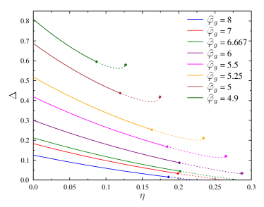
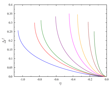
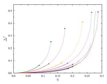
Figure 4: $\Delta$ (top panels) and $\Delta^{f}$ (bottom panels), solutions of Eqs. (72)-(73), for different glassy states followed in decompression ($\eta<0$, left panels) and compression ($\eta>0$, right panels). We use separate scales to improve the readability of the figures. The dashed lines indicate the unstable region where the replicon mode is positive (Fig. 5).

In Fig. (4) we report the evolution of $\Delta$ and $\Delta^{f}$ under compression ($\eta>0$) or decompression ($\eta<0$) at $\gamma=0$. The corresponding pressure is reported in Fig.1 of the main text. In decompression, we find that $\Delta^{f}$ increases quadratically from zero, while $\Delta$ also increases. At low enough $\eta$, a spinodal point is met, where the solution disappears. This is signaled by a square-root singularity in both $\Delta$ and $\Delta^{f}$, as usual for spinodal points. At that point the glass ceases to exist and melts into the liquid phase.

In compression, again $\Delta^{f}$ increases quadratically while $\Delta$ decreases. At high enough $\widehat{\varphi}_{g}$ (see e.g. $\widehat{\varphi}_{g}=8$ in Fig. 4), $\Delta$ vanishes linearly at $\eta_{j}$, while $\Delta^{f}$ is finite at $\eta_{j}$, as predicted by the asymptotic analysis of Sec. C.3. The values of $\eta_{j}$ and $\Delta^{f}_{j}$ coincide with the ones obtained using the analysis of Sec. C.3. At low density (see e.g. $\widehat{\varphi}_{g}=5$ in Fig. 4), however, before the jamming point, an unphysical spinodal point is reached (signaled again by a square root singularity), marked by a symbol in Fig. 4. This unphysical spinodal point has also been found in spin glasses Zdeborová and Krzakala (2010).

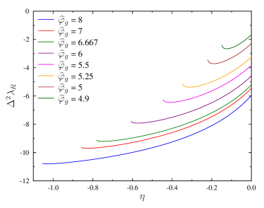
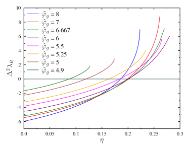
Figure 5: The replicon mode given by Eq. (70), for the same glasses as in Fig. 4 and Fig.1 of the main text. In decompression the replicon is always negative, therefore the RS solution is stable; in compression, the replicon vanishes at the Gardner transition signaling an instability of the RS solution.

In both cases, before either jamming or the unphysical spinodal point is reached, the replicon mode becomes positive (Fig. 5), signaling that the glass state undergoes a Gardner transition Gardner (1985); Charbonneau et al. (2014b) and beyond that point the RS solution we used is not correct. Based on the analogy with spin glasses and in particular on the results of Zdeborová and Krzakala (2010), and on the discussion of Sec. A.6.1, we expect that at the Gardner transition replica symmetry is broken towards a fullRSB solution. A 1RSB structure in the $s$-block should already give an excellent approximation of the equation of state of the glass and eliminate the unphysical spinodal point. We leave this computation for future work. The unstable part of the curves in Fig. 4 is reported with dashed lines.

The result for shear modulus, reported in Fig.3 of the main text, is easily deduced from the results for $\Delta$ reported in Fig. 4 using Eq. (79). We can also compute the dilatancy from Eq. (82): the result is reported in Fig. 6. Note that $R/\rho=(1/2)\widehat{\varphi}\partial\mu/\partial\widehat{\varphi}$ as it can be deduced by combining Eqs. (82) and (79). From Eq. (82) it is also clear that $R$ diverges at the spinodal point where $\Delta$ has a square-root singularity (hence infinite derivative) and at the jamming point where $\Delta\rightarrow 0$.

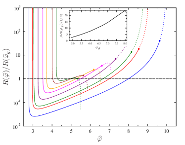
Figure 6: Dilatancy $R$ as a function of density for different glasses. Colors and styles as in Fig. 3 of the main text where the shear modulus $\mu$ is reported. Recall that $R/\rho=(1/2)\widehat{\varphi}\partial\mu/\partial\widehat{\varphi}$. In the inset, the evolutions of $R(\widehat{\varphi}_{g})$ with $\widehat{\varphi}_{g}$ is reported. Note that the dilatancy diverges both at jamming and at the low density spinodal point where the glass melts.

D.2 Shear

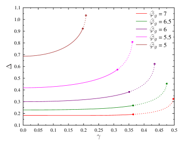
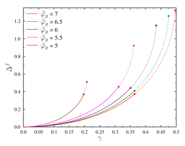
Figure 7: Values of $\Delta$ (left panel) and $\Delta^{f}$ (right panel) as functions of shear strain $\gamma$ in absence of compression ($\eta=0$). The dashed lines indicate the unstable region where the replicon mode is positive (Fig. 8).

We next analyze the behavior under a shear strain $\gamma$ in absence of compression, hence for $\eta=0$. The results for $\Delta$ and $\Delta^{f}$ are reported in Fig. 7. We observe that upon increasing $\gamma$ both $\Delta$ and $\Delta^{f}$ increase, until a spinodal point is reached, at which they both display a square root singularity. Correspondingly, both the shear stress $\sigma$ and the glass pressure $p_{g}$ (main text, Fig.2) display a square root singularity.

However, before the spinodal is met, the replicon mode becomes positive (Fig. 8) and the system undergoes a Gardner transition. The fact that the a Gardner transition is met when the system is subject to a shear strain might be surprising at first sight, because one could think that straining a well defined glass basin amounts to deform the basins but should not induce its breaking into sub-basins. However, note first that on general grounds, the free energy landscape can change once perturbations are added. Moreover, we find (see Fig.2 in the main text) that the pressure of the glassy state increases when the shear strain is increased. This means that under shear strain the particles in the glass basins become more constrained and because of this some parts of the basin can become forbidden, triggering the Gardner transition as it happens during a compression in absence of shear strain.

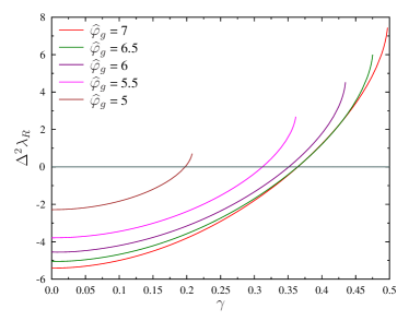
Figure 8: The replicon mode given by Eq. (70), for the same glasses as in Fig. 7 and Fig.2 of the main text. The replicon vanishes at the Gardner transition signaling an instability of the RS solution.

D.3 Quality of the approximation $\Delta^{f}=0$

To conclude, we comment on the quality of the approximation $\Delta^{f}$ discussed in Sec. C.4 at $\gamma=0$. We see from the results of Fig. 4 that this approximation is reasonable, except close to the spinodals where $\Delta^{f}$ grows rapidly. Correspondingly, we find that the approximation $\Delta^{f}=0$ misses the spinodals. In decompression, the states can be followed to arbitrarily low density, which is clearly unphysical. In compression, the spinodal is missed, but the Gardner transition is predicted with quite good accuracy, hence the approximation does a fair job in the physical region.

Appendix E Comparison with previous work

Let us conclude by a comparison with previous work Parisi and Zamponi (2010); Kurchan et al. (2012, 2013); Charbonneau et al. (2014b), in which the Monasson formalism was used Monasson (1995). Let us illustrate shortly the outcome of the Monasson computation. We restrict to hard spheres for simplicity. At a given packing fraction $\varphi$ in the glass phase, the phase space of the system is decomposed in a certain number of glassy states, each glass state being a cluster of configurations (for an analysis of this clustering phenomenon in a similar context see Krzakala et al. (2007)). Each cluster contains a certain number of configurations, which defines its internal entropy $s$. The complexity $\Sigma(s)=N^{-1}\log{\cal N}(s)$ is the logarithm of the number of clusters that have entropy $s$, at fixed density $\varphi$. This is what is computed by the Monasson formalism (through the introduction of a parameter $m$ conjugated to the internal entropy of the cluster). The crucial point, however, is the following. Consider all the clusters with total entropy $s$. Among them, there are clusters with different properties (e.g. pressure, shear modulus, etc.). However, since the total number of clusters is exponential in $N$, as usual in statistical mechanics, there is a subset of them (we call them typical) that have typical properties (same pressure, same shear modulus, etc.). The Monasson formalism allows one to compute the properties of these typical states. Hence, the resulting pressure-density phase diagram reported in Parisi and Zamponi (2010); Charbonneau et al. (2014b) refers to the properties of the typical states.

On the other hand, it is well known in spin glasses Mézard et al. (1987) that if one takes some states that are typical at a given state point (i.e. at a given density and internal entropy, or equivalently, at a given density and pressure) and follows their evolution at a different state point (e.g. at a different density), they become atypical. This means that they have in general different values of thermodynamic observables with respect to the typical states at the new state point. The Franz-Parisi formalism Franz and Parisi (1995); Barrat et al. (1997) (or “state following” formalism Zdeborová and Krzakala (2010); Krzakala and Zdeborová (2013) allows one to select a typical glass state in some state point, and follow its evolution to a different state point. In this paper we have focused on states that are typical at a given density $\varphi_{g}$ and at the value of pressure corresponding to the equilibrium liquid pressure at density $\varphi_{g}$ (that for infinite-dimensional hard spheres is just $p/d=\widehat{\varphi}_{g}/2$), and we followed their evolution in compression and in shear. In the Monasson formalism, these states are selected by choosing $m=1$. Choosing different values of $m$ (here we wrote all the equations for general $m$ even if in the end we only considered $m=1$) allows one to select different states, and then we can follow them to a different state point using the formalism we developed above.

The most interesting and striking difference with respect to the typical computation Kurchan et al. (2013); Charbonneau et al. (2014b) (see also Rizzo (2013) for spin glasses) concerns the behavior of the Gardner transition line (main text, Fig.1) around the dynamical transition. In the present work, we showed that for states prepared at $\varphi_{g}=\varphi_{\rm d}$, the Gardner transition is met immediately after an infinitesimal compression (see also Barrat et al. (1997); Franz et al. ). In other words, the Gardner transition line ends at the dynamical transition (see main text, Fig.1). This can be understood heuristically by observing that glasses with $\varphi_{g}\sim\varphi_{\rm d}$ correspond to fast compression procedures, while glassy states with $\varphi_{g}\gg\varphi_{\rm d}$ correspond to very slow compression. It is therefore reasonable that the former are more unstable than the latter. However, in Rizzo (2013); Kurchan et al. (2013) it was found that the fullRSB phase appears only above a given packing fraction $\varphi^{*}>\varphi_{d}$ implying that all states around the dynamical point are stable and no fullRSB is present around $\varphi_{\rm d}$. The reason behind this difference is that the equilibrium states, once followed in different state points, become immediately atypical. The states prepared at $\varphi_{\rm d}$ undergo a Gardner transition immediately under compression, but they become atypical and are not detected by the Monasson computation Kurchan et al. (2013), which find instead other glassy states that appear away from equilibrium and are stable until $\varphi<\varphi^{*}$. This is a signal that the evolution of the free energy landscape under external perturbations is very chaotic in the region around $\varphi_{\rm d}$.

References

- Cavagna (2009) A. Cavagna, Physics Reports 476, 51 (2009).
- Dyre (2006) J. C. Dyre, Rev.Mod.Phys. 78, 953 (2006).
- Swallen et al. (2007) S. F. Swallen, K. L. Kearns, M. K. Mapes, Y. S. Kim, R. J. McMahon, M. D. Ediger, T. Wu, L. Yu, and S. Satija, Science 315, 353 (2007).
- Singh et al. (2013) S. Singh, M. Ediger, and J. J. de Pablo, Nature Materials 12, 139 (2013).
- Rodney et al. (2011) D. Rodney, A. Tanguy, and D. Vandembroucq, Modelling and Simulation in Materials Science and Engineering 19, 083001 (2011).
- Koumakis et al. (2012) N. Koumakis, M. Laurati, S. U. Egelhaaf, J. F. Brady, and G. Petekidis, Phys.Rev.Lett. 108, 098303 (2012).
- Götze (2009) W. Götze, Complex dynamics of glass-forming liquids: A mode-coupling theory, vol. 143 (OUP, USA, 2009).
- Brader et al. (2009) J. M. Brader, T. Voigtmann, M. Fuchs, R. G. Larson, and M. E. Cates, PNAS 106, 15186 (2009).
- Ikeda and Berthier (2013) A. Ikeda and L. Berthier, Phys. Rev. E 88, 052305 (2013).
- Keys et al. (2013) A. S. Keys, J. P. Garrahan, and D. Chandler, PNAS 110, 4482 (2013).
- Penrose and Lebowitz (1971) O. Penrose and J. L. Lebowitz, Journal of Statistical Physics 3, 211 (1971).
- Langer (1974) J. S. Langer, Physica 73, 61 (1974).
- Kirkpatrick and Wolynes (1987) T. R. Kirkpatrick and P. G. Wolynes, Phys. Rev. A 35, 3072 (1987).
- Kirkpatrick and Thirumalai (1989) T. R. Kirkpatrick and D. Thirumalai, Journal of Physics A: Mathematical and General 22, L149 (1989).
- Monasson (1995) R. Monasson, Phys. Rev. Lett. 75, 2847 (1995).
- Franz and Parisi (1995) S. Franz and G. Parisi, Journal de Physique I 5, 1401 (1995).
- Barrat et al. (1997) A. Barrat, S. Franz, and G. Parisi, Journal of Physics A: Mathematical and General 30, 5593 (1997).
- Zdeborová and Krzakala (2010) L. Zdeborová and F. Krzakala, Phys. Rev. B 81, 224205 (2010).
- Krzakala and Zdeborová (2013) F. Krzakala and L. Zdeborová, Journal of Physics: Conference Series 473, 12022 (2013).
- Parisi and Zamponi (2010) G. Parisi and F. Zamponi, Rev. Mod. Phys. 82, 789 (2010).
- Charbonneau et al. (2014a) P. Charbonneau, J. Kurchan, G. Parisi, P. Urbani, and F. Zamponi, Nature Communications 5, 3725 (2014a).
- Mezard and Parisi (2012) M. Mezard and G. Parisi, in Structural Glasses and Supercooled Liquids: Theory, Experiment and Applications, edited by P.G.Wolynes and V.Lubchenko (Wiley & Sons, 2012), eprint arXiv:0910.2838.
- (23) S. Franz, G. Parisi, and F. Ricci-Tersenghi, to appear.
- Charbonneau et al. (2011) P. Charbonneau, A. Ikeda, G. Parisi, and F. Zamponi, Phys. Rev. Lett. 107, 185702 (2011).
- Gardner (1985) E. Gardner, Nuclear Physics B 257, 747 (1985).
- (26) M. Mariani, G. Parisi, and C. Rainone, to appear.
- Tighe (2014) B. P. Tighe, Granular Matter 16, 203 (2014).
- Yoshino and Zamponi (2014) H. Yoshino and F. Zamponi, Phys. Rev. E 90, 022302 (2014).
- Ren et al. (2013) J. Ren, J. A. Dijksman, and R. P. Behringer, Phys.Rev.Lett. 110, 018302 (2013).
- Coulais et al. (2014) C. Coulais, A. Seguin, and O. Dauchot, arXiv:1403.5885 (2014).
- Otsuki and Hayakawa (2014) M. Otsuki and H. Hayakawa, Phys. Rev. E 90, 042202 (2014).
- Berthier et al. (2011) L. Berthier, H. Jacquin, and F. Zamponi, Phys. Rev. E 84, 051103 (2011).
- Kurchan et al. (2012) J. Kurchan, G. Parisi, and F. Zamponi, JSTAT 2012, P10012 (2012).
- Kurchan et al. (2013) J. Kurchan, G. Parisi, P. Urbani, and F. Zamponi, J. Phys. Chem. B 117, 12979 (2013).
- Charbonneau et al. (2014b) P. Charbonneau, J. Kurchan, G. Parisi, P. Urbani, and F. Zamponi, JSTAT 2014, P10009 (2014b).
- Mézard and Parisi (2000) M. Mézard and G. Parisi, Journal of Physics: Condensed Matter 12, 6655 (2000).
- Mézard and Parisi (1999) M. Mézard and G. Parisi, The Journal of Chemical Physics 111, 1076 (1999).
- Lubachevsky and Stillinger (1990) B. D. Lubachevsky and F. H. Stillinger, J. Stat. Phys. 60, 561 (1990).
- Yoshino and Mézard (2010) H. Yoshino and M. Mézard, Phys. Rev. Lett. 105, 015504 (2010).
- Yoshino (2012) H. Yoshino, The Journal of Chemical Physics 136, 214108 (2012).
- Rizzo (2013) T. Rizzo, Phys. Rev. E 88, 032135 (2013).
- Mézard et al. (1987) M. Mézard, G. Parisi, and M. A. Virasoro, Spin glass theory and beyond (World Scientific, Singapore, 1987).
- Hansen and McDonald (1986) J.-P. Hansen and I. R. McDonald, Theory of simple liquids (Academic Press, London, 1986).
- Krzakala et al. (2007) F. Krzakala, A. Montanari, F. Ricci-Tersenghi, G. Semerjian, and L. Zdeborova, Proceedings of the National Academy of Sciences 104, 10318 (2007).