Finding Hot-Jupiters by Gaia photometry using the Directed Follow-Up strategy

Abstract

All-sky surveys of low-cadence nature, such as the promising Gaia Space mission, have the potential to ”hide” planetary transit signals. We developed a novel detection technique, the Directed Follow-Up strategy (DFU), to search for transiting planets using sparse, low-cadence data. According to our analysis, the expected yield of transiting Hot-Jupiters that can be revealed by Gaia will reach a few thousands, if the DFU strategy will be applied to facilitate detection of transiting planets with ground-based observations. This will guaranty that Gaia will exploit its photometric capabilities and will have a strong impact on the field of transiting planets, and in particular on detection of Hot-Jupiters. Besides transiting exoplanets Gaia’s yield is expected to include a few tens of transiting brown dwarfs, that will be candidates for detailed characterization, thus will help to bridge the gap between giant planets and stars.

1 Introduction

Transiting planets, in particular Hot-Jupiters (HJs) orbiting bright stars, are of the most appealing objects to detect, since they are favorable for observational follow-up study. As such, they are keys for studying the mechanism that drive planetary formation, migration and evolution. The Directed Follow-Up strategy (DFU) is a detection approach that we use to search for transiting HJs in sparse, low-cadence data, such as Hipparcos (ESA, 1997), and its successor Gaia (de Bruijne, 2012). Several studies examined the feasibility of detecting transits in the Hipparcos Epoch Photometry, and made posterior detections of two known transiting planets in Hipparcos, using the previously available knowledge of the orbital elements of the exoplanets (e.g., Robichon & Arenou, 2000; Bouchy et al., 2005). Those studies concluded that Hipparcos was not sufficient for transit detection, without using prior information (Hébrard & Lecavelier Des Etangs, 2006). The posterior detections prove that the information about the transits is buried in the data, and that motivated us to look for a way to utilize low-cadence photometric surveys for transit search.

2 Directed Follow-Up strategy for low-cadence surveys

The DFU strategy is based on Bayesian inference that we use to estimate the posterior probability density functions of the transit parameters. We describe the transit by a simple box-shaped light-curve (.e.g, Kovács et al., 2002) with five parameters: the period – $P$, phase – $T_{c}$, and width of the transit – $w$, and the flux levels in and out of transit.

First we apply a Metropolis-Hastings (MH) algorithm (implementation of a Markov-Chain Monte-Carlo procedure) to the measurements of a target star. The results (after excluding the appropriate ‘burning time’) are Markov chains of the successful iterations, for each of the model parameters. From each chain we extract the stationary distribution, which we use as the parameter’s estimated Bayesian posterior distribution (Gregory, 2005). If the low-cadence data happen to sample enough separate transits, with sufficient precision, we expect the distributions to concentrate around the solution of the transit. But unlike the case of precise high-cadence surveys, even if the star hosts a transiting planet, due to the low-cadence observations, only a few transits will be sampled. Therefore, the distributions will probably spread over different solutions, besides the unknown actual one.

The second step is to assign probability for a transit for future times, which is represented by the Instantaneous Transit Probability function (ITP). Then we will choose stars for a follow-up campaign according to the ITP peak values and skewness, both are indications for the presence (or absence) of a periodic transit-like signal in the data. Another criterion is the Wald statistic of the transit depth posterior distribution, that quantifies the significance of the transit depth by measuring it in terms of its own standard deviation.

The last step is to actually perform follow-up observations, at the times directed by the ITP, thus optimizing the chances to detect the transit in a few observations as possible. Then the follow-up observations should be combined with the data from the survey, to recalculate new posterior distributions that reflect our new state of knowledge, and to propose new times for the next follow-up observations.

If a follow-up observation happens to take place during transit, it will usually eliminate most spurious peaks in the period posterior distribution (PPD), except for the actual orbital period of the planet. However, usually we will not observe the transit in the follow-up observations. In this case the new data will still eliminate some periods that will not fit our new state of knowledge, resulting in modified posterior distributions of the model parameters. The whole procedure should be repeated until the detection of a transiting planet, or, alternatively the exclusion of its existence. After we will detect a planetary candidate a careful high-cadence photometric or spectroscopic follow-up can confirm its planetary nature.

3 DFU application to Gaia

Gaia was initially intended to detect exoplanets using its unprecedented astrometry, and in this aspect it will have an innovative contribution to planetary research (see e.g., Lattanzi & Sozzetti, 2010; Sozzetti, 2013, 2014). In Dzigan & Zucker (2012) we showed that despite the non-competitive photometry of the telescope (relative to dedicated transit surveys), Gaia will be useful for transit search. In Dzigan & Zucker (2013) we demonstrated the application of the strategy to Gaia using a few simulated cases,and advocate for the use of real-time follow-up resources as means to identify transiting planets, to begin during the operational lifetime of the mission.

3.1 Gaia’s expected yield of transiting exoplanets

To estimate Gaia’s expected yield of transiting exoplanets, we followed a statistical methodology (Beatty & Gaudi, 2008) that accounts for the transit probability, transiting planet frequencies based on complete transit surveys (namely OGLE), and assumptions regarding the galactic structure. We found that the potential yield can reach a few thousands, depending on the number of planetary transits that the telescope should sample to secure detection, and therefore on the detection algorithm (Dzigan & Zucker, 2012). The observational window functions (von Braun et al., 2009) in Fig. 1 represent the probability to sample a minimum of three, five and seven transits for a typical Gaia star, with $70$ measurements (upper panel), together with another, less probable case, with $197$ measurements (bottom panel). For a typical Gaia star that hosts a transiting HJ (upper panel of Fig. 1), the probability to sample at least seven separate transits is practically negligible. The probability to sample five transits is $\sim 5\%$, while the probability to sample a minimum of three transits increases to $\sim 30\%$. Thus, we conclude that it will be beneficial to relax the requirement for a minimum number of sampled transits that can secure a detection, and the DFU strategy aims to achieve exactly that. It is worth nothing that for stars located at ecliptic latitudes of $\pm 45$ deg, the probability to sample at least three different transits amount to almost $100\%$ (bottom panel of Fig. 1).

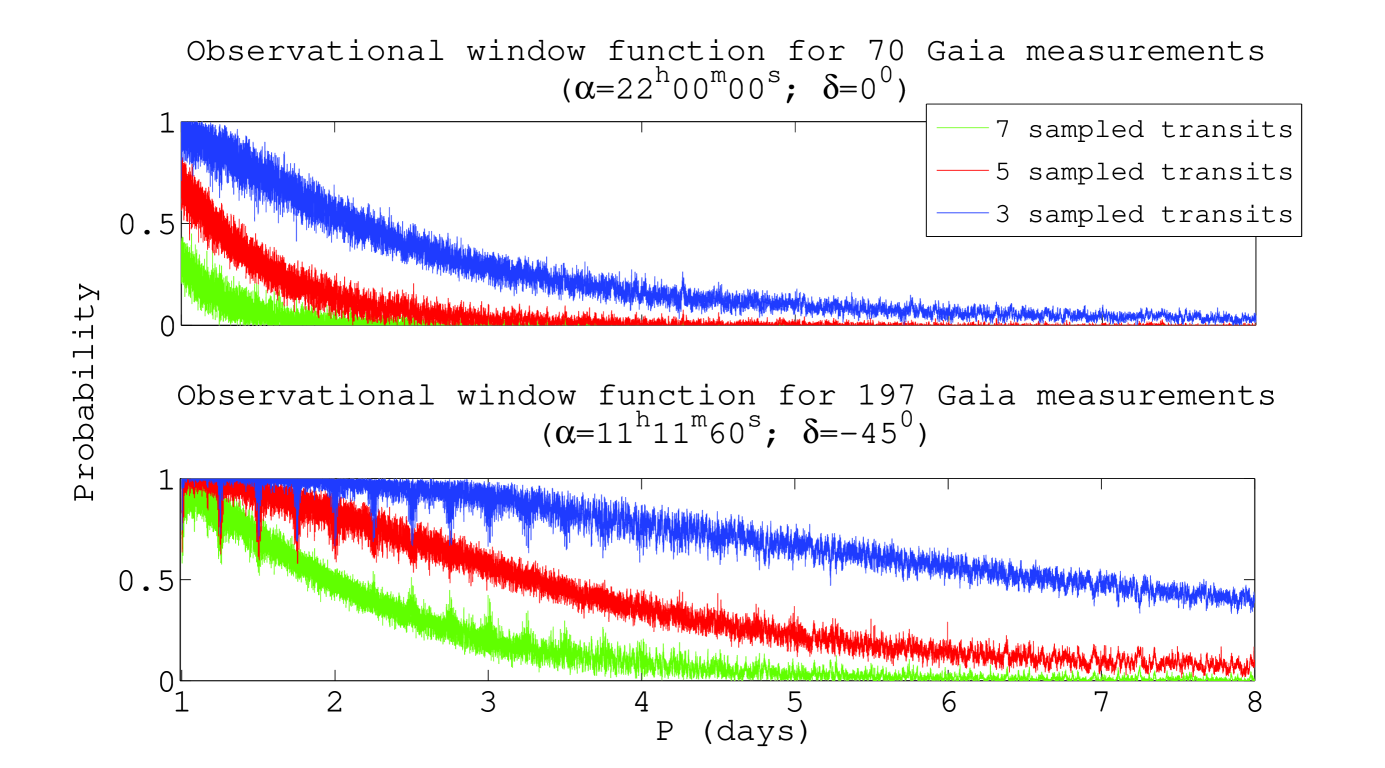
Figure 1: Observational window functions for two areas of Gaia’s sky, as discussed in Dzigan & Zucker (2013). Top: A sky direction that Gaia is expected to visit $70$ times. Bottom: A sky direction that Gaia is expected to sample $197$ times. Both window functions were calculated for a transit duration of $2\,\mathrm{hr}$, for a minimum of three, five and seven in-transit observations.

3.2 application to Gaia

We examined the application of the strategy to Gaia using a few simulated cases, inspired by known transiting planets. We simulated light curves of planetary transits according to Gaia’s scanning-law and expected photometric precision (Dzigan & Zucker, 2013). Each planet was assigned with a transit epoch that implied different number of transit samples. We found that DFU can result in detection through one of two main scenarios. The first scenario is a detection using Gaia data alone. In this scenario the MH algorithm culminates in a PPD that is centered around a single solution, (and maybe its harmonics and sub-harmonics). The compact distribution will guarantee that the resulting ITP peaks will coincide with future transits. Therefore we will be able to direct a high cadence follow-up observations, to examine the nature of the candidate. We found that in case Gaia will sample five different transits pwe system, the strategy will result in a detection using Gaia data alone (an example can be found in Dzigan & Zucker (2013)).

Due to Gaia’s low cadence, in most cases we expect to obtain multimodal PPD (Dzigan & Zucker, 2011). This will result in the second scenario, in which we will require more than a single follow-up observation in order to finally detect the transit.

We demonstrate the strategy application for Gaia in Fig. 2, using a simulation inspired by WASP-4b. We tailored the transit phase, so that Gaia’s scanning-law will sample four individual transits during the complete mission lifetime (five nominal years). For a relatively small transit depth (five mmag) the strategy yield a detection using two directed follow-up observations. We found that with as little as three transits samples, we would be able to trigger follow-up observations that will eventually lead to the transit detection (using two or more follow-up sequences).

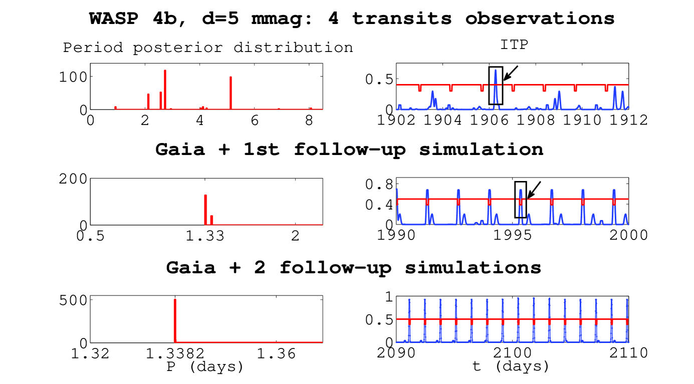
Figure 2: Application of the DFU strategy for Gaia simulation, as discussed in Dzigan & Zucker (2013). Top: PPD and ITP for a simulation inspired by WASP-4b, $d=5\,\mathrm{mmag}$, 4 sampled transits. Middle: PPD and ITP for the combined datasets (adding the first follow-up observing sequence, simulated according to the marked ITP peak, not during transit.) Bottom: New PPD and ITP after adding the second follow-up sequence, which was simulated according to the marked ITP peak that this time did sample the hypothetical transit.

3.3 Alerts for follow-up observations during Gaia operation

Due to the ITP degradation (Dzigan & Zucker, 2011), we suggest that the follow-up campaign will begin as soon as possible, while Gaia still operates. In Dzigan & Zucker (2013) we examined simulations using half of Gaia’s timespan, and found it will be possible to trigger follow-up observations if Gaia will sample three transits in this short time interval (at least two years of data).

The DFU strategy requires a widely spread network, able to follow-up on prominent ITP peaks during the mission lifetime. Gaia Science Alerts team (Wyrzykowski & Hodgkin, 2012) is assigned to trigger follow-up observations for transient events in the Gaia data stream. Although planetary transits are not transient, the information about the transit is, so Science Alerts may prove as beneficial for the strategy implementation.

4 Discussion and Summary

We introduced the DFU strategy, and examined its application to Gaia photometry. We found that for all simulated light curves with transits deeper than $1\,\mathrm{mmag}$, the DFU strategy can be used to either recover the periodicity, or to propose times for directed follow-up observations that will lead to detection. If a typical HJ ($d\sim 10\,\mathrm{mmag}$), will be sampled by Gaia during five different transits, a detection will be possible using Gaia data alone. A more realistic scenario, with only three in-transit measurements, will usually result in a detection under a follow-up campaign, based on the ITP most significant peaks, that will reduce the observational efforts to a minimum. Test light curves with no transit signal were never classified as candidates, and were not prioritized for follow-up observations.

We showed (Dzigan & Zucker, 2012) that the false-alarm rate due to Gaia’s white Gaussian noise is negligible, and that our prioritization procedure eliminated all the false alarms that resulted from stellar red noise (Dzigan & Zucker, 2013).

In Dzigan & Zucker (2012) we studied the yield of transiting planets from Gaia, and predict that the yield can reach a few thousands, provided that the detection algorithm will be tailored for Gaia’s special features.

Since our ability to schedule follow-up observations based on the ITP degrades with time, the optimal scenario for Gaia will be to initiate the follow-up campaign while Gaia still operates. Simulating only two to three years of Gaia observations, we found that we will be able to prioritize stars and trigger follow-up observations using partial data (Dzigan & Zucker, 2013). As indicated by the window function in Fig. 1, stars located close to the knots of the scanning-law will be sampled during different transits more quickly, thus allowing the follow-up to begin even earlier.

In addition to transiting HJs, Gaia is expected to yield a few tens of transiting brown dwarfs (Bouchy, 2014), that can be studied in details using follow-up observations, and will help to bridge the gap between giant planets and stars.

We conclude that Gaia photometry, although not optimized for transit detection, should not be ignored in the search of transiting planets. A timely application of the DFU strategy will eventually yield the detection of thousands of transiting HJs, and will promise that Gaia will contribute to the photometric search of planets via transits, along with its anticipated astrometric detections.