Hydrodynamics in graphene: Linear-response transport

B.N. Narozhny Institut für Theorie der Kondensierten Materie, Karlsruher Institut für Technologie, 76128 Karlsruhe, Germany National Research Nuclear University MEPhI (Moscow Engineering Physics Institute), Kashirskoe shosse 31, 115409 Moscow, Russia    I.V. Gornyi Institut für Nanotechnologie, Karlsruhe Institute of Technology, 76021 Karlsruhe, Germany A.F. Ioffe Physico-Technical Institute, 194021 St. Petersburg, Russia    M. Titov Radboud University Nijmegen, Institute for Molecules and Materials, NL-6525 AJ Nijmegen, The Netherlands    M. Schütt School of Physics and Astronomy, University of Minnesota, Minneapolis, MN 55455, USA    A.D. Mirlin Institut für Nanotechnologie, Karlsruhe Institute of Technology, 76021 Karlsruhe, Germany Institut für Theorie der Kondensierten Materie, Karlsruher Institut für Technologie, 76128 Karlsruhe, Germany Petersburg Nuclear Physics Institute, 188350 St. Petersburg, Russia
Abstract

We develop a hydrodynamic description of transport properties in graphene-based systems which we derive from the quantum kinetic equation. In the interaction-dominated regime, the collinear scattering singularity in the collision integral leads to fast unidirectional thermalization and allows us to describe the system in terms of three macroscopic currents carrying electric charge, energy, and quasiparticle imbalance. Within this “three-mode” approximation we evaluate transport coefficients in monolayer graphene as well as in double-layer graphene-based structures. The resulting classical magnetoresistance is strongly sensitive to the interplay between the sample geometry and leading relaxation processes. In small, mesoscopic samples the macroscopic currents are inhomogeneous which leads to linear magnetoresistance in classically strong fields. Applying our theory to double-layer graphene-based systems, we provide microscopic foundation for phenomenological description of giant magnetodrag at charge neutrality and find magnetodrag and Hall drag in doped graphene.

pacs:
72.80.Vp, 73.23.Ad, 73.63.Bd

Traditional hydrodynamics dau describes systems at large length scales (compared to the mean free path). The hydrodynamic equations are typically formulated in terms of currents and densities of conserved quantities and can be derived from the kinetic equation using either the Chapman-Enskog cen or Grad gra procedures. Within the leading approximation, gradients of the macroscopic physical quantities are assumed to be small, such that the system can be characterized by the local equilibrium distribution function. Dissipative properties, such as electrical or thermal conductivity or viscosity are then determined by small corrections to the local-equilibrium distribution function. Within linear response, such corrections are proportional to a weak external bias.

Recently the kinetic equation approach was applied to electronic excitations in graphene kas ; mu1 ; mu2 ; kin ; fos ; ryz ; mem . In contrast to conventional metals and semiconductors, graphene is characterized by the linear excitation spectrum which makes the system explicitly non-Galilean-invariant. Consequently, the transport scattering time in graphene is strongly affected by electron-electron interaction pol which has to be taken into account on equal footing with disorder potential. At the same time, due to the classical nature of the Coulomb interaction between charge carriers in graphene, the system is also non-Lorentz-invariant. As a result, the standard derivation dau of the hydrodynamic equations from the kinetic equation has to be revisited kas ; mu1 ; mu2 ; kin ; fos ; ryz ; mem .

The linearity of the quasiparticle spectrum in graphene leads to an important corollary: the energy and momentum conservation laws for Dirac quasiparticles coincide in the special case of collinear scattering. This kinematic peculiarity results in a singular contribution to the collision integral kas ; mu1 ; kin ; mem allowing for a non-perturbative solution to the kinetic equation. The distinct feature of this solution is fast unidirectional thermalization mem that facilitates integration of the kinetic equation. The unique feature of the resulting hydrodynamic description of electronic transport in graphene is inequivalence of the electric current and total momentum of the system mu1 ; mu2 ; mem . As the latter is equivalent to the energy current, transport properties of graphene are governed by a non-trivial interplay of electric current and energy relaxation.

Two-fluid hydrodynamics in graphene was suggested in Refs. mu1, ; fos, and then extended to double-layer graphene-based structures in Ref. mem, , which allowed for a description of the Coulomb drag effect gor ; tu1 ; tu2 ; meg in graphene. An extension of this approach to mesoscopic (finite-size) samples was suggested in Ref. meg, . Qualitatively, this theory can be interpreted in terms of a semiclassical two-band model that yields non-trivial magnetic field dependence of the transport coefficients and accounts for the effect of giant magnetodrag at the neutrality point meg . The classical mechanism of this effect is similar to the standard mechanism of magnetoresistance in multi-band systems bsm .

In this paper we rigorously derive the hydrodynamic description of electronic transport in graphene within linear response. While we use the same collinear-scattering singularity as found in Refs. kas, ; mu1, ; kin, ; mem, in order to integrate the quantum kinetic equation, we argue that the physics of the system should be described in terms of three macroscopic currents: the electric current $\boldsymbol{j}$, energy current $\boldsymbol{Q}$, and quasiparticle imbalance fos current $\boldsymbol{P}$.

For general doping, the resulting theory is rather cumbersome. However, at the charge neutrality point and in the degenerate limit the equations simplify allowing for an analytic solution. In the former case, we focus on the issue of magnetoresistance, a subject of considerable experimental interest fu1 ; fu2 ; job ; mg1 ; mg2 ; mg3 ; mg4 . In particular, we demonstrate the appearance of the linear magnetoresistance in moderately strong, classical magnetic fields in monolayer graphene mrs . In double-layer graphene-based systems we describe negative Coulomb drag meg ; lev and justify the phenomenological two-band model of Ref. meg, (precisely at the Dirac point the imbalance current is proportional to the energy current allowing one to reduce the number of variables). Both effects occur in narrow, mesoscopic samples in the presence of energy relaxation and quasiparticle recombination due to electron-phonon interaction.

In the opposite limit of very high doping (i.e. in the “Fermi-liquid regime”) all three macroscopic currents become equivalent and the theory is reduced to the standard Drude-like description that can be also derived by perturbative methods us1 . Here we find the leading corrections to the standard picture of Coulomb drag us1 ; thd yielding magnetodrag and Hall drag in doped graphene.

The rest of the paper is organized as follows. We begin (Section I) with the summary of our theory and results for monolayer graphene. In Section II, we present a derivation of the macroscopic description of electronic transport. In Section III, we use this theory to evaluate transport coefficients in graphene such as the magnetoresistance at the point of charge neutrality for small, mesoscopic samples. In Section IV, we apply our theory to double-layer graphene-based systems gor ; tu1 ; tu2 ; meg . Concluding remarks can be found in Section V. Technical details are relegated to the Appendices.

I Macroscopic description of transport in monolayer graphene

In this Section, we describe transport properties of monolayer graphene. Neglecting all quantum effects aar ; zna ; fal , we base our considerations on the set of macroscopic transport equations which essentially generalize the usual Ohm’s law to the case of collision-dominated transport in graphene. These equations can be derived from the kinetic equation (see Section II below) in the interaction-dominated regime, where the transport scattering time due to electron-electron interaction $\tau_{ee}$ is much smaller than the disorder mean-free time $\tau$

$$\tau_{ee}\ll\tau.$$

We limit ourselves to the discussion of a steady state. The latter is typically established by means of disorder scattering. A notable exception is neutral graphene in the absence of magnetic field, where the steady state exist due to electron-electron interaction alone. However, in the presence of the field, even at the Dirac point the steady state cannot be reached without disorder. Therefore, we have to keep the weak disorder in the problem. For simplicity, we assume the mean-free time $\tau$ to be energy independent, although in physical graphene most of the impurity scattering processes lead to energy-dependent relaxation rates. A corresponding generalization of our theory is straightforward us1 and does not lead to qualitatively new effects fn1 . At the same time, quantitative description of experimental data may greatly benefit from a realistic description of disorder meg .

Non-linear hydrodynamics of graphene will be discussed in a separate publication ulf .

I.1 Linear response equations in graphene

One of the main results of this paper is the set of macroscopic equations describing electronic transport in graphene within linear response. What makes this unusual is that the electric current $\boldsymbol{j}$ is inequivalent to the energy current $\boldsymbol{Q}$ and the quasiparticle imbalance current $\boldsymbol{P}$. The three macroscopic currents can be found from the following equations

$$-\boldsymbol{\nabla}\Pi+\boldsymbol{E}+{\cal R}_{H}\boldsymbol{\cal K}\times\boldsymbol{e}_{\boldsymbol{B}}={\cal R}_{0}\boldsymbol{j}+\frac{\pi}{e^{2}K}\left[\frac{\boldsymbol{\cal A}}{\tau_{vv}}+\frac{\boldsymbol{\cal C}}{\tau_{vs}}\right],$$ (1a)
$\displaystyle-\boldsymbol{\nabla}\Theta+{\cal N}_{1}\boldsymbol{E}+{\cal R}_{H}\left[\boldsymbol{j}\times\boldsymbol{e}_{\boldsymbol{B}}\right]={\cal R}_{0}\frac{e}{K}\boldsymbol{Q},$ (1b)
$$-\boldsymbol{\nabla}\Xi+\frac{\mu}{K}\boldsymbol{E}+{\cal R}_{H}\widetilde{\boldsymbol{\cal K}}\times\boldsymbol{e}_{\boldsymbol{B}}=e{\cal R}_{0}\boldsymbol{P}+\frac{\pi}{e^{2}K}\left[\frac{\boldsymbol{\cal A}}{\tau_{vs}}+\frac{\boldsymbol{\cal C}}{\tau_{ss}}\right].$$ (1c)

Here $\boldsymbol{E}$ is the electric field, $\boldsymbol{e}_{\boldsymbol{B}}$ is the unit vector in the direction of the magnetic field $\boldsymbol{B}=B\boldsymbol{e}_{\boldsymbol{B}}$, $K$ is the mean quasiparticle kinetic energy in graphene meg (with $T$ being the temperature and $\mu$ the chemical potential):

$$K=2T\ln\left(1+e^{\mu/T}\right)-\mu\rightarrow\left\{\begin{matrix}\mu&,&T\ll\mu\cr 2T\ln 2&,&T\gg\mu\end{matrix}\right.,$$ (2)

the dimensionless quantity ${{\cal N}_{1}=2n_{0}/(\nu_{0}K)}$ represents the equilibrium charge density $n_{0}$ (here $\nu_{0}=\partial n_{0}/\partial\mu$), and the two coefficients ${\cal R}_{0}$ and ${\cal R}_{H}$ are

$${\cal R}_{0}(\mu,\tau,T)=\frac{\pi}{e^{2}K\tau},\quad{\cal R}_{H}(\mu,B,T)=\frac{\pi\omega_{B}}{e^{2}K},$$ (3)

where $e$ the electron charge, the frequency $\omega_{B}$ is

$$\omega_{B}=\frac{ev_{g}^{2}B}{cK},$$ (4)

and $v_{g}$ the quasiparticle velocity.

In graphene, the energy current $\boldsymbol{Q}$ is equivalent to the total momentum of electrons, which cannot be relaxed by electron-electron interaction respecting momentum conservation. Therefore, the transport scattering rates due to electron-electron interaction appear only in Eqs. (1a) and (1c). The three scattering times $\tau_{vv}$, $\tau_{vs}$, and $\tau_{ss}$ describe mutual scattering of the velocity and imbalance modes respecting Onsager reciprocity.

The above three modes form the three-mode Ansatz for the non-equilibrium correction to the electronic distribution function [see Eq. (19) below and Appendix A]

$$h=\frac{2\boldsymbol{v}}{e\nu_{0}Tv_{g}^{2}}\left\{\boldsymbol{\cal A}+\boldsymbol{\cal B}\frac{\epsilon}{K}+\boldsymbol{\cal C}{\rm sign}(\epsilon)\right\},$$ (5)

where the vectors $\boldsymbol{\cal A}$, $\boldsymbol{\cal B}$, and $\boldsymbol{\cal C}$ are linear combinations of the three macroscopic currents that are introduced for brevity [see Eq. (58) for details]. The absence of the vector $\boldsymbol{\cal B}$ in the right-hand side of Eqs. (1) is due to momentum conservation. However, all three auxiliary vectors enter the Lorentz terms in the following combinations

$$\boldsymbol{\cal K}=\boldsymbol{\cal A}\tanh\frac{\mu}{2T}+\boldsymbol{\cal B}+\boldsymbol{\cal C},$$ (6)
$\displaystyle\widetilde{\boldsymbol{\cal K}}=\boldsymbol{\cal A}+\boldsymbol{\cal B}\frac{\mu}{K}+\boldsymbol{\cal C}\tanh\frac{\mu}{2T}.$ (7)

The quantity $\Pi$ represents the inhomogeneous part of the flux density of the electric current (cf. the usual momentum flux density or the “stress-tensor”) and is given by a linear combination of the inhomogeneous densities corresponding to the three modes in the system: the charge $\delta n$, energy $\delta u$, and imbalance $\delta\rho$. Similarly, the quantities $\Theta$ and $\Xi$ describe the flux densities for the energy and imbalance currents, see Eqs. (34) below.

In finite-size samples the equations (1) have to be supplemented by the corresponding continuity equations and Maxwell’s equations, since inhomogeneous charge density fluctuations give rise to electromagnetic fields. Therefore the electric field $\boldsymbol{E}$ in Eqs. (1) comprises the externally applied and self-consistent (Vlasov-like dau ) fields. The self-consistency amounts to solving the electrostatic problem described by the Maxwell’s equations dau

$$\boldsymbol{\nabla}\cdot\boldsymbol{E}=4\pi\delta n\delta(z),\quad\boldsymbol{\nabla}\times\boldsymbol{E}=0,\quad\boldsymbol{\nabla}\times\boldsymbol{B}=\frac{4\pi}{c}\boldsymbol{j}.$$ (8)

While charge carriers are confined within the graphene sheet, the electromagnetic fields are not, hence the factor of $\delta(z)$ in Eq. (8). At the same time, we assume that the uniform charge density $n_{0}$ is controlled by an external gate. Consequently, only the non-uniform part of the charge density $\delta n$ is taken into account in Eq. (8).

The continuity equations can be obtained by integrating the kinetic equation in the usual fashion dau . In the steady state, charge conservation requires

$$\boldsymbol{\nabla}\cdot\boldsymbol{j}=0.$$ (9a)
Similar equations can be derived for the energy and imbalance density. Since both of them are conserved by electron-electron interactions, the collision integral in Eq. (18) does not contribute to the continuity equations. At the same time, electron-phonon interaction (that we have so far neglected) may lead to energy and imbalance relaxation processesfos ; meg ; hwa ; fra ; bis ; kub ; tse ; vil ; son . Taking into account the electron-phonon collisions, we find the following continuity equations (see Appendix C for details):
$$e\boldsymbol{\nabla}\cdot\boldsymbol{P}=-\frac{\mathfrak{b}}{\tau_{Ib}}+\frac{\mathfrak{c}}{\tau_{Ic}},$$ (9b)
$$\frac{e}{K}\boldsymbol{\nabla}\cdot\boldsymbol{Q}=\frac{\mathfrak{b}}{\tau_{Eb}}-\frac{\mathfrak{c}}{\tau_{Ec}}.$$ (9c)

Here the auxiliary quantities $\mathfrak{b}$ and $\mathfrak{c}$ are linear combinations of inhomogeneous parts of the charge, energy, and imbalance densities with the same coefficients as the vectors $\boldsymbol{\cal B}$ and $\boldsymbol{\cal C}$, see Eq. (59). Physically, imbalance relaxation (described by $\tau_{Ib}$ and $\tau_{Ic}$) is due to inter-band processes only and thus is expected to be slower than energy relaxation (described by $\tau_{Eb}$ and $\tau_{Ec}$).

The macroscopic equations (1) simplify at the neutrality point and in the degenerate (or Fermi-liquid) limit. We now turn to the discussion of the solutions to Eqs. (1) in these cases, which clarify the structure of our theory.

I.2 Transport in the degenerate limit

At high doping (or at low temperatures), the electronic system in graphene becomes degenerate. In the limit $\mu\gg T$, all three macroscopic currents become equivalent

$$\boldsymbol{j}(\mu\gg T)\approx\frac{e}{\mu}\boldsymbol{Q}(\mu\gg T)\approx e\boldsymbol{P}(\mu\gg T).$$ (10)

The additional vectors introduced in Eqs. (1) simplify to

$$\boldsymbol{\cal A}(\mu\gg T)\approx\boldsymbol{\cal K}(\mu\gg T)\approx\widetilde{\boldsymbol{\cal K}}(\mu\gg T)\approx\boldsymbol{j},$$
$$\boldsymbol{\cal C}(\mu\gg T)=0.$$

In this regime, the Galilean invariance is effectively restored and all relaxation rates due to electron-electron interaction vanish. Consequently, the three equations (1) become equivalent to the Ohm’s law

$$-\frac{\boldsymbol{\nabla}\delta n}{e^{2}\nu_{0}}+\boldsymbol{E}+{R}_{H}\boldsymbol{j}\times\boldsymbol{e}_{\boldsymbol{B}}={R}_{0}\boldsymbol{j},$$ (11)

where

$${R}_{0}={\cal R}_{0}(\mu\gg T)=\frac{\pi}{e^{2}\mu\tau},$$ (12a)
and
$${R}_{H}={\cal R}_{H}(\mu\gg T)=\frac{\pi v_{g}^{2}B}{ec\mu^{2}},$$ (12b)

are the usual longitudinal and Hall resistances.

Physically, the above simplification is related to the fact, that in the degenerate regime inter-band processes are exponentially suppressed. Effectively only one band participates in transport and therefore the textbook results apply; in particular there is no magnetoresistance. For leading corrections to this behavior see Section IV.1.2.

I.3 Transport at the neutrality point

At the charge neutrality point $\mu=0$, the auxiliary vectors in Eqs. (1) have the form

$\displaystyle\boldsymbol{\cal A}(\mu=0)=\widetilde{\boldsymbol{\cal K}}(\mu=0)=\boldsymbol{j},$ (13a)
$\displaystyle\boldsymbol{\cal C}(\mu=0)=\gamma_{0}\frac{e\boldsymbol{Q}}{2T\Delta(0)\ln 2}-e\boldsymbol{P}\frac{{\cal N}_{2}(0)}{\Delta(0)},$
$\displaystyle\boldsymbol{\cal K}(\mu=0)=\frac{\gamma_{0}-1}{\Delta(0)}\left[\frac{e\boldsymbol{Q}}{2T\ln 2}-e\boldsymbol{P}\gamma_{2}\right].$
Here the numerical coefficients are
$$\gamma_{0}=\pi^{2}/(12\ln^{2}2)\approx 1.7119,$$ (13b)
$${\cal N}_{2}(0)=9\zeta(3)/(8\ln^{3}2)\approx 4.0607,$$ (13c)
$$\gamma_{2}=({\cal N}_{2}(0)-\gamma_{0})/(\gamma_{0}-1)\approx 3.2996,$$ (13d)
and
$$\Delta(0)=\gamma_{0}^{2}-{\cal N}_{2}(0)\approx-1.1303.$$ (13e)

In addition, one of the relaxation rates vanishes as well

$$\tau_{vs}^{-1}(\mu=0)=0.$$

As a result, the equations (1) simplify. Below we consider the two limiting cases of wide and narrow samples as determined by the interplay between the electron-phonon scattering and the magnetic field mrs .

I.3.1 Transport coefficients in macroscopic samples

If the sample width is the largest length scale in the problem, $W\gg\ell_{R}\omega_{B}^{2}\tau\tau_{ee}$ (where $\tau_{ee}$ is the typical value of the electron-electron transport scattering times and $\ell_{R}$ is the typical length scale describing quasiparticle recombination due to electron-phonon scattering, see Section III.2), the boundary effects may be neglected and the sample behaves as if it were infinite. Then all physical quantities can be considered uniform. At charge neutrality, the equations (1) take the form

$$\boldsymbol{E}+{\cal R}_{H}\boldsymbol{\cal K}\times\boldsymbol{e}_{\boldsymbol{B}}={\cal R}_{0}\boldsymbol{j}+\frac{\pi\boldsymbol{j}}{2e^{2}T\tau_{vv}\ln 2},$$ (14a)
$\displaystyle{\cal R}_{H}\boldsymbol{j}\times\boldsymbol{e}_{\boldsymbol{B}}={\cal R}_{0}\frac{e}{2T\ln 2}\boldsymbol{Q},$ (14b)
$\displaystyle{\cal R}_{H}\boldsymbol{j}\times\boldsymbol{e}_{\boldsymbol{B}}=e{\cal R}_{0}\boldsymbol{P}+\frac{\pi\boldsymbol{\cal C}}{2e^{2}T\tau_{ss}\ln 2}.$ (14c)

The parameters ${\cal R}_{0}$ and ${\cal R}_{H}$ are given by Eq. (3) evaluated at $\mu=0$.

At this point, the essential role of disorder becomes self-evident. Indeed, in the absence of disorder ${\cal R}_{0}=0$ and then Eq. (14b) becomes senseless, at least when the system is subjected to external magnetic field. Physically, this means that in the absence of disorder our original assumption of the steady state becomes invalid: under external bias the energy current increases indefinitely.

In the absence of magnetic field the electric current is decoupled. In this case, the electrical resistivity of graphene can be read off Eq. (14a) [using Eqs. (2) and (3) at the neutrality point]

$$R(B=0;\mu=0)=\frac{\pi}{2e^{2}T\ln 2}\left[\tau^{-1}+\tau_{ee}^{-1}(0)\right].$$ (15)

If the system is subjected to an external magnetic field, then all three macroscopic currents are entangled. Using Eqs. (13), (14b), and (14c), we find the following expression for the vector ${\cal K}$ that determines the Lorentz term in the equation (14a) for the electric current

$$\boldsymbol{\cal K}=\boldsymbol{j}\times\boldsymbol{e}_{\boldsymbol{B}}\;\kappa{\cal R}_{H}/[{\cal R}_{0}\Delta(0)],$$

where

$$\kappa=\gamma_{0}-1+\left[\gamma_{0}-{\cal N}_{2}(0)\right]\frac{\Delta(0)-\gamma_{0}\tau/\tau_{ss}}{\Delta(0)-{\cal N}_{2}(0)\tau/\tau_{ss}}.$$

Clearly, the direction of the Lorentz term coincides with the direction of the electric current. Hence, there is no classical Hall effect at the Dirac point (as expected from symmetry considerations)

$$R_{H}(\mu=0)=0.$$ (16)

At charge neutrality, carriers from both bands are involved in scattering processes and the system exhibits nonzero classical magnetoresistance (similarly to multi-band semiconductors bsm )

$\displaystyle R(B;\mu=0)=R(B=0;\mu=0)+\delta R(B;\mu=0),$
$\displaystyle\delta R(B;\mu=0)=\frac{{\cal R}_{H}^{2}\kappa}{{\cal R}_{0}\Delta(0)}\propto\frac{v_{g}^{4}\tau}{c^{2}}\frac{B^{2}}{T^{3}}.$ (17)

The sign of $\delta R(B;\mu=0)$ is determined by the interplay of $\tau$, $T$, and $\tau_{ss}$. However, using Eqs. (13e) and (13c) we find the coefficient as

$$\frac{\pi\kappa}{8\ln^{3}2\Delta(0)}\approx-1.04\;\kappa\approx\frac{1.71+1.03\,\tau/\tau_{ss}}{1+3.59\;\tau/\tau_{ss}}>0.$$

Thus, our Eq. (17) describes positive magnetoresistance.

Magnetoresistance in graphene was previously calculated within the two-mode approximation in Ref. mu1, where it was found ${\delta}R(B;\mu=0)=[\pi/9\zeta(3)]v_{g}^{4}{\tau}c^{-2}B^{2}/T^{3}$. This expression shows the same parameter dependence as our Eq. (17) but with a numerical prefactor $\pi/9\zeta(3)\approx 0.2904$ which is independent of the interaction strength. The electron-electron scattering time $\tau_{ss}$ does not appear in the two-mode approximation. In the “hydrodynamic” limit ${\tau\gg\tau_{ss}}$, the prefactor in Eq. (17) approaches the same numerical value as the result of Ref. mu1, .

I.3.2 Transport in mesoscopic samples

In small enough samples, or in strong enough magnetic fields $W\ll\ell_{R}\omega_{B}^{2}\tau\tau_{ee}$, boundary conditions become important and physical quantities become inhomogeneous. The macroscopic equations acquire gradient terms and have to be considered alongside the corresponding continuity equations as well as the Maxwell equations describing the self-consistent electromagnetic fields. In general, solution to such system of equations is a formidable computational task that is best approached numerically. The notable exception is the neutrality point, where the classical Hall effect is absent (due to exact electron-hole symmetry). In this case, the electrostatic problem is trivial and we can tackle the problem analytically. Still, within the three-mode approximation the solution is rather tedious, see Section III below. The main qualitative result is the appearance of the linear magnetoresistance in moderately strong classical fields for $\ell_{R}\ll{W}\ll\ell_{R}\omega_{B}^{2}\tau\tau_{ee}$

$$R\sim B\frac{v_{g}W}{ecT^{2}}\sqrt{\frac{1}{\tau_{ph}}\left[\frac{1}{\tau}+\frac{1}{\tau_{ee}(0)}\right]}.$$

The result is governed by energy relaxation and quasiparticle recombination due to electron-phonon interaction. On a qualitative level, this effect is independent of details of the quasiparticle spectrum and can also be found in other two-component materials, such as narrow-band semiconductors, semi-metals, and macroscopically disordered media at the neutrality point mrs ; gut ; mag .

II From kinetic equation to macroscopic description

In this Section we derive the macroscopic equations (1) describing electronic transport in monolayer graphene in the interaction-dominated regime.

II.1 Boltzmann equation approach

II.1.1 Kinetic equation

We begin with the standard (Boltzmann) form of the kinetic equation dau ; kas ; mu1 ; kin ; fos ; ryz ; mem :

$$\frac{\partial f}{\partial t}+\boldsymbol{v}\cdot\frac{\partial f}{\partial\boldsymbol{r}}+\left(e\boldsymbol{E}+\frac{e}{c}\;\boldsymbol{v}\times\boldsymbol{B}\right)\cdot\frac{\partial f}{\partial\boldsymbol{p}}=-\frac{\delta f}{\tau}+{\cal I},$$ (18)

where $f$ is the distribution function, ${\cal I}$ is the collision integral due to Coulomb interaction, $\tau$ is the transport impurity scattering time (which may be energy-dependent), and $\delta f$ is the non-equilibrium correction

$$\delta f=f-f^{(0)}=f^{(0)}\left(1-f^{(0)}\right)h=-T\frac{\partial f^{(0)}}{\partial\epsilon}h.$$ (19)

Here $f^{(0)}$ is the equilibrium Fermi-Dirac distribution with the corresponding temperature $T$. In this paper we consider the steady-state transport and thus take the distribution function to be time-independent

$$\frac{\partial f}{\partial t}=0.$$ (20)

II.1.2 Macroscopic currents

Let us now introduce macroscopic physical observables. The electric current is defined as

$$\boldsymbol{j}=e\sum\boldsymbol{v}\delta f,$$ (21a)
where the sum runs over all of the single-particle states. Similarly, the energy current is defined as
$$\boldsymbol{Q}=\sum\epsilon\boldsymbol{v}\delta f.$$ (21b)
Finally we introduce the “imbalance current” (cf. Ref. fos, )
$$\boldsymbol{P}=\sum{\rm sign}(\epsilon)\boldsymbol{v}\delta f.$$ (21c)

The appearance of this current reflects the independent conservation of the number of particles in the upper and lower bands in graphene.

All currents (21) vanish in equilibrium. In the degenerate (or “Fermi-liquid”) limit, ${\mu\gg{T}}$, the non-equilibrium correction (19) to the distribution function contains a $\delta$-function dau . Thus, the above sums are dominated by the states with energies close to the chemical potential $\epsilon\sim\mu$ and all three currents become equivalent, see Eq. (10).

II.1.3 Non-equilibrium distribution function: infinite sample

Within the standard linear response theory dau , one describes macroscopic states that are only weakly perturbed from equilibrium by some external probe. In this case, the non-equilibrium correction $\delta f$ to the distribution function, or equivalently the function $h$, see Eq. (19) are linear in the strength of the probe. At the same time, the function $h$ (which we will hereafter refer to as the non-equilibrium distribution function) has to be proportional to the quasiparticle velocity, otherwise the macroscopic currents (21) will remain zero. Now, within linear response the strength of the external probe is proportional to the electric current and thus one can express the non-equilibrium distribution function $h$ as

$$h=A(\epsilon)\;\boldsymbol{j}\cdot\boldsymbol{v}.$$

In an infinite sample all physical quantities are uniform. Moreover, in the degenerate regime ${A(\epsilon)\rightarrow{A(\mu)}}$. Such a description is completely equivalent to the standard linear response theory dau , but is more natural in situations where one passes a current through a sample rather than applies an electric field, for example in drag measurements gor ; tu1 ; tu2 ; meg .

In nearly neutral graphene, the energy dependence of the distribution function becomes important. Taking advantage of the collinear scattering singularity kas ; mu1 ; kin ; mem ; meg we retain only those terms in the power series of the distribution function $h$ [or the prefactor $A(\epsilon)$] in $\epsilon$, which correspond to either zero modes of the collision integral, or to its eigenmodes with non-divergent eigenvalues. In general, there are three such terms

$$A(\epsilon)=A_{0}+A_{s}{\rm sign}(\epsilon)+A_{1}\epsilon,$$

where the coefficients $A_{i}$ can be expressed in terms of the macroscopic currents by evaluating the sums in Eqs. (21). The resulting distribution function allows us to formulate macroscopic or hydrodynamic equations describing electronic transport in graphene.

If the system is subjected to an external magnetic field, the direction of the macroscopic currents may deviate from the driving bias. In this case, we may write the non-equilibrium distribution function in the form:

$$h=\frac{2}{e\nu_{0}Tv_{g}^{2}}\left[C_{\|}(\epsilon)\;\boldsymbol{v}\cdot\boldsymbol{j}+C_{\perp}(\epsilon)\boldsymbol{v}\cdot\left(\boldsymbol{j}\times\boldsymbol{e}_{z}\right)\right],$$ (22)

where $\nu_{0}$ is the density of states

$$\nu_{0}=\sum\left(-\frac{\partial f^{(0)}}{\partial\epsilon}\right)=\frac{NK}{2\pi v_{g}^{2}},$$ (23)

with $N$ being the degeneracy of the single-particle states (in physical graphene $N=4$).

Based on the above arguments, we truncate the energy-dependent functions $C_{i}(\epsilon)$ as follows

$$C_{i}(\epsilon)=C_{i}^{(0)}+C_{i}^{(s)}{\rm sign}(\epsilon)+C_{i}^{(1)}\epsilon,$$

leading to the three-mode approximation for the distribution function. The coefficients $C_{i}^{(j)}$ can be found by requiring the distribution function (22) to yield the physical observables (21). The resulting expression is somewhat cumbersome and is given in Appendix A. For the subsequent derivation of the macroscopic equations we only need the energy dependence of the distribution function for which we use a short-hand notation (5)

$$h=\frac{2\boldsymbol{v}}{e\nu_{0}Tv_{g}^{2}}\left\{\boldsymbol{\cal A}+\boldsymbol{\cal B}\frac{\epsilon}{K}+\boldsymbol{\cal C}{\rm sign}(\epsilon)\right\}.$$ (24)

The vectors $\boldsymbol{\cal A}$, $\boldsymbol{\cal B}$, $\boldsymbol{\cal C}$ are given in Eq. (58).

II.1.4 Macroscopic densities

The above arguments rely on translational invariance of the infinite system to establish the fact that all macroscopic physical quantities are homogeneous. Then the currents can be defined by Eqs. (21), while the corresponding densities are determined by the equilibrium distribution function $f^{(0)}$. As both the currents and densities are independent of the coordinates and time, the corresponding continuity equations are trivially satisfied.

Taking into account either sample geometry or local perturbations leads to non-homogeneous distributions of physical quantities. Within linear response, the nonuniform deviations of the macroscopic densities are expected to be small (as determined by the small driving force) and can be accounted for by an additional term in the non-equilibrium distribution function similar to Eq. (22), but expressed in terms of the densities rather than currents.

To a good approximation, electron and hole numbers in graphene are conserved independently. Defined as

$$n_{e}=\sum\limits_{\epsilon>0}f,\qquad n_{h}=\sum\limits_{\epsilon<0}(1-f),$$ (25a)
they can be combined into the total charge density
$$n=e(n_{e}-n_{h}),\quad n=n_{0}+\delta n(\boldsymbol{r}),\quad\delta n(\boldsymbol{r})=e\sum\delta f,$$ (25b)
and the quasiparticle density
$$\rho=n_{e}+n_{h},\,\rho=\rho_{0}+\delta\rho(\boldsymbol{r}),\,\delta\rho(\boldsymbol{r})=\sum{\rm sign}(\epsilon)\delta f.$$ (25c)
Finally, we define the energy density
$\displaystyle u=\sum_{\epsilon>0}\epsilon f+\sum\limits_{\epsilon<0}\epsilon(1-f),$ (25d)
$\displaystyle u=u_{0}+\delta u(\boldsymbol{r}),\quad\delta u(\boldsymbol{r})=\sum\epsilon\delta f.$

Similarly to Eq. (10), all three densities become equivalent in the degenerate limit

$$n(\mu\gg T)=\frac{e}{\mu}u(\mu\gg T)=e\rho(\mu\gg T).$$ (26)

II.1.5 Non-equilibrium distribution function: mesoscopic sample

Consider now a small, mesoscopic sample (still within linear response). If boundary conditions are important, then the non-equilibrium distribution function acquires a non-homogeneous term that can be expressed in terms of the fluctuating densities (25). Now we can write the deviation of the distribution function (19) as follows

$$\delta f=-T\frac{\partial f^{(0)}}{\partial\epsilon}(h+\delta h),$$ (27)

where $h$ is given by Eq. (5) and the extra term $\delta h$ can be written in a similar form

$$\delta h=\frac{1}{e\nu_{0}T}\left[\mathfrak{a}+\mathfrak{b}\frac{\epsilon}{K}+\mathfrak{c}\;{\rm sign}(\epsilon)\right].$$ (28)

The coefficients $\mathfrak{a}$, $\mathfrak{b}$, and $\mathfrak{c}$ are linear combinations of the inhomogeneous densities (25) [cf. Eq. (59)]. In the degenerate limit ${\mathfrak{a}(\mu\gg{T})=\delta n}$, while $\mathfrak{b}(\mu\gg{T})=\mathfrak{c}(\mu\gg{T})=0$. At the Dirac point, these quantities simplify to

$\displaystyle\mathfrak{a}(\mu=0)=\delta n,$ (29)
$\displaystyle\mathfrak{b}(\mu=0)=-\frac{e\delta u}{K\Delta(0)}+e\delta\rho\frac{\gamma_{0}}{\Delta(0)},$
$\displaystyle\mathfrak{c}(\mu=0)=\gamma_{0}\frac{e\delta u}{K\Delta(0)}-e\delta\rho\frac{{\cal N}_{2}(0)}{\Delta(0)},$

[cf. Eqs. (13)].

II.2 Macroscopic equations: infinite system

In an infinite system physical quantities are uniform:

$$\frac{\partial f}{\partial\boldsymbol{r}}=0.$$

Substituting the distribution function (5) into the kinetic equation (18) and integrating over the energies and momenta of the single-particle states, we find the set of linear equations describing the macroscopic currents.

II.2.1 Electrical current

Multiplying Eq. (18) by $e\boldsymbol{v}$ and integrating, we find the equation for the electric current (21a)

$$\boldsymbol{E}+{\cal R}_{H}\;\boldsymbol{\cal K}\times\boldsymbol{e}_{\boldsymbol{B}}={\cal R}_{0}\boldsymbol{j}-\frac{\pi}{e^{2}K}\boldsymbol{\cal I},$$ (30a)
where the coefficients ${\cal R}_{0}$ and ${\cal R}_{H}$ are given by Eq. (3) and the Lorentz-force term contains the vector
$\displaystyle\boldsymbol{\cal K}=eK\sum\boldsymbol{v}\frac{\delta f}{\epsilon},$ (30b)
which for the distribution function (5) has the form (6).

The last term in the right-hand-side of Eq. (30) is the integrated collision integral

$$\boldsymbol{\cal I}=e\sum\boldsymbol{v}{\cal I}=-\frac{\boldsymbol{\cal A}}{\tau_{vv}}-\frac{\boldsymbol{\cal C}}{\tau_{vs}}.$$ (30c)

For more details on integration of the collision integral and the precise expressions for the relaxation rates see Appendix B.1. In the two-mode approximation used in Refs. mem, ; meg, the imbalance current was not introduced and the rate $\tau_{vs}^{-1}$ did not appear. The rate $\tau_{vv}^{-1}$ was previously introduced in Ref. mem, .

In the degenerate limit, the relaxation rates $\tau_{vv}^{-1}$ and $\tau_{vs}^{-1}$ vanish due to the restored Galilean invariance. Moreover, the rate $\tau_{vs}^{-1}$ vanishes at the Dirac point as well

$$\tau_{vv}^{-1}(\mu\gg T),\tau_{s}^{-1}(\mu\gg T)\rightarrow 0;\quad\tau_{vs}^{-1}(\mu=0)=0.$$

Note, that in the general case of energy-dependent impurity scattering time $\tau(\epsilon)$ the numerical coefficients entering the equations (30) will change. This, however, does not yield any qualitatively new behavior us1 . The same applies to all of the equations derived below.

II.2.2 Energy current

The equation for the energy current can be obtained by multiplying the kinetic equation (18) by $\epsilon\boldsymbol{v}$ and integrating similarly to the above. As a result we find

$${\cal N}_{1}\boldsymbol{E}+{\cal R}_{H}\;\boldsymbol{j}\times\boldsymbol{e}_{\boldsymbol{B}}={\cal R}_{0}\frac{e}{K}\boldsymbol{Q}-\frac{\pi}{eK^{2}}\boldsymbol{\cal I}^{\prime},$$ (31a)
where similarly to Eq. (30c) we define
$$\boldsymbol{\cal I}^{\prime}=\sum\epsilon\boldsymbol{v}{\cal I}=0.$$ (31b)

Physically, the latter equality follows from momentum conservation and time-reversal properties of the scattering probability. In double-layer systems, this conclusion applies to the intralayer collision integral only, see below.

II.2.3 Imbalance current

The imbalance current obeys the equation (that can be obtained by multiplying the kinetic equation by $\boldsymbol{v}\,{\rm sign}(\epsilon)$ and integrating over all single-particle states)

$$\frac{\mu}{K}\boldsymbol{E}+{\cal R}_{H}\;\widetilde{\boldsymbol{\cal K}}\times\boldsymbol{e}_{\boldsymbol{B}}=e{\cal R}_{0}\boldsymbol{P}-\frac{\pi}{eK}\boldsymbol{\cal I}^{\prime\prime},$$ (32a)
where the counterpart of Eq. (30b) is [see Eq. (7)]
$$\widetilde{\boldsymbol{\cal K}}=eK\sum\boldsymbol{v}\frac{\delta f}{|\epsilon|}.$$ (32b)
The integrated collision integral in Eq. (32) is given by
$$\boldsymbol{\cal I}^{\prime\prime}=\sum\boldsymbol{v}\;{\rm sign}(\epsilon)\;{\cal I}=-\frac{\boldsymbol{\cal A}}{e\tau_{vs}}-\frac{\boldsymbol{\cal C}}{e\tau_{ss}},$$ (32c)

see Appendix B.1 for details. In the degenerate limit

$$\tau_{ss}^{-1}(\mu\gg T)\rightarrow 0.$$

II.3 Macroscopic equations in mesoscopic systems

Is the case of relatively small, mesoscopic samples (see below for specific conditions) we can no longer rely on translational invariance and need to determine spatial variations of the physical quantities from Eq. (18). In other words, we need to take into account the gradient term in the left-hand side of the kinetic equation.

Proceeding similarly to the case of infinite systems, we adopt the three-mode approximation (5) for the non-equilibrium distribution function (19) and integrate the kinetic equation. This way, we arrive at the equations (1), which differ from the corresponding equations for infinite systems (30), (31), and (32) by the presence of the gradient terms in the left-hand side, which originate from integrating the gradient term $\boldsymbol{v}\cdot\boldsymbol{\nabla}f$ in Eq. (18). This yields three new macroscopic quantities, which physically describe the flux density of the electric, energy, and imbalance currents.

The flux density of the electric current is a tensor that is defined similarly to the usual momentum flux density dau (which can be called flux density of the mass current)

$$\Pi_{\alpha\beta}=e\sum_{\epsilon>0}v_{\alpha}v_{\beta}f+e\sum_{\epsilon<0}v_{\alpha}v_{\beta}(1-f)=\Pi^{(0)}_{\alpha\beta}+\delta\Pi_{\alpha\beta},$$ (33)

where $\Pi^{(0)}_{\alpha\beta}$ is the equilibrium tensor, while $\delta\Pi_{\alpha\beta}$ is the inhomogeneous correction out of equilibrium.

One of the main steps in the derivation of the usual hydrodynamics dau is to relate higher-rank tensors, such as $\Pi_{\alpha\beta}$, to the hydrodynamic quantities such as the macroscopic currents. Depending on the degree of approximation dau ; cen ; gra , one obtains various expressions for the higher-rank tensors which lead to various hydrodynamic equations, such as the Euler or Navier-Stokes equations.

In our linear-response theory the situation is simpler. We already have the expression for the distribution function in terms of the macroscopic currents and densities, see Eqs. (27), (5), and (28). All we need to do is to evaluate the expression (33) with that distribution function. As a result, we define the quantity $\Pi$ entering Eq. (1a):

$$\delta\Pi_{\alpha\beta}=\delta_{\alpha\beta}\frac{eK}{\pi}\Pi.$$

Similarly, we define the flux densities of the energy and imbalance currents. Evaluating the resulting quantities with the distribution function (28) we find

$$\Pi=\frac{1}{e^{2}\nu_{0}}\left[\mathfrak{a}+\mathfrak{b}{\cal N}_{1}+\mathfrak{c}\frac{\mu}{K}\right],$$ (34a)
$$\Theta=\frac{1}{e^{2}\nu_{0}}\left[\mathfrak{a}{\cal N}_{1}+\mathfrak{b}{\cal N}_{2}+\mathfrak{c}\frac{T^{2}}{K^{2}}\left(\frac{\pi^{2}}{3}+\frac{\mu^{2}}{T^{2}}\right)\right],$$ (34b)
$$\Xi=\frac{1}{e^{2}\nu_{0}}\left[\mathfrak{a}\frac{\mu}{K}+\mathfrak{b}\frac{T^{2}}{K^{2}}\left(\frac{\pi^{2}}{3}+\frac{\mu^{2}}{T^{2}}\right)+\mathfrak{c}\right].$$ (34c)

The macroscopic equations (1) are thus derived. Again, all numerical coefficients are specific to the case of energy-independent $\tau$.

III Finite-size effects in neutral monolayer graphene

III.1 Boundary conditions

Solutions of the finite-size problems are largely determined by the boundary conditions. Here we consider the simplest strip geometry: we assume that our sample has the form of an infinite strip along the $x$-axis, with the width $W$ in the perpendicular $y$-direction. We will be interested in the effects of the external magnetic field that we assume to be directed along the $z$-axis, i.e. perpendicular to the surface of the sample.

Since the length of the strip is assumed to be very large, all physical quantities are independent of $x$. Consider the problem, where a current is being driven through the strip. This fixes the average current density defined as

$$\overline{j_{x}}=\frac{1}{W}\int\limits_{-W/2}^{W/2}dy\;j_{x}(y).$$

As there are no contacts along the strip, the $y$-component of any current must vanish at $y=\pm W/2$:

$$j_{y}(\pm W/2)=Q_{y}(\pm W/2)=P_{y}(\pm W/2)=0.$$ (35a)
Combining this argument with the continuity equation (9a) yields
$$j_{y}=0.$$ (35b)

Finally, charge conservation requires

$$\int\limits_{-W/2}^{W/2}dy\;\delta n(y)=0.$$

Our task is to find the average electric field in the strip

$$\overline{\boldsymbol{E}}=\frac{1}{W}\int\limits_{-W/2}^{W/2}dy\;\boldsymbol{E}(y),$$

and hence the sheet resistance of the sample is

$$R=\frac{\overline{E_{x}}}{\overline{j_{x}}}.$$ (36)

The electric field satisfies the Maxwell equations (8). In particular, in our geometry it follows from the second of the equations (8) that the $x$-component of the electric field is a constant

$$\frac{\partial E_{z}}{\partial x}-\frac{\partial E_{x}}{\partial z}=0\quad\Rightarrow\quad\frac{\partial E_{x}}{\partial z}=0,$$
$$\frac{\partial E_{y}}{\partial x}-\frac{\partial E_{x}}{\partial y}=0\quad\Rightarrow\quad\frac{\partial E_{x}}{\partial y}=0,$$

or in other words

$$E_{x}=\overline{E_{x}}=const.$$ (37)

III.2 Mesoscopic graphene sample at the Dirac point

Consider the set of equations (1) at the Dirac point. Given the absence of the Hall effect, the charge density can be assumed to be uniform. In this case, we find

$$\boldsymbol{E}+{\cal R}_{H}\;\boldsymbol{\cal K}\times\boldsymbol{e}_{\boldsymbol{B}}={\cal R}_{0}\boldsymbol{j}+\frac{\pi\boldsymbol{j}}{2e^{2}T\tau_{vv}\ln 2},$$ (38a)
$$-\frac{\boldsymbol{\nabla}\delta u}{2e\nu_{0}T\ln 2}+{\cal R}_{H}\;\boldsymbol{j}\times\boldsymbol{e}_{\boldsymbol{B}}={\cal R}_{0}\frac{e}{2T\ln 2}\boldsymbol{Q},$$ (38b)
$\displaystyle-\frac{\boldsymbol{\nabla}\delta\rho}{e\nu_{0}}+{\cal R}_{H}\;\boldsymbol{j}\times\boldsymbol{e}_{\boldsymbol{B}}=e{\cal R}_{0}\boldsymbol{P}+\frac{\pi\boldsymbol{\cal C}}{2e^{2}T\tau_{ss}\ln 2},$ (38c)
where the vectors $\boldsymbol{\cal K}$ and $\boldsymbol{\cal C}$ [given in Eqs. (13) above] are
$\displaystyle\boldsymbol{\cal K}=\frac{\gamma_{0}-1}{\Delta(0)}\left[\frac{e\boldsymbol{Q}}{2T\ln 2}-e\boldsymbol{P}\gamma_{2}\right],$
and
$\displaystyle\boldsymbol{\cal C}=\gamma_{0}\frac{e\boldsymbol{Q}}{2T\Delta(0)\ln 2}-e\boldsymbol{P}\frac{{\cal N}_{2}(0)}{\Delta(0)},$
where the numerical coefficients $\gamma_{0}$ and $\gamma_{2}$ are given in Eqs. (13b) and (13d). The parameters ${\cal R}_{0}$ and ${\cal R}_{H}$ are evaluated at $\mu=0$
$${\cal R}_{0}\rightarrow{\cal R}_{0}(\mu=0)=\frac{\pi}{2e^{2}T\tau\ln 2},$$ (38d)
$${\cal R}_{H}\rightarrow{\cal R}_{H}(\mu=0)=\frac{\pi v_{g}^{2}B}{4ecT^{2}\ln^{2}2}.$$ (38e)

The relaxation times $\tau_{vv}$ and $\tau_{ss}$ are evaluated at the Dirac point as well.

As we have already mentioned, in these equations all quantities are independent of the coordinate $x$ along the strip, such that $\delta u=\delta u(y)$ and $\delta\rho=\delta\rho(y)$. Taking into account Eq. (35b) we notice, that all the vectors in the left-hand sides of Eqs. (38b) and (38c) are directed along the $y$-axis. Thus, we find that both the energy current and imbalance current are orthogonal to the electric current and can be written in the form

$$\frac{e}{2T\ln 2}\boldsymbol{Q}=(0,q),\qquad e\boldsymbol{P}=(0,p).$$ (39)

Consequently, the vector $\boldsymbol{\cal K}$ is also pointing in the $y$ direction. Therefore, the $y$-component of Eq. (38a) simply reads $E_{y}=0$, as it should be. The $x$-component of Eq. (38a) now reads

$$E_{x}+{\cal R}_{H}{\cal K}_{y}={\cal R}_{j}j_{x},\qquad{\cal R}_{j}={\cal R}_{0}+\frac{\pi}{2e^{2}T\tau_{vv}\ln 2}.$$ (40)

The remaining equations (38b) and (38c), as well as the corresponding continuity equations (9b) and (9c) contain only $y$ components. The continuity equations can be re-written as follows

$$\frac{d}{dy}\begin{pmatrix}q\cr p\end{pmatrix}=-\widehat{\cal T}_{ph}\begin{pmatrix}\widetilde{\delta u}\cr\widetilde{\delta\rho}\end{pmatrix},$$ (41a)
where $\widetilde{\delta u}=e\delta u/K$ and $\widetilde{\delta\rho}=e\delta\rho$, and [cf. Eq. (9)]
$$\widehat{\cal T}_{ph}=-\frac{1}{\Delta(0)}\begin{pmatrix}\frac{1}{\tau_{Eb}}+\frac{\gamma_{0}}{\tau_{Ec}}&-\frac{{\cal N}_{2}(0)}{\tau_{Ec}}-\frac{\gamma_{0}}{\tau_{Eb}}\cr-\frac{1}{\tau_{Ib}}-\frac{\gamma_{0}}{\tau_{Ic}}&\frac{{\cal N}_{2}(0)}{\tau_{Ic}}+\frac{\gamma_{0}}{\tau_{Ib}}\end{pmatrix}.$$ (41b)

Combining the continuity equations (41) with the linear response equations (38b) and (38c), we find

$$\frac{1}{e^{2}\nu_{0}}\frac{d^{2}}{dy^{2}}\begin{pmatrix}q\cr p\end{pmatrix}=\widehat{\cal T}_{ph}\widehat{\cal M}_{\cal R}\begin{pmatrix}q\cr p\end{pmatrix}+\frac{{\cal R}_{H}}{{\cal R}_{j}}E_{x}\widehat{\cal T}_{ph}\begin{pmatrix}1\cr 1\end{pmatrix},$$ (42a)
where we have excluded the $y$-dependent electric current using Eq. (40). The resistance matrix $\widehat{\cal M}_{\cal R}$ is given by
$$\widehat{\cal M}_{\cal R}=\begin{pmatrix}{\cal R}_{0}-\delta{\cal R}&\delta{\cal R}\gamma_{2}\cr-{\cal R}_{q}-\delta{\cal R}&{\cal R}_{0}+{\cal R}_{q}\gamma_{1}+\delta{\cal R}\gamma_{2}\end{pmatrix},$$ (42b)
where
$$\delta{\cal R}=-\frac{{\cal R}_{H}^{2}}{{\cal R}_{j}\Delta(0)}\left(\gamma_{0}-1\right),$$ (42c)
$${\cal R}_{q}=-\frac{\gamma_{0}}{\Delta(0)}\frac{\pi}{2e^{2}T\tau_{ss}\ln 2},$$ (42d)
$$\gamma_{1}=\frac{{\cal N}_{2}(0)}{\gamma_{0}}\approx 2.3721.$$ (42e)

Note, that the same matrix appears in Eqs. (14), if one writes the second and the third equations (14b) and (14c) in matrix form.

The differential equation (42a) admits a formal matrix solution. Using the hard-wall boundary conditions (35a) and averaging over the width of the sample we find

$$\begin{pmatrix}\overline{q}\cr\overline{p}\end{pmatrix}=\frac{{\cal R}_{H}}{{\cal R}_{j}}E_{x}\left[\frac{\tanh\left(\widehat{{\cal L}_{ph}^{-1}}\;W/2\right)}{\widehat{{\cal L}_{ph}^{-1}}\;W/2}-1\right]\widehat{\cal M}_{\cal R}^{-1}\begin{pmatrix}1\cr 1\end{pmatrix},$$ (43a)
where
$$\widehat{{\cal L}_{ph}^{-1}}=\sqrt{e^{2}\nu_{0}\widehat{\cal T}_{ph}\widehat{\cal M}_{\cal R}}.$$ (43b)

Now, we use the solution (43) to determine the auxiliary quantity ${\cal K}_{y}$

$\displaystyle\overline{{\cal K}}_{y}=\frac{\gamma_{0}-1}{\Delta(0)}\left(\overline{q}-\gamma_{2}\overline{p}\right),$ (44)

which we then use in Eq. (40) in order to find the resistance of the sample:

$$R=\frac{{\cal R}_{j}}{1-\delta{\cal R}\begin{pmatrix}1&-\gamma_{2}\end{pmatrix}\left[\frac{\tanh\left(\widehat{{\cal L}_{ph}^{-1}}\;W/2\right)}{\widehat{{\cal L}_{ph}^{-1}}\;W/2}-1\right]\widehat{\cal M}_{\cal R}^{-1}\begin{pmatrix}1\cr 1\end{pmatrix}}.$$ (45)

This is the final result of this Section. Here the field-dependent resistance $\delta{\cal R}$ is given in Eqs. (42c), the numerical coefficient $\gamma_{2}$ in Eq. (13d), and the matrices $\widehat{\cal M}$ and $\widehat{{\cal L}_{ph}^{-1}}$ are defined by Eqs. (42b), (43b), and (41b).

Refer to caption

Refer to caption

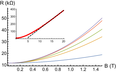
Figure 1: (Color online) Upper panel: magnetoresistance in graphene at charge neutrality. The uppermost curve shows the result (17) for a macroscopic sample. The lower curves show the result (45) for sample widths W=100,20,10,2μ𝑊10020102𝜇W=100,20,10,2\;\mum (top to bottom). The results are calculated for realistic values of parameters: T=240𝑇240{T=240} K, τ1=50superscript𝜏150{\tau^{-1}=50} K, τee=0.2τsubscript𝜏𝑒𝑒0.2𝜏{\tau_{ee}=0.2\tau}, τph=20τsubscript𝜏𝑝20𝜏{\tau_{ph}=20\tau}. The inset illustrates the linear magnetoresistance for W=0.1μ𝑊0.1𝜇W=0.1\;\mum. The dashed line is a 
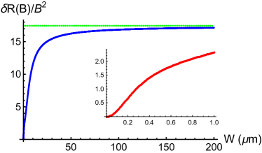
guide to the eye. Lower panel: curvature of the above magnetoresistance in weak fields (in units of kΩΩ\Omega/T2) as a function of W𝑊W. Green line shows the prefactor in Eq. (17). The inset shows the region W<1μ𝑊1𝜇{W<1\;\mu}m.

Qualitative behavior of the result (45) is determined by the interplay of sample geometry, magnetic field, and electron-phonon scattering.

In the most narrow samples (formally, in the limit ${W\rightarrow{0}}$) the square bracket in Eq. (45) vanishes and the resulting resistance is independent of the magnetic field (see Fig. 1). Physically, this happens when the electron-phonon length scale $\ell$ given by the largest eigenvalue of the operator (43b) exceeds the sample width, $W\ll\ell$.

In widest samples, ${W\gg\ell_{R}\omega_{B}^{2}\tau\tau_{ee}}$, [here $\ell_{R}$ is the recombination length given by the smallest eigenvalue of the operator (43b)] the width-dependent term in Eq. (45) can be neglected and we reproduce Eq. (17) as

$$1+\delta{\cal R}\begin{pmatrix}1&-\gamma_{2}\end{pmatrix}\widehat{\cal M}_{\cal R}^{-1}\begin{pmatrix}1\cr 1\end{pmatrix}=\left[1+\frac{{\cal R}_{H}^{2}}{{\cal R}_{0}{\cal R}_{j}}\frac{\kappa}{\Delta(0)}\right]^{-1}.$$

The result (17) is shown by the top curve in Fig. 1, where we present magnetoresistance in graphene at charge neutrality (45) for samples of different widths and for realistic sample parameters.

In narrower samples the magnetoresistance (45) weakens, see Fig. 1. In classically strong fields, ${{\cal R}_{H}\gg{\cal R}_{j}}$, one finds an intermediate regime, ${\ell_{R}\ll{W}\ll\ell_{R}\omega_{B}^{2}\tau\tau_{ee}}$, where the system exhibits linear magnetoresistance

$$R\sim B\frac{v_{g}}{c}\sqrt{\frac{{\cal R}_{j}W^{2}}{T^{3}\tau_{ph}}}.$$ (46)

The recombination length is inversely proportional to the magnetic field $\ell_{R}\sim[cT/(ev_{g}B)]\sqrt{\tau_{ph}/\tau_{ee}}$. Linear magnetoresistance is illustrated in the inset in Fig. 1.

IV Transport properties of double-layer systems

Double-layer systems are often used to study transport properties of two-dimensional systems. In comparison to single-layer devices, one can can study two additional phenomena: (i) the relatively weak effect of the second layer on the single-layer transport properties, and (ii) the strong Coulomb drag effect. The latter is due to interlayer electron-electron scattering and is important only in the academic case of disorder-free graphene in the degenerate limit, where it provides the only source of resistance. In all other cases, the effect is relatively small due to the weakness of the interlayer interaction. On the other hand, the drag effect in double-layer systems gor ; tu1 ; tu2 ; meg is solely due to the interlayer interaction and has no counterpart in non-interacting systems. Given the extensive theoretical literature devoted to Coulomb drag (see Refs. mem, ; meg, ; us1, ; thd, ; lev, and references therein), here we focus on the two following issues. Firstly, we compute the leading correction to the Fermi-liquid prediction for the drag coefficient in the degenerate regime $\mu\gg{T}$. Secondly, we discuss the drag effect at charge neutrality, where our theory provides microscopic justification to the phenomenological treatment of the effect of giant magnetodrag at charge neutrality given in Ref. meg, .

Transport properties of double-layer systems can be described within the same macroscopic approach to the Boltzmann equation as we have used above in the context of monolayer graphene. Now we introduce the system of two coupled kinetic equations similar to Eq. (18):

$\displaystyle\frac{\partial f_{1}}{\partial t}+\boldsymbol{v}_{1}\cdot\frac{\partial f_{1}}{\partial\boldsymbol{r}}+\left(e\boldsymbol{E}_{1}+\frac{e}{c}\boldsymbol{v}_{1}\times\boldsymbol{B}\right)\cdot\frac{\partial f_{1}}{\partial\boldsymbol{p}}=$ (47)
$\displaystyle\qquad\qquad\qquad\qquad=-\frac{\delta f_{1}}{\tau}+{\cal I}_{11}(f_{1})+{\cal I}_{12}(f_{1},f_{2}),$
$\displaystyle\frac{\partial f_{2}}{\partial t}+\boldsymbol{v}_{2}\cdot\frac{\partial f_{2}}{\partial\boldsymbol{r}}+\left(e\boldsymbol{E}_{2}+\frac{e}{c}\boldsymbol{v}_{2}\times\boldsymbol{B}\right)\cdot\frac{\partial f_{2}}{\partial\boldsymbol{p}}=$
$\displaystyle\qquad\qquad\qquad\qquad=-\frac{\delta f_{2}}{\tau}+{\cal I}_{22}(f_{2})+{\cal I}_{21}(f_{1},f_{2}).$

Now the distribution functions $f_{i}$ carry the layer index $i=1,2$. The single-layer collision integrals ${\cal I}_{ii}(f_{i})$ are the same as one used in the above discussion of monolayer graphene, see Eq. (63) and Appendix B.1 for details. The interlayer coupling is described by the inter-layer collision integrals ${\cal I}_{12}(f_{1},f_{2})$ and ${\cal I}_{21}(f_{1},f_{2})$, see Appendix B.2.

IV.1 Infinite system

Within linear response, deviations of the distribution functions $f_{i}$ from equilibrium can be described by Eq. (19). In an infinite system, we can still use the three-mode approximation (5) for the non-equilibrium distribution functions $h_{i}$

$$h_{i}=\frac{2\boldsymbol{v}}{e\nu_{i}Tv_{g}^{2}}\left\{\boldsymbol{\cal A}_{i}+\boldsymbol{\cal B}_{i}\frac{\epsilon}{K_{i}}+\boldsymbol{\cal C}_{i}{\rm sign}(\epsilon)\right\}.$$ (48)

The vectors in Eq. (48) can be read off Eq. (58), with the self-evident addition of the layer index.

IV.1.1 Macroscopic equations

Here we would like to describe the double-layer system similarly to the above macroscopic description of monolayer graphene. Integrating the kinetic equations (47) we obtain the following equations for the macroscopic currents (here $i$ refers to a layer, while $j$ to the other layer)

$$\boldsymbol{E}_{i}+{\cal R}_{H}^{(i)}\;\boldsymbol{\cal K}_{i}\times\boldsymbol{e}_{\boldsymbol{B}}={\cal R}_{0}^{(i)}\boldsymbol{j}_{i}-\frac{\pi}{e^{2}K_{i}}\boldsymbol{\cal I}_{ii}-\frac{\pi}{e^{2}K_{i}}\boldsymbol{\cal I}_{ij},$$ (49a)
$${\cal N}_{1}^{(i)}\boldsymbol{E}_{i}+{\cal R}_{H}^{(i)}\;\boldsymbol{j}_{i}\times\boldsymbol{e}_{\boldsymbol{B}}={\cal R}_{0}^{(i)}\frac{e}{K_{i}}\boldsymbol{Q}_{i}-\frac{\pi}{eK_{i}^{2}}\boldsymbol{\cal I}^{\prime}_{ij},$$ (49b)
$$\frac{\mu_{i}}{K_{i}}\boldsymbol{E}_{i}+{\cal R}_{H}^{(i)}\;\widetilde{\boldsymbol{\cal K}}_{i}\times\boldsymbol{e}_{\boldsymbol{B}}=e{\cal R}_{0}^{(i)}\boldsymbol{P}_{i}-\frac{\pi}{eK_{i}}\boldsymbol{\cal I}^{\prime\prime}_{ii}-\frac{\pi}{eK_{i}}\boldsymbol{\cal I}^{\prime\prime}_{ij}.$$ (49c)

Here the intralayer collision integrals $\boldsymbol{\cal I}_{ii}$ and $\boldsymbol{\cal I}^{\prime\prime}_{ii}$ are still described by Eqs. (30c) and (32c), respectively, with the obvious addition of the layer index. The interlayer collision integrals are described in detail in Appendix B.2. One can recast them in terms of relaxation rates and rewrite the equations (49) in the form (1). The resulting equations contain a rather large number of terms. Therefore, below we will discuss the most interesting limiting cases, where they can be significantly simplified.

IV.1.2 Coulomb drag in degenerate limit

In the degenerate limit Coulomb drag can be described be means of the generalized Ohm’s (or Drude) equations mem with the phenomenological term describing interlayer friction by means of the corresponding scattering time $\tau_{D}$. It is well known us1 , however, that the traditional Fermi-liquid theory of Coulomb drag is applicable only for very large densities, far beyond the current experimental range gor ; tu1 ; tu2 ; meg .

Leading corrections to the Fermi-liquid results can be described in terms of small deviations of the energy and imbalance currents from their limiting values (10). It is intuitively clear that the imbalance current approaches the limiting value exponentially. In contrast, the energy current is expected to exhibit power law corrections. These can be demonstrated by the following arguments.

The drag measurement is performed by passing a current $\boldsymbol{j}_{1}=j_{1}\boldsymbol{e}_{x}$ through one of the layers (the active layer) and measuring the induced electric field (or voltage) in the other, passive layer. Consider for simplicity identical, macroscopic layers. In the degenerate regime, we may set $e\boldsymbol{P}_{1}=\boldsymbol{j}_{1}$ (since the deviations from this equality are exponentially small in $T/\mu$), neglect small differences between various interlayer relaxation rates, disregard intralayer interaction effects, and assume interlayer thermalization that yields [see, e.g., Eq. (89)]

$$\frac{e}{\mu}\boldsymbol{Q}_{2}=\frac{e}{\mu}\boldsymbol{Q}_{1}-{\cal N}_{1}\boldsymbol{j}_{1}.$$

As a result, the macroscopic equations have the form

$$\boldsymbol{E}_{1}+{\cal R}_{H}\;\boldsymbol{\cal K}_{1}\times\boldsymbol{e}_{\boldsymbol{B}}=\left({\cal R}_{0}+{\cal R}_{D}\right)\boldsymbol{j}_{1},$$ (50a)
$${\cal N}_{1}\boldsymbol{E}_{1}+\frac{{\cal N}_{1}+1}{2}{\cal R}_{H}\;\boldsymbol{j}_{1}\times\boldsymbol{e}_{\boldsymbol{B}}={\cal R}_{0}\frac{e}{\mu}\boldsymbol{Q}_{1}+{\cal N}_{1}{\cal R}_{D}\boldsymbol{j}_{1},$$ (50b)
$$\boldsymbol{E}_{2}+{\cal R}_{H}\;\boldsymbol{\cal K}_{2}\times\boldsymbol{e}_{\boldsymbol{B}}=-{\cal R}_{D}\boldsymbol{j}_{1},$$ (50c)

where ${{\cal R}_{D}=\pi/(e^{2}\mu\tau_{D})}$ [see Eq. (76)] is the standard drag resistivity. The auxiliary vectors in the Lorentz terms read

$$\boldsymbol{\cal K}_{1}\approx\boldsymbol{j}_{1}-\left(\frac{e}{\mu}\boldsymbol{Q}_{1}-{\cal N}_{1}\boldsymbol{j}_{1}\right),\qquad\boldsymbol{\cal K}_{2}\approx-\frac{e}{\mu}\boldsymbol{Q}_{2}.$$

Neglecting small deviations of the energy current in the active layer from its limiting value $(e/\mu)\boldsymbol{Q}_{1}=\boldsymbol{j}_{1}$, we find the standard drag effect (defined according to Refs. gor, ; meg, )

$$\boldsymbol{Q}_{2}=0\quad\Rightarrow\quad R_{D}=\frac{E_{2x}}{j_{1}}=-{\cal R}_{D},$$ (51)

which is independent of magnetic field.

In contrast, taking into account a small deviation of $\boldsymbol{Q}_{1}$ from its limiting value, we find that the leading correction to $R_{D}$ depends on magnetic field

$$R_{D}=-{\cal R}_{D}+\frac{\pi^{2}T^{2}}{6\mu^{2}}\frac{{\cal R}_{H}^{2}{\cal R}_{0}}{{\cal R}_{0}^{2}+{\cal R}_{H}^{2}}.$$ (52)

Same calculation also yields the Hall drag resistivity:

$$R_{DH}=\frac{E_{2y}}{j_{1}}=-\frac{\pi^{2}T^{2}}{6\mu^{2}}\frac{{\cal R}_{H}^{3}}{{\cal R}_{0}^{2}+{\cal R}_{H}^{2}}.$$ (53)

In contrast to the traditional theories of Coulomb drag, the above results contain contributions that do not directly depend on any interlayer electron-electron scattering rate. Instead, this is the effect of interlayer thermalization.

At the same time, the presence of the second layer leads to the appearance of magnetoresistance in the first layer (which vanishes in the limit $\mu\rightarrow\infty$)

$$R(\mu\gg T)={\cal R}_{0}+{\cal R}_{D}+\frac{\pi^{2}T^{2}}{6\mu^{2}}\frac{{\cal R}_{H}^{2}{\cal R}_{0}}{{\cal R}_{0}^{2}+{\cal R}_{H}^{2}},$$ (54)

as well as a small correction to the Hall coefficient

$$R_{H}(\mu\gg T)={\cal R}_{H}-\frac{\pi^{2}T^{2}}{6\mu^{2}}\frac{{\cal R}_{H}^{3}}{{\cal R}_{0}^{2}+{\cal R}_{H}^{2}}.$$ (55)

The above corrections exhibit power-law dependence on the small ratio $T/\mu$. This is in contrast to the exponential approach to the Fermi-liquid limit that was found within the two-mode approximation in Ref. meg, , as illustrated in Fig. 2. Indeed, the phenomenological model of Ref. meg, included the electric and imbalance currents. The latter approaches its limiting value $e\boldsymbol{P}_{1}=\boldsymbol{j}_{1}$ only exponentially. Hence the exponentially small magnetodrag in doped graphene found in Ref. meg, (in notable disagreement with experimental data) is an artifact of neglecting the energy current in the simplified phenomenological model. At the same time, at charge neutrality the imbalance current is proportional to the energy current while both are orthogonal to $\boldsymbol{j}$. Hence the phenomenological model of Ref. meg, captures qualitative physics at the Dirac point, see below.

Refer to caption

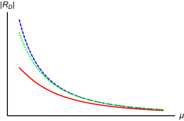
Figure 2: (Color online) Schematic illustration of corrections to the Fermi-liquid predictions for the drag coefficient. The blue dashed curve represents the Fermi-liquid result ${\cal R}_{D}\sim T^{2}/\mu^{2}$. The green dotted curve represents the exponential approach to ${\cal R}_{D}$ within the two-mode approximation that retains the electric and imbalance currents. The red solid line shows the result (52) of the three-mode approximation approaching the Fermi-liquid regime as a power law in $T/\mu$.

IV.1.3 Macroscopic theory at the neutrality point

At the charge neutrality (or double Dirac) point we may consider the two layers to be identical. With the help of the thermalization conditions (90) and Eqs. (13), we find the following macroscopic description of an infinite double-layer system [cf. Eqs. (14)]. The first layer is described by the equations [with the auxiliary vectors given by Eqs. (13)]

$$\boldsymbol{E}_{1}+{\cal R}_{H}\;\boldsymbol{\cal K}_{1}\times\boldsymbol{e}_{\boldsymbol{B}}=\left[{\cal R}_{j}+\frac{\pi}{2e^{2}T\tau_{vv,12}\ln 2}\right]\boldsymbol{j}_{1},$$ (56a)
$$\frac{1}{2}{\cal R}_{H}\;\boldsymbol{j}_{1}\times\boldsymbol{e}_{\boldsymbol{B}}={\cal R}_{0}^{(1)}\frac{e}{2T\ln 2}\boldsymbol{Q}_{1},$$ (56b)
$$\frac{1}{2}{\cal R}_{H}\;\boldsymbol{j}_{1}\times\boldsymbol{e}_{\boldsymbol{B}}=e{\cal R}_{0}^{(1)}\boldsymbol{P}_{1}+\frac{\pi\left(\tau_{ss}^{-1}+\tau_{ss,12}^{-1}\right)}{2e^{2}T\ln 2}\boldsymbol{\cal C}_{1}.$$ (56c)
The energy and imbalance currents in the second layer are determined by the thermalization conditions (90). The equation for the electric current is similar to Eq. (56a). However, if we consider the typical setup for drag measurements, where no electric current is allowed to flow in the second layer, then the equation simplifies to
$$\boldsymbol{E}_{2}+{\cal R}_{H}\;\boldsymbol{\cal K}_{1}\times\boldsymbol{e}_{\boldsymbol{B}}=0.$$ (56d)

The solution of the equations (56) is identical to that described in Section I. The presence of the second layer does not significantly change transport in the first layer, in particular, Eqs. (56) still predict positive magnetoresistance. The Hall classical effect does not appear at charge neutrality as it should be.

For the second layer, this theory predicts positive Coulomb drag [defined in Eq. (51)] in agreement with qualitative arguments of Ref. meg, . In order to explain the experimentally observed negative drag gor ; meg the theory needs to be refined as follows: (i) the finite width $W$ of the system should be taken into account; the relative parameter is $W/\ell_{R}$, where $\ell_{R}$ is the phonon-induced relaxation length, see Section III; (ii) the above interlayer thermalization procedure should be improved to take into account the finite interlayer electron-electron relaxation rate. This is outlined in Section IV.2.

IV.2 Mesoscopic system at charge neutrality

In a mesoscopic system, we need to take into account spatial inhomogeneity of the macroscopic currents and densities. In this case, the non-equilibrium distribution function acquires the additional contribution (28)

$$\delta h_{i}=\frac{1}{e\nu_{i}T}\left[\mathfrak{a}_{i}+\mathfrak{b}_{i}\frac{\epsilon}{K_{i}}+\mathfrak{c}_{i}\;{\rm sign}(\epsilon)\right].$$ (57)

Similarly to the situation in monolayer graphene, macroscopic equations in double-layer systems acquire gradient terms. The resulting equations contain two copies of Eqs. (1) where one has to add interlayer scattering rates from the right-hand side of Eqs. (49), two copies of continuity equations similar to Eqs. (9) where one has to include additional contributions due to interlayer electron-electron interaction (see Appendix D), and the Maxwell equations (8). A general solution to this system of equations is rather convoluted. Hence here we limit ourselves to a qualitative discussion.

Of particular interest is the drag effect at charge neutrality, where the experiment gor ; meg shows an unusually strong dependence of $R_{D}$ on the external magnetic field, i.e. giant magnetodrag. The problem of Coulomb drag in graphene at charge neutrality was previously addressed in Refs. meg, ; lev, based on a two-fluid approach. As shown in Section III above, the energy and imbalance currents in the active layer at the neutrality point are parallel to each other and orthogonal to the driving current ${\boldsymbol{Q}_{1}\|\boldsymbol{P}_{1}\perp\boldsymbol{j}_{1}}$. Excluding one of these currents from the macroscopic equations one effectively derives a two-fluid model. Thus our theory provides a microscopic foundation for the earlier phenomenological models. The key point is that the currents $\boldsymbol{Q}$ and $\boldsymbol{P}$ can be transferred between the layers by means of the interlayer interaction in contrast to the electric current, whose transfer is forbidden by the exact electron-hole symmetry at the Dirac point.

In the limit of infinitely fast interlayer thermalization (discussed above in Section IV.1.2) the energy and imbalance currents in the two layers have the same direction leading to positive drag. Taking into account finiteness of the corresponding relaxation rates (Appendix D) refines the theory in analogy with including viscous terms into standard hydrodynamic theory dau ; ulf . The resulting theory contains four differential equations for the energy and imbalance currents [cf. Eq. (42a) in the single-layer case]. If the sample is wide enough (i.e. if the width of the sample $W$ is larger than the phonon-induced recombination length), the energy and imbalance currents in the two layers flow in the same direction and the system exhibits positive drag as discussed above. On the contrary, in narrow samples it is the inhomogeneous energy and imbalance densities in the two layers that coincide, pushing the currents in the opposite directions and yielding negative drag meg ; lev . Similarly to the discussion in Section III, the magnetic field dependence of the result is quadratic in weak fields and linear in classically strong fields.

V Summary

We have developed a macroscopic (hydrodynamic-like) description of electronic transport in graphene. Our approach is based on the “three-mode” Ansatz for the non-equilibrium distribution function in graphene. This Ansatz is justified in the interaction-dominated regime by the collinear scattering singularity in the collision integral. Under such assumptions, transport properties of graphene can be described in terms of the three macroscopic currents, $\boldsymbol{j}$, $\boldsymbol{P}$, and $\boldsymbol{Q}$. In small, mesoscopic samples physical properties become inhomogeneous and we need to introduce the inhomogeneous corrections to the corresponding charge, energy, and imbalance densities. In that case, the complete set of macroscopic equations includes three equations (1) for the currents, which can be viewed as the generalization of the Ohm’s law, three continuity equations, and the Maxwell equations, describing the self-consistent electromagnetic field.

Solving the macroscopic equations, one can find temperature, density, and geometry (i.e. the system size) dependence of transport coefficients. For general doping this is a formidable computational task. However, far away from charge neutrality (in the degenerate or “Fermi-liquid” regime) all the three currents become equivalent and the theory reduces to the single-mode equation (11) with the Drude transport coefficients (12) as it should, given that no quantum interference processes were taken into account.

Exactly at the Dirac point, the theory simplifies as well and allows for analytic solutions. We have shown that graphene at charge neutrality exhibits strong positive magnetoresistance (45). Specifically, the resistance behaves quadratically in not too strong fields, Eq. (17), and crosses over to the linear dependence (46) once the field increases beyond a certain value determined by the sample width and quasiparticle recombination rate due to electron-phonon interaction, see Fig. 1.

Strong positive magnetoresistance in graphene was observed in Refs. fu1, ; fu2, ; job, ; mg3, at charge neutrality. Our results qualitatively agree with the experimental data. Moreover, our theory can be generalized to account for macroscopic inhomogeneities that were discussed as a possible source of magnetoresistance in Refs. fu1, ; fu2, . Further experimental studies of magnetoresistance in high-mobility graphene samples (including the dependence on the sample width) would be of great interest.

In double-layer systems, our theory provides the microscopic justification of the phenomenological treatment of the giant magnetodrag problem suggested in Ref. meg, . The three-mode Ansatz allows for more precise quantitative description of the effect. In particular, we have calculated the leading correction to the Fermi-liquid prediction for the drag coefficient in doped graphene. Physically, the resulting magnetodrag (52), as well as Hall drag (53) is due to interlayer thermalization. Treating all three modes on equal footing allows us to remove the artifacts of two-mode approximations, see Fig. 2.

In this paper we have limited ourselves to linear response theory. A generalization of our approach to nonlinear hydrodynamics in graphene will be reported in a subsequent publication ulf .

Acknowledgements.
We acknowledge helpful conversations with H. Weber, U. Briskot, A. Levchenko, L. Ponomarenko, P. Alekseev, V. Kachorovsky, Yu. Vasiliev, and A. Dmitriev. This work was supported by the Dutch Science Foundation NWO/FOM 13PR3118, the EU Network Grant InterNoM, DFG-SPP 1459, DFG-SPP 1666, GIF, and the Humboldt Foundation.

Appendix A Non-equilibrium distribution function in the three-mode approximation

In this Appendix we give the complete expression for the non-equilibrium distribution function $h$ in monolayer graphene in terms of the three macroscopic currents (21) and densities (25)

$\displaystyle h=\frac{2\boldsymbol{v}}{e\nu_{0}Tv_{g}^{2}}\left\{\boldsymbol{\cal A}+\boldsymbol{\cal B}\frac{\epsilon}{K}+\boldsymbol{\cal C}{\rm sign}(\epsilon)\right\},$ (58a)
$$\boldsymbol{\cal A}=\boldsymbol{j}+\frac{\frac{e}{K}\boldsymbol{Q}-{\cal N}_{1}\boldsymbol{j}}{\Delta}\left[{\cal N}_{1}-\frac{\mu T^{2}}{K^{3}}\left(\frac{\pi^{2}}{3}+\frac{\mu^{2}}{T^{2}}\right)\right]+\frac{e\boldsymbol{P}-\frac{\mu}{K}\boldsymbol{j}}{\Delta}\left[{\cal N}_{2}\frac{\mu}{K}-{\cal N}_{1}\frac{T^{2}}{K^{2}}\left(\frac{\pi^{2}}{3}+\frac{\mu^{2}}{T^{2}}\right)\right],$$ (58b)
$$\boldsymbol{\cal B}=\frac{\frac{e}{K}\boldsymbol{Q}-{\cal N}_{1}\boldsymbol{j}}{\Delta}\left(\frac{\mu^{2}}{K^{2}}-1\right)+\frac{e\boldsymbol{P}-\frac{\mu}{K}\boldsymbol{j}}{\Delta}\left[\frac{T^{2}}{K^{2}}\left(\frac{\pi^{2}}{3}+\frac{\mu^{2}}{T^{2}}\right)-{\cal N}_{1}\frac{\mu}{K}\right]$$ (58c)
$$\boldsymbol{\cal C}=\frac{\frac{e}{K}\boldsymbol{Q}-{\cal N}_{1}\boldsymbol{j}}{\Delta}\left[\frac{T^{2}}{K^{2}}\left(\frac{\pi^{2}}{3}+\frac{\mu^{2}}{T^{2}}\right)-{\cal N}_{1}\frac{\mu}{K}\right]+\frac{e\boldsymbol{P}-\frac{\mu}{K}\boldsymbol{j}}{\Delta}\left[{\cal N}_{1}^{2}-{\cal N}_{2}\right]$$ (58d)
$\displaystyle\delta h=\frac{1}{e\nu_{0}T}\left[\mathfrak{a}+\mathfrak{b}\frac{\epsilon}{K}+\mathfrak{c}\;{\rm sign}(\epsilon)\right],$ (59a)
$$\mathfrak{a}=\delta n+\frac{\frac{e}{K}\delta u-{\cal N}_{1}\delta n}{\Delta}\left[{\cal N}_{1}-\frac{\mu T^{2}}{K^{3}}\left(\frac{\pi^{2}}{3}+\frac{\mu^{2}}{T^{2}}\right)\right]+\frac{e\delta\rho-\frac{\mu}{K}\delta n}{\Delta}\left[{\cal N}_{2}\frac{\mu}{K}-{\cal N}_{1}\frac{T^{2}}{K^{2}}\left(\frac{\pi^{2}}{3}+\frac{\mu^{2}}{T^{2}}\right)\right],$$ (59b)
$$\mathfrak{b}=\frac{\frac{e}{K}\delta u-{\cal N}_{1}\delta n}{\Delta}\left(\frac{\mu^{2}}{K^{2}}-1\right)+\frac{e\delta\rho-\frac{\mu}{K}\delta n}{\Delta}\left[\frac{T^{2}}{K^{2}}\left(\frac{\pi^{2}}{3}+\frac{\mu^{2}}{T^{2}}\right)-{\cal N}_{1}\frac{\mu}{K}\right]$$ (59c)
$$\mathfrak{c}=\frac{\frac{e}{K}\delta u-{\cal N}_{1}\delta n}{\Delta}\left[\frac{T^{2}}{K^{2}}\left(\frac{\pi^{2}}{3}+\frac{\mu^{2}}{T^{2}}\right)-{\cal N}_{1}\frac{\mu}{K}\right]+\frac{e\delta\rho-\frac{\mu}{K}\delta n}{\Delta}\left[{\cal N}_{1}^{2}-{\cal N}_{2}\right]$$ (59d)

where ${\cal N}_{1}$ is a dimensionless quantity proportional to the carrier density in graphene

$\displaystyle n_{0}=\int\limits_{-\infty}^{\infty}d\epsilon\,\nu(\epsilon)\left[f^{(0)}(\epsilon;\mu)-f^{(0)}(\epsilon;0)\right],\qquad\sum\epsilon\left(-\frac{\partial f^{(0)}}{\partial\epsilon}\right)=2n_{0},\qquad 2n_{0}={\cal N}\nu_{0}\mu={\cal N}_{1}\nu_{0}K.$ (60a)
This dimensionless function depends only on the ratio $x=\mu/T$ and has the following asymptotic behavior:
$\displaystyle{\cal N}(x)\approx\left\{\begin{matrix}2-\frac{x^{2}}{6\ln 2}+\dots,&x\ll 1,\cr\cr 1+\frac{\pi^{2}}{3x^{2}}+\dots,&x\gg 1,\end{matrix}\right.,\qquad\qquad{\cal N}_{1}(x)\approx\left\{\begin{matrix}\frac{x}{\ln 2}\left[1-\frac{5x^{2}}{24\ln 2}+\dots\right],&x\ll 1,\cr\cr 1+\frac{\pi^{2}}{3x^{2}}+\dots,&x\gg 1.\end{matrix}\right.$ (60b)

Similarly, the dimensionless quantity ${\cal N}_{2}$ represents a similar sum

$\displaystyle{\cal N}_{2}(x)=\frac{1}{\nu_{0}K^{2}}\sum\epsilon^{2}\left(-\frac{\partial f^{(0)}}{\partial\epsilon}\right)\approx\left\{\begin{matrix}\frac{9\zeta(3)}{8\ln^{3}2}+\frac{3}{4\ln^{2}2}\left(1-\frac{9\zeta(3)}{16\ln^{2}2}\right)x^{2},&x\ll 1,\cr\cr 1+\frac{\pi^{2}}{x^{2}},&x\gg 1.\end{matrix}\right.,$ (61)

and the dimensionless quantity $\Delta$ is

$\displaystyle\Delta=\left[\frac{T^{2}}{K^{2}}\left(\frac{\pi^{2}}{3}+\frac{\mu^{2}}{T^{2}}\right)-{\cal N}_{1}\frac{\mu}{K}\right]^{2}+\left({\cal N}_{2}-{\cal N}_{1}^{2}\right)\left(\frac{\mu^{2}}{K^{2}}-1\right)\approx\left\{\begin{matrix}-1.13025+0.9348x^{2},&x\ll 1,\cr\cr-\frac{4\pi^{2}}{3x^{3}}e^{-x},&x\gg 1.\end{matrix}\right..$ (62)

Appendix B Relaxation rates due to electron-electron interaction

B.1 Monolayer graphene

Within linear response the collision integral in Eq. (18) can be linearized with the help of Eq. (19) as follows

$\displaystyle{\cal I}=\sum_{1,1^{\prime},2^{\prime}}W_{12,1^{\prime}2^{\prime}}f^{(0)}_{1}f^{(0)}_{2}\left[1-f^{(0)}_{1^{\prime}}\right]\left[1-f^{(0)}_{2^{\prime}}\right]\left[h_{1^{\prime}}+h_{2^{\prime}}-h_{1}-h_{2}\right].$ (63)

B.1.1 Collision term in the equation for the electric current

Following the usual steps involving introduction of transferred energy $\omega$ and momentum $\boldsymbol{q}$, we find for the integrated collision integral Eq. (30c) appearing in the equation (30) for the electric current:

$\displaystyle\boldsymbol{\cal I}=-\frac{e}{32}\int\frac{d^{2}qd\omega}{(2\pi)^{3}}\frac{|U(\boldsymbol{q},\omega)|^{2}}{\sinh^{2}(\omega/2T)}$ (64)
$\displaystyle\qquad\qquad\qquad\times\sum_{1,1^{\prime}}(2\pi)^{3}|\lambda_{\boldsymbol{v}\boldsymbol{v}^{\prime}}|^{2}\delta(\epsilon_{1}-\epsilon_{1}^{\prime}+\omega)\delta(\boldsymbol{p}_{1}-\boldsymbol{p}_{1}^{\prime}+\boldsymbol{q})\left[\tanh\frac{\epsilon_{1}-\mu}{2T}-\tanh\frac{\epsilon_{1}+\omega-\mu}{2T}\right]$
$\displaystyle\qquad\qquad\qquad\times\sum_{2,2^{\prime}}(\boldsymbol{v}_{2}-\boldsymbol{v}_{2}^{\prime})(2\pi)^{3}|\lambda_{\boldsymbol{v}\boldsymbol{v}^{\prime}}|^{2}\delta(\epsilon_{2}-\epsilon_{2}^{\prime}-\omega)\delta(\boldsymbol{p}_{2}-\boldsymbol{p}_{2}^{\prime}-\boldsymbol{q})\left[\tanh\frac{\epsilon_{2}-\mu}{2T}-\tanh\frac{\epsilon_{2}-\omega-\mu}{2T}\right]$
$\displaystyle\qquad\qquad\qquad\times\left[h_{1^{\prime}}+h_{2^{\prime}}-h_{1}-h_{2}\right].$

Here $|\lambda_{\boldsymbol{v}\boldsymbol{v}^{\prime}}|^{2}$ are the “Dirac factors”.

Taking into account the explicit form of the distribution function (5), summations over states $1,1^{\prime}$ and $2,2^{\prime}$ factorize. Consequently, one can evaluate them separately. The resulting expressions can be denoted as follows:

$\displaystyle(2\pi)^{3}\sum_{1,1^{\prime}}|\lambda_{\boldsymbol{v}\boldsymbol{v}^{\prime}}|^{2}\delta(\epsilon_{1}-\epsilon_{1}^{\prime}+\omega)\delta(\boldsymbol{p}_{1}-\boldsymbol{p}_{1}^{\prime}+\boldsymbol{q})\left[\tanh\frac{\epsilon_{1}-\mu}{2T}-\tanh\frac{\epsilon_{1}+\omega-\mu}{2T}\right]=Y_{00}(\boldsymbol{q},\omega),$ (65a)
$\displaystyle(2\pi)^{3}\sum_{1,1^{\prime}}\left(\boldsymbol{v}_{1}^{\prime}-\boldsymbol{v}_{1}\right)|\lambda_{\boldsymbol{v}\boldsymbol{v}^{\prime}}|^{2}\delta(\epsilon_{1}-\epsilon_{1}^{\prime}+\omega)\delta(\boldsymbol{p}_{1}-\boldsymbol{p}_{1}^{\prime}+\boldsymbol{q})\left[\tanh\frac{\epsilon_{1}-\mu}{2T}-\tanh\frac{\epsilon_{1}+\omega-\mu}{2T}\right]=\frac{\boldsymbol{q}}{q}v_{g}Y_{0A}(\boldsymbol{q},\omega),$ (65b)
$$(2\pi)^{3}\sum_{1,1^{\prime}}\left(\boldsymbol{v}_{1}^{\prime}{\rm sgn}\;\epsilon_{1}^{\prime}-\boldsymbol{v}_{1}{\rm sgn}\;\epsilon_{1}\right)|\lambda_{\boldsymbol{v}\boldsymbol{v}^{\prime}}|^{2}\delta(\epsilon_{1}-\epsilon_{1}^{\prime}+\omega)\delta(\boldsymbol{p}_{1}-\boldsymbol{p}_{1}^{\prime}+\boldsymbol{q})\left[\tanh\frac{\epsilon_{1}-\mu}{2T}-\tanh\frac{\epsilon_{1}+\omega-\mu}{2T}\right]=\frac{\boldsymbol{q}}{q}v_{g}Y_{0C}(\boldsymbol{q},\omega),$$ (65c)
$\displaystyle(2\pi)^{3}\sum_{1,1^{\prime}}\left(v_{1}^{\prime\alpha}-v_{1}^{\alpha}\right)\left(v_{1}^{\prime\beta}-v_{1}^{\beta}\right)|\lambda_{\boldsymbol{v}\boldsymbol{v}^{\prime}}|^{2}\delta(\epsilon_{1}-\epsilon_{1}^{\prime}+\omega)\delta(\boldsymbol{p}_{1}-\boldsymbol{p}_{1}^{\prime}+\boldsymbol{q})$
$\displaystyle\qquad\qquad\qquad\qquad\qquad\qquad\qquad\times\left[\tanh\frac{\epsilon_{1}-\mu}{2T}-\tanh\frac{\epsilon_{1}+\omega-\mu}{2T}\right]=\frac{q^{\alpha}q^{\beta}}{q^{2}}v_{g}^{2}Y_{AA}(\boldsymbol{q},\omega),$ (65d)
$\displaystyle(2\pi)^{3}\sum_{1,1^{\prime}}\left(v_{1}^{\prime\alpha}-v_{1}^{\alpha}\right)\left(v_{1}^{\prime\beta}{\rm sgn}\;\epsilon_{1}^{\prime}-v_{1}^{\beta}{\rm sgn}\;\epsilon_{1}\right)|\lambda_{\boldsymbol{v}\boldsymbol{v}^{\prime}}|^{2}\delta(\epsilon_{1}-\epsilon_{1}^{\prime}+\omega)\delta(\boldsymbol{p}_{1}-\boldsymbol{p}_{1}^{\prime}+\boldsymbol{q})$
$\displaystyle\qquad\qquad\qquad\qquad\qquad\qquad\qquad\times\left[\tanh\frac{\epsilon_{1}-\mu}{2T}-\tanh\frac{\epsilon_{1}+\omega-\mu}{2T}\right]=\frac{q^{\alpha}q^{\beta}}{q^{2}}v_{g}^{2}Y_{AC}(\boldsymbol{q},\omega),$ (65e)

All of thus defined functions $Y_{ij}(\boldsymbol{q},\omega)$ obey the trivial symmetry property

$\displaystyle Y_{ij}(\boldsymbol{q},\omega)=-Y_{ij}(-\boldsymbol{q},-\omega).$ (66)

Since the collision integral ${\cal I}$ has the dimension of inverse time, it is convenient to introduce the transport scattering times due to Coulomb interaction. Given the multitude of terms in the kinetic equation, we choose to define several interaction-related time scales. In the current equation, two such time scales appear (if the arguments of $Y_{i}(\boldsymbol{q},\omega)$ have their standard form we omit them for brevity):

$\displaystyle\frac{1}{\tau_{vv}}=\frac{1}{\nu_{0}}\sqint\left(Y_{00}Y_{AA}-Y_{0A}^{2}\right),\qquad{\rm where}\qquad\sqint\dots=\frac{e}{32T}\int\frac{d^{2}qd\omega}{(2\pi)^{3}}\frac{|U(\boldsymbol{q},\omega)|^{2}}{\sinh^{2}(\omega/2T)}\dots,$ (67)
$\displaystyle\frac{1}{\tau_{vs}}=\frac{1}{\nu_{0}}\sqint\left(Y_{00}Y_{AC}-Y_{0A}Y_{0C}\right).$ (68)

Both time scales $\tau_{vv}^{-1}$ and $\tau_{vs}^{-1}$ vanish in the Fermi-liquid limit (physically, due to the restored Galilean invariance). On the other hand, at charge neutrality $\tau_{vs}^{-1}=0$, since

$$Y_{0A}(\mu=0)=Y_{AC}(\mu=0)=0,$$ (69)

while $\tau_{vv}^{-1}$ remains finite.

Using the above relaxation rates, we can write the integrated collision integral in equation (30) in the form (30c).

B.1.2 Collision term in the equation for the imbalance current

Treating the collision integral in Eq. (32) in the same way as Eq. (64) above, we find:

$\displaystyle\boldsymbol{\cal I}^{\prime\prime}=-\frac{1}{32}\int\frac{d^{2}qd\omega}{(2\pi)^{3}}\frac{|U(\boldsymbol{q},\omega)|^{2}}{\sinh^{2}(\omega/2T)}$ (70)
$\displaystyle\qquad\qquad\times\sum_{1,1^{\prime}}(2\pi)^{3}|\lambda_{\boldsymbol{v}\boldsymbol{v}^{\prime}}|^{2}\delta(\epsilon_{1}-\epsilon_{1}^{\prime}+\omega)\delta(\boldsymbol{p}_{1}-\boldsymbol{p}_{1}^{\prime}+\boldsymbol{q})\left[\tanh\frac{\epsilon_{1}-\mu}{2T}-\tanh\frac{\epsilon_{1}+\omega-\mu}{2T}\right]$
$\displaystyle\qquad\qquad\times\sum_{2,2^{\prime}}(\boldsymbol{v}_{2}{\rm sgn}\;\epsilon_{2}-\boldsymbol{v}_{2}^{\prime}{\rm sgn}\;\epsilon_{2}^{\prime})(2\pi)^{3}|\lambda_{\boldsymbol{v}\boldsymbol{v}^{\prime}}|^{2}\delta(\epsilon_{2}-\epsilon_{2}^{\prime}-\omega)\delta(\boldsymbol{p}_{2}-\boldsymbol{p}_{2}^{\prime}-\boldsymbol{q})\left[\tanh\frac{\epsilon_{2}-\mu}{2T}-\tanh\frac{\epsilon_{2}-\omega-\mu}{2T}\right]$
$\displaystyle\qquad\qquad\times\left[h_{1^{\prime}}+h_{2^{\prime}}-h_{1}-h_{2}\right].$

Following the same line of argument as in the previous Appendix, we introduce another time scale

$\displaystyle\frac{1}{\tau_{ss}}=\frac{1}{\nu_{0}}\sqint\left(Y_{00}Y_{CC}-Y_{0C}^{2}\right),$ (71)

where we had to introduce another quantity $Y_{CC}$ similarly to Eqs. (65):

$\displaystyle(2\pi)^{3}\sum_{1,1^{\prime}}\left(v_{1}^{\prime\alpha}{\rm sgn}\;\epsilon_{1}^{\prime}-v_{1}^{\alpha}{\rm sgn}\;\epsilon_{1}\right)\left(v_{1}^{\prime\beta}{\rm sgn}\;\epsilon_{1}^{\prime}-v_{1}^{\beta}{\rm sgn}\;\epsilon_{1}\right)|\lambda_{\boldsymbol{v}\boldsymbol{v}^{\prime}}|^{2}$
$\displaystyle\qquad\qquad\qquad\times\delta(\epsilon_{1}-\epsilon_{1}^{\prime}+\omega)\delta(\boldsymbol{p}_{1}-\boldsymbol{p}_{1}^{\prime}+\boldsymbol{q})\left[\tanh\frac{\epsilon_{1}-\mu}{2T}-\tanh\frac{\epsilon_{1}+\omega-\mu}{2T}\right]=\frac{q^{\alpha}q^{\beta}}{q^{2}}v_{g}^{2}Y_{CC}(\boldsymbol{q},\omega).$ (72)

As a result, the integrated collision term (70) takes the form (32c).

B.2 Double-layer system

B.2.1 Collision term in the equation for the electric current

The integrated inter-layer collision integral has a form, similar to Eq. (64),

$\displaystyle\boldsymbol{\cal I}_{12}=-\frac{e}{32}\int\frac{d^{2}qd\omega}{(2\pi)^{3}}\frac{|U_{12}(\boldsymbol{q},\omega)|^{2}}{\sinh^{2}(\omega/2T)}$ (73)
$\displaystyle\qquad\qquad\qquad\times\sum_{1,1^{\prime}}(2\pi)^{3}|\lambda_{\boldsymbol{v}\boldsymbol{v}^{\prime}}|^{2}\delta(\epsilon_{1}-\epsilon_{1}^{\prime}+\omega)\delta(\boldsymbol{p}_{1}-\boldsymbol{p}_{1}^{\prime}+\boldsymbol{q})\left[\tanh\frac{\epsilon_{1}-\mu_{2}}{2T}-\tanh\frac{\epsilon_{1}+\omega-\mu_{2}}{2T}\right]$
$\displaystyle\qquad\qquad\qquad\times\sum_{2,2^{\prime}}(\boldsymbol{v}_{2}-\boldsymbol{v}_{2}^{\prime})(2\pi)^{3}|\lambda_{\boldsymbol{v}\boldsymbol{v}^{\prime}}|^{2}\delta(\epsilon_{2}-\epsilon_{2}^{\prime}-\omega)\delta(\boldsymbol{p}_{2}-\boldsymbol{p}_{2}^{\prime}-\boldsymbol{q})\left[\tanh\frac{\epsilon_{2}-\mu_{1}}{2T}-\tanh\frac{\epsilon_{2}-\omega-\mu_{1}}{2T}\right]$
$\displaystyle\qquad\qquad\qquad\times\left[h_{2,1^{\prime}}+h_{1,2^{\prime}}-h_{2,1}-h_{1,2}\right],$

except than now the chemical potentials and the non-equilibrium distribution functions carry the layer index (i.e. $h_{2,1}$ stands for the distribution function in layer $2$ describing the state $1$) and the potential $U_{12}(\boldsymbol{q},\omega)$ describes interlayer interaction.

Consequently, the auxiliary functions (65) as well as the densities of states, will now also acquire the layer index. This leads to a larger number of decay rates in comparison to $\tau_{ee}^{-1}$ and $\tau_{s}^{-1}$. Since most of them vanish at the Dirac point, we express the collision integral (73) as follows:

$\displaystyle\boldsymbol{\cal I}_{12}=-\boldsymbol{\cal A}_{1}\frac{e}{\nu_{01}}\oint Y_{AA}^{(1)}Y_{00}^{(2)}+\boldsymbol{\cal A}_{2}\frac{e}{\nu_{02}}\oint Y_{0A}^{(1)}Y_{0A}^{(2)}-\boldsymbol{\cal B}_{1}\frac{ev_{g}}{\nu_{01}K_{1}}\oint qY_{0A}^{(1)}Y_{00}^{(2)}$ (74)
$\displaystyle\qquad\qquad\qquad+\boldsymbol{\cal B}_{2}\frac{ev_{g}}{\nu_{02}K_{2}}\oint qY_{0A}^{(1)}Y_{00}^{(2)}-\boldsymbol{\cal C}_{1}\frac{e}{\nu_{01}}\oint Y_{AC}^{(1)}Y_{00}^{(2)}+\boldsymbol{\cal C}_{2}\frac{e}{\nu_{02}}\oint Y_{0A}^{(1)}Y_{0C}^{(2)},$

where

$$\oint\dots=\frac{1}{32T}\int\frac{d^{2}qd\omega}{(2\pi)^{3}}\frac{|U_{12}(\boldsymbol{q},\omega)|^{2}}{\sinh^{2}(\omega/2T)}\dots.$$ (75)

The first two terms are familiar from the traditional theory of Coulomb drag us1 . In particular, the usual “drag rate” $\tau_{D}^{-1}$ is given by the second term

$$\frac{1}{\tau_{D}}=\frac{e}{\nu_{02}}\oint Y_{0A}^{(1)}Y_{0A}^{(2)}.$$ (76)

In the degenerate regime, the relaxation rates in the first two terms become identical. The traditional theory is then recovered by taking into account interlayer thermalization, see below.

At the neutrality point this expression simplifies significantly. Indeed, taking into account Eq. (69) we find

$$\boldsymbol{\cal I}_{12}(\mu_{1}=\mu_{2}=0)=-\boldsymbol{\cal A}_{1}\frac{e}{\nu_{0}}\oint Y_{AA}Y_{00}=-\frac{\boldsymbol{\cal A}_{1}}{\tau_{vv,12}},$$ (77)

where the layer indices can be omitted since at the neutrality point the layers are identical to each other. On the other hand, the new relaxation rate $1/\tau_{ee,12}$ differs from Eq. (67) insofar it reflects the interlayer interaction potential $U_{12}(\boldsymbol{q},\omega)$.

B.2.2 Collision term in the equation for the energy current

The equation for the energy current is obtained by multiplying the kinetic equation by $\epsilon\boldsymbol{v}$ and integrating over all states. Then, similarly to Eq. (73) we find

$\displaystyle\boldsymbol{\cal I}^{\prime}_{12}=-\frac{1}{32}\int\frac{d^{2}qd\omega}{(2\pi)^{3}}\frac{|U_{12}(\boldsymbol{q},\omega)|^{2}}{\sinh^{2}(\omega/2T)}$ (78)
$\displaystyle\qquad\qquad\qquad\times\sum_{1,1^{\prime}}(2\pi)^{3}|\lambda_{\boldsymbol{v}\boldsymbol{v}^{\prime}}|^{2}\delta(\epsilon_{1}-\epsilon_{1}^{\prime}+\omega)\delta(\boldsymbol{p}_{1}-\boldsymbol{p}_{1}^{\prime}+\boldsymbol{q})\left[\tanh\frac{\epsilon_{1}-\mu_{2}}{2T}-\tanh\frac{\epsilon_{1}+\omega-\mu_{2}}{2T}\right]$
$\displaystyle\qquad\qquad\qquad\times\sum_{2,2^{\prime}}(\epsilon_{2}\boldsymbol{v}_{2}-\epsilon_{2}^{\prime}\boldsymbol{v}_{2}^{\prime})(2\pi)^{3}|\lambda_{\boldsymbol{v}\boldsymbol{v}^{\prime}}|^{2}\delta(\epsilon_{2}-\epsilon_{2}^{\prime}-\omega)\delta(\boldsymbol{p}_{2}-\boldsymbol{p}_{2}^{\prime}-\boldsymbol{q})\left[\tanh\frac{\epsilon_{2}-\mu_{1}}{2T}-\tanh\frac{\epsilon_{2}-\omega-\mu_{1}}{2T}\right]$
$\displaystyle\qquad\qquad\qquad\times\left[h_{2,1^{\prime}}+h_{1,2^{\prime}}-h_{2,1}-h_{1,2}\right],$

where (due to momentum conservation)

$$\epsilon_{2}\boldsymbol{v}_{2}-\epsilon_{2}^{\prime}\boldsymbol{v}_{2}^{\prime}=v_{g}^{2}\boldsymbol{q}.$$ (79)

In contrast to monolayer graphene [see Eq. (31b)], the integrated collision integral in the double-layer system does not vanish. Similarly to Eq. (74) we find

$\displaystyle\boldsymbol{\cal I}^{\prime}_{12}=-\boldsymbol{\cal A}_{1}\frac{v_{g}}{\nu_{01}}\oint qY_{0A}^{(1)}Y_{00}^{(2)}+\boldsymbol{\cal A}_{2}\frac{v_{g}}{\nu_{02}}\oint qY_{00}^{(1)}Y_{0A}^{(2)}-\boldsymbol{\cal B}_{1}\frac{v_{g}^{2}}{\nu_{01}K_{1}}\oint q^{2}Y_{00}^{(1)}Y_{00}^{(2)}$ (80)
$\displaystyle\qquad\qquad\qquad+\boldsymbol{\cal B}_{2}\frac{v_{g}^{2}}{\nu_{02}K_{2}}\oint q^{2}Y_{00}^{(1)}Y_{00}^{(2)}-\boldsymbol{\cal C}_{1}\frac{v_{g}}{\nu_{01}}\oint qY_{0C}^{(1)}Y_{00}^{(2)}+\boldsymbol{\cal C}_{2}\frac{v_{g}}{\nu_{02}}\oint qY_{00}^{(1)}Y_{0C}^{(2)},$

At the neutrality point, the first two terms vanish [similarly to Eq. (77)]

$$\boldsymbol{\cal I}^{\prime}_{12}(\mu_{1}=\mu_{2}=0)=-\left(\boldsymbol{\cal B}_{1}-\boldsymbol{\cal B}_{2}\right)\frac{v_{g}^{2}}{\nu_{0}K(0)}\oint q^{2}Y_{00}Y_{00}-\left(\boldsymbol{\cal C}_{1}-\boldsymbol{\cal C}_{2}\right)\frac{v_{g}}{\nu_{0}}\oint qY_{0C}Y_{00}.$$ (81)

B.2.3 Collision term in the equation for the imbalance current

The integrated interlayer collision integral in the equation for the imbalance current takes the form

$\displaystyle\boldsymbol{\cal I}^{\prime\prime}_{12}=-\frac{1}{32}\int\frac{d^{2}qd\omega}{(2\pi)^{3}}\frac{|U_{12}(\boldsymbol{q},\omega)|^{2}}{\sinh^{2}(\omega/2T)}$ (82)
$\displaystyle\qquad\qquad\qquad\times\sum_{1,1^{\prime}}(2\pi)^{3}|\lambda_{\boldsymbol{v}\boldsymbol{v}^{\prime}}|^{2}\delta(\epsilon_{1}-\epsilon_{1}^{\prime}+\omega)\delta(\boldsymbol{p}_{1}-\boldsymbol{p}_{1}^{\prime}+\boldsymbol{q})\left[\tanh\frac{\epsilon_{1}-\mu_{2}}{2T}-\tanh\frac{\epsilon_{1}+\omega-\mu_{2}}{2T}\right]$
$\displaystyle\qquad\times\sum_{2,2^{\prime}}\left[\boldsymbol{v}_{2}{\rm sign}(\epsilon_{2})-\boldsymbol{v}_{2}^{\prime}{\rm sign}(\epsilon_{2}^{\prime})\right](2\pi)^{3}|\lambda_{\boldsymbol{v}\boldsymbol{v}^{\prime}}|^{2}\delta(\epsilon_{2}-\epsilon_{2}^{\prime}-\omega)\delta(\boldsymbol{p}_{2}-\boldsymbol{p}_{2}^{\prime}-\boldsymbol{q})\left[\tanh\frac{\epsilon_{2}-\mu_{1}}{2T}-\tanh\frac{\epsilon_{2}-\omega-\mu_{1}}{2T}\right]$
$\displaystyle\qquad\qquad\qquad\times\left[h_{2,1^{\prime}}+h_{1,2^{\prime}}-h_{2,1}-h_{1,2}\right].$

Similarly to Eqs. (74) and (80), we can re-write Eq. (82) as follows

$\displaystyle\boldsymbol{\cal I}^{\prime\prime}_{12}=-\boldsymbol{\cal A}_{1}\frac{1}{\nu_{01}}\oint Y_{AC}^{(1)}Y_{00}^{(2)}+\boldsymbol{\cal A}_{2}\frac{1}{\nu_{02}}\oint Y_{0C}^{(1)}Y_{0A}^{(2)}-\boldsymbol{\cal B}_{1}\frac{v_{g}}{\nu_{01}K_{1}}\oint qY_{0C}^{(1)}Y_{00}^{(2)}$ (83)
$\displaystyle\qquad\qquad\qquad+\boldsymbol{\cal B}_{2}\frac{v_{g}}{\nu_{02}K_{2}}\oint qY_{0C}^{(1)}Y_{00}^{(2)}-\boldsymbol{\cal C}_{1}\frac{1}{\nu_{01}}\oint Y_{CC}^{(1)}Y_{00}^{(2)}+\boldsymbol{\cal C}_{2}\frac{1}{\nu_{02}}\oint Y_{0C}^{(1)}Y_{0C}^{(2)}.$

At the neutrality point the above expression simplifies and takes the form

$$\boldsymbol{\cal I}^{\prime\prime}_{12}(\mu_{1}=\mu_{2}=0)=-\left(\boldsymbol{\cal B}_{1}-\boldsymbol{\cal B}_{2}\right)\frac{v_{g}}{\nu_{0}K(0)}\oint qY_{0C}Y_{00}-\boldsymbol{\cal C}_{1}\frac{1}{\nu_{0}}\oint Y_{CC}Y_{00}+\boldsymbol{\cal C}_{2}\frac{1}{\nu_{0}}\oint Y_{0C}Y_{0C}.$$ (84)

B.2.4 Interlayer thermalization

The integrated collision integrals (80) and (83) contain formally diverging expressions

$$\oint q^{2}Y_{00}^{(1)}Y_{00}^{(2)},\qquad\oint qY_{0C}^{(i)}Y_{00}^{(j)},\qquad\oint Y_{CC}^{(i)}Y_{00}^{(j)},\qquad\oint Y_{0C}^{(1)}Y_{0C}^{(2)}.$$

The divergence stems from the fact that each of the functions $Y_{00}^{(i)}$, $Y_{0C}^{(i)}$, and $Y_{CC}^{(i)}$ diverge as $|\omega|\rightarrow v_{g}q$

$$Y_{00}^{(i)}\propto\frac{1}{\sqrt{\left|\omega^{2}-v_{g}^{2}q^{2}\right|}},\qquad Y_{0C}^{(i)}(|\omega|>v_{g}q),Y_{CC}^{(i)}(|\omega|>v_{g}q)\propto\frac{1}{\sqrt{\omega^{2}-v_{g}^{2}q^{2}}}.$$

The diverging part can be separated with the help of the following relations

$$Y_{0C}^{(i)}(|\omega|>v_{g}q)=2\frac{|\omega|}{v_{g}q}Y_{00}^{(i)}(|\omega|>v_{g}q)+\widetilde{Y}_{0C}^{(i)}(|\omega|>v_{g}q),$$ (85)
$$Y_{CC}^{(i)}(|\omega|>v_{g}q)=4\frac{\omega^{2}}{v_{g}^{2}q^{2}}Y_{00}^{(i)}(|\omega|>v_{g}q)+\widetilde{Y}_{CC}^{(i)}(|\omega|>v_{g}q),$$ (86)

where the new functions $\widetilde{Y}_{0C}^{(i)}$ and $\widetilde{Y}_{CC}^{(i)}$ vanish at $|\omega|=v_{g}q$. Then the collision integral (80) takes the form

$\displaystyle\boldsymbol{\cal I}^{\prime}_{12}=-\boldsymbol{\cal A}_{1}\frac{v_{g}}{\nu_{01}}\oint qY_{0A}^{(1)}Y_{00}^{(2)}+\boldsymbol{\cal A}_{2}\frac{v_{g}}{\nu_{02}}\oint qY_{00}^{(1)}Y_{0A}^{(2)}$ (87)
$\displaystyle\qquad\qquad\qquad-\boldsymbol{\cal C}_{1}\frac{v_{g}}{\nu_{01}}\left[\oint qY_{0C}^{(1)}Y_{00}^{(2)}\theta(|\omega|<v_{g}q)+\oint q\widetilde{Y}_{0C}^{(1)}Y_{00}^{(2)}\theta(|\omega|>v_{g}q)\right]$
$\displaystyle\qquad\qquad\qquad+\boldsymbol{\cal C}_{2}\frac{v_{g}}{\nu_{02}}\left[\oint qY_{00}^{(1)}Y_{0C}^{(2)}\theta(|\omega|<v_{g}q)+\oint qY_{00}^{(1)}\widetilde{Y}_{0C}^{(2)}\theta(|\omega|>v_{g}q)\right]$
$\displaystyle\qquad\qquad\qquad-\left(\boldsymbol{\cal B}_{1}\frac{v_{g}^{2}}{\nu_{01}K_{1}}-\boldsymbol{\cal B}_{2}\frac{v_{g}^{2}}{\nu_{02}K_{2}}\right)\Gamma_{0}-\left(\boldsymbol{\cal C}_{1}\frac{1}{\nu_{01}}-\boldsymbol{\cal C}_{2}\frac{1}{\nu_{02}}\right)\Gamma_{2},$

where the last line contains the diverging integrals

$$\Gamma_{0}=\oint q^{2}Y_{00}^{(1)}Y_{00}^{(2)},\qquad\Gamma_{2}=2\oint|\omega|Y_{00}^{(1)}Y_{00}^{(2)}\theta(|\omega|>v_{g}q).$$ (88)

The terms with these diverging rates should be excluded from the hydrodynamic equations, which reduces the number of independent macroscopic currents. In order to do so, one has to solve the system of equations (49) for the combinations $\boldsymbol{\cal B}_{1}v_{g}^{2}/(\nu_{01}K_{1})-\boldsymbol{\cal B}_{2}v_{g}^{2}(\nu_{02}K_{2})$ and $\boldsymbol{\cal C}_{1}/\nu_{01}-\boldsymbol{\cal C}_{2}/\nu_{02}$ keeping the rates $\Gamma_{i}$ and then take the limit $\Gamma_{i}\rightarrow\infty$. This yields the interlayer thermalization conditions

$$\boldsymbol{\cal B}_{1}\frac{1}{\nu_{01}K_{1}}=\boldsymbol{\cal B}_{2}\frac{1}{\nu_{02}K_{2}},\qquad\boldsymbol{\cal C}_{1}\frac{1}{\nu_{01}}=\boldsymbol{\cal C}_{2}\frac{1}{\nu_{02}}.$$ (89)

At the neutrality point these conditions simplify to

$$\boldsymbol{\cal B}_{1}(\mu_{1}=0)=\boldsymbol{\cal B}_{2}(\mu_{2}=0),\qquad\boldsymbol{\cal C}_{1}(\mu_{1}=0)=\boldsymbol{\cal C}_{2}(\mu_{2}=0).$$ (90)

Now the number of independent currents and correspondingly the number of macroscopic equations is reduced from six to four. All terms that do not contain the diverging rates $\Gamma_{i}$ can be straightforwardly simplified using Eqs. (89). More care is needed when treating the contributions of the collision integrals (87) and (83) where one needs to find the limiting value of the expressions containing $\Gamma_{i}$. As a result, we find the thermalized equations (50) and (56). The latter equations also contain the relaxation rate $\tau_{ss,12}$ is given by

$$\tau^{-1}_{ss,12}=\frac{1}{\nu_{0}}\oint\left(Y_{00}Y_{CC}-Y_{0C}^{2}\right)\theta(|\omega|<v_{g}q)+\frac{1}{\nu_{0}}\oint\left(Y_{00}\widetilde{Y}_{CC}-\widetilde{Y}_{0C}^{2}+4\frac{|\omega|}{v_{g}q}Y_{00}\widetilde{Y}_{0C}\right)\theta(|\omega|>v_{g}q),$$ (91)

appearing from the non-diverging difference between the last two terms in Eq. (84).

Appendix C Relaxation rates due to electron-phonon interaction

C.1 Electron-phonon collision integral

Consider the standard form of electron-phonon collision integral. In graphene it has the following form dau ; hwa ; fra ; bis ; kub ; tse ; vil ; son :

$${\cal I}_{e-ph}=\sum\limits_{1}\left\{f_{1}\left[1-f_{2}\right]{\cal W}_{1\rightarrow 2}-f_{2}\left[1-f_{1}\right]{\cal W}_{2\rightarrow 1}\right\},$$ (92a)
where
$${\cal W}_{1\rightarrow 2}=2\pi\sum\limits_{\boldsymbol{q}}|\lambda_{\boldsymbol{v}_{1}\boldsymbol{v}_{2}}|^{2}W_{q}\left[\left(1+N_{q}\right)\delta(\boldsymbol{p}_{2}-\boldsymbol{p}_{1}+\boldsymbol{q})\delta(\epsilon_{2}-\epsilon_{1}+\omega_{q})+N_{q}\delta(\boldsymbol{p}_{2}-\boldsymbol{p}_{1}-\boldsymbol{q})\delta(\epsilon_{2}-\epsilon_{1}-\omega_{q})\right].$$ (92b)

Here $N_{q}$ is the phonon distribution function, $\omega_{q}$ is the phonon dispersion, and $W_{q}$ is the transition matrix element squared. For acoustic phonons bis

$$W_{q}=\frac{D^{2}q^{2}}{2\rho_{m}\omega_{q}},$$

where $D$ is the screened deformation potential and $\rho_{m}$ is the mass density of graphene. At the same time, in graphene inelastic relaxation may occur through a combined scattering process involving both a phonon and an impurity son . Other possibilities include two-phonon scattering and phonon-induced intervalley scattering. For these processes the matrix element is more involved.

We now linearize the collision integral (92) in the standard fashion dau using Eq. (27) and the similar form of the non-equilibrium correction to the phonon distribution function

$$N_{q}=N_{q}^{(0)}+\delta N_{q},\qquad\delta N_{q}=N_{q}^{(0)}\left(1+N_{q}^{(0)}\right)\chi=-T\frac{\partial N_{q}^{(0)}}{\omega_{q}}\chi.$$

Consider the first term in Eq. (92b). The same $\delta$-functions appear also in the second term in Eq. (92) describing the reverse process. Combining the two, one finds the following combination of distribution functions

$$f_{1}\left[1-f_{2}\right]\left(1+N_{q}\right)-f_{2}\left[1-f_{1}\right]N_{q}=\left[1-f_{1}\right]\left[1-f_{2}\right]\left(1+N_{q}\right)\left[\frac{f_{1}}{1-f_{1}}-\frac{f_{2}}{1-f_{2}}\frac{N_{q}}{1+N_{q}}\right].$$

It is straightforward to check that the expression in square brackets vanishes in equilibrium. Linearization yields (the non-equilibrium correction (5) contains the velocity and thus does not contribute to the relaxation rates)

$$f_{1}\left[1-f_{2}\right]\left(1+N_{q}\right)-f_{2}\left[1-f_{1}\right]N_{q}\approx f_{1}^{(0)}\left[1-f_{2}^{(0)}\right]\left(1+N_{q}^{(0)}\right)\left[\delta h_{1}-\delta h_{2}-\chi_{q}\right].$$ (93)

The combination of the equilibrium distribution functions in Eq. (93) can be further simplified as

$$f_{1}^{(0)}\left[1-f_{2}^{(0)}\right]\left(1+N_{q}^{(0)}\right)=-T\frac{\partial N_{q}^{(0)}}{\omega_{q}}\left(f_{1}^{(0)}-f_{2}^{(0)}\right).$$

Finally, one may write the linearized electron-phonon collision integral as a sum of the electron and phonon parts [following Eq. (93)]:

$${\cal I}_{e-ph}={\cal I}_{e}+{\cal I}_{ph},$$ (94a)
where the electronic part is given by
$\displaystyle{\cal I}_{e}=\frac{\pi}{4}\sum_{\boldsymbol{q}}\frac{W_{q}}{\sinh^{2}(\omega_{q}/2T)}\sum\limits_{1}|\lambda_{\boldsymbol{v}_{1}\boldsymbol{v}_{2}}|^{2}\left[\delta(\boldsymbol{p}_{2}-\boldsymbol{p}_{1}+\boldsymbol{q})\delta(\epsilon_{2}-\epsilon_{1}+\omega_{q})-\delta(\boldsymbol{p}_{2}-\boldsymbol{p}_{1}-\boldsymbol{q})\delta(\epsilon_{2}-\epsilon_{1}-\omega_{q})\right]$
$\displaystyle\qquad\qquad\qquad\qquad\qquad\qquad\qquad\times\left(\tanh\frac{\epsilon_{2}-\mu}{2T}-\tanh\frac{\epsilon_{1}-\mu}{2T}\right)\left[\delta h_{1}-\delta h_{2}\right].$ (94b)

In this paper we consider the phonon system to be at equilibrium and therefore neglect the phonon part of the collision integral. This means that all back-action effects, such as phonon drag, are neglected. For some physical processes, most notably, thermoelectric effects, such processes might be important. Then one has to consider the phonon kinetic equation on equal footing with Eq. (18).

C.2 Energy relaxation rates

The relaxation rates are obtained by integrating the collision integral (94). The “energy” continuity equation is obtained by multiplying the kinetic equation by $\epsilon$ and integrating over all states. The corresponding integrated collision integral has the form

$\displaystyle\sum_{2}\epsilon_{2}{\cal I}_{e}=\frac{\pi}{4}\sum_{\boldsymbol{q}}\frac{W_{q}}{\sinh^{2}(\omega_{q}/2T)}\sum\limits_{1,2}\epsilon_{2}|\lambda_{\boldsymbol{v}_{1}\boldsymbol{v}_{2}}|^{2}\left[\delta(\boldsymbol{p}_{2}-\boldsymbol{p}_{1}+\boldsymbol{q})\delta(\epsilon_{2}-\epsilon_{1}+\omega_{q})-\delta(\boldsymbol{p}_{2}-\boldsymbol{p}_{1}-\boldsymbol{q})\delta(\epsilon_{2}-\epsilon_{1}-\omega_{q})\right]$
$\displaystyle\qquad\qquad\qquad\qquad\qquad\qquad\qquad\times\left(\tanh\frac{\epsilon_{2}-\mu}{2T}-\tanh\frac{\epsilon_{1}-\mu}{2T}\right)\left[\delta h_{1}-\delta h_{2}\right].$ (95)

The difference between the non-equilibrium distribution functions reads

$$\delta h_{1}-\delta h_{2}=\frac{1}{e\nu_{0}T}\left[\mathfrak{b}\frac{\epsilon_{1}-\epsilon_{2}}{K}+\mathfrak{c}\left[{\rm sign}(\epsilon_{1})-{\rm sign}(\epsilon_{2})\right]\right].$$

Consequently, we can define two relaxation rates

$$\sum_{2}\epsilon_{2}{\cal I}_{e}=-\frac{\mathfrak{b}}{\tau_{Eb}}+\frac{\mathfrak{c}}{\tau_{Ec}}.$$ (96)

Specifically at the neutrality point we can use Eqs. (29) and express the integrated collision integral in terms of the energy and imbalance densities

$$\sum_{2}\epsilon_{2}{\cal I}_{e}=\frac{e\delta u}{K\Delta(0)}\left[\frac{1}{\tau_{Eb}}+\frac{\pi^{2}}{12\ln^{2}2}\frac{1}{\tau_{Ec}}\right]-\frac{e\delta\rho}{\Delta(0)}\left[\frac{{\cal N}_{2}(0)}{\tau_{Ec}}+\frac{\pi^{2}}{12\ln^{2}2}\frac{1}{\tau_{Eb}}\right].$$ (97)

C.3 Imbalance relaxation rates

Similarly, we find the imbalance relaxation rates. The corresponding integrated collision integral has the form

$\displaystyle\sum_{2}{\rm sign}(\epsilon_{2}){\cal I}_{e}=\frac{\pi}{4}\sum_{\boldsymbol{q}}\frac{W_{q}}{\sinh^{2}(\omega_{q}/2T)}\sum\limits_{1,2}{\rm sign}(\epsilon_{2})|\lambda_{\boldsymbol{v}_{1}\boldsymbol{v}_{2}}|^{2}\left(\tanh\frac{\epsilon_{2}-\mu}{2T}-\tanh\frac{\epsilon_{1}-\mu}{2T}\right)$ (98)
$\displaystyle\qquad\qquad\qquad\qquad\qquad\times\left[\delta(\boldsymbol{p}_{2}-\boldsymbol{p}_{1}+\boldsymbol{q})\delta(\epsilon_{2}-\epsilon_{1}+\omega_{q})-\delta(\boldsymbol{p}_{2}-\boldsymbol{p}_{1}-\boldsymbol{q})\delta(\epsilon_{2}-\epsilon_{1}-\omega_{q})\right]\left[\delta h_{1}-\delta h_{2}\right].$

Clearly, only inter-band scattering processes contribute to this collision integral (unlike the case of the energy relaxation, where both inter- and intra-band processes have to be taken into account).

For general doping we define the following relaxation rates

$$\sum_{2}{\rm sign}(\epsilon_{2}){\cal I}_{e}=\frac{\mathfrak{b}}{\tau_{Ib}}-\frac{\mathfrak{c}}{\tau_{Ic}},$$ (99)

where

$$\tau_{Ib}=\tau_{Ec}.$$ (100)

At the neutrality point this yields

$$\sum_{2}{\rm sign}(\epsilon_{2}){\cal I}_{e}=-\frac{e\delta u}{K\Delta(0)}\left[\frac{1}{\tau_{Ib}}+\frac{\pi^{2}}{12\ln^{2}2}\frac{1}{\tau_{Ic}}\right]+\frac{e\delta\rho}{\Delta(0)}\left[\frac{{\cal N}_{2}(0)}{\tau_{Ic}}+\frac{\pi^{2}}{12\ln^{2}2}\frac{1}{\tau_{Ib}}\right].$$ (101)

Combining the above electron-phonon collision integrals into the two continuity equations for the energy and imbalance densities, we find Eqs. (41), where the matrix matrix elements of ${\cal T}_{ph}$ combine the above relaxation rates. The rates $\tau_{Ec}^{-1}$ and $\tau_{Ic}^{-1}$ are determined by the interband scattering processes in contrast to the rate $\tau_{Eb}^{-1}$ which contains contribution of the intraband processes as well. Therefore,

$$\tau_{Eb}\ll\tau_{Ec}\leqslant\tau_{Ic},$$ (102)

such that the matrix ${\cal T}_{ph}$ has two positive eigenvalues as it should.

Appendix D Continuity equations in double-layer systems

Electron-electron interaction does not contribute to continuity equations in monolayer graphene (9) due to the conservation laws. In double-layer systems, only the electric charge is conserved leaving the corresponding continuity equation trivial [cf. Eq. (9a)], while the quasiparticle energy and imbalance are affected by interlayer scattering.

D.1 Energy relaxation due to electron-electron interaction

The continuity equation for energy is obtained by multiplying the kinetic equation by $\epsilon$ and integrating over all states. Integrating the collision integral that describes interlayer electron-electron interaction we find [cf. Eq. (78)]

$\displaystyle{\cal I}^{\prime}_{12}=-\frac{1}{32}\int\frac{d^{2}qd\omega}{(2\pi)^{3}}\frac{|U_{12}(\boldsymbol{q},\omega)|^{2}}{\sinh^{2}(\omega/2T)}$ (103)
$\displaystyle\qquad\qquad\qquad\times\sum_{1,1^{\prime}}(2\pi)^{3}|\lambda_{\boldsymbol{v}\boldsymbol{v}^{\prime}}|^{2}\delta(\epsilon_{1}-\epsilon_{1}^{\prime}+\omega)\delta(\boldsymbol{p}_{1}-\boldsymbol{p}_{1}^{\prime}+\boldsymbol{q})\left[\tanh\frac{\epsilon_{1}-\mu_{2}}{2T}-\tanh\frac{\epsilon_{1}+\omega-\mu_{2}}{2T}\right]$
$\displaystyle\qquad\qquad\qquad\times\sum_{2,2^{\prime}}(\epsilon_{2}-\epsilon_{2}^{\prime})(2\pi)^{3}|\lambda_{\boldsymbol{v}\boldsymbol{v}^{\prime}}|^{2}\delta(\epsilon_{2}-\epsilon_{2}^{\prime}-\omega)\delta(\boldsymbol{p}_{2}-\boldsymbol{p}_{2}^{\prime}-\boldsymbol{q})\left[\tanh\frac{\epsilon_{2}-\mu_{1}}{2T}-\tanh\frac{\epsilon_{2}-\omega-\mu_{1}}{2T}\right]$
$\displaystyle\qquad\qquad\qquad\times\left[\delta h_{2,1^{\prime}}+\delta h_{1,2^{\prime}}-\delta h_{2,1}-\delta h_{1,2}\right].$

Using the explicit form of the distribution function (28) and energy conservation we find

$$\delta h_{2,1^{\prime}}-\delta h_{2,1}=\frac{1}{e\nu_{02}T}\left[\mathfrak{b}_{2}\frac{\epsilon_{1}^{\prime}-\epsilon_{1}}{K_{2}}+\mathfrak{c}_{2}\left({\rm sign}(\epsilon_{1}^{\prime})-{\rm sign})\epsilon_{1})\right)\right]=\frac{1}{e\nu_{02}T}\left[\mathfrak{b}_{2}\frac{\omega}{K_{2}}+\mathfrak{c}_{2}{\rm sign}(\omega)\right],$$

and similarly for the first layer. As a result

$$e{\cal I}^{\prime}_{12}=-\left[\frac{\mathfrak{b}_{1}}{\nu_{01}K_{1}}-\frac{\mathfrak{b}_{2}}{\nu_{02}K_{2}}\right]\oint\omega^{2}Y_{00}^{(1)}Y_{00}^{(2)}-\left[\frac{\mathfrak{c}_{1}}{\nu_{01}}-\frac{\mathfrak{c}_{2}}{\nu_{02}}\right]\oint|\omega|Y_{00}^{(1)}Y_{00}^{(2)}.$$ (104)

D.2 Energy relaxation due to electron-electron interaction

Similarly to the previous Section, we find the contribution of electron-electron interaction to the continuity equation for quasiparticle imbalance [cf. Eq. (82)]

$\displaystyle{\cal I}^{\prime\prime}_{12}=-\frac{1}{32}\int\frac{d^{2}qd\omega}{(2\pi)^{3}}\frac{|U_{12}(\boldsymbol{q},\omega)|^{2}}{\sinh^{2}(\omega/2T)}$ (105)
$\displaystyle\qquad\qquad\times\sum_{1,1^{\prime}}(2\pi)^{3}|\lambda_{\boldsymbol{v}\boldsymbol{v}^{\prime}}|^{2}\delta(\epsilon_{1}-\epsilon_{1}^{\prime}+\omega)\delta(\boldsymbol{p}_{1}-\boldsymbol{p}_{1}^{\prime}+\boldsymbol{q})\left[\tanh\frac{\epsilon_{1}-\mu_{2}}{2T}-\tanh\frac{\epsilon_{1}+\omega-\mu_{2}}{2T}\right]$
$\displaystyle\qquad\qquad\times\sum_{2,2^{\prime}}\left[{\rm sign}(\epsilon_{2})-{\rm sign}(\epsilon_{2}^{\prime})\right](2\pi)^{3}|\lambda_{\boldsymbol{v}\boldsymbol{v}^{\prime}}|^{2}\delta(\epsilon_{2}-\epsilon_{2}^{\prime}-\omega)\delta(\boldsymbol{p}_{2}-\boldsymbol{p}_{2}^{\prime}-\boldsymbol{q})\left[\tanh\frac{\epsilon_{2}-\mu_{1}}{2T}-\tanh\frac{\epsilon_{2}-\omega-\mu_{1}}{2T}\right]$
$\displaystyle\qquad\qquad\times\left[\delta h_{2,1^{\prime}}+\delta h_{1,2^{\prime}}-\delta h_{2,1}-\delta h_{1,2}\right].$

Using the explicit form of the distribution function (28) and energy conservation we find

$\displaystyle e{\cal I}^{\prime\prime}_{12}=-\left[\frac{\mathfrak{b}_{1}}{\nu_{01}K_{1}}-\frac{\mathfrak{b}_{2}}{\nu_{02}K_{2}}\right]\oint|\omega|Y_{00}^{(1)}Y_{00}^{(2)}$ (106)
$\displaystyle\qquad\qquad\qquad-\left[\frac{\mathfrak{c}_{1}}{\nu_{01}}-\frac{\mathfrak{c}_{2}}{\nu_{02}}\right]\oint Y_{00}^{(1)}Y_{00}^{(2)}.$

D.3 Thermalization in finite-size samples

The collision integrals (104) and (106) contain formally diverging expressions [similar to Eqs. (88)]:

$$\oint\omega^{2}Y_{00}^{(1)}Y_{00}^{(2)},\quad\oint|\omega|Y_{00}^{(1)}Y_{00}^{(2)},\quad\oint Y_{00}^{(1)}Y_{00}^{(2)}.$$ (107)

If one assumes equal strength of intra- and interlayer Coulomb interaction, then one needs to perform the interlayer thermalization procedure, described in Appendix B.2.4. In finite-size systems, this procedure has to include the continuity equations containing the formally diverging terms (107). Since the macroscopic equations contain gradient terms, the resulting hydrodynamic equations will now contain gradients of the driving current $\boldsymbol{j_{1}}(y)$.

On the other hand, at the phenomenological level one may assume the interlayer interaction to be weaker than the intralayer interaction. In that case, the latter is responsible for forming the hydrodynamic modes, while the former [where the terms (107) are treated as finite] play the role of additional relaxation rates. This way one obtains the phenomenological model of Ref. meg, , which qualitatively captures the essential physics of the system.

References

  • (1) E.M. Lifshitz and L.P. Pitaevskii, Physical Kinetics, (Pergamon Press, 1981).
  • (2) S. Chapman, Phil. Trans. R. Soc. Lond. A 216, 279 (1916); 217, 115 (1918); D. Enskog, Arkiv Mat. Astr. Fys. 16, 60 (1921).
  • (3) H. Grad, Commun. Pure Appl. Math. 2, 331 (1949).
  • (4) A.B. Kashuba, Phys. Rev. B 78, 085415 (2008).
  • (5) M. Müller and S. Sachdev, Phys. Rev. B 78, 115419 (2008).
  • (6) M. Müller, L. Fritz, and S. Sachdev, ibid, 115406 (2008).
  • (7) L. Fritz, J. Schmalian, M. Müller, and S. Sachdev, Phys. Rev. B 78, 085416 (2008); M. Müller, J. Schmalian, and L. Fritz, Phys. Rev. Lett. 103, 025301 (2009).
  • (8) M.S. Foster and I.L. Aleiner, Phys. Rev. B 79, 085415 (2009).
  • (9) D. Svintsov, V. Vyurkov, S. Yurchenko, T. Otsuji, and V. Ryzhii, J. Appl. Phys. 111, 083715 (2012).
  • (10) M. Schütt, P.M. Ostrovsky, M. Titov, I.V. Gornyi, B.N. Narozhny, and A.D. Mirlin, Phys. Rev. Lett. 110, 026601 (2013).
  • (11) M. Schütt, P.M. Ostrovsky, I.V. Gornyi, and A.D. Mirlin, Phys. Rev. B 83, 155441 (2011).
  • (12) R.V. Gorbachev, A.K. Geim, M.I. Katsnelson, K.S. Novo-selov, T. Tudorovskiy, I.V. Grigorieva, A.H. MacDonald, K. Watanabe, T. Taniguchi, L.A. Ponomarenko, Nature Phys. 8, 896 (2012).
  • (13) S. Kim, I. Jo, J. Nah, Z. Yao, S.K. Banerjee, and E. Tutuc, Phys. Rev. B 83, 161401(R) (2011).
  • (14) S. Kim and E. Tutuc, Solid State Comm. 152, 1283 (2012).
  • (15) M. Titov, R.V. Gorbachev, B.N. Narozhny, T. Tudo-rovskiy, M. Schütt, P.M. Ostrovsky, I.V. Gornyi, A.D. Mirlin, M.I. Katsnelson, K.S. Novoselov, A.K. Geim, and L.A. Ponomarenko, Phys. Rev. Lett. 111, 166601 (2013).
  • (16) K. Seeger, Semiconductor Physics, (Springer, 2002)
  • (17) J. Ping, I. Yudhistira, N. Ramakrishnan, S. Cho, S. Adam, and M.S. Fuhrer, Phys. Rev. Lett. 113, 047206 (2014).
  • (18) S. Cho and M.S. Fuhrer, Phys. Rev. B 77, 081402(R) (2008).
  • (19) J. Jobst, Ph.D. Thesis, Friedrich-Alexander-Universität Erlangen-Nürnberg (2012).
  • (20) J. Bai, R. Cheng, F. Xiu, L. Liao, M. Wang, A. Shailos, K.L. Wang, Y. Huang, and X. Duan, Nature Nanotech.5, 655 (2010).
  • (21) K. Gopinadhan, Y.J. Shin, I. Yudhistira, J. Niu, and H. Yang, Phys. Rev. B 88, 195429 (2013).
  • (22) Y. Zhao, P. Cadden-Zimansky, F. Ghahari, and P. Kim, Phys. Rev. Lett. 108, 106804 (2012).
  • (23) J.B. Oostinga, B. Sacepe, M.F. Craciun, and A.F. Morpurgo, Phys. Rev. B 81, 193408 (2010).
  • (24) P.S. Alekseev, A.P. Dmitriev, I.V. Gornyi, V.Yu. Kachorovsky, B.N. Narozhny, M. Schütt, and M. Titov, arXiv:1410.4982 (to be published).
  • (25) J.C.W. Song and L.S. Levitov, Phys. Rev. Lett. 111, 126601 (2013); J.C.W. Song, D.A. Abanin, and L.S. Levitov, Nanolett. 13, 3631 (2013).
  • (26) B.N. Narozhny, M. Titov, I.V. Gornyi, and P.M. Ostrovsky, Phys. Rev. B 85, 195421 (2012).
  • (27) W.K. Tse, B.Yu-K. Hu, and S. Das Sarma, Phys. Rev. B 76, 081401 (2007).
  • (28) B.L. Altshuler and A.G. Aronov, in Electron-Electron Interactions in Disordered Systems, eds. A.L. Efros, M. Pollak (North-Holland, Amsterdam, 1985).
  • (29) G. Zala, B.N. Narozhny, and I.L. Aleiner, Phys. Rev. B 64, 214204 (2001).
  • (30) V.V. Cheianov and V.I. Fal’ko, Phys. Rev. Lett. 97, 226801 (2006).
  • (31) Note, that in disorder-dominated regime $\tau\ll\tau_{ee}$ energy dependence of the impurity scattering time is important and, in particular, close to the neutrality point it determines the dependence of transport coefficients on the magnetic field, see P.S. Alekseev, A.P. Dmitriev, I.V. Gornyi, and V.Yu. Kachorovskii, Phys. Rev. B 87, 165432 (2013).
  • (32) U. Briskot, M. Schütt, I.V. Gornyi, B.N. Narozhny, and A.D. Mirlin, to be published.
  • (33) V. Guttal and D. Stroud, Phys. Rev. B 71, 201304(R) (2005).
  • (34) R. Magier and D.J. Bergman, Phys. Rev. B 74, 094423 (2006).
  • (35) E.H. Hwang and S. Das Sarma, Phys. Rev. B 77, 115449 (2008).
  • (36) S. Fratini and F. Guinea, Phys. Rev. B 77, 195415 (2008).
  • (37) R. Bistritzer and A.H. MacDonald, Phys. Rev. Lett. 102, 206410 (2009).
  • (38) S.S. Kubakaddi, Phys. Rev. B 79, 075417 (2009).
  • (39) W.K. Tse and S. Das Sarma, Phys. Rev. B 79, 235406 (2009).
  • (40) J.K. Viljas and T.T. Heikkilä, Phys. Rev. B 81, 245404 (2010).
  • (41) J.C.W. Song, M.Y. Reizer, and L.S. Levitov, Phys. Rev. Lett. 109, 106602 (2012).
  • (42) M. Schütt, Ph.D. Thesis, KIT (2013).