A Frame Work for the Error Analysis of Discontinuous Finite Element Methods for Elliptic Optimal Control Problems and Applications to $C^{0}$ IP methods

Abstract.

In this article, an abstract framework for the error analysis of discontinuous Galerkin methods for control constrained optimal control problems is developed. The analysis establishes the best approximation result from a priori analysis point of view and delivers reliable and efficient a posteriori error estimators. The results are applicable to a variety of problems just under the minimal regularity possessed by the well-posed ness of the problem. Subsequently, applications of $C^{0}$ interior penalty methods for a boundary control problem as well as a distributed control problem governed by the biharmonic equation subject to simply supported boundary conditions are discussed through the abstract analysis. Numerical experiments illustrate the theoretical findings. Finally, we also discuss the variational discontinuous discretization method (without discretizing the control) and its corresponding error estimates.

1. Introduction

The optimal control problems have been playing a very important role in the modern scientific world. The numerical analysis for these class of problems dates back to 1970’s [27, 19]. There are many landmark results on the finite element analysis of optimal control problems. It is difficult to cite all the articles here but the relevant work can be found in the references of some of the articles that we discuss here. We refer to the monograph [38] for the theory of optimal control problems and the aspects on the respective numerical algorithms. Therein, the primal-dual active set strategy algorithm developed in [28] is also discussed in the context of the optimal control problems. We refer to [35] for a super-convergence result for a post-processed control for constrained control problems. A variational discretization method is introduced in [29] to derive optimal error estimates by exploiting the relation between the control and the adjoint state. For the Neumann boundary control problem with graded mesh refinement refer to [1] and for the Dirichlet boundary control problems refer to [12, 15, 26, 34, 36] and references there in. There has been also a lot of interest on the state constrained control problems, for example refer to [14, 37, 25] and references therein. In the context of a posteriori error analysis of control constrained problems, we refer to [30]. A general framework for a posteriori error analysis of conforming finite element methods for optimal control problems with constraints on controls is derived in [33] recently. The result therein is obtained by the help of corresponding linear problems. In the context of higher order problems, recently in [10, 18], mixed finite element methods have been proposed and analyzed for a distributed control problem governed by the biharmonic equation subject to the Dirichlet boundary conditions while a $C^{0}$ interior penalty method is analyzed in [24] for the clamped plate control problem.

There are not many results on the analysis of discontinuous Galerkin (DG) methods for optimal control problems, in particular for higher order problems since DG methods are very attractive for them. In this article, we develop an abstract framework for the error analysis of discontinuous finite element methods applied to control constrained optimal control problems. The outcome of the result is a best approximation result for the method and a reliable and efficient error estimator. It is important to note that these best approximation results are key estimates in establishing the optimality of adaptive finite element methods, see for example [11, 31]. Also it is worth noting that the standard error analysis of DG methods require additional regularity which do not exist in several cases for example in simply supported plates or mixed boundary value problems e.g., see the discussions in [22, 9, 23, 8]. Therefore the error analysis of DG methods has to be treated carefully. To this end, we introduce two auxiliary problems one is dealt with a projection in a priori analysis and the other one is based on a reconstruction in a posteriori analysis. Subsequently Theorem 3.2 and Theorem 3.5 are proved which play important role in the analysis. We believe that the results in this article presents a framework for the error analysis of discontinuous finite element methods for control problems with limited regularity. Moreover the a posteriori error estimator is useful in adaptive mesh refinement algorithms.

On the other hand, $C^{0}$ interior penalty methods became very attractive in the recent past for approximating the solutions of higher order problems [7, 9, 5, 8, 23, 17]. This is due to the fact that the conforming and mixed methods are complicated and the nonconforming methods do not come in a natural hierarchy. In this article, we propose and analyze a $C^{0}$ interior penalty method for optimal control problems (both distributed and Neumann boundary control) governed by the biharmonic equation subject to simply supported boundary conditions. Note that the analysis of Dirichlet boundary control problems in general is a subtle issue since the arguments for that particular problem needs to be addressed using a very weak formulation or an equivalent one, e.g., see [12, 34]. The analysis in this article differs from the one in [24] and in particular an abstract frame work for obtaining energy norm estimates and in a posteriori error analysis. Also we analyze here the boundary control problems. The variational discretization method introduced in [29] is also discussed in the context of discontinuous Galerkin methods using the framework we developed here. Recently, it is shown in [32] that the $C^{0}$ interior penalty solution of the biharmonic problem has connection to the divergence-conforming solution of the Stokes problem. Therefore our results will also be useful in the context of control problems for Stokes equation.

The rest of the article is organized as follows. Section 2 introduces the model problems that are under discussion. In Section 3, we set up the abstract framework for the error analysis of discontinuous finite element methods and derive therein some abstract error estimates that form the basis for a priori and a posteriori error analysis. In Section 4, we develop the discrete setting and discuss the applications to the model problems introduced in Section 2. In Section 5, we present some numerical examples to illustrate the theoretical results. In Section 6, we introduce the variational discretization method and sketch the proofs for obtaining error estimates using the frame developed in Section 3. Finally we conclude the article in Section 7.

2. Model Problems

The discussion will be on two model problems arising from the optimal control of simply supported plate problem, one is on the distributed control problem and the another is on the boundary control problem. However the abstract analysis that we develop later in the forthcoming section does not limit to only these problems. In what follows subsequently, we introduce the common data shared by the two model problems.

Let $\Omega\subset\mathbb{R}^{2}$ be a bounded domain with polygonal boundary $\Gamma$. Assume that there is some $m\geq 1$ such that the boundary $\Gamma$ is the union of some line segments $\Gamma_{i}$’s $(1\leq i\leq m)$ whose interior in the induced topology are pair-wise disjoint. Let the admissible space $V:=H^{2}(\Omega)\cap H^{1}_{0}(\Omega)$. Denote the $L_{2}(\Omega)$ and $L_{2}(\Gamma)$ inner-products by $(\cdot,\cdot)$ and $\langle\cdot,\cdot\rangle$, respectively. Let $f\in H^{-1}(\Omega)$, $u_{d}\in L_{2}(\Omega)$ and a real number $\alpha>0$ are given. Define the bilinear form $a:V\times V\rightarrow R$ by

(2.1) $$a(w,v)=(D^{2}w,D^{2}v),$$

where $D^{2}w=[w_{x_{i}x_{j}}]_{1\leq i,j,\leq 2}$ is the standard Hessian of $w$.

Remark 2.1.

We may assume that the load function $f\in V^{*}$, the dual of $V$, in that the case the numerical method will have to be modified. The analysis in such cases can be handled as in [2].

Model Problem 1. Define the quadratic functional $J:V\times L_{2}(\Gamma)\rightarrow R$ by

(2.2) $$J(w,p)=\frac{1}{2}\|w-u_{d}\|_{L_{2}(\Omega)}^{2}+\frac{\alpha}{2}\|p\|_{L_{2}(\Gamma)}^{2},\quad w\in V,\;p\in L_{2}(\Gamma).$$

For given $\underline{q},\,\overline{q}\in\mathbb{R}\cup\{\pm\infty\}$ with $\underline{q}<\overline{q}$, define the admissible set of controls by

$$Q_{b}=\{p\in L_{2}(\Gamma):\underline{q}\leq p(x)\leq\overline{q}\text{ for a.e. }x\in\Gamma\}.$$

Consider the optimal control problem of finding $u\in V$ and $q\in Q_{b}$ such that

(2.3) $$J(u,q)=\min_{w\in V,p\in Q_{b}}J(w,p),$$

subject to the condition that $w\in V$ satisfies

(2.4) $$a(w,v)=f(v)+\langle p,\partial v/\partial n\rangle\quad\forall v\in V.$$

Note that the optimal solution $(u,q)\in V\times Q_{b}$, whenever exists, satisfies

(2.5) $$a(u,v)=f(v)+\langle q,\partial v/\partial n\rangle\quad\forall v\in V.\quad$$

In order to establish the existence of a solution to (2.3), note that the model problem (2.4) has a unique solution $w\in V$ for given $p\in L_{2}(\Gamma)$. Define this correspondence as $Sp=w$. From the stability estimates of the solution $w$, it is easy to check that $S:L_{2}(\Gamma)\rightarrow L_{2}(\Omega)$ defines a continuous linear operator. Using the operator $S$, the minimization problem (2.3) can be written in the reduced form of finding $q\in L_{2}(\Gamma)$ such that

(2.6) $$j(q)=\min_{p\in Q_{b}}j(p),$$

where

(2.7) $$j(p)=\frac{1}{2}\|Sp-u_{d}\|_{L_{2}(\Omega)}^{2}+\frac{\alpha}{2}\|p\|_{L_{2}(\Gamma)}^{2}.$$

Using the theory of elliptic optimal control problems [38], the following proposition on the existence and uniqueness of the solution can be proved and the optimality condition can be derived.

Proposition 2.2.

The control problem $\eqref{eq:min-j1}$ has a unique solution $q$ and the corresponding solution $u=Sq$ of $\eqref{eq:MP-u1}$. Furthermore, by introducing the adjoint state $\phi\in V$ such that

(2.8) $$a(v,\phi)=(u-u_{d},v)\quad\forall v\in V,\quad$$

the optimality condition that $j\,^{\prime}(q)(p-q)\geq 0$, $\forall p\in Q_{b}$, can be expressed as

(2.9) $$\langle\partial\phi/\partial n+\alpha q,p-q\rangle\geq 0\quad\forall p\in Q_{b}.$$

Model Problem 2. In this example, we consider the model of a distributed control problem. For this, define the quadratic functional $J:V\times L_{2}(\Omega)\rightarrow R$ by

(2.10) $$J(w,p)=\frac{1}{2}\|w-u_{d}\|_{L_{2}(\Omega)}^{2}+\frac{\alpha}{2}\|p\|_{L_{2}(\Omega)}^{2},\quad w\in V,\;p\in L_{2}(\Omega).$$

Let $\underline{q},\,\overline{q}\in\mathbb{R}$ with $\underline{q}<\overline{q}$ be given. Define $Q_{d}=\{p\in L_{2}(\Omega):\underline{q}\leq p(x)\leq\overline{q}\text{ for a.e.}x\in\Omega\}$. The distributed control problem consists of finding $u\in V$ and $q\in Q_{d}$ such that

(2.11) $$J(u,q)=\min_{w\in V,p\in Q_{d}}J(w,p),$$

where $w\in V$ satisfies

(2.12) $$a(w,v)=f(v)+(p,v)\quad\forall v\in V.$$

It is clear that whenever it exists the optimal solution $(u,q)\in V\times Q_{d}$ satisfies

(2.13) $$a(u,v)=f(v)+(q,v)\quad\forall v\in V.\quad$$

Note that the model problem (2.12) has a unique solution $w\in H^{2}(\Omega)$ for given $p\in L_{2}(\Omega)$. Setting this correspondence as $Sp=w$ and using the stability estimates of $w$, it is obvious that $S:L_{2}(\Omega)\rightarrow L_{2}(\Omega)$ defines a continuous linear operator. Then, the minimization problem (2.11) is reduced to find $q\in L_{2}(\Omega)$ such that

(2.14) $$j(q)=\min_{p\in Q_{d}}j(p),$$

where

(2.15) $$j(p)=\frac{1}{2}\|Sp-u_{d}\|_{L_{2}(\Omega)}^{2}+\frac{\alpha}{2}\|p\|_{L_{2}(\Omega)}^{2}.$$

Again the theory of elliptic optimal control problems [38] implies that the problem (2.14) has a unique solution $q$. The corresponding solution of (2.13) is denoted by $u$. Moreover as in the earlier case, there exists an adjoint state $\phi\in V$ such that

(2.16) $$a(v,\phi)=(u-u_{d},v)\quad\forall v\in V,\quad$$

and

(2.17) $$(\phi+\alpha q,p-q)\geq 0\quad\forall p\in Q_{d}.$$

Remark 2.3.

The quadratic functionals $J$ in (2.2) or (2.11) may consists of $\|w-u_{d}\|_{H^{k}(\Omega)}$ for $k=1$ or $2$. The analysis in the forthcoming section can be easily extended to these cases as well.

3. Abstract Setting and Analysis

In this section, we develop an abstract framework for the error analysis of discontinuous and nonconforming methods for approximating the solutions of optimal control problems with either boundary control or the distributed control. All the vector spaces introduced below are assumed to be real.

Let $V$ be a Sobolev-Hilbert space with the norm $\|\cdot\|_{V}$ and with dual denoted by $V^{\prime}$. The space $V$ will be an admissible space for state and adjoint state variables. Let $W$ be a Hilbert space such that $V\subset W\subset V^{\prime}$ (Gelfand triplet) and the inclusion is continuous. The inner product and norm on $W$ is denoted by $(\cdot,\cdot)$ and $\|\cdot\|_{W}$, respectively. Let $Q$ be an Hilbert space that will be used for seeking the control variable. The norm and the inner-product on $Q$ will be denoted by $\|\cdot\|_{Q}$ and $\langle\cdot,\cdot\rangle$ respectively. Let $B:V\rightarrow Q$ be a linear and continuous operator. Let $Q_{ad}\subset Q$ be a nonempty, closed and convex subset.

Assume that $(u,\phi,q)\in V\times V\times Q_{ad}$ solve the system

(3.1) $$a(u,v) =f(v)+\langle q,Bv\rangle\quad\forall v\in V,\quad$$

(3.2) $$a(v,\phi) =(u-u_{d},v)\quad\forall v\in V,\quad$$

(3.3) $$\langle B\phi+\alpha q,p-q\rangle \geq 0\quad\forall p\in Q_{ad},$$

where $f\in V^{\prime}$, $u_{d}\in W$, $\alpha>0$ are given and $a:V\times V\rightarrow R$ is a continuous and elliptic bilinear form in the sense that there exist positive constants $C$ and $c$ such that

$$|a(u,v)| \leq C\|u\|_{V}\;\|v\|_{V}\quad\forall u,\,v\in V,$$

$$a(v,v) \geq c\|v\|_{V}^{2}\quad\forall v\in V.$$

Next we introduce the corresponding discrete setting. Let $V_{h}\subset W$ be a finite dimensional (finite element) subspace and there is a norm $\|\cdot\|_{h}$ on $V_{h}+V$ such that $\|v\|_{h}=\|v\|_{V}$ for all $v\in V$. Let $a_{h}:V_{h}\times V_{h}\rightarrow R$ be a continuous and elliptic bilinear form, i.e, there exist positive constants $\tilde{C}$ and $\tilde{c}$ such that

$$|a_{h}(u_{h},v_{h})| \leq\tilde{C}\|u_{h}\|_{h}\;\|v\|_{h}\quad\forall u_{h},\,v_{h}\in V_{h},$$

$$a_{h}(v_{h},v_{h}) \geq\tilde{c}\|v_{h}\|_{h}^{2}\quad\forall v_{h}\in V_{h}.$$

Similarly assume that $Q_{h}\subset Q$ be a finite dimensional (finite element) subspace and $Q_{ad}^{h}\subset Q_{ad}$ be a nonempty, closed and convex subset of $Q_{h}$. Further assume that $f\in V_{h}^{\prime}$.

Suppose that the discrete variables $(u_{h},\phi_{h},q_{h})\in V_{h}\times V_{h}\times Q_{ad}^{h}$ solve the system

(3.4) $$a_{h}(u_{h},v_{h}) =f(v_{h})+\langle q_{h},B_{h}v_{h}\rangle\quad\forall v_{h}\in V_{h},\quad$$

(3.5) $$a_{h}(v_{h},\phi_{h}) =(u_{h}-u_{d},v_{h})\quad\forall v_{h}\in V_{h},\quad$$

(3.6) $$\langle B_{h}\phi_{h}+\alpha q_{h},p_{h}-q_{h}\rangle \geq 0\quad\forall p_{h}\in Q_{ad}^{h},$$

where $B_{h}:V_{h}\rightarrow Q_{h}$ is discrete counterpart of $B$ such that $B_{h}v=Bv$ for all $v\in V$.

Throughout this section, we assume that the following hold true:

Assumption (P-T): There hold

(3.7) $$\|v\|_{W} \leq C\|v\|_{h}\quad\forall v\in V+V_{h},$$

(3.8) $$\|B_{h}(v-v_{h})\|_{Q} \leq C\|v-v_{h}\|_{h}\quad\text{ for }v\in V,\;v_{h}\in V_{h}.$$

As it will be seen in subsequent sections that (3.7) corresponds to a Poincaré type inequality and (3.8) corresponds to a trace inequality on broken Sobolev spaces.

We need the $Q$-projection defined by the following: For given $q\in Q$, let $\Pi_{h}q\in Q_{h}$ be the solution of

(3.9) $$\langle\Pi_{h}q-q,p_{h}\rangle=0\quad\forall p_{h}\in Q_{h}.\quad$$

Assumption (Q): Assume that $\Pi_{h}q\in Q_{ad}^{h}$ whenever $q\in Q_{ad}$.

We turn to derive some abstract a priori error analysis. To this end, we introduce some projections as follows: Let $P_{h}u\in V_{h}$ and $P_{h}\phi\in V_{h}$ solves

(3.10) $$a_{h}(P_{h}u,v_{h}) =f(v_{h})+\langle q,B_{h}v_{h}\rangle\quad\forall v_{h}\in V_{h},\quad$$

(3.11) $$a_{h}(v_{h},P_{h}\phi) =(u-u_{d},v_{h})\quad\forall v_{h}\in V_{h},\quad$$

respectively.

The following lemma is a key in the error analysis.

Lemma 3.1.

There hold

$$\langle B_{h}(\phi_{h}-P_{h}\phi),q-q_{h}\rangle \geq\alpha\|q-q_{h}\|_{Q}^{2}+\langle B_{h}\phi_{h}+\alpha q_{h},q-p_{h}\rangle$$

$$\quad+\langle B_{h}(\phi-P_{h}\phi),q-q_{h}\rangle\quad\forall p_{h}\in Q_{ad}^{h}.$$

Proof.

Since $Q_{ad}^{h}\subset Q_{ad}$ and $B_{h}=B$ on $V$, we find from (3.3) and (3.6) that

$$\langle B_{h}\phi_{h}+\alpha q_{h},q-q_{h}\rangle \geq\langle B_{h}\phi_{h}+\alpha q_{h},q-p_{h}\rangle\quad\forall p_{h}\in Q_{ad}^{h}.$$

$$-\langle B_{h}\phi+\alpha q,q-q_{h}\rangle \geq 0.$$

We find by adding the above two inequalities that

$$\langle B_{h}(\phi_{h}-\phi)+\alpha(q_{h}-q),q-q_{h}\rangle \geq\langle B_{h}\phi_{h}+\alpha q_{h},q-p_{h}\rangle\quad\forall p_{h}\in Q_{ad}^{h},$$

which implies

$$\langle B_{h}(\phi_{h}-P_{h}\phi),q-q_{h}\rangle \geq\alpha\|q-q_{h}\|_{Q}^{2}+\langle B_{h}\phi_{h}+\alpha q_{h},q-p_{h}\rangle$$

$$\quad+\langle B_{h}(\phi-P_{h}\phi),q-q_{h}\rangle\quad\forall p_{h}\in Q_{ad}^{h}.$$

This completes the proof. ∎

The following theorem derives an abstract a priori error estimate for the control.

Theorem 3.2.

There hold

$$\|q-q_{h}\|_{Q}^{2}+\|u-u_{h}\|_{W}^{2} \leq C\left(\|B\phi-\Pi_{h}(B\phi)\|_{Q}^{2}+\|q-\Pi_{h}q\|_{Q}^{2}+\|\phi-P_{h}\phi\|_{h}^{2}\right)$$

$$\quad+C\|u-P_{h}u\|_{W}^{2}.$$

Proof.

From (3.4)-(3.5) and the definition of $P_{h}$, we have

(3.12) $$a_{h}(P_{h}u-u_{h},v_{h}) =\langle q-q_{h},B_{h}v_{h}\rangle\quad\forall v_{h}\in V_{h},$$

(3.13) $$a_{h}(v_{h},P_{h}\phi-\phi_{h}) =(u-u_{h},v_{h})\quad\forall v_{h}\in V_{h}.$$

Take $v_{h}=P_{h}u-u_{h}$ in (3.13), $v_{h}=P_{h}\phi-\phi_{h}$ in (3.12) and subtract the resulting equations to find

$$\langle q-q_{h},B_{h}(P_{h}\phi-\phi_{h})\rangle-(u-u_{h},P_{h}u-u_{h})=0.$$

This implies

$$\langle q-q_{h},B_{h}(\phi_{h}-P_{h}\phi)\rangle+\|P_{h}u-u_{h}\|_{W}^{2}=(u-P_{h}u,u_{h}-P_{h}u).$$

Using Lemma 3.1 with $p_{h}=\Pi_{h}q$, we find that

$$\alpha\|q-q_{h}\|_{Q}^{2}+\|P_{h}u-u_{h}\|_{W}^{2} \leq-\langle B_{h}\phi_{h}+\alpha q_{h},q-p_{h}\rangle-\langle B_{h}(\phi-P_{h}\phi),q-q_{h}\rangle$$

$$\quad+(u-P_{h}u,u_{h}-P_{h}u)$$

$$=-\langle B_{h}\phi+\alpha q,q-p_{h}\rangle-\langle B_{h}(\phi-P_{h}\phi),q-q_{h}\rangle$$

$$\quad-\langle B_{h}(\phi_{h}-\phi)+\alpha(q_{h}-q),q-p_{h}\rangle$$

$$\quad+(u-P_{h}u,u_{h}-P_{h}u)$$

$$=-\langle B\phi-\Pi_{h}\left(B\phi\right)+\alpha(q-p_{h}),q-p_{h}\rangle$$

$$\quad-\langle B_{h}(\phi-P_{h}\phi),q-q_{h}\rangle+(u-P_{h}u,u_{h}-P_{h}u)$$

$$\quad-\langle B_{h}(\phi_{h}-\phi)+\alpha(q_{h}-q),q-p_{h}\rangle$$

$$=-\langle B\phi-\Pi_{h}\left(B\phi\right)+\alpha(q-p_{h}),q-p_{h}\rangle$$

$$\quad-\langle B_{h}(\phi-P_{h}\phi),q-q_{h}\rangle+(u-P_{h}u,u_{h}-P_{h}u)$$

$$\quad-\langle B_{h}(\phi_{h}-\phi)+\alpha(p_{h}-q),q-p_{h}\rangle$$

$$\leq C\left(\|B\phi-\Pi_{h}(B\phi)\|_{Q}^{2}+\|q-p_{h}\|_{Q}^{2}+\|B_{h}(\phi-P_{h}\phi)\|_{Q}^{2}\right)$$

$$\quad+C\left(\|B_{h}(\phi-\phi_{h})\|_{Q}\;\|q-p_{h}\|_{Q}+\|u-P_{h}u\|_{W}^{2}\right)$$

(3.14) $$\quad+\frac{1}{2}\|u_{h}-P_{h}u\|_{W}^{2}+\frac{\alpha}{2}\|q-q_{h}\|_{Q}^{2}.$$

From the error equation (3.13), we have

$$a_{h}(P_{h}\phi_{h}-\phi_{h},P_{h}\phi-\phi_{h})=(u-u_{h},P_{h}\phi-\phi_{h})\leq C\|u-u_{h}\|_{W}\|P_{h}\phi-\phi_{h}\|_{W}.$$

By the assumption (3.7) and the ellipticity of $a_{h}$, we find

(3.15) $$\|P_{h}\phi-\phi_{h}\|_{h}\leq C\|u-u_{h}\|_{W}.$$

Now using the assumption (3.8) and (3.15), we find

$$\|B_{h}(\phi-\phi_{h})\|_{Q} \leq C\|\phi-\phi_{h}\|_{h}\leq C\|\phi-P_{h}\phi_{h}\|_{h}+C\|P_{h}\phi-\phi_{h}\|_{h}$$

$$\leq C\|\phi-P_{h}\phi_{h}\|_{h}+C\|u-u_{h}\|_{W}$$

$$\leq C\left(\|\phi-P_{h}\phi\|_{h}+\|u-P_{h}u\|_{W}+\|P_{h}u-u_{h}\|_{W}\right).$$

Using this estimate in (3.14), we complete the proof. ∎

We now derive the error estimates for the state and the adjoint state variables.

Theorem 3.3.

There hold

$$\|\phi-\phi_{h}\|_{h} \leq C\left(\|\phi-P_{h}\phi\|_{h}+\|B\phi-\Pi_{h}(B\phi)\|_{Q}+\|q-\Pi_{h}q\|_{Q}+\|u-P_{h}u\|_{W}\right),$$

$$\|u-u_{h}\|_{h} \leq C\left(\|\phi-P_{h}\phi\|_{h}+\|B\phi-\Pi_{h}(B\phi)\|_{Q}+\|q-\Pi_{h}q\|_{Q}+\|u-P_{h}u\|_{h}\right).$$

Proof.

The estimate in (3.15) together with the estimate in Theorem 3.2 and the triangle inequality imply

$$\|\phi-\phi_{h}\|_{h} \leq\|\phi-P_{h}\phi\|_{h}+\|P_{h}\phi-\phi_{h}\|$$

$$\leq\|\phi-P_{h}\phi\|_{h}+C\|u-u_{h}\|_{W}$$

$$\leq C\left(\|\phi-P_{h}\phi\|_{h}+\|B\phi-\Pi_{h}(B\phi)\|_{Q}+\|q-\Pi_{h}q\|_{Q}+\|u-P_{h}u\|_{W}\right).$$

The error equation (3.12) and the assumption (3.8) imply

$$a_{h}(P_{h}u-u_{h},P_{h}u-u_{h}) =\langle q-q_{h},B_{h}(P_{h}u-u_{h})\rangle$$

$$=\langle q-q_{h},B_{h}(P_{h}u-u)\rangle+\langle q-q_{h},B_{h}(u-u_{h})\rangle$$

$$\leq C\left(\|u-P_{h}u\|_{h}+\|u-u_{h}\|_{h}\right)\|q-q_{h}\|_{Q}.$$

The rest of the proof follows from Theorem 3.2. ∎

Next we will develop an abstract setting for a posteriori error control. To this end, define the reconstructions $Ru\in V$ and $R\phi\in V$ by

(3.16) $$a(Ru,v) =f(v)+\langle q_{h},Bv\rangle\quad\forall v\in V,$$

(3.17) $$a(v,R\phi) =(u-u_{d},v)\quad\forall v\in V.$$

From the above definitions and (3.1)-(3.2), we have

(3.18) $$a(u-Ru,v) =\langle q-q_{h},Bv\rangle\quad\forall v\in V,$$

(3.19) $$a(v,\phi-R\phi) =(u-u_{h},v)\quad\forall v\in V.$$

The following lemma will be useful in the subsequent a posteriori error analysis:

Lemma 3.4.

There hold

$$\langle B(R\phi-\phi),q-q_{h}\rangle \geq\alpha\|q-q_{h}\|_{Q}^{2}+\langle B_{h}\phi_{h}+\alpha q_{h},q-p_{h}\rangle$$

$$\quad+\langle B_{h}(R\phi-\phi_{h}),q-q_{h}\rangle\quad\forall p_{h}\in Q_{ad}^{h}.$$

Proof.

Using the assumptions $Q_{ad}^{h}\subset Q_{ad}$, $B_{h}=B$ on $V$, and the inequalities (3.3) and (3.6), we find

$$\langle B_{h}\phi_{h}+\alpha q_{h},q-q_{h}\rangle \geq\langle B_{h}\phi_{h}+\alpha q_{h},q-p_{h}\rangle\quad\forall p_{h}\in Q_{ad}^{h}.$$

$$-\langle B_{h}\phi+\alpha q,q-q_{h}\rangle \geq 0.$$

Add the above two inequalities and find

$$\langle B_{h}(\phi_{h}-\phi)+\alpha(q_{h}-q),q-q_{h}\rangle \geq\langle B_{h}\phi_{h}+\alpha q_{h},q-p_{h}\rangle\quad\forall p_{h}\in Q_{ad}^{h}.$$

This trivially implies

$$\langle B(R\phi-\phi),q-q_{h}\rangle \geq\alpha\|q-q_{h}\|_{Q}^{2}+\langle B_{h}\phi_{h}+\alpha q_{h},q-p_{h}\rangle$$

$$\quad+\langle B_{h}(R\phi-\phi_{h}),q-q_{h}\rangle\quad\forall p_{h}\in Q_{ad}^{h}.$$

Hence the proof. ∎

The first result that will be useful in a posteriori error estimates for the control is the following:

Theorem 3.5.

There hold

$$\|q-q_{h}\|_{Q}+\|u-Ru\|_{W} \leq C\left(\|Ru-u_{h}\|_{W}+\|R\phi-\phi_{h}\|_{h}\right)$$

$$\quad+C\|(B_{h}\phi_{h}+\alpha q_{h})-\Pi_{h}(B_{h}\phi_{h}+\alpha q_{h})\|_{Q}.$$

Proof.

Taking $v=u-Ru$ in (3.19) and $v=\phi-R\phi$ in (3.18) and then subtracting the resulting equations,

$$\langle q-q_{h},B(\phi-R\phi)\rangle-(u-u_{h},u-Ru)=0.$$

It trivially implies

$$\langle q-q_{h},B(R\phi-\phi)\rangle+\|u-Ru\|_{W}^{2}=-(Ru-u_{h},u-Ru).$$

Using the estimate in Lemma 3.4 in the above equation, we find

$$\alpha\|q-q_{h}\|_{Q}^{2}+\|u-Ru\|_{W}^{2} \leq-(Ru-u_{h},u-Ru)-\langle B_{h}\phi_{h}+\alpha q_{h},q-p_{h}\rangle$$

$$\quad-\langle B_{h}(R\phi-\phi_{h}),q-q_{h}\rangle\quad\forall p_{h}\in Q_{ad}^{h}.$$

Let $p_{h}=\Pi_{h}q\in Q^{h}_{ad}$. Then

$$\langle B_{h}\phi_{h}+\alpha q_{h},q-\Pi_{h}q\rangle =\langle(B_{h}\phi_{h}+\alpha q_{h})-\Pi_{h}(B_{h}\phi_{h}+\alpha q_{h}),\;q-\Pi_{h}q\rangle$$

$$=\langle(B_{h}\phi_{h}+\alpha q_{h})-\Pi_{h}(B_{h}\phi_{h}+\alpha q_{h}),\;q-q_{h}\rangle.$$

The proof then follows from the Cauchy-Schwarz inequality and the assumption (3.8). ∎

Next, the result that will be useful in the a posteriori error analysis of the state and the adjoint states is derived below.

Theorem 3.6.

There hold

$$\|u-u_{h}\|_{h}+\|\phi-\phi_{h}\|_{h} \leq C\left(\|Ru-u_{h}\|_{h}+\|R\phi-\phi_{h}\|_{h}\right)$$

$$\quad+C\|(B_{h}\phi_{h}+\alpha q_{h})-\Pi_{h}(B_{h}\phi_{h}+\alpha q_{h})\|_{Q}.$$

Proof.

By the triangle inequality,

$$\|u-u_{h}\|_{h}\leq\|u-Ru\|_{h}+\|Ru-u_{h}\|_{h}.$$

Taking $v=u-Ru$ in (3.18) and since $\|\cdot\|_{h}=\|\cdot\|_{V}$ on $V$, we find by using the continuity of the operator $B$ that

$$\|u-Ru\|_{V}\leq C\|q-q_{h}\|_{Q}.$$

The bound for $u-u_{h}$ then follows by using Theorem 3.5. Similarly by the triangle inequality

$$\|\phi-\phi_{h}\|_{h}\leq\|\phi-R\phi\|_{h}+\|R\phi-\phi_{h}\|_{h}.$$

Taking $v=\phi-R\phi$ in (3.19) and again since $\|\cdot\|_{h}=\|\cdot\|_{V}$ on $V$, we find by using the continuous imbedding of $V$ in $W$ that

$$\|\phi-R\phi\|_{V}\leq C\|u-u_{h}\|_{W}.$$

The rest of the proof follows from the assumption (3.7) and the estimate for $\|u-u_{h}\|_{h}$. ∎

4. A Specific and Discrete Setting

4.1. Notations

Denote the norm and semi-norm on $H^{k}(D)$ ($k\geq 0$) for any open domain $D\subset\mathbb{R}^{s}$ $(s\geq 1)$ by $\|v\|_{k,D}$ and $|v|_{k,D}$. Note that the semi-norm $|\cdot|_{2,\Omega}$ defines a norm on $V=H^{2}(\Omega)\cap H^{1}_{0}(\Omega)$ which is equivalent to $\|\cdot\|_{2,\Omega}$. Let $\mathcal{T}_{h}$ be a regular simplicial subdivision of $\Omega$. Denote the set of all interior edges/faces of $\mathcal{T}_{h}$ by $\mathcal{E}_{h}^{i}$, the set of boundary edges/faces by $\mathcal{E}_{h}^{b}$, and define $\mathcal{E}_{h}=\mathcal{E}_{h}^{i}\cup\mathcal{E}_{h}^{b}$. Let $h_{T}$=diam$(T)$ and $h=\max\{h_{T}:T\in\mathcal{T}_{h}\}$. The diameter of any edge/face $e\in\mathcal{E}_{h}$ will be denoted by $h_{e}$. We define the Sobolev space $H^{s}(\Omega,\mathcal{T}_{h})$ associated with the subdivision $\mathcal{T}_{h}$ as follows:

$$H^{s}(\Omega,\mathcal{T}_{h})=\{v\in L_{2}(\Omega):\,v|_{T}\in H^{s}(T)\quad\forall\,~{}T\in\mathcal{T}_{h}\}.$$

The discontinuous finite element space is

(4.1) $$V_{h}=\{v\in H^{1}_{0}(\Omega):\,v|_{T}\in\mathbb{P}_{2}(T)\quad\forall\,~{}T\in\mathcal{T}_{h}\},$$

where $\mathbb{P}_{2}(D)$ is the space of polynomials of degree less than or equal to $2$ restricted to the set $D$. It is clear that $V_{h}\subset H^{1}_{0}(\Omega)\cap H^{s}(\Omega,\mathcal{T}_{h})$ for any positive integer $s$.

For any $e\in\mathcal{E}_{h}^{i}$, there are two elements $T_{+}$ and $T_{-}$ such that $e=\partial T_{+}\cap\partial T_{-}$. Let $n_{-}$ be the unit normal of $e$ pointing from $T_{-}$ to $T_{+}$. For any $v\in H^{2}(\Omega,\mathcal{T}_{h})$, we define the jump of the normal derivative of $v$ on $e$ by

$$[\hskip-1.5pt[\nabla v]\hskip-1.5pt]=\left.\nabla v_{+}\right|_{e}\cdot n_{+}+\left.\nabla v_{-}\right|_{e}\cdot n_{-}$$

where $v_{\pm}=v\big{|}_{T_{\pm}}$. For any $v\in H^{3}(\Omega,\mathcal{T}_{h})$, we define the mean and jump of the second order normal derivative of $v$ across $e$ by

$$\{\hskip-3.0pt\{\partial^{2}v/\partial n^{2}\}\hskip-3.0pt\}=\frac{1}{2}\left(\partial^{2}v_{+}/\partial n^{2}+\partial^{2}v_{-}/\partial n^{2}\right),$$

and

$$[\hskip-1.5pt[\partial^{2}v/\partial n^{2}]\hskip-1.5pt]=\left(\partial^{2}v_{+}/\partial n^{2}-\partial^{2}v_{-}/\partial n^{2}\right),$$

respectively, where $n$ is either $n_{+}$ or $n_{-}$ (the sign of $n$ will not change the above quantities).

For notational convenience, we also define jump and average on the boundary edges. For any $e\in\mathcal{E}_{h}^{b}$, there is a element $T\in\mathcal{T}_{h}$ such that $e=\partial T\cap\partial\Omega$. Let $n_{e}$ be the unit normal of $e$ that points outside $T$. For any $v\in H^{2}(T)$, we set on $e$

$$[\hskip-1.5pt[\nabla v]\hskip-1.5pt]=\nabla v\cdot n_{e},$$

and for any $v\in H^{3}(T)$, we set

$$\{\hskip-3.0pt\{\partial^{2}v/\partial n^{2}\}\hskip-3.0pt\}=\partial^{2}v/\partial n^{2}.$$

We require the following trace inequality [20]:

Lemma 4.1.

There holds for $v\in H^{2}(\Omega)\cap H^{1}_{0}(\Omega)$ that

$$\|\partial v/\partial n\|_{L_{2}(\Gamma_{i})}\leq C\|v\|_{2,\Omega}\quad\forall 1\leq i\leq m.$$

We also use the following inverse inequality on $V_{h}$ [6, 13]:

Lemma 4.2.

For $v_{h}\in V_{h}$, there holds

$$\|v_{h}\|_{L_{2}(e)} \leq Ch_{e}^{-1/2}\|v_{h}\|_{L_{2}(T)}\,\,\forall\,T\in\mathcal{T}_{h},$$

where $e$ is an edge of $T$.

Enriching Map. Let $V_{c}\subset H^{2}(\Omega)\cap H^{1}_{0}(\Omega)$ be the Hsieh-Clough-Toucher $C^{1}$ finite element space associated with the triangulation $\mathcal{T}_{h}$ (see [6, 13, 9]). In the error analysis of discontinuous Galerkin methods, we use an enriching map $E_{h}:V_{h}\rightarrow V_{c}$ that plays an important role. As it is done in [9], we define $E_{h}:V_{h}\rightarrow V_{c}$ as follows: Let N be any degree of freedom of $V_{c}$ i.e., N is either the evaluation of a shape function or its first order derivatives at any vertex or the evaluation of the normal derivative of shape function at the midpoint of any edge in $\mathcal{E}_{h}$. Then, for any $v\in V_{h}$,

$$N(E_{h}v_{h})=\frac{1}{|\mathcal{T}_{N}|}\sum_{T\in\mathcal{T}_{N}}N(v_{T}).$$

where $\mathcal{T}_{N}$ is the set of triangles sharing the degree of freedom N and $|\mathcal{T}_{N}|$ denotes the cardinality of $\mathcal{T}_{N}$.

The following Lemma states the approximation properties satisfied by the map $E_{h}$ [9]:

Lemma 4.3.

Let $v\in V_{h}$. It holds that

$$\sum_{T\in\mathcal{T}_{h}}\left(h_{T}^{-4}\|E_{h}v-v\|^{2}_{0,T}+h_{T}^{-2}\|\nabla(E_{h}v-v)\|^{2}_{0,T}\right) \leq C\Big{(}\sum_{e\in\mathcal{E}_{h}^{i}}\frac{1}{h_{e}}\Big{\|}\left[\hskip-3.5pt\left[\frac{\partial v}{\partial n}\right]\hskip-3.5pt\right]\Big{\|}^{2}_{0,e}\Big{)}\;\;\forall\;v\in V_{h},$$

and

$$\sum_{T\in\mathcal{T}_{h}}|E_{h}v-v|^{2}_{H^{2}(T)}\leq C\Big{(}\sum_{e\in\mathcal{E}_{h}^{i}}\frac{1}{h_{e}}\Big{\|}\left[\hskip-3.5pt\left[\frac{\partial v}{\partial n}\right]\hskip-3.5pt\right]\Big{\|}^{2}_{0,e}\Big{)}\;\;\forall\;v\in V_{h}.$$

Following [9], the bilinear form for the numerical method is defined by

$$a_{h}(w,v) =\sum_{T\in\mathcal{T}_{h}}\int_{T}D^{2}w:D^{2}v\,dx-\sum_{e\in\mathcal{E}_{h}^{i}}\int_{e}\{\hskip-3.0pt\{\partial^{2}w/\partial n^{2}\}\hskip-3.0pt\}[\hskip-1.5pt[\nabla v]\hskip-1.5pt]\,ds$$

(4.2) $$\quad-\sum_{e\in\mathcal{E}_{h}^{i}}\int_{e}\{\hskip-3.0pt\{\partial^{2}v/\partial n^{2}\}\hskip-3.0pt\}[\hskip-1.5pt[\nabla w]\hskip-1.5pt]\,ds+\sum_{e\in\mathcal{E}_{h}^{i}}\int_{e}\frac{\eta}{h_{e}}[\hskip-1.5pt[\nabla w]\hskip-1.5pt][\hskip-1.5pt[\nabla v]\hskip-1.5pt]\,ds,$$

where $\eta>0$ is a real number. Define the following norm for $v\in H^{s}(\Omega,\mathcal{T}_{h})$ for $s\geq 2$ :

$$\|v\|_{h}^{2}=\left(\sum_{T\in\mathcal{T}_{h}}\|D^{2}v\|_{L_{2}(T)}^{2}+\sum_{e\in\mathcal{E}_{h}^{i}}\int_{e}\frac{\eta}{h_{e}}[\hskip-1.5pt[\nabla v]\hskip-1.5pt]^{2}\,ds\right).$$

We refer to [5, 9] for a proof of the following lemma.

Lemma 4.4.

It holds that

$$a_{h}(w,v)\leq\tilde{C}\|w\|_{h}\|v\|_{h}\quad\forall w,\,v\in V_{h}.$$

For sufficiently large $\eta$, it holds that

$$\tilde{c}\|v\|_{h}^{2}\leq a_{h}(v,v)\quad\forall v\in V_{h}.$$

4.2. Discrete Boundary Control Problem

The model we study in this case is the Model Problem 1 described in Section 2. In this case the space $V=H^{2}(\Omega)\cap H^{1}_{0}(\Omega)$ and $V_{h}$ is the one defined in (4.1). The space $Q=L_{2}(\Gamma)$ and $W=L_{2}(\Omega)$. Set $Q_{ad}=Q_{b}$, where $Q_{b}$ is defined in Section 2. The discrete control space $Q_{h}$ is defined by $Q_{h}=\{p_{h}\in L_{2}(\Gamma):p_{h}|_{e}\in P_{0}(e),\;\forall e\in\mathcal{E}_{h}^{b}\}$ and define the admissible set $Q^{h}_{ad}=\{p_{h}\in Q_{h}:\underline{q}\leq p_{h}\leq\overline{q}\}$. It is clear that $Q_{ad}^{h}\subset Q_{ad}$ and $\Pi_{h}q\in Q_{ad}^{h}$ whenever $q\in Q_{ad}$. The operator $B:V\rightarrow Q$ is nothing but the piece-wise ($\Gamma_{i}$-wise) normal derivative on $\Gamma$ and $B_{h}:V_{h}\rightarrow Q_{h}$ is defined by the piecewise (edge-wise) normal derivative, ie., $B_{h}v|_{e}=\left(\partial v_{T}/\partial n\right)|_{e}$, where $v_{T}=v|_{T}$ and $T$ be the triangle having the edge $e$ on its boundary. We now verify the assumption (3.7) and (3.8). The inequality (3.7) follows from the results on Poincaré type inequalities in [4]. The estimate in (3.8) follows form the well known trace inequality on $H^{2}(\Omega)$ and the properties of enriching function $E_{h}$ as follows: Let $v\in V$ and $v_{h}\in V_{h}$. Then

$$\sum_{e\in\mathcal{E}_{h}^{b}}\|\partial(v-v_{h})/\partial n\|_{0,e}^{2} \leq 2\sum_{e\in\mathcal{E}_{h}^{b}}\left(\|\partial(v-E_{h}v_{h})/\partial n\|_{0,e}^{2}+\|\partial(v_{h}-E_{h}v_{h})/\partial n\|_{0,e}^{2}\right)$$

$$=2\sum_{1\leq i\leq m}\|\partial(v-E_{h}v_{h})/\partial n\|_{0,\Gamma_{i}}^{2}+2\sum_{e\in\mathcal{E}_{h}^{b}}\|\partial(v_{h}-E_{h}v_{h})/\partial n\|_{0,e}^{2}$$

Since $(v-E_{h}v_{h})\in H^{2}(\Omega)\cap H^{1}_{0}(\Omega)$, the trace inequality in Lemma 4.1 implies that

$$\sum_{e\in\mathcal{E}_{h}^{b}}\|\partial(v-v_{h})/\partial n\|_{0,e}^{2}\leq C\|v-E_{h}v_{h}\|_{2,\Omega}^{2}+2\sum_{e\in\mathcal{E}_{h}^{b}}\|\partial(v_{h}-E_{h}v_{h})/\partial n\|_{0,e}^{2},$$

then the triangle inequality yields

$$\sum_{e\in\mathcal{E}_{h}^{b}}\|\partial(v-v_{h})/\partial n\|_{0,e}^{2}\leq C\left(\|v-v_{h}\|_{h}^{2}+\sum_{e\in\mathcal{E}_{h}^{b}}\|\partial(v_{h}-E_{h}v_{h})/\partial n\|_{0,e}^{2}\right).$$

Now the trace-inverse inequality in Lemma 4.2 on discrete spaces and Lemma 4.3 completes the proof of (3.8).

The abstract error estimates in Theorem 3.2 and Theorem 3.3 are valid to the model problem under the discussion.

The error analysis in [9] delivers the following error estimates for the projections $P_{h}u$ and $P_{h}\phi$:

$$\|u-P_{h}u\|_{h} \leq C\left(\inf_{v_{h}\in V_{h}}\|u-v_{h}\|_{h}+h\|f\|_{-1,\Omega}+h^{1/2}\inf_{p_{h}\in Q_{h}}\|q-p_{h}\|_{0,\Gamma}\right),$$

$$\|\phi-P_{h}\phi\|_{h} \leq C\left(\inf_{v_{h}\in V_{h}}\|\phi-v_{h}\|_{h}+h^{2}\|u-u_{d}\|_{0,\Omega}\right).$$

Using these estimates, Theorem 3.2 and Theorem 3.3, we obtain the following error estimate:

$$\|q-q_{h}\|_{0,\Gamma} +\|u-u_{h}\|_{h}+\|\phi-\phi_{h}\|_{h}$$

$$\leq C\left(\inf_{v_{h}\in V_{h}}\|\phi-v_{h}\|_{h}+\inf_{v_{h}\in V_{h}}\|u-v_{h}\|_{h}+h^{2}\|u-u_{d}\|_{0,\Omega}+h\|f\|_{-1,\Omega}\right.$$

$$\quad\left.+\|\partial\phi/\partial n-\Pi_{h}(\partial\phi/\partial n)\|_{0,\Gamma}+\|q-\Pi_{h}q\|_{0,\Gamma}+h^{1/2}\inf_{p_{h}\in Q_{h}}\|q-p_{h}\|_{0,\Gamma}\right).$$

At this moment we can apply the elliptic regularity to derive concrete error estimates. Note that by the well posed-ness of the problem, $u,\phi\in H^{2}(\Omega)$ and $q\in L_{2}(\Gamma)$. Then the optimality condition (2.9) implies that

$$q=\Pi_{[\underline{q},\,\overline{q}]}\left(-\frac{1}{\alpha}\frac{\partial\phi}{\partial n}\right),$$

where $\Pi_{[a,b]}g(x)$ is defined by

$$\Pi_{[a,b]}g(x)=\min\{b,\max\{a,g(x)\}\}.$$

The elliptic regularity on polygonal domains [3, 21] implies that $\phi\in H^{2+s}(\Omega)$ for some $s\in(0,1]$ which depends on the interior angles of the domain $\Omega$. Then

$$q|_{\Gamma_{i}}\in H^{1/2+s}(\Gamma_{i})\quad\text{ for all }1\leq i\leq m,$$

since $(\partial\phi/\partial n)|_{\Gamma_{i}}\in H^{1/2+s}(\Gamma_{i})$ for $1\leq i\leq m$. Using this, we also get that $u\in H^{2+s}(\Omega)$.

Thus we have proved the following theorem:

Theorem 4.5.

Let $s\in(0,1]$ be the elliptic regularity index. Then there holds

$$\|q-q_{h}\|_{0,\Gamma}+\|u-u_{h}\|_{h}+\|\phi-\phi_{h}\|_{h} \leq Ch^{s}\left(\|u\|_{2+s,\Omega}+\|\phi\|_{2+s,\Omega}+h\|u-u_{d}\|_{0,\Omega}\right)$$

$$\quad+Ch^{s}\left(h^{1-s}\|f\|_{-1,\Omega}+h^{1/2}\sum_{i=1}^{m}\|q\|_{s,\Gamma_{i}}\right).$$

Define the estimators,

$$\eta_{u}^{2} =\sum_{T\in\mathcal{T}_{h}}h_{T}^{2}\|f\|_{0,T}^{2}+\sum_{e\in\mathcal{E}_{h}^{i}}\int_{e}\left(h_{e}[\hskip-1.5pt[\partial^{2}u_{h}/\partial n^{2}]\hskip-1.5pt]^{2}+h_{e}^{-1}[\hskip-1.5pt[\nabla u_{h}]\hskip-1.5pt]^{2}\right)ds$$

$$\quad+\sum_{e\in\mathcal{E}_{h}^{b}}\int_{e}h_{e}\left(\partial^{2}u_{h}/\partial n^{2}-q_{h}\right)^{2}ds,$$

and

$$\eta_{\phi}^{2} =\sum_{T\in\mathcal{T}_{h}}h_{T}^{2}\|u_{h}-u_{d}\|_{0,T}^{2}+\sum_{e\in\mathcal{E}_{h}^{i}}\int_{e}\left(h_{e}[\hskip-1.5pt[\partial^{2}\phi_{h}/\partial n^{2}]\hskip-1.5pt]^{2}+h_{e}^{-1}[\hskip-1.5pt[\nabla\phi_{h}]\hskip-1.5pt]^{2}\right)ds$$

$$\quad+\sum_{e\in\mathcal{E}_{h}^{b}}\int_{e}h_{e}\left(\partial^{2}\phi_{h}/\partial n^{2}\right)^{2}ds.$$

Again the error analysis in [9] and the a posteriori error analysis in [7] conclude the following error estimates:

$$\|Ru-u_{h}\|_{h} \leq C\eta_{u},$$

$$\|R\phi-\phi_{h}\|_{h} \leq C\eta_{\phi}.$$

The following theorem is the consequence of the above two estimates, Theorem 3.5 and Theorem 3.6:

Theorem 4.6.

There hold

$$\|q-q_{h}\|_{0,\Gamma}+\|u-u_{h}\|_{h}+\|\phi-\phi_{h}\|_{h} \leq C\left(\eta_{u}+\eta_{\phi}\right)$$

$$\quad+C\|(\partial\phi_{h}/\partial n+\alpha q_{h})-\Pi_{h}(\partial\phi_{h}/\partial n+\alpha q_{h})\|_{0,\Gamma}.$$

4.3. Discrete Distributed Control Problem

The model problem in this subsection is the Model Problem 2 introduced in Section 2. Set $V=H^{2}(\Omega)\cap H^{1}_{0}(\Omega)$, $W=L_{2}(\Omega)$ and $Q=L_{2}(\Omega)$. The set $Q_{ad}=Q_{d}$, where $Q_{d}$ is defined in Section 2. The discrete set $V_{h}$ is the same as in (4.1). Set $Q_{ad}=Q_{b}$, where $Q_{b}$ is defined in Section 2. Define the discrete space $Q_{h}=\{p_{h}\in L_{2}(\Omega):p_{h}|_{T}\in P_{0}(T),\;\forall T\in\mathcal{T}_{h}\}$ and the admissible set $Q^{h}_{ad}=\{p_{h}\in Q_{h}:\underline{q}\leq p_{h}\leq\overline{q}\}$. It is trivial to check that $Q_{ad}^{h}\subset Q_{ad}$ and $\Pi_{h}q\in Q_{ad}^{h}$ for $q\in Q_{ad}$. The operator $B:V\rightarrow Q$ and $B_{h}:V_{h}\rightarrow Q_{h}$ are inclusion (identity) maps. The assumptions (3.7) and (3.8) are the Poincaré type inequalities derived in [4].

The error analysis in [9] implies the following error estimates for the projections $P_{h}u$ and $P_{h}\phi$:

$$\|u-P_{h}u\|_{h} \leq C\left(\inf_{v_{h}\in V_{h}}\|u-v_{h}\|_{h}+h\|f\|_{-1,\Omega}+h^{2}\inf_{p_{h}\in Q_{h}}\|q-p_{h}\|_{0,\Omega}\right),$$

$$\|\phi-P_{h}\phi\|_{h} \leq C\left(\inf_{v_{h}\in V_{h}}\|\phi-v_{h}\|_{h}+h^{2}\|u-u_{d}\|_{0,\Omega}\right).$$

Using Theorem 3.2, Theorem 3.3 and above estimates, we find

$$\|q-q_{h}\|_{0,\Omega} +\|u-u_{h}\|_{h}+\|\phi-\phi_{h}\|_{h}$$

$$\leq C\left(\inf_{v_{h}\in V_{h}}\|\phi-v_{h}\|_{h}+\inf_{v_{h}\in V_{h}}\|u-v_{h}\|_{h}+h^{2}\|u-u_{d}\|_{0,\Omega}+h\|f\|_{-1,\Omega}\right.$$

$$\quad\left.+\|\phi-\Pi_{h}\phi\|_{0,\Omega}+\|q-\Pi_{h}q\|_{0,\Omega}+h^{2}\inf_{p_{h}\in Q_{h}}\|q-p_{h}\|_{0,\Omega}\right).$$

We invoke the elliptic regularity now to derive the concrete error estimates. Note that

$$q=\Pi_{[\underline{q},\,\overline{q}]}\left(-\frac{1}{\alpha}\phi\right).$$

By the elliptic regularity [21], there is some $s\in(0,1]$ which depends on the interior angles of the domain $\Omega$ such that $u,\,\phi\in H^{2+s}(\Omega)$ and hence $q\in W^{1,\infty}(\Omega)$.

Thus we deduce the following theorem as in the case of boundary control problem.

Theorem 4.7.

Let $s\in(0,1]$ be the elliptic regularity index. Then there holds

$$\|q-q_{h}\|_{0,\Omega}+\|u-u_{h}\|_{h}+\|\phi-\phi_{h}\|_{h} \leq Ch^{s}\left(\|u\|_{2+s,\Omega}+\|\phi\|_{2+s,\Omega}+\|u-u_{d}\|_{0,\Omega}\right)$$

$$\quad+Ch\left(\|f\|_{-1,\Omega}+h^{2}\|q\|_{1,\Omega}\right).$$

Define the estimators,

$$\eta_{u}^{2} =\sum_{T\in\mathcal{T}_{h}}h_{T}^{2}\|f+q_{h}\|_{0,T}^{2}+\sum_{e\in\mathcal{E}_{h}^{i}}\int_{e}\left(h_{e}[\hskip-1.5pt[\partial^{2}u_{h}/\partial n^{2}]\hskip-1.5pt]^{2}+h_{e}^{-1}[\hskip-1.5pt[\nabla u_{h}]\hskip-1.5pt]^{2}\right)ds$$

$$\quad+\sum_{e\in\mathcal{E}_{h}^{b}}\int_{e}h_{e}\left(\partial^{2}u_{h}/\partial n^{2}\right)^{2}ds,$$

and

$$\eta_{\phi}^{2} =\sum_{T\in\mathcal{T}_{h}}h_{T}^{2}\|u_{h}-u_{d}\|_{0,T}^{2}+\sum_{e\in\mathcal{E}_{h}^{i}}\int_{e}\left(h_{e}[\hskip-1.5pt[\partial^{2}\phi_{h}/\partial n^{2}]\hskip-1.5pt]^{2}+h_{e}^{-1}[\hskip-1.5pt[\nabla\phi_{h}]\hskip-1.5pt]^{2}\right)ds$$

$$\quad+\sum_{e\in\mathcal{E}_{h}^{b}}\int_{e}h_{e}\left(\partial^{2}\phi_{h}/\partial n^{2}\right)^{2}ds.$$

As in the case of boundary control problem, the following theorem on a posteriori error estimates is a consequence of the results in [9, 7], Theorem 3.5 and Theorem 3.6:

Theorem 4.8.

There hold

$$\|q-q_{h}\|_{0,\Omega}+\|u-u_{h}\|_{h}+\|\phi-\phi_{h}\|_{h}\leq C\left(\eta_{u}+\eta_{\phi}+\|(\phi_{h}+\alpha q_{h})-\Pi_{h}(\phi_{h}+\alpha q_{h})\|_{0,\Omega}\right).$$

Discussion on the efficiency estimates: From the equations (3.16)-(3.17), the continuity of $B:V\rightarrow Q$ and the continuous imbedding of $W\subset V$, we find

$$\|u-Ru\|_{V} \leq C\|q-q_{h}\|_{Q},$$

$$\|\phi-R\phi\|_{V} \leq C\|q-q_{h}\|_{Q}.$$

Then by the triangle inequality,

$$\|Ru-u_{h}\|_{h} \leq C\left(\|Ru-u\|_{V}+\|u-u_{h}\|_{h}\right)\leq C\left(\|q-q_{h}\|_{Q}+\|u-u_{h}\|_{h}\right),$$

$$\|R\phi-\phi_{h}\|_{h} \leq C\left(\|R\phi-\phi\|_{V}+\|\phi-\phi_{h}\|_{h}\right)\leq C\left(\|q-q_{h}\|_{Q}+\|\phi-\phi_{h}\|_{h}\right).$$

Therefore the efficiency of the terms in $\eta_{u}$ and $\eta_{\phi}$ follows by the standard bubble function techniques. Then note, for example, in the case of distributed control that by the triangle inequality and the stability of the projection $\Pi_{h}$ that

$$\|(\phi_{h}+\alpha q_{h})-\Pi_{h}(\phi_{h}+\alpha q_{h})\|_{0,T} \leq\|(\phi_{h}+\alpha q_{h})-(\phi+\alpha q)\|_{0,T}+\|(\phi+\alpha q)-\Pi_{h}(\phi+\alpha q)\|_{0,T}$$

$$\quad+\|\Pi_{h}(\phi+\alpha q)-\Pi_{h}(\phi_{h}+\alpha q_{h})\|_{0,T}$$

$$\leq C\|(\phi_{h}+\alpha q_{h})-(\phi+\alpha q)\|_{0,T}$$

$$\quad+\|(\phi+\alpha q)-\Pi_{h}(\phi+\alpha q)\|_{0,T}.$$

This completes the discussion on the efficiency of the error estimates.

5. Numerical Experiments

In this section, we present some numerical experiments to illustrate the theoretical results derived in the article. In all the examples below, we choose the penalty parameter $\eta=10,$ $\underline{q}=-750$, $\overline{q}=-50$ and $\alpha=10^{-3}$. The discrete solution is computed by using the primal-dual active set algorithm in [38].

Example 1. First, we test the a priori error estimates for a model of distributed optimal control problem with homogeneous simply supported plate boundary conditions. The computational domain is chosen to be $\Omega=(0,1)^{2}$. The data of the model problem is constructed in such a way that the exact solution is known. This is done by choosing the state variable $u$, the adjoint variable $\phi$ as

$$u(x,y)=\phi(x,y)=\sin^{3}(\pi x)\sin^{3}(\pi y),$$

and the control $q$ as $q(x)=\Pi_{[-750,-50]}\left(-\frac{1}{\alpha}\phi(x)\right)$. The source term $f$ and the observation $u_{d}$ are then computed by using

$$f=\Delta^{2}u-q,\quad u_{d}=u-\Delta^{2}\phi.$$

We take a sequence of uniformly refined meshes with mesh parameter $h$ as it is shown in Table 5.1. The exact errors and orders of convergence have been computed and shown in the Table 5.1. The results clearly predicts the linear rate of convergence as it is expected.

$h$	$\|u-u_{h}\|_{h}$	order	$\|\phi-\phi_{h}\|_{h}$	order	$\|q-q_{h}\|_{0,\Omega}$	order
1/4	11.7524	–	18.0932	–	264.3128	–
1/8	6.5598	0.8412	6.5644	1.4627	58.6117	2.1730
1/16	3.3721	0.9600	3.3808	0.9573	29.7993	0.9759
1/32	1.6701	1.0137	1.6719	1.0158	14.6533	1.0241
1/64	0.8286	1.0112	0.8289	1.0123	7.3130	1.0027
1/128	0.4133	1.0037	0.4133	1.0040	3.6581	0.9994

Table 5.1. Errors and orders of convergence for Example 1

Now, we test the performance of the a posteriori error estimator for the above distributed control problem. Note that the state and adjoint state are smooth but not the control.

The following algorithm for adaptive refinement has been used:

SOLVE $\rightarrow$ ESTIMATE $\rightarrow$ MARK $\rightarrow$ REFINE

We compute the discrete solutions and then we compute the error estimator and mark the elements using the Dörlfer marking technique [16] with $\theta=0.3$. We refine the marked elements using the newest vertex bisection algorithm and obtain a new mesh. Figure 5.1 shows the behavior of the estimator and the errors $\|u-u_{h}\|_{h},\|\phi-\phi_{h}\|_{h}$ and $\|q-q_{h}\|_{0,\Omega}$ with the increasing number of degrees of freedom $N$ (number of unknowns for state variable). We observe that the estimator is reliable. The errors in state, adjoint state and control converge at the optimal rate of $1/\sqrt{N}$. The efficiency of the estimator is depicted through the efficiency indices $\left(\text{estimator}/(\|u-u_{h}\|_{h}+\|\phi-\phi_{h}\|_{h}+\|q-q_{h}\|_{0,\Omega})\right)$ in Figure 5.2. Finally, Figure 5.3 shows the adaptive mesh refinement.

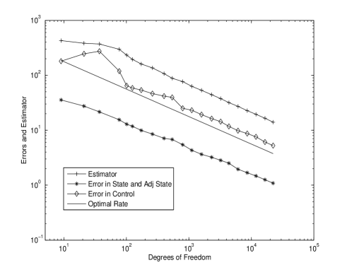
Figure 5.1. Errors and estimator for Example 1

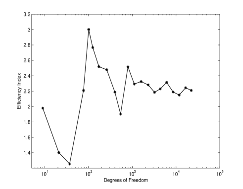
Figure 5.2. Efficiency Index for Example 1

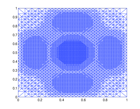
Figure 5.3. Adaptive mesh refinement for Example 1

Example 2. In this example, we test the performance of the a posteriori error estimator for a distributed control problem in the presence of re-entrant corners. The domain $\Omega$ is set to be $L-$shaped as it is shown in Figure 5.5. We set the source term $f=1$ and the observation $u_{d}=1$. In this case since we do not have exact solutions at hand, we test the optimal convergence of the error estimator and its performance in capturing the re-entrant corner. The numerical experiment shows that the error estimator converges optimally (see Figure 5.4) and refines the mesh locally at the reentrant corner (see Figure 5.5) as it should be expected.

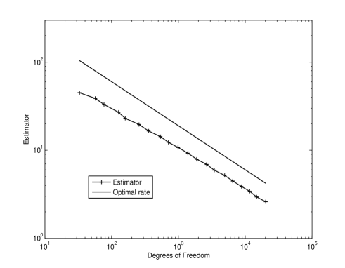
Figure 5.4. Errors and estimator for Example 2

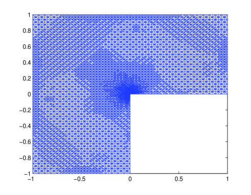
Figure 5.5. Mesh refinement for Example 2

6. Variational discontinuous discretization method

In this section, the variational discretization method (control being not discretized) introduced in [29] will be discussed in the context of discontinuous Galerkin methods and then error estimates will be discussed. For this we use the notation and the setting in Section 3. The variational discontinuous discretization method is defined as to find $(\tilde{u}_{h},\tilde{\phi}_{h},\tilde{q})\in V_{h}\times V_{h}\times Q_{ad}$ such that

(6.1) $$a_{h}(\tilde{u}_{h},v_{h}) =f(v_{h})+\langle\tilde{q},B_{h}v_{h}\rangle\quad\forall v_{h}\in V_{h},\quad$$

(6.2) $$a_{h}(v_{h},\tilde{\phi}_{h}) =(\tilde{u}_{h}-u_{d},v_{h})\quad\forall v_{h}\in V_{h},\quad$$

(6.3) $$\langle B_{h}\tilde{\phi}_{h}+\alpha\tilde{q},p-\tilde{q}\rangle \geq 0\quad\forall p\in Q_{ad},$$

The following lemma is proved in the same lines as that of Lemma 3.1:

Lemma 6.1.

There hold

$$\langle B_{h}(\tilde{\phi}_{h}-P_{h}\phi),q-\tilde{q}\rangle \geq\alpha\|q-\tilde{q}\|_{Q}^{2}+\langle B_{h}(\phi-P_{h}\phi),q-\tilde{q}\rangle.$$

Proof.

From (6.3) and (3.3), we have

$$\langle B_{h}\tilde{\phi}_{h}+\alpha\tilde{q},q-\tilde{q}\rangle \geq 0,$$

$$-\langle B_{h}\phi+\alpha q,q-\tilde{q}\rangle \geq 0,$$

and by adding them, we find

$$\langle B_{h}(\tilde{\phi}_{h}-\phi)+\alpha(\tilde{q}-q),q-\tilde{q}\rangle \geq 0.$$

This implies

$$\langle B_{h}(\tilde{\phi}_{h}-P_{h}\phi),q-\tilde{q}\rangle \geq\alpha\|q-\tilde{q}\|_{Q}^{2}+\langle B_{h}(\phi-P_{h}\phi),q-\tilde{q}\rangle,$$

and hence the proof is completed. ∎

The error estimate for the control and the state are derived in the following theorem.

Theorem 6.2.

There hold

$$\|q-\tilde{q}\|_{Q}+\|u-\tilde{u}_{h}\|_{W}\leq C\left(\|B_{h}(\phi-P_{h}\phi)\|_{Q}+\|u-P_{h}u\|_{W}\right).$$

Proof.

From (6.1)-(6.2) and the definition of $P_{h}$, we have

(6.4) $$a_{h}(P_{h}u-\tilde{u}_{h},v_{h}) =\langle q-\tilde{q},B_{h}v_{h}\rangle\quad\forall v_{h}\in V_{h},$$

(6.5) $$a_{h}(v_{h},P_{h}\phi-\tilde{\phi}_{h}) =(u-\tilde{u}_{h},v_{h})\quad\forall v_{h}\in V_{h}.$$

Take $v_{h}=P_{h}u-\tilde{u}_{h}$ in (6.5), $v_{h}=P_{h}\phi-\tilde{\phi}_{h}$ in (6.4) and subtract the resulting equations to find

$$\langle q-\tilde{q},B_{h}(P_{h}\phi-\tilde{\phi}_{h})\rangle-(u-\tilde{u}_{h},P_{h}u-\tilde{u}_{h})=0.$$

This implies

$$\langle q-\tilde{q},B_{h}(\tilde{\phi}_{h}-P_{h}\phi)\rangle+\|P_{h}u-\tilde{u}_{h}\|_{W}^{2}=(u-P_{h}u,\tilde{u}_{h}-P_{h}u).$$

Using Lemma 6.1, we find

$$\alpha\|q-\tilde{q}\|_{Q}^{2}+\|P_{h}u-\tilde{u}_{h}\|_{W}^{2} \leq-\langle B_{h}(\phi-P_{h}\phi),q-\tilde{q}\rangle+(u-P_{h}u,\tilde{u}_{h}-P_{h}u)$$

$$\leq C\left(\|B_{h}(\phi-P_{h}\phi)\|_{Q}^{2}+\|u-P_{h}u\|_{W}^{2}\right)$$

$$\quad+\frac{1}{2}\|\tilde{u}_{h}-P_{h}u\|_{W}^{2}+\frac{\alpha}{2}\|q-\tilde{q}\|_{Q}^{2}.$$

This completes the proof. ∎

The energy norm error estimates for the state and the adjoint state are proved in the following:

Theorem 6.3.

There hold

$$\|\phi-\tilde{\phi}_{h}\|_{h} \leq C\left(\|\phi-P_{h}\phi\|_{h}+\|B_{h}(\phi-P_{h}\phi)\|_{Q}+\|u-P_{h}u\|_{W}\right),$$

$$\|u-u_{h}\|_{h} \leq C\left(\|u-P_{h}u\|_{h}+\|B_{h}(\phi-P_{h}\phi)\|_{Q}+\|u-P_{h}u\|_{W}\right).$$

Proof.

The estimate in Theorem 6.2, the continuity of $a_{h}$ on $V_{h}$, the error equation (6.5), the assumption (P-T) and the triangle inequality imply

$$\|\phi-\tilde{\phi}_{h}\|_{h} \leq\|\phi-P_{h}\phi\|_{h}+\|P_{h}\phi-\tilde{\phi}_{h}\|$$

$$\leq\|\phi-P_{h}\phi\|_{h}+C\|u-\tilde{u}_{h}\|_{W}$$

$$\leq C\left(\|\phi-P_{h}\phi\|_{h}+\|B_{h}(\phi-P_{h}\phi)\|_{Q}+\|u-P_{h}u\|_{W}\right).$$

The error equation (6.4) and the assumption (3.8) imply

$$a_{h}(P_{h}u-\tilde{u}_{h},P_{h}u-\tilde{u}_{h}) =\langle q-\tilde{q},B_{h}(P_{h}u-\tilde{u}_{h})\rangle$$

$$\leq C\|q-\tilde{q}\|_{Q}\,\|P_{h}u-\tilde{u}_{h}\|_{h}.$$

The rest of the proof follows from Theorem 6.2. ∎

Similarly, we can find a posteriori error estimates in the same lines. In this case the a posteriori error estimator does not involve the term $\|(B_{h}\tilde{\phi}_{h}+\alpha\tilde{q})-\Pi_{h}(B_{h}\tilde{\phi}_{h}+\alpha\tilde{q})\|_{Q}$.

7. Conclusions

We have developed a framework for the error analysis of discontinuous finite element methods for elliptic optimal control problems with control constraints. The abstract analysis provides best approximation results which will be useful in convergence of adaptive methods and delivers a reliable and efficient a posteriori error estimator. The results are applicable to a variety of discontinuous Galerkin methods (including classical nonconforming methods) applied to elliptic optimal control problems (distributed and Neumann) with constraints on control. Applications to $C^{0}$ interior penalty methods for optimal control problems governed by the biharmonic equation with simply supported boundary conditions are established. Numerical experiments illustrate the theoretical findings. Variational discretization method is discussed in the context of discontinuous Galerkin methods and corresponding error estimates are derived.

Acknowledgements: The first author would like to acknowledge the support from NBHM-India, the second author would like to acknowledge the support from DST fast track project and all the authors would like to thank the UGC Center for Advanced Study.

References

- [1] T. Apel, P. Johannes and A. Rösch Finite element error estimates for Neumann boundary control problems on graded meshes. Comput. Optim. Appl., 52:3–28, 2012.
- [2] S. Badia, R. Codina, T. Gudi and J. Guzman. Error analysis of discontinuous Galerkin methods for Stokes problem under minimal regularity. IMA J. Numer. Anal., 34:800-819, 2014.
- [3] H. Blum and R. Rannacher. On the boundary value problem of the biharmonic operator on domains with angular corners. Math. Methods Appl. Sci., 2:556–581, 1980.
- [4] S.C. Brenner, K. Wang and J. Zhao. Poincaré-Friedrichs inequalities for piecewise functions. Numer. Funct. Anal. Optim., 25: 463-478, 2004.
- [5] S.C. Brenner and L.-Y. Sung. interior penalty methods for fourth order elliptic boundary value problems on polygonal domains. J. Sci. Comput., 22/23:83–118, 2005.
- [6] S.C. Brenner and L.R. Scott. The Mathematical Theory of Finite Element Methods Third Edition. Springer-Verlag, New York, 2008.
- [7] S.C. Brenner, T. Gudi and L.-Y. Sung. An a posteriori error estimator for a quadratic interior penalty method for the biharmonic problem. IMA J. Numer. Anal., 30 (2010), pp. 777 – 798.
- [8] S.C. Brenner, S. Gu, T. Gudi and L.-Y. Sung. A quadratic interior penalty method for linear fourth order boundary value problems with boundary conditions of the Cahn-Hilliard type. SIAM J. Numer. Anal., 50:2088-2110, 2012.
- [9] S.C. Brenner and M. Neilan. A interior penalty method for a fourth order elliptic singular perturbation problem. SIAM J. Numer. Anal., 49:869–892, 2011.
- [10] W. Cao and D. Yang. Ciarlet-Raviart mixed finite element approximation for an optimal control problem governed by the first bi-harmonic equation. Journal of Computational and Applied Mathematics, 233:372–388, 2009.
- [11] C. Carstensen, D. Gallistl and M. Schedensack. Discrete reliability of Crouzeix-Raviart FEMs. SIAM J. Numer. Anal., 51:2935-2955, 2013.
- [12] E. Casas and J. P. Raymond. Error estimates for the numerical approximation of dirichlet boundary control for semilinear elliptic equations. SIAM J. Control Optim., 45:1586-1611, 2006.
- [13] P.G. Ciarlet. The Finite Element Method for Elliptic Problems. North-Holland, Amsterdam, 1978.
- [14] K. Deckelnick and M. Hinze. Convergence of a finite element approximation to a state-constrained elliptic control problem. SIAM J. Numer. Anal., 45: 1937-1953, 2007.
- [15] K. Deckelnick, A. Günther and M. Hinze. Finite Element Approximation of Dirichlet Boundary Control for Elliptic PDEs on Two- and Three-Dimensional Curved Domains. SIAM J. Numer. Anal., 48:2798-2819, (2009).
- [16] W. Dörlfer. A convergent adaptive algorithm for Poisson’s equation. SIAM J. Numer. Anal., 33:1106–1124, 1996.
- [17] G. Engel, K. Garikipati, T.J.R. Hughes, M.G. Larson, L. Mazzei, and R.L. Taylor. Continuous/discontinuous finite element approximations of fourth order elliptic problems in structural and continuum mechanics with applications to thin beams and plates, and strain gradient elasticity. Comput. Methods Appl. Mech. Engrg., 191:3669–3750, 2002.
- [18] S. Frei, R. Rannacher and W. Wollner, A priori error estimates for the finite element discretization of optimal distributed control problems governed by the biharmonic operator, Calcolo, online first (2012) doi:10.1007/s10092-012-0063-3.
- [19] T. Geveci. On the approximation of the solution of an optimal control problems governed by an elliptic equation., M2AN., 13:313–328, 1979.
- [20] P. Grisvard. Elliptic Problems in Nonsmooth Domains. Pitman, Boston, 1985.
- [21] P. Grisvard. Singularities In Boundary Value Problems. Springer, 1992.
- [22] T. Gudi. A new error analysis for discontinuous finite element methods for linear elliptic problems. Math. Comp., 79 (2010), pp. 2169 – 2189.
- [23] T. Gudi and M. Neilan. An interior penalty method for a sixth order elliptic problem. IMA J. Numer. Anal., 31:1734–1753, 2011.
- [24] T. Gudi, N. Nataraj and K. Porwal. An interior penalty method for distributed optimal control problems governed by the biharmonic operator. Comput. Math. Appl., to appear. doi: 10.1016/j.camwa.2014.08.012.
- [25] A. Günther and M. Hinze. Elliptic control problems with gradient constraints variational discrete versus piecewise constant controls Comput. Optim. Appl., 40:549–566, 2011.
- [26] M. D. Gunzburger, L. S. Hou, T. Swobodny. Analysis and finite element approximation of optimal control problems for the stationary Navier Stokes equations with Dirichlet controls. Math. Model. Numer. Anal., 25:711 -748, 1991.
- [27] R. Falk. Approximation of a class of optimal control problems with order of convergence estimates. J. Math. Anal. Appl., 44:28–47, 1973.
- [28] M. Hintermller, K. Ito and K. Kunish. The primal-dual active set strategy as a semismooth Newton method. SIAM J. Optim., 13:865–888, 2003.
- [29] M. Hinze. A variational discretization concept in control constrained optimization: The linear-quadratic case. Comput. Optim. Appl., 30:45–61, 2005.
- [30] M. Hintermüller, R. H. W. Hoppe, Y. Iliash and M. Kiewag. An a posteriori error analysis of adaptive finite element methods for distributed elliptic control problems with control constraints., ESAIM: Control, Optimisation and Calculus of Variations, 14: 540–560, 2008.
- [31] J. Hu, Z. C. Shi, and J. Xu. Convergence and optimality of the adaptive Morley element method. Numer. Math., 121:731–752, 2012.
- [32] G. Kanshat and N. Sharma. Divergence-conforming Galerkin methods and interior penalty method. SIAM J. Numer. Anal., 52: 1822-1842, 2014.
- [33] K. Kohls, A. Rösch and K. Siebert. A posteriori error analysis of optimal control problems with control constraints. SIAM J. Control & Optimization 52(3):1832-1861, 2014.
- [34] S. May, R. Rannacher, and B. Vexler. Error analysis for a finite element approximation of elliptic dirichlet boundary control problems. SIAM J. Control Optim., 51:2585-2611, 2013.
- [35] C. Meyer and A. Rösch, Superconvergence properties of optimal control problems, SIAM J. Control & Optimization 3(43) : 970-985, 2004.
- [36] G. Of, T. X. Phan, O. Steinbach. An energy space finite element approach for elliptic Dirichlet boundary control problems. Numer. Math., doi:10.1007/s00211-014-0653-x, 2014.
- [37] C. Ortner and W. Wollner. A priori error estimates for optimal control problems with pointwise constraints on the gradient of the state. Numer. Math., 118: 587–600, 2011.
- [38] F. Tröltzsch, Optimale Steuerung Partieller Differentialgleichungen, I edn. Vieweg, Cambridge University Press 2005.