Modeling the emergence of polarity patterns for the intercellular transport of auxin in plants

Abstract

The hormone auxin is actively transported throughout plants via protein machineries including the dedicated transporter known as PIN. The associated transport is ordered with nearby cells driving auxin flux in similar directions. Here we provide a model of both the auxin transport and of the dynamics of cellular polarisation based on flux sensing. Our main findings are: (i) spontaneous intracellular PIN polarisation arises if PIN recycling dynamics are sufficiently non-linear, (ii) there is no need for an auxin concentration gradient, and (iii) ordered multi-cellular patterns of PIN polarisation are favored by molecular noise.

Keywords: PIN polarity, auxin transport, reaction-diffusion systems

I Introduction

In plants, the initiation of different organs such as roots, leaves or flowers depends on the cues received by cells, be they from the environment or signals produced by the plant itself scheres2001 . Amongst these signals, the hormone auxin plays a central role. Auxin was discovered over a half century ago along with some of its macroscopic effects on leaf and root growth went . It is actively transported throughout the whole plant and it is a major driver of the plant’s architecture reinhardt2000 ; reinhardt2003 .

In the past decade, much has been learned about the molecular actors controlling auxin movement. First, cell-to-cell auxin fluxes depend on two classes of transporters palme1999 ; muday2001 ; petrasek2009 : (i) PIN, (for ‘PIN-FORMED”), that pumps auxin from inside to outside cells galweiler1998 , and (ii) AUX1, (for ‘AUXIN RESISTANT 1”), which pumps auxin from outside to inside cells. Second, auxin accumulation drives cell proliferation and differentiation. Third, cells are polarized in terms of their PIN content, that is PIN transporters localize mainly to one side of cells traas2013 . In addition, these polarizations are similar from cell to cell so that auxin is systematically transported along the direction of this polarization. That ordering has major consequences for the growth and morphogenesis of the plant because it affects the distribution of auxin, and auxin drives both organ growth and the initiation of new organs auxinbook ; pinbook . Much work has focused on how PIN polarization patterns lead to auxin distributions, but two major questions remain unanswered concerning the emergence of PIN polarization patterns: (i) How can PIN become polarized in cells in the absence of auxin gradients? (ii) Can PIN polarization patterns be coherent on the scale of many cells?

To address these questions, we take a modeling approach here, incorporating the main ingredients of what is currently known about (i) intercellular auxin transport and (ii) intracellular PIN dynamics. We will first provide a deterministic framework using differential equations for modeling the dynamics of auxin and of PIN cellular polarization. Our model exhibits multiple steady states that we characterize, the simplest ones being translation-invariant with all cells having the same PIN polarization. We find that the emergence of polarization depends on the degree of non-linearity within the PIN recycling dynamics. We then include molecular noise in this system coming from the stochastic dynamics of PIN intra-cellular localization. Interestingly, for biologically realistic values of the parameters of the model, the system is driven into a state where cells coherently polarize in the same direction. In effect, the noise selects a robust self-organised state having homogeneous PIN polarization, corresponding to a noise-induced ordering scenario.

II The model of auxin dynamics and PIN recycling

Auxin transport in plants is typically organized in sheets, each sheet consisting of a single layer of cells. For instance in the case of the tips of shoots, almost all the transport arises in a single cell sheet which is referred to as the L1 layer dereuille2006 ; buylla2010 ; vernoux2010 ; smith2006 ; jonsson2006 . For our model, we shall therefore work with one layer of cells. We start with a lattice of cubic cells having edges of length $\Lambda$ separated by apoplasts – the space between two adjacent cells – of width $\lambda$ (cf. Fig. 1 which represents a view from above of this system). Tissues consist of closely packed cells so $\lambda\ll\Lambda$; typical values are $\lambda\approx 1\mu m$ and $\Lambda\approx 20\mu m$. The hormone auxin reinhardt2000 is subject to different processes:

• production and degradation inside cells, with rate constants $\beta~{}$ and $\rho$;

• passive diffusion within cells, within apoplasts, and also between cells and apoplasts;

• active transport across cell membranes via transporters.

Since cell membranes form barriers to exchanges of molecules, taking a molecular species from one side to the other often requires dedicated transporters. In the case of auxin, the cell membrane does allow some amount of diffusion of the hormone but much less than the inside of the cell or of the apoplast where diffusion is very rapid. We call $D$ the associated diffusion constant (measured in $\mu\text{m}^{2}/\text{s}$) within the membrane of thickness $\epsilon$ whereas formally we consider diffusion inside cells and inside apoplasts to arise infinitely quickly; as a consequence, intra-cellular variations of auxin concentration are negligible and so are those within an apoplast. In addition, auxin is subject to active processes that transport it across the cell membrane. Experimental evidence has shown that there are different molecular transporters for the in-going and out-going fluxes, transporters called respectively AUX1 and PIN reinhardt2003 ; friml2006 . These transporters are normally localised on the cell membrane where they can play their role to actively transport auxin between the inside and the outside of the cell. The out-going transporters belong to a large family whose members specialize to different organs and tissues of the plant krecek2009 : in our context, we will refer to these transporters simply as PIN paponov2005 .

The dynamics of auxin concentration in each region (cell or apoplast) is specified by the trans-membrane flux densities of auxin ($\phi_{AUX1}$ and $\phi_{PIN}$ for the active transport and a diffusion contribution proportional to the diffusion constant $D$) along with production and degradation terms. In the case of cells, we have

$$\begin{split}\frac{dA_{c}(P,t)}{dt}&=\beta~{}-\rho A_{c}(P,t)+\Lambda^{-1}\sum_{P^{\prime}}[\phi_{AUX1}(P,P^{\prime},t)-\phi_{PIN}(P,P^{\prime},t)+D(A_{a}(P,P^{\prime},t)-A_{c}(P,t))/\epsilon].\end{split}$$ (1)

In this equation, $A_{c}(P,t)$ is the auxin intra-cellular concentration of the cell centered at position $P=(x,y)$ at time $t$, and $A_{a}(P,P^{\prime},t)$ is the auxin concentration in the apoplast separating nearest neighbor cells $P$ and $P^{\prime}$. Both concentrations will be specified in micro-moles per liter ($\mu$M for micro-molar). Furthermore, only the diffusion constant of auxin within the cell membrane appears because it is far smaller than that within a cell or apoplast; note that the flux is proportional to the gradient, thus the factor $D/\epsilon$ where $\epsilon$ is the thickness of the membrane. $\phi_{AUX1}(P,P^{\prime},t)$ and $\phi_{PIN}(P,P^{\prime},t)$ are the auxin flux densities carried by the transporters through the corresponding “face” of cell $P$, i.e., the area of the membrane of cell $P$ that faces cell $P^{\prime}$. By convention, the sign of each flux is positive, the one for PIN going from the inside to the outside of the cell, and the one for AUX1 going from outside to inside. These flux densities have units of micro-moles per second per surface area ($\mu m^{2}$). The sum over cells $P^{\prime}$ is restricted to the neighbors of $P$ so in effect one sums over all sides of the cell $P$ under consideration that connect it to the rest of the system. The parameters $\beta$ and $\rho$ are the rates of auxin production and degradation. In addition, the division by the factor $\Lambda$ (the width of a cell) appears because one goes from flux densities to effects on the concentrations inside cells. Lastly, in our framework as depicted in Fig. 1, apoplasts connect only to cells and vice versa, so there are neither cell-to-cell nor apoplast-to-apoplast contacts.

In a similar fashion, the concentration $A_{a}(P,P^{\prime},t)$ of auxin in the apoplast (of thickness $\lambda$) separating cells $P$ and $P^{\prime}$ obeys the differential equation:

$$\begin{split}\frac{dA_{a}(P,P^{\prime},t)}{dt}&=\lambda^{-1}[\phi_{PIN}(P,P^{\prime},t)-\phi_{AUX1}(P,P^{\prime},t)+\phi_{PIN}(P^{\prime},P,t)-\phi_{AUX1}(P^{\prime},P,t)+\\ &+D(A_{c}(P,t)+A_{c}(P^{\prime},t)-2A_{a}(P,P^{\prime},t))/\epsilon]~{}.\end{split}$$ (2)

Note that there is neither production nor degradation of auxin in the apoplast (it is a passive medium and auxin has a long lifetime in the absence of the active degradation processes present in cells).

In Arabidopsis, which currently is the most studied plant, propensity of AUX1 influx transporters seems to be several times higher than that of passive diffusion kramer2006 ; kramer2008 , thus active processes are probably the main drivers of auxin distribution. Furthermore, the transporters AUX1 and PIN are believed to be completely unidirectional; the associated molecular mechanisms are unclear but involve first the binding of auxin and then conformational changes. Because these processes are analogous to enzymatic reactions, we model the associated auxin fluxes via irreversible Michaelis-Menten kinetics:

$$\phi_{AUX1}(P,P^{\prime},t)=\frac{N^{AUX1}}{\Lambda^{2}}\cdot\alpha\cdot\frac{A_{a}(P,P^{\prime},t)}{1+\frac{A_{a}(P,P^{\prime},t)}{A^{*}}+\frac{A_{c}(P,t)}{A^{**}}},$$ (3)

$$\phi_{PIN}(P,P^{\prime},t)=\frac{N^{PIN}}{\Lambda^{2}}\cdot\gamma\cdot\frac{A_{c}(P,t)}{1+\frac{A_{a}(P,P^{\prime},t)}{A^{*}}+\frac{A_{c}(P,t)}{A^{**}}},$$ (4)

where $\alpha$ and $\gamma$ are kinetic constants analogous to catalysis rates. The factor $\Lambda^{2}$ on the right-hand side of these equations corresponds to the surface of the face of each cell, and connects the flux density to the (absolute) flux. At a molecular level, $N^{AUX1}$ (respectively $N^{PIN}$) refers to the number of AUX1 (respectively PIN) transporters on the area of $P$’s membrane which faces cell $P^{\prime}$. Finally, $A^{*}$ and $A^{**}$ play the role of Michaelis-Menten constants associated with saturation effects; these could have been taken to be different in Eqs. 3 and 4 without any qualitative consequences for the behavior of the model.

We are not aware of any experimental evidence that the distribution of AUX1 transporters changes with time or that these transporters contribute to cell polarity. Thus we shall assume that their numbers are constant on each face of the cell. In contrast, PIN transporters are particularly important for driving morphogenesis through the formation of polarity patterns. Often they define clearly polarized fields in tissues dereuille2006 ; sassi2013 where cells see their PINs predominantly localised to one of their faces, with the specific face being the same for many cells. That polarity leads to coherent auxin transport, even on the scale of the whole plant, allowing in particular auxin to be transported from shoots to rootsfriml2006-2 ; benkova2003 . To take into account this possibility of intracellular polarization of PIN, we introduce the four faces of a cell as $N$ for north, $S$ for south, $E$ for east and $W$ for west. (The two faces parallel to the sheet play no role in our simplified model involving a single layer of cells.) Then each face of a cell has a potentially variable number of PIN transporters:

$N_{f}^{PIN}$,   $f=N,S,E,W$.

Furthermore we impose the constraint $\sum_{f}N_{f}^{PIN}\equiv\sigma$, a cell-independent constant so each cell has the same number of PIN transporters at all times.

The dynamics of PIN seem complex: it is known that PINs are subject to “recycling” within a cell through different mechanisms including transport from the membrane to the Golgi apparatus and back to the membrane petrasek2009 ; lofke2013 ; tanaka2013 ; kleinevehn2011 . Most modeling takes PIN dynamics to be driven by surrounding auxin concentrations vanberkel2013 ; kramer2008 ; kramer2006 ; smith2006 ; jonsson2006 ; wabnik2010 . For instance it has been postulated that PIN might accumulate to the membrane facing the neighboring cell with the highest concentration of auxin smith2006 ; jonsson2006 . As a consequence, the presence of an auxin gradient becomes a necessary condition for PIN polarization. Here we consider instead dynamics based on flux sensing where PIN recycling rates are modulated by the amount of auxin flux transported by those same PIN transporters. Mathematically, we take the PIN dynamics on a face $f$ ($f=N,S,E,W$) of a cell to be specified by a Hill equation of exponent $h$:

$$\begin{split}\frac{dN_{f}^{PIN}}{dt}&=-\frac{3}{4\tau}N_{f}^{PIN}\frac{1}{1+\bigg{(}\frac{\phi_{f}^{PIN}}{\phi^{*}}\bigg{)}^{h}}+\frac{1}{4\tau}\sum_{f^{\prime}}N_{f^{\prime}}^{PIN}\frac{1}{1+\bigg{(}\frac{\phi_{f^{\prime}}^{PIN}}{\phi^{*}}\bigg{)}^{h}}.\end{split}$$ (5)

Note that PINs are treated here as continuous variables because in the following the number of molecules is high so such an approximation is appropriate. Nevertheless, later we shall treat the actual numbers via our stochastic model. The above differential equations model the competitive recycling of the PINs amongst the faces of a given cell in a flux dependent manner. Note that $\tau$ is the characteristic time scale of the recycling process and that the dynamics enforce the constraint of conservation of the total number of PIN transporters inside each cell. Also, in Eq. 5, $\phi_{f}^{PIN}$ is the flux density through face $f$ while $\phi^{*}$ is a Michaelis-Menten-like constant.

To understand the consequences of Eq. 5, consider first the low flux limit, $\phi_{f}^{PIN}$ being small for all faces, so that all denominators can be ignored. At a molecular level, each transporter leaves the cell membrane at a rate proportional to $\tau^{-1}$; transporters are then brought into the cytoplasm or Golgi apparatus; finally they get reallocated randomly to any of the 4 faces. In such a low flux regime, cells will show no PIN polarization. Second, consider instead the case where for at least one face $f$, $\phi_{f}^{PIN}/\phi^{*}$ is large. That face will benefit from the recycling, recruiting more transporters from the other faces than it loses. ($\phi^{*}$ is just the scale at which flux sensing in this system becomes important). At an individual transporter level, the competitive recycling means that transporters which are actively shuttling auxin see their rate of recycling go down. How this happens depends on unknown molecular details, nevertheless, the rate of detachment of a transporter from the membrane probably depends on what fraction of the time it is binding auxin and thus the rate of detachment will show a dependence on $\phi_{f}^{PIN}$. One may attempt to model this via a simple hyperbolic law to describe saturation effects. To be more general, we have introduced a Hill exponent, $h$, into the dynamics as given in Eq. 5. Such a functional form is often used in the kinetic modeling of binding processes; in that framework, $h$ is an integer related to the number of molecules that must co-localize, and as such, it reflects co-operative effects. In the absence of detailed knowledge of the molecular mechanisms controlling PIN recycling, we use this phenomenological form where $h$ is associated with the non-linearity of the PIN recycling dynamics and we will see whether or not $h$ plays an important role. In the Supplementary Material, we will see that our conclusions are insensitive to the precise form of the equations describing PIN recycling by replacing the Hill form with a stretched exponential.

Figure 1: (a) Schematic two-dimensional view of the system consisting of a single layer of cells. Cubic cells of size $\Lambda$ are in orange, apoplasts of width $\lambda$ are in white. On the right: a zoom on two neighboring cells. Gray circles stand for auxin and red arrows represent the incoming AUX1 mediated fluxes in cells, while light blue arrows represent the outgoing PIN mediated fluxes. In these views from above, the thickness ($\Lambda$) of the cells is not shown. (b) Role of transmembrane transporters. PINs pump auxin from the inside of the cell to an adjacent apoplast. AUX1 plays the reverse role, pumping auxin from apoplasts to the inside of the cell. Dashed arrows within a cell illustrate PIN recycling.

The model is now completely specified and involves the 15 parameters $\Lambda$, $\lambda$, $\epsilon$, $\alpha$, $\beta~{}$, $\gamma$, $\rho$, $A^{*}$, $A^{**}$, $\phi^{*}$, $\tau$, $\sigma$, $N^{AUX1}$, $D$, and $h$. Some of these parameters can be absorbed in scale changes. Nevertheless, to keep the physical interpretation as transparent as possible, we stay with the dimensional form of the equations. Whenever possible, we assign values to the parameters using published estimates or compilations thereof Deinum_Thesis ; kramer2006 ; kramer2008 . For instance, mass-spectrometry measurements ljung2001 in very young leaves quantify the concentration of auxin to be about 250 picograms per milligram of tissue. Since the molecular mass of auxin is about 175 Da, $A_{c}$ is of the order of 1 micro-molar. As we shall see, in the steady-state regime, $\beta/\rho=A_{c}$, a relation providing a constraint on those two parameters. Furthermore, a direct estimate of $\beta$ follows from isotopic labeling measurements ljung2001 which show that biosynthesis replenishes auxin within about one day; we have thus set $\beta$=1/day. Radioactive labeling has also provided estimates for mean displacement velocities of auxin kramer2006 ; kramer2008 which we have used to constrain the parameters $\alpha$ and $\gamma$. Unfortunately, for other parameters (and in particular the Michaelis-Menten constants) no direct or indirect estimations from experimental data are available. For most such cases, we use ball-park estimations that seem reasonable, for instance a hundred PIN molecules seems like a too low number while $10^{4}$ is perhaps on the high side. However, for $h$, which provides a phenomenological parameterization of non-linear effects in PIN recycling, we have little choice but to study the behavior of the model as a function of its value. We use the same strategy for $D$. Thus, both $D$ and $h$ will be used as control parameters, allowing us to map out a two-dimensional phase diagram. For instance, when increasing $D$, passive diffusion will overcome the effects of active transport, allowing one to probe the importance of active vs. passive transport in the establishment of PIN polarization. Unless specified otherwise, all other parameter values are set as provided in Table 1.

$\beta~{}$	1 $\mu$M $\cdot$ day-1
$\rho$	1 day-1
$\alpha$	0.1 L $\cdot$ s-1
$\gamma$	$10^{-4}$ L $\cdot$ s-1
$A^{*}$	2 $\times 10^{-3}$ $\mu$M
$A^{**}$	0.8 $\mu$M
$\phi^{*}$	4 $\times 10^{-6}$ moles $\cdot$ $\mu$m-2 s-1
$N^{AUX1}$	200 per face
$\sigma$	1000
$\Lambda$	20 $\mu$m
$\lambda$	1 $\mu$m
$\epsilon$	10 nm
$\tau,\tau_{1D}$	30 min

Table 1: Parameters used in the model. M stands for molarity, i.e., number of moles per liter. L stands for liter.

Since our aim is to understand how ordered polarity patterns arise in a system described by this model, it is appropriate to define an order parameter to quantify the ordering of flux directions or PIN intra-cellular localisation. We thus introduce the two-dimensional polarization vector $\vec{\delta}$ for a cell at position $P=(x,y)$; its components depend on the face-to-face difference of the number of PINs along each direction (say horizontal or vertical) in the following way:

$$\vec{\delta}(x,y)\equiv\begin{cases}\delta_{1}(P)=\frac{N_{E}^{PIN}(P)-N_{W}^{PIN}(P)}{\sigma}\\ \\ \delta_{2}(P)=\frac{N_{N}^{PIN}(P)-N_{S}^{PIN}(P)}{\sigma}\end{cases}$$ (6)

The vector in Eq. 6 has a length $|\vec{\delta}(P)|\in[0,1]$: the two extreme values represent respectively the unpolarized case, i.e., $N_{f}^{PIN}=\sigma/4$ for all $f$, and the fully polarized case, i.e., $N_{f}^{PIN}=\sigma$ for one face while $N_{f}^{PIN}=0$ for all other faces. Individual components can vary in $[-1,1]$ and the extreme points give the maximum polarization in one direction or the other.

A first step will consist in understanding the behavior of this system in a one-dimensional framework.

III Analysis of the one-dimensional model

III.1 Dynamical equations

Let us replace the square lattice represented in Fig. 1 by a row of cubic cells forming a one-dimensional lattice. As before, between two adjacent cells there is exactly one apoplast. In this one-dimensional model, all diffusion and transport is horizontal and PIN is defined only on the left (West) and right (East) face of each cell. The dynamics of $A_{c}$ and $A_{a}$ in each cell are obtained from Eqs. 1 and 2 by setting the vertical fluxes to 0. Given the constraint of conservation of total PIN transporters in each cell and the fact that only two faces contribute, the dynamics of PIN numbers are completely determined via the dynamics of $N^{PIN}_{E}$ and there is just one independent equation for each cell:

$$\frac{dN^{PIN}_{E}}{dt}=-\frac{1}{\tau_{1D}}N^{PIN}_{E}\frac{1}{1+(\frac{\phi^{PIN}_{E}}{\phi^{*}})^{h}}+\frac{1}{\tau_{1D}}N^{PIN}_{W}\frac{1}{1+(\frac{\phi^{PIN}_{W}}{{\phi^{*}}})^{h}}$$ (7)

where $\tau_{1D}=4\tau/3$ and $N^{PIN}_{W}=\sigma-N^{PIN}_{E}$ . Furthermore, polarization is no longer a vector but a scalar, given by the first component of Eq. 6. It varies in $[-1,1]$: when $\delta(x)\approx-1$, almost all the PINs are on the left-hand side of the cell, while when $\delta(x)\approx 1$ they are almost all on the right-hand side.

III.2 Steady-state auxin concentrations given translation-invariant PIN configurations

Assuming periodic boundary conditions, the row of cells becomes a ring; this idealization is convenient for the mathematical and phase diagram analysis. Consider the steady-state solutions of the differential equations. With periodic boundary conditions, one expects some steady states to be translationally invariant. In that situation, all quantities are identical from cell to cell and from apoplast to apoplast. We can then drop all time and spatial dependence in the variables, e.g., $A_{c}(P,t)=A_{c}$ for all $P$ and $t$.

We consider here an arbitrary translation-invariant configuration of PIN transporters (steady-state or not), which implies that the auxin equations will depend only on the total number of transporters per cell. One then has the following equations for steady-state auxin concentrations:

$$\left\{\begin{array}[]{l}0=\beta~{}-\rho A_{c}+\frac{2D}{\Lambda\epsilon}(A_{a}-A_{c})+\frac{2\alpha}{\Lambda^{3}}N^{AUX1}\frac{A_{a}}{1+\frac{A_{a}}{A^{*}}+\frac{A_{c}}{A^{**}}}-\frac{\gamma}{\Lambda^{3}}\sigma\frac{A_{c}}{1+\frac{A_{a}}{A^{*}}+\frac{A_{c}}{A^{**}}}\\ \\ 0=\frac{2D}{\lambda\epsilon}(A_{c}-A_{a})-\frac{2\alpha}{\lambda\Lambda^{2}}N^{AUX1}\frac{A_{a}}{1+\frac{A_{a}}{A^{*}}+\frac{A_{c}}{A^{**}}}+\frac{\gamma}{\lambda\Lambda^{2}}\sigma\frac{A_{c}}{1+\frac{A_{a}}{A^{*}}+\frac{A_{c}}{A^{**}}}\\ \end{array}\right..$$ (8)

These two equations determine $A_{c}$ and $A_{a}$. One can first solve for $A_{c}$ by noting that in apoplasts there is no source or degradation of auxin, thus in the steady state the total flux (transport and diffusion counted algebraically) through an apoplast vanishes and so the same holds for cells. Therefore within cells auxin degradation must compensate exactly auxin production, leading to $\beta-\rho A_{c}=0$. This result, namely $A_{c}=\beta/\rho$, is independent of all other parameters and in particular of the PIN polarization and of $D$ as illustrated in Fig. 2. Furthermore, with $A_{c}$ determined in this way the two equations become equivalent and can be solved for $A_{a}$.

Experimental evidence kramer2006 ; kramer2008 suggests that active transport dominates passive (diffusive) transport in Arabidopsis. Thus the biologically relevant regime probably corresponds to $D$ small. In the low diffusion limit ($D\to 0$), the last equation shows that $A_{a}$ goes to a limiting value that is strictly positive.(A zoom of Fig. 2 would also show this is the case.) Solving this equation using the values of the parameters in Table 1, one finds that the concentration of auxin in cells is much greater than that in apoplasts because $2N^{AUX1}\alpha\gg\sigma\gamma$, i.e., auxin molecules are more easily transported by AUX1 than by PIN (cf. the left limit in Fig. 2). One may also consider what happens when diffusion is important; clearly as $D\to\infty$, the transporters become irrelevant and the equations immediately show that $A_{c}$ and $A_{a}$ become equal. The overall behavior is displayed in Fig. 2.

Figure 2: Auxin steady-state concentrations (red for apoplasts and blue for cells) in an arbitrary PIN translation-invariant configuration as a function of the diffusion constant $D$ in $\mu\text{m}^{2}/\text{s}$. The other relevant model parameters are given in Table 1.

III.3 Translation-invariant dynamics of PIN in the quasi-equilibrium limit for auxin

Microscopic molecular events associated with auxin transport (be they active or passive) arise on very short time scales whereas the PIN recycling requires major cellular machinery and so arises on much longer time scales. Let us therefore take the quasi-equilibrium limit where auxin concentrations take on their steady-state values $A_{c}$ and $A_{a}$. Consider now the dynamical equation for $\delta$, the PIN polarization. Since it involves a single variable, it can always be written as gradient descent relaxational dynamics, i.e., there exists a function $\mathcal{F}(\delta)$ such that:

$$\frac{d\delta}{dt}=-\frac{1}{\tau_{1D}}\frac{d\mathcal{F}(\delta)}{d\delta}.$$ (9)

$\mathcal{F}(\delta)$ plays the role of an effective potential. $\mathcal{F}(\delta)$ is minus the integral of a known function of $\delta$; this integral can be obtained in closed form in terms of hypergeometric functions (see Supplementary Material).

The extrema of $\mathcal{F}$ correspond to steady states for the PIN dynamics, i.e., $d\delta/dt=0$. Maxima are unstable and minima are stable. Thus it is of interest to map out the form of $\mathcal{F}$ as a function of the parameter values. Take for instance $h=2$. Starting with a large value for $D$, use of Mathematica shows that $\mathcal{F}$ has a single global minimum, corresponding to the unpolarized steady state, $\delta=0$. Then as $D$ is lowered, (the Mathematica code of the Supplementary Material provides the user with a knob to change $D$), $\mathcal{F}$ takes on a double-well shape, symmetric about the zero polarization abscissa where the curvature is now negative. At the same time, two new local minima appear at $\pm\delta^{*}$. Thus as $D$ is lowered, the unpolarized state becomes unstable while two new stable steady states of polarization $\pm\delta^{*}$ appear; this situation is illustrated in Fig. 3. If we had used instead $h=0.5$, we would have found no regime in $D$ where $\mathcal{F}$ has the double-well structure: there, the only steady state is the unpolarized one.

Figure 3: Effective potential as a function of the polarization $\delta$ for $D>D_{c}$ (purple) and $D<D_{c}$ (blue) rescaled with $\sigma^{2}$. $h=2$, other parameter values are given in Table 1.

Within this framework, it is possible to determine a critical point $D_{c}$, i.e., a threshold value of the diffusion constant, below which spontaneous symmetry breaking sets in. The value of $D_{c}$ is obtained from the following condition (see also Supplementary Material):

$$\frac{\partial^{2}\mathcal{F}}{\partial\delta^{2}}|_{\delta=0}=0.$$ (10)

In particular, for $h=2$, this leads to a critical value $D_{c}\approx 9.4\times 10^{-7}\mu\text{m}^{2}/\text{s}$. This overall framework provides a convenient intuitive picture for PIN dynamics.

III.4 Spontaneous symmetry breaking and phase diagram for translation-invariant steady states

The previous formalism is complicated because of the form of $\mathcal{F}$. However if one is only interested in the steady states and one does not care about relaxational dynamics, the steady-state equation to solve is relatively simple (cf. Eq. 7 where the left-hand side must be set to 0). We assume as before that $N_{E}^{PIN}$ is translation invariant but also that it is subject to PIN recycling. Since $A_{c}$ and $A_{a}$ in steady states have been previously calculated, all quantities in Eq. 7 are known except for $N_{E}^{PIN}$; it is enough then to solve the associated non-linear equation (we have used Mathematica for this purpose). At given $h$ not too small, we find a transition from polarized to unpolarized states as $D$ crosses the threshold $D_{c}$ (see Fig. 4a which illustrates the case $h=2$).

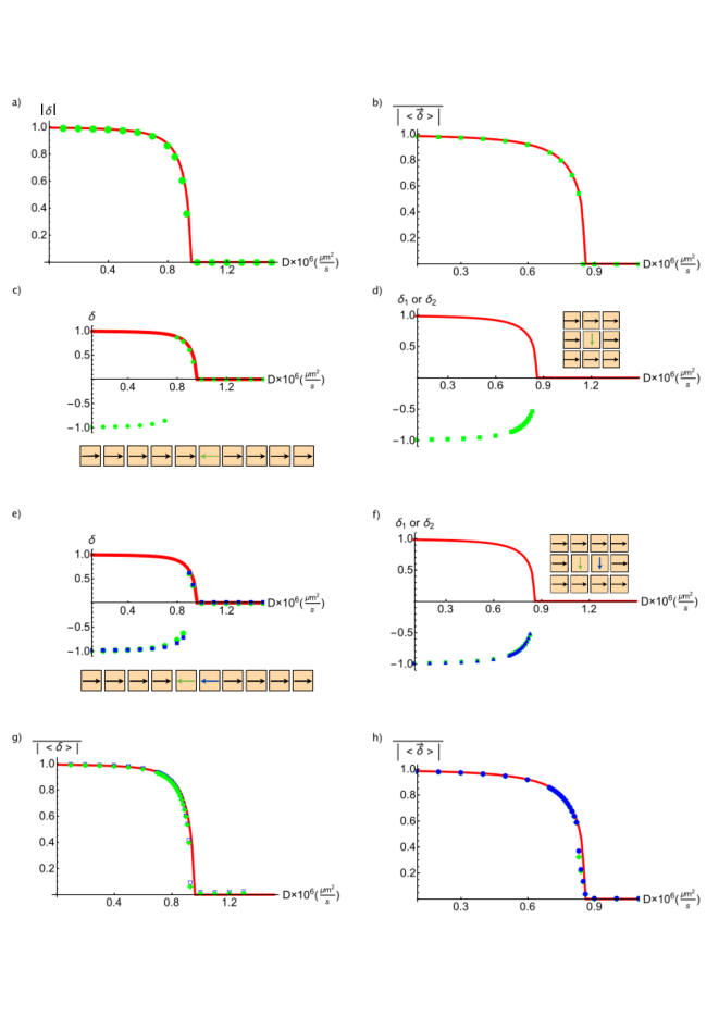
Figure 4:

Figure 4: a) and b) Absolute value of the (translation-invariant) PIN polarization as a function of the diffusion constant $D$ in $\mu\text{m}^{2}/\text{s}$ in steady states respectively for the 1D and the 2D models. Red line: analytical result obtained using Mathematica. Green circles: results of simulating the dynamics of the model containing respectively 20 cells on a ring and 20$\times$20 cells on a lattice until a steady state was reached; a fourth-order Runge-Kutta algorithm numericalrecipes was used and starting configurations were randomized but had positive local PIN polarizations. c),e),d),f) PIN polarization at a defect (green and blue) and in the absence of a defect (red) for a ring of 20 cells as a function of $D$ for the 1D case (c) and e)) and a lattice of 20$\times$20 cells for the 2D case (d) and f)). Drawings (below and insets): initial orientation of PIN polarizations; the green and blue arrows represent the defects. g) and h) Absolute value of the mean PIN polarization per site, averaged over time, as a function of the diffusion constant for the stochastic model for three different ring/lattice sizes (in g), $N_{cells}=20$ green diamonds, $N_{cells}=10$ blue squares, while in h) $N_{cells}=5$ blue circles, $N_{cells}=10$ green diamonds) and for the deterministic model (red line). Simulations were performed using cells on a ring/lattice. $D_{c}$ is slightly lower when using stochastic dynamics. In all the plots, $h=2$ while other parameter values are given in Table 1. In g), $\tau=1$s.

The position of the threshold depends on $h$. However, if $h$ is too small, the transition point disappears, and there are no longer any polarized steady states. To illustrate the situation, consider fixing $D$ to a small value, say $D=10^{-7}\mu\text{m}^{2}/\text{s}$, and then solve for $N_{E}^{PIN}$ as a function of the Hill exponent $h$. For $h$ less than a critical threshold $h_{c}\approx 1.09$, there is a unique solution and it corresponds to the unpolarized state, $N_{E}^{PIN}=N_{W}^{PIN}=\sigma/2$. For $h>h_{c}$, two new steady states appear which are polarized. These two states are related by the left-right symmetry, so there is a spontaneous symmetry breaking transition at $h_{c}$ (see Fig. 5). As $h\to\infty$, these states tend towards full polarization, $\delta=\pm 1$.

Figure 5: Bifurcation diagram for translation-invariant states in the one-dimensional model. $\delta$ is the PIN polarization. The unpolarized state is stable for $h<h_{c}\approx 1.09$ (orange). Beyond that threshold, two symmetric polarized states appear. These are stable (in red) whereas the unpolarized state becomes unstable (in blue). Here $D=10^{-7}\mu\text{m}^{2}/\text{s}$ while other parameter values are given in Table 1.

To represent simultaneously the behavior as a function of the diffusion constant $D$ and of the Hill exponent $h$, Fig. 6a provides the overall phase diagram via a heat map. Note that when $h$ is too low or $D$ is too high, the only steady state is the unpolarized one.

Figure 6: Heat map of PIN polarization in translation-invariant steady states as a function of $h$ (dimensionless) and $D$ in $\mu\text{m}^{2}/\text{s}$ scaled by a factor $10^{6}$ for better readability. Other parameter values are given in Table 1. a) 1D model. The green dashed line refers to the theoretically derived critical line. b) 2D model.

The origin of this spontaneous symmetry breaking is the change of stability of the unpolarized state. To quantitatively understand that phenomenon, set $N^{PIN}_{E}=\sigma/2+\delta/2$ and then linearize Eq. 7 in $\delta$. Defining $F=\gamma A_{c}\sigma/[2(1+A_{a}/A^{*}+A_{c}/A^{**}){\Lambda^{2}}{\phi^{*}}]$ (this is independent of polarization but varies with $D$ because of its dependence on $A_{a}$), one has $\phi^{PIN}_{E}/\phi^{*} =((1+\delta)/\sigma)F$ and $\phi^{PIN}_{W}/\phi^{*}=((1-\delta)/\sigma)F$. Then the linearization in $\delta$ leads to:

$$\tau\frac{d\delta}{dt}=-2\Big{[}\frac{1-(h-1)F^{h}}{(1+F^{h})^{2}}\Big{]}\delta.$$ (11)

Instability arises if and only if $(h-1)F^{h}>1$. Note that the case of Michaelis-Menten type dynamics ($h=1$) therefore does not lead to PIN polarization. To have spontaneous polarization inside cells, the non-linearity must be strong enough. The mathematical condition is $h>h_{c}=1+F^{-h_{c}}$ where $h_{c}$ is the critical Hill exponent where the instability sets in. This demonstrates the essential role of the non-linearity parametrised here by $h$. Of course other forms of non-linearity can be expected to lead to similar conclusions. In particular, we have found that the same qualitative behaviour arises when using stretched exponentials rather than Hill-functions (see Supplementary Material). We thus conclude that in general the spontaneous polarisation of PIN is driven by the strength of the non-linearity parameterizing the PIN recycling dynamics.

One may also investigate the stability of the polarized steady state. First, within the space of translation invariant configurations, a linear stability analysis using Mathematica shows that the polarized state is always linearly stable. This is exactly what the adiabatic approximation predicts (cf. Fig. 3). Second, one can ask whether our translation-invariant steady states are global attractors when they are linearly stable. We have addressed this heuristically by simulating the dynamical equations starting from random initial conditions. When $h\leq h_{c}$ (or $D\geq D_{c}$ if one considers $h$ as fixed), it seems that the unpolarized state is the only steady state and that all initial conditions converge to it. When $h>h_{c}$, the system always seems to go to a steady state: we have never observed any oscillatory or chaotic behavior. Sometimes the steady states are the previously found translation-invariant polarized states but sometimes they are not, and contain cells with opposite signs for the PIN polarization. This situation is much like what happens when quenching the Ising model where there is a proliferation of such disordered states. In the Supplementary Material, we characterize some of these non translation-invariant steady states. The main conclusion to draw from the arguments gathered there is that as one approaches $D_{c}$ the number of steady states diminishes. Furthermore, one expects that this effect is accompanied by a reduction in both stability and size of basin of attraction of steady states having defects, leading to an increase of the coherence length (or domain sizes where a domain is a block of cells having the same sign of polarization) as one approaches $D_{c}$. Such properties naturally lead one to ask whether noise might enhance the coherence of polarization patterns, driving the emergence of order from disorder helbing2002 .

III.5 Properties of the stochastic model

Since the number of PIN transporter molecules in our system is modest, noise in the associated dynamics may be important. Thus in this section we reconsider the system by using a stochastic framework where each individual PIN transporter can move from one face to another according to probabilistic laws. The parameters of those laws are known via the fluxes in the deterministic model: these fluxes give the mean number of such PIN recycling events per unit time. To study the stochastic model, we simulate these random events from which we can extract the average properties arising in the presence of such molecular noise. (See the Supplementary Material for implementation details.)

The stochastic dynamics are ergodic, so given enough time the system will thermalize, there being a unique “thermodynamic equilibrium state”. Although in principle this state depends on the value of $\tau_{1D}$, if auxin concentrations are close to their steady-state values which is the case here, $\tau_{1D}$ just introduces a time scale and has no effect on the equilibrium state. We use simulations to study the equilibrium, with a particular focus on the behavior of PIN polarization. Observables must be averaged over time. Just as in other thermodynamical systems having spontaneous symmetry breaking, care then has to be used when extracting the order parameter. We thus measure the mean PIN polarization defined by first averaging $\delta$ over all cells to obtain $\langle\delta\rangle$, then taking the absolute value, $|\langle\delta\rangle|$, and then averaging over simulation time: $\overline{|\langle\delta\rangle|}$.

In Fig. 4g we show the mean polarization thus defined as a function of $D$ for systems having 10 and 20 cells. At low $D$ the analysis of the model in the absence of noise suggested that the system will not polarize coherently because the typical noiseless steady state had random polarizations (cf. previous section). Nevertheless, here we see that, in the presence of noise, the system seems to have a global polarization, in agreement with the order from disorder scenario helbing2002 . If one refers to the special translation-invariant steady state in the absence of noise, it seems at low $D$ that the presence of noise leads to almost exactly the same value of the order parameter, so noise can be thought of as “selecting” that particular ordered state. As $D$ grows, polarization intensity decreases and noise effects are amplified. As might have been expected, polarization is lost earlier in the presence of noise than in its absence.

Fig. 4g could be interpreted as suggesting that the equilibrium state in the stochastic model has a real transition between a polarized phase and an unpolarized one. However, one has to bear in mind that for a system containing a large enough numbers of cells the equilibrium state will in fact contain multiple domains of polarization, some being oriented in one direction and others in the opposite direction. This is inevitable in any one-dimensional system having short range interactions landaustatphys ; huangstatmech , and so no true long-range order arises in this system if the number of cells is allowed to be arbitrarily large. To add credence to this claim, note that the polarization curves are slightly different for the different lattice sizes, the polarization decreasing as the number of cells increases. It is thus plausible that in the limit of an infinite number of cells, the polarization vanishes for all $D$.

IV Analysis of the two-dimensional model

IV.1 Steady-state auxin concentrations given translation-invariant PIN configurations

In two dimensions we again begin by considering auxin steady-state concentrations in the presence of translation-invariant PIN configurations. Auxin concentrations are then also translation-invariant, but compared to the one-dimensional case, vertical and horizontal apoplasts need not have the same concentrations of auxin. We denote these concentrations as $A^{N}_{a}$ and $A^{W}_{a}$.

In all steady states, the total rate of auxin production must be compensated by the total rate of auxin degradation. This immediately gives $A_{c}=\beta/\rho$ just like in the one-dimensional model. In addition, $A^{W}_{a}$ is determined by the equation

$$0=2D(A_{c}-A^{W}_{a})-2\alpha N^{AUX1}\frac{A^{W}_{a}}{1+\frac{A^{W}_{a}}{A^{*}}+\frac{A_{c}}{A^{**}}}+\gamma\sigma^{E}\frac{A_{c}}{1+\frac{A^{W}_{a}}{A^{*}}+\frac{A_{c}}{A^{**}}},$$ (12)

where $\sigma^{W}=N^{PIN}_{E}+N^{PIN}_{W}$. $A^{N}$ is determined by the analogous equation in which the index $W$ is replaced by $N$ and $\sigma^{N}=N^{PIN}_{N}+N^{PIN}_{S}$. Thus, in contrast to the one-dimensional case, the concentration of auxin in apoplasts depends not only on model parameters like $D$ but also on PIN polarization. Unpolarized configurations lead to $\sigma^{W}=\sigma^{N}=\sigma/2$ and then $A^{N}_{a}=A^{W}_{a}$, in which case the equations take the same form as in one dimension.

The lowest and highest possible value of $A^{W}_{a}$ arises when $\sigma^{W}=0$ and $\sigma^{W}=\sigma$, respectively. These lower and upper bounds are represented in Fig. 7 along with the value of $A_{c}$ as a function of $D$. Clearly, auxin concentrations are hardly affected at all by PIN polarization. Furthermore, both qualitatively and quantitatively, the situation is very close to that in the one-dimensional model.

Figure 7: Steady-state auxin concentrations in translation-invariant PIN configurations as a function of the diffusion constant $D$. On the left: in blue, the concentration within cells. On the left and via a zoom on the right: in red and orange, the minimum and maximum values of auxin concentration within apoplasts, arising when the number of PIN transporters on the faces of the apoplast takes on its minimum and maximum value. $h=2$, other parameter values as in Table 1.

IV.2 Translation-invariant dynamics of PIN in the quasi-equilibrium limit for auxin

In the one-dimensional model, we saw that translation-invariant dynamics of PIN polarization followed from a potential energy function when auxin was assumed to be in the quasi-equilibrium state. In two dimensions, there are four dynamical variables which satisfy the conservation law $N^{PIN}_{E}+N^{PIN}_{W}+N^{PIN}_{N}+N^{PIN}_{S}=\sigma$. Each $N^{PIN}_{f}$ obeys a first order differential equation; the question now is whether these follow from a potential energy function $\mathcal{F}$:

$$\frac{\tau dN^{PIN}_{f}}{dt}=-\frac{\partial\mathcal{F}}{\partial N^{PIN}_{f}}.$$ (13)

The answer is negative: no potential exists because the velocity field has a non-zero curl. Nevertheless, if in the initial conditions the PINs obey the symmetry $N^{PIN}_{N}=N^{PIN}_{S}$ (or the symmetry $N^{PIN}_{E}=N^{PIN}_{W}$), then this symmetry is preserved by the dynamics. (Note that the symmetry is associated with reflecting the system of cells about an axis.) Then one sees that the differential equations for the two other PIN numbers are nearly identical to those in the one-dimensional model. For instance, if $N^{PIN}_{N}=N^{PIN}_{S}$, the equation for $N^{PIN}_{E}$ is that of the one-dimensional model if one substitutes $\sigma$ by $\sigma^{W}$. The difficulty is that $\sigma^{W}$ itself follows from solving the differential equations and thus can depend on time. Although one does not have a true potential energy function, the important property is that the instantaneous rate of change of $N^{PIN}_{W}$ can be mapped to its value in the one-dimensional model via the aforementioned substitution. We thus expect to have the same kind of spontaneous symmetry breaking where the unpolarized steady state goes from being stable at low $h$ to being unstable at high $h$, with an associated appearance of stable polarized steady states.

IV.3 Spontaneous symmetry breaking and phase diagram for translation-invariant steady states

To determine the translation-invariant steady states, one must solve six simultaneous non-linear equations, two of which give $A_{a}^{W}$ and $A_{a}^{N}$ in terms of the $N^{PIN}_{f}$, the other four being associated with PIN recycling. We tackle this task using Mathematica.

Qualitatively, one obtains the same behavior as in the one-dimensional model. As displayed in Fig. 4b, there is a continuous transition between a polarized state at low $D$ and an unpolarized state at large $D$.

Equivalently, for low values of $h$ there is only one steady state and it is unpolarized (cf. Fig. 8). Increasing $h$, there is spontaneous symmetry breaking at a first threshold where the unpolarized state becomes unstable and a new polarized steady state appears. Cells in that polarized state have a large number of PIN transporters on one face and no polarization in the perpendicular direction. Because of this last property, the system effectively behaves as a stack of rows which do not exchange auxin, each row being like the polarized one-dimensional system. Surprisingly, a second spontaneous symmetry breaking transition arises at a very slightly larger value of $h$ and even a third still beyond that. The associated translation-invariant steady states behave as illustrated in Fig. 8. However these spurious states are always linearly unstable and so will not be considered further.

Figure 8: Left: $|\vec{\delta}|$ in translation-invariant steady states as a function of the Hill exponent $h$ in the low diffusion regime ($D=10^{-7}$ $\mu\text{m}^{2}/\text{s}$). Stable steady states are shown in red, the others are linearly unstable. Right: for each type of steady state, we show the corresponding PIN configurations along with the norm of $\delta$ in the limit of large $h$.

To get a global view of the behaviour as a function of both $D$ and $h$, we present via a heat map the complete phase diagram in Fig. 6b where the norm of the polarization vector is given only for the (unique) stable (and translation-invariant) steady state.

IV.4 Properties of the stochastic model

The method of introducing molecular noise into the dynamical equations is oblivious to the dimensionality of the model. Thus each dynamical equation can be rendered stochastic for the two-dimensional model without any further thought by following the procedure outlined above for the one-dimensional case. We can then use this to study the thermodynamic equilibrium state. Once equilibration was observed, we measured the average polarization vector $\langle\vec{\delta}\rangle$, the average $\langle\cdot\rangle$ being taken over the whole lattice at one specific time. We also define $\theta_{P}$ as the angle of that averaged vector, $\tan(\theta_{P})=\delta_{2}/\delta_{1}$. In the low $D$ regime, the cells stay highly polarized and are oriented close to a common direction along one of the axes of the lattice. This situation illustrated in Fig. 9 where we also show the distribution of $\theta_{P}$ over the time of the simulation. On the contrary, for “high” $D$, PINs tend to distribute quite evenly amongst the faces of a cell and this leads to a relatively flat histogram for the values of $\theta_{P}$ (Fig. 9). However, this histogram is a slightly misleading because the polarization vectors $\langle\vec{\delta}\rangle$ have a very small magnitude and in effect each cell is essentially depolarized.

Figure 9: Top: histograms of the lattice-wide polarization angle, $\theta_{P}$, in degrees, for the regimes of low (left) and high (right) $D$, accumulated during a simulation of the model using a 10 $\times$ 10 lattice. Bottom: typical equilibrium configurations in those same two regimes. Left: $D=10^{-7}$ $\mu\text{m}^{2}/\text{s}$. Right: $D=10^{-6}$ $\mu\text{m}^{2}/\text{s}$.

Just as in the one-dimensional case, one may ask whether there is a true transition from a globally polarized state to an unpolarized state when $D$ goes from low to high values. A naive way to do so would be to average $\langle\vec{\delta}\rangle$ over the length of the simulation. However, because the dynamics is ergodic, this average should vanish in the limit of a long run. The same difficulty arises in all systems that undergo spontaneous symmetry breaking. It is necessary to first take the norm of $\langle\vec{\delta}\rangle$, then average over time, and finally check for trends with the size of the lattice. In Fig. 4h we show this time average, $\overline{|\langle\vec{\delta}\rangle|}$, as a function of $D$ for lattices of different sizes. For comparison, we also show the corresponding curve in the absence of noise.

The behavior displayed is compatible with a true ordering transition as might be expected from the analogy with the behavior of the Ising model. Such a behavior is also in agreement with the noise-induced ordering scenario matsumoto1983 and related phenomena helbing2002 .

V Conclusions

Although auxin transport in meristematic tissues (roots, shoots and cambium) has been actively studied in the past decade while associated molecular actors have been identified, the questions of how intra-cellular PIN polarisation arises and how globally coherent polarization patterns emerge have not been sufficiently addressed. Our work is based on modeling both auxin transport across cells and PIN recycling within individual cells. The dynamics we use for PIN recycling is modulated by an auxin flux-sensing system. Such recycling allows PIN transporters to move within a cell from one face to another. The PINs can accumulate on one face if there is a feedback which allows such a polarized state to maintain itself. Given this framework and estimates for a number of model parameter values, we mapped out a phase diagram giving the behavior of the system in terms of specific parameters. The one-dimensional model, describing a row of cells in a plant tissue, allowed for large scale PIN polarization in the absence of any auxin gradient. Furthermore that toy limit was analytically tractable and correctly described all the features arising in the two-dimensional model. The detailed analysis revealed a particularly essential ingredient: PIN polarization requires a sufficient level of non-linearity in the PIN recycling rates. In terms of our mathematical equations, this non-linearity was parametrized by the Hill exponent $h$ appearing in Eq. 5, which is associated with co-operativity in the field of enzyme kinetics. If Michaelis-Menten dynamics is used (corresponding to $h=1$ and thus no co-operativity), the system always goes to the unpolarized state. On the other hand, when $h$ rises above a threshold $h_{c}$ the homogeneous unpolarized state becomes unstable and polarized PIN patterns spontaneously emerge. We showed that the same qualitative behavior occurs when using non-linearities based on stretched exponentials rather than Hill equations (cf. Supplementary Material). That result shows that our model’s predictions are robust to changes in assumptions about the dynamical equations.

In addition, by studying the feedback between auxin concentrations and PIN recycling, we showed that nearby cells tend to polarize in the same direction. Another particularly striking result found was that the molecular noise in the PIN recycling dynamics seems to impose long range order on the PIN polarization patterns. This “noise-induced ordering” could be the mechanism driving the ordering found for instance in the cambium, ordering that can span tens of meters in the case of trees.

Given that these conclusions follow from our hypothesis that PIN recycling is based on flux sensing, experimental investigations should be performed to provide stringent comparisons with the predictions of our model. The most direct test of our hypothesis would be to determine whether cells depolarize when the auxin flux carried by PINs is suppressed. In Arabidopsis, the polarization of PIN can be observed thanks to fluorescent PIN transporters so what needs to be done is to apply a perturbation affecting auxin flux. One simple way to achieve this is to inject auxin into an apoplast; the associated increase in auxin concentration will likely inhibit PIN transport into that apoplast. If such an injection cannot be performed without mechanically disrupting the cell membranes, a less invasive manipulation could be obtained if the AUX1 transporters can be modified so that they may be locally photo-inhibited. Exposure to a laser beam would then prevent the auxin from leaving a given apoplast, followed by a rapid increase in auxin concentration just as in the simpler experiment previously proposed. In both cases, our model predicts that the PIN recycling dynamics would lead to depolarization of the cell polarized towards the apoplast while the neighboring cell, polarized away from the apoplast, would hardly be affected.

VI Acknowledgements

We thank Fabrice Besnard and Silvio Franz for critical insights and Barbara Bravi and Bela Mulder for comments. This work was supported by the Marie Curie Training Network NETADIS (FP7, grant 290038).

Supplementary Material to: Modeling the emergence of polarity patterns for the intercellular transport of auxin in plants

Appendix A Linearized auxin dynamics for given PIN configurations

In the Main Text we determined auxin steady states assuming given translation-invariant states for PIN. Given such PIN polarizations, we balanced the synthesis and catabolism rates of auxin, concluding that the steady-state concentration of auxin in cells was $A_{c}=\beta/\rho$. Furthermore, as can be seen in Figure 7 of the Main Text for the case of two dimensions, the concentrations in the horizontal and vertical apoplasts have hardly any dependence on PIN polarization and in fact no such dependence at all in the one dimensional case. These features suggest that auxin steady-state concentrations might be only weakly dependent on the PIN polarizations, whether these are translation-invariant or not, in which case the linearization of the equations should suffice for an accurate description of auxin dynamics.

In this linearization approach, we take PIN polarizations to be arbitrary but fixed in time, and we introduce the (small) deviations of auxin concentrations compared to a reference state. That reference state can be arbitrary, but for tractability, it will be taken to be translation invariant. Then the study of the linearized equations will provide insights on (i) relaxational dynamics, (ii) the “ferromagnetic” coupling between nearest neighbour cells, and (iii) how the auxin steady state is affected by changes in PIN polarizations.

A.1 Dynamical equations

For pedagogical reasons, we provide the explicit equations only for the one dimensional case; the equations for the two dimensional model are obtained using the same procedures. In the (translation-invariant) reference state, we take auxin concentration in cells (respectively apoplasts) to be $A_{c}^{*}$ (respectively $A_{a}^{*}$). Then we consider (small) deviations in auxin concentrations, which may vary from cell to cell or apoplast to apoplast:

$$A_{c}(x,t)=A^{*}_{c}+\delta A_{c}(x,t),\quad A_{a}(x,x+\Delta,t)=A^{*}_{a}+\delta A_{a}(x,x+\Delta,t)$$

where $x$ labels cell position and $\Delta=\Lambda+\lambda$ is the cell to cell distance . Here we made the dependence on position explicit being $P\equiv x$. The dynamical equations (only for auxin, the PIN transporters being taken as fixed since the recycling time is long) then become:

• for cells:

  $$\begin{split}\frac{d(A^{*}_{c}+\delta A_{c}(x,t))}{dt}&=\beta-\rho\Bigg{[}A^{*}_{c}+\delta A_{c}(x,t)\Bigg{]}\\ &+\frac{D}{\Lambda\epsilon}\Bigg{[}2A^{*}_{a}+\delta A_{a}(x-\Delta,x,t)+\delta A_{a}(x,x+\Delta,t)-2A^{*}_{c}-2\delta A_{c}(x,t)\Bigg{]}\\ &+\frac{\alpha N^{AUX1}}{\Lambda^{3}}\Bigg{[}\frac{A^{*}_{a}+\delta A_{a}(x-\Delta,x,t)}{1+\frac{A^{*}_{a}+\delta A_{a}(x-\Delta,x,t)}{A^{*}}+\frac{A^{*}_{c}+\delta A_{c}(x,t)}{A^{**}}}\Bigg{]}\\ &+\frac{\alpha N^{AUX1}}{\Lambda^{3}}\Bigg{[}\frac{A^{*}_{a}+\delta A_{a}(x,x+\Delta,t)}{1+\frac{A^{*}_{a}+\delta A_{a}(x,x+\Delta,t)}{A^{*}}+\frac{A^{*}_{c}+\delta A_{c}(x,t)}{A^{**}}}\Bigg{]}\\ &-\frac{\gamma}{\Lambda^{3}}\Bigg{[}N^{PIN}_{E}(x)\frac{A^{*}_{c}+\delta A_{c}(x,t)}{1+\frac{A^{*}_{a}+\delta A_{a}(x-\Delta,x,t)}{A^{*}}+\frac{A^{*}_{c}+\delta A_{c}(x,t)}{A^{**}}}\\ &+N^{PIN}_{W}(x)\frac{A^{*}_{c}+\delta A_{c}(x,t)}{1+\frac{A^{*}_{a}+\delta A_{a}(x,x+\Delta,t)}{A^{*}}+\frac{A^{*}_{c}+\delta A_{c}(x,t)}{A^{**}}}\Bigg{]},\end{split}$$ (14)

  where $N^{PIN}_{W}(x)$ and $N^{PIN}_{E}(x)$ refer to the PIN transporters lying respectively on the left and right hand-side of the cell $C$ at position $x$.

• for apoplasts:

  $$\begin{split}\frac{d(A^{*}_{a}+\delta A_{a}(x,x+\Delta,t))}{dt}&=\frac{D}{\lambda\epsilon}\Bigg{[}2A^{*}_{c}+\delta A_{c}(x,t)+\delta A_{c}(x+\Delta,t)-2A^{*}_{a}-2\delta A_{a}(x,x+\Delta)\Bigg{]}\\ &-\frac{\alpha N^{AUX1}}{\lambda\Lambda^{2}}\Bigg{[}\frac{A^{*}_{a}+\delta A_{a}(x,x+\Delta)}{1+\frac{A^{*}_{a}+\delta A_{a}(x,x+\Delta)}{A^{*}}+\frac{A^{*}_{c}+\delta A_{c}(x,t)}{A^{**}}}\\ &+\frac{A^{*}_{a}+\delta A_{a}(x,x+\Delta)}{1+\frac{A^{*}_{a}+\delta A_{a}(x,x+\Delta)}{A^{*}}+\frac{A^{*}_{c}+\delta A_{c}(x+\Delta,t)}{A^{**}}}\Bigg{]}\\ &+\frac{\gamma}{\lambda\Lambda^{2}}\Bigg{[}N^{PIN}_{E}(x)\frac{A^{*}_{c}+\delta A_{c}(x,t)}{1+\frac{A^{*}_{a}+\delta A_{a}(x,x+\Delta)}{A^{*}}+\frac{A^{*}_{c}+\delta A_{c}(x,t)}{A^{**}}}\\ &+N^{PIN}_{W}(x+\Delta)\frac{A^{*}_{c}+\delta A_{c}(x+\Delta,t)}{1+\frac{A^{*}_{a}+\delta A_{a}(x,x+\Delta)}{A^{*}}+\frac{A^{*}_{c}+\delta A_{c}(x+\Delta,t)}{A^{**}}}\Bigg{]}\end{split}$$ (15)

Linearizing for small variations $\delta A_{c}$ and $\delta A_{a}$, Eq. 14 becomes:

$$\begin{split}\frac{d\delta A_{c}(x,t)}{dt}&=\beta-\rho\Bigg{[}A^{*}_{c}+\delta A_{c}(x,t)\Bigg{]}+\frac{2D}{\Lambda\epsilon}\Bigg{[}A^{*}_{a}-A^{*}_{c}\Bigg{]}+\frac{D}{\Lambda\epsilon}\Bigg{[}\delta A_{a}(x-\Delta,x)+\delta A_{a}(x,x+\Delta)-2\delta A_{c}(x,t)\Bigg{]}\\ &+\frac{\alpha N^{AUX1}}{\Lambda^{3}}\Bigg{[}\frac{2A^{*}_{a}}{1+\frac{A^{*}_{a}}{A^{*}}+\frac{A^{*}_{c}}{A^{**}}}-\frac{\frac{2A^{*}_{a}}{A^{**}}}{(1+\frac{A^{*}_{a}}{A^{*}}+\frac{A^{*}_{c}}{A^{**}})^{2}}\delta A_{c}(x,t)\Bigg{]}\\ &+\frac{\alpha N^{AUX1}}{\Lambda^{3}}\frac{1+\frac{A^{*}_{c}}{A^{**}}}{(1+\frac{A^{*}_{a}}{A^{*}}+\frac{A^{*}_{c}}{A^{**}})^{2}}\Bigg{[}\delta A_{a}(x,x+\Delta)+\delta A_{a}(x-\Delta,x)\Bigg{]}\\ &-\frac{\gamma\sigma}{\Lambda^{3}}\Bigg{[}\frac{A^{*}_{c}}{1+\frac{A^{*}_{a}}{A^{*}}+\frac{A^{*}_{c}}{A^{**}}}+\frac{1+\frac{A^{*}_{a}}{A^{*}}}{(1+\frac{A^{*}_{a}}{A^{*}}+\frac{A^{*}_{c}}{A^{**}})^{2}}\delta A_{c}(x,t)\Bigg{]}\\ &+\frac{\gamma}{\Lambda^{3}}\frac{\frac{A^{*}_{c}}{A^{*}}}{(1+\frac{A^{*}_{a}}{A^{*}}+\frac{A^{*}_{c}}{A^{**}})^{2}}\Bigg{[}N^{PIN}_{E}(x)\delta A_{a}(x,x+\Delta)+N^{PIN}_{W}(x)\delta A_{a}(x-\Delta,x)\Bigg{]}\end{split}$$ (16)

where $\sigma$ is the total number of PINs in a cell ($\sigma$ is the same for all cells). Two kinds of terms can be identified in the previous equation: inhomogeneous terms and homogeneous terms (linear in $\delta A_{a}$ or $\delta A_{c}$). Gathering together all the terms belonging to each class, we obtain:

$$\frac{d\delta A_{c}(x,t)}{dt}=f_{C}+g\delta A_{c}(x,t)+\Bigg{(}\Phi+b_{\pi(C^{E})}\Bigg{)}\delta A_{a}(x,x+\Delta)+\Bigg{(}\Phi+b_{\pi(C^{W})}\Bigg{)}\delta A_{a}(x-\Delta,x)$$ (17)

where:

• $f_{C}=\beta-\rho A^{*}_{c}+\frac{2D}{\Lambda\epsilon}(A^{*}_{a}-A^{*}_{c})+\frac{2\alpha N^{AUX1}}{\Lambda^{3}}\frac{A^{*}_{a}}{1+\frac{A^{*}_{a}}{A^{*}}+\frac{A^{*}_{c}}{A^{**}}}-\frac{\gamma\sigma}{\Lambda^{3}}\frac{A^{*}_{c}}{1+\frac{A^{*}_{a}}{A^{*}}+\frac{A^{*}_{c}}{A^{**}}}$;

• $g=-\rho-\frac{2D}{\Lambda\epsilon}-\frac{2\alpha N^{AUX1}}{\Lambda^{3}}\frac{\frac{A^{*}_{a}}{A^{**}}}{(1+\frac{A^{*}_{a}}{A^{*}}+\frac{A^{*}_{c}}{A^{**}})^{2}}-\frac{\gamma\sigma}{\Lambda^{3}}\frac{1+\frac{A^{*}_{a}}{A^{*}}}{(1+\frac{A^{*}_{a}}{A^{*}}+\frac{A^{*}_{c}}{A^{**}})^{2}}$;

• $\Phi=\frac{D}{\Lambda\epsilon}+\frac{\alpha N^{AUX1}}{\Lambda^{3}}\frac{1+\frac{A^{*}_{c}}{A^{**}}}{(1+\frac{A^{*}_{a}}{A^{*}}+\frac{A^{*}_{c}}{A^{**}})^{2}}$;

• $b_{\pi({C^{s}})}=\frac{\gamma N^{PIN}_{s}}{\Lambda^{3}}\frac{\frac{A^{*}_{c}}{A^{*}}}{(1+\frac{A^{*}_{a}}{A^{*}}+\frac{A^{*}_{c}}{A^{**}})^{2}}$, where $\pi(C^{s})$ shows the dependence of $b$ on the polarisation $\pi$ of the face $s$ of the cell $C$, $s=E$ or $W$ for right and left.

Note that the inhomogeneous term, $f_{C}$, vanishes if the reference state is in fact a steady state.

Proceeding in the same way for apoplasts, Eq. 15 becomes:

$$\begin{split}\lambda\frac{d\delta A_{a}(x,x+\Delta,t)}{dt}&=f_{a}+\Bigg{[}p+p_{\pi({C^{E}})}+p_{\pi({C^{W}})}\Bigg{]}\delta A_{a}(x,x+\Delta)+\Bigg{[}q_{\pi({C^{E}})}\delta A_{c}(x+\Delta,t)+d_{\pi({C^{E}})}\Bigg{]}\\ &+\Bigg{[}q_{\pi({C^{W}})}\delta A_{c}(x,t)+d_{\pi({C^{W}})}\Bigg{]},\end{split}$$ (18)

where:

• $f_{a}=2\frac{D}{\epsilon}(A^{*}_{c}-A^{*}_{a})-\frac{2\alpha N^{AUX1}}{\Lambda^{2}}\frac{A^{*}_{a}}{1+\frac{A^{*}_{a}}{A^{*}}+\frac{A^{*}_{c}}{A^{**}}}$;

• $p=-2\frac{D}{\epsilon}-2\frac{\alpha N^{AUX1}}{\Lambda^{2}}\frac{1+\frac{A^{*}_{c}}{A^{**}}}{(1+\frac{A^{*}_{a}}{A^{*}}+\frac{A^{*}_{c}}{A^{**}})}$;

• $p_{\pi({C^{s}})}=-\frac{\gamma}{\Lambda^{2}}N^{PIN}_{s}\frac{\frac{A^{*}_{c}}{A^{*}}}{(1+\frac{A^{*}_{a}}{A^{*}}+\frac{A^{*}_{c}}{A^{**}})^{2}}$;

• $q_{\pi({C^{s}})}=\frac{D}{\epsilon}+\frac{\alpha N^{AUX1}}{\Lambda^{2}}\frac{\frac{A^{*}_{a}}{A^{**}}}{(1+\frac{A^{*}_{a}}{A^{*}}+\frac{A^{*}_{c}}{A^{**}})^{2}}+\frac{\gamma}{\Lambda^{2}}N^{PIN}_{s}\frac{1+\frac{A^{*}_{a}}{A^{*}}}{(1+\frac{A^{*}_{a}}{A^{*}}+\frac{A^{*}_{c}}{A^{**}})^{2}}$;

• $d_{\pi({C^{s}})}=\frac{\gamma}{\Lambda^{2}}N^{PIN}_{s}\frac{A^{*}_{c}}{1+\frac{A^{*}_{a}}{A^{*}}+\frac{A^{*}_{c}}{A^{**}}}$.

To simplify these systems of equations, we note that $\lambda\ll\Lambda$ so that the time scale for change of auxin concentrations in apoplasts is far shorter than that in cells. The simple reason is that apoplasts have much smaller volumes so concentrations there change faster when subject to a given flux. We shall thus consider that $\delta A_{a}$ is a fast variable in quasi equilibrium with the slower variations of $\delta A_{c}$. In the limit $\lambda/\Lambda\rightarrow 0$, the left-hand side of Eq. 18 vanishes. Thus the right-hand side of that equation also vanishes, leading to an equation that allows us to express $\delta A_{a}(x,x+\Delta,t)$ in terms of $\delta A_{c}(x,t)$ and $\delta A_{c}(x+\Delta,t)$. Substituting this expression into Eq. 17 leads to the following equation for intracellular auxin concentrations:

$$\begin{split}\frac{d\delta A_{c}(x,t)}{dt}&=f_{C}+g\delta A_{c}-\sum_{C^{s}}\Bigg{[}\Phi+b_{\pi({C^{s}})}\Bigg{]}\Bigg{[}\frac{f_{a}+d_{\pi({C^{s}})}+d_{\pi({C^{\prime s^{\prime}}})}}{p+p_{\pi({C^{s}})}+p_{\pi({C^{\prime s^{\prime}}})}}\\ &+\frac{q_{\pi(C^{s})}\delta A_{c}}{p+p_{\pi({C^{s}})}+p_{\pi({C^{\prime s^{\prime}}})}}+\frac{q_{\pi({C^{\prime s^{\prime}}})}\delta A_{C^{\prime s^{\prime}}}}{p+p_{\pi({C^{s}})}+p_{\pi({C^{\prime s^{\prime}}})}}\Bigg{]}\end{split}$$ (19)

where we use the notation $C^{s}$ to refer to the face $s$ of the cell $C$ at $x$, while $C^{\prime s^{\prime}}$ refers to the associated face $s^{\prime}$ of cell $C^{\prime}$, $C^{s}$ and $C^{\prime s^{\prime}}$ delimiting the apoplast separating $C$ and $C^{\prime}$.

A.2 Cell-cell couplings are ferromagnetic

It is possible to draw a correspondence between Eq. 19 and the dynamics in standard many-body problems. Consider a lattice of continuous variables $\sigma_{i}$, $i=1,2,...$, whose dynamics is governed by the Hamiltonian $\mathcal{H}(\{\sigma_{i}\})$:

$$\mathcal{H}(\{\sigma_{i}\})=-\sum_{i}\sum_{j}J_{ij}\sigma_{i}\sigma_{j}-\sum_{i}h_{i}\sigma_{i},$$ (20)

where $J_{ij}$ is the coupling between the $i$-th and the $j$-th variable while $h_{i}$ can be thought of a position-dependent external field. In most physical systems, the matrix $J$ couples only nearest neighbours and can have diagonal elements, just as in Eq. 19. The dynamics of the $\sigma$ variables are given by

$$\frac{d\sigma_{i}}{dt}=-\frac{\delta\mathcal{H}}{\delta\sigma_{i}}=\sum_{j}J_{ij}\sigma_{j}+h_{i}$$ (21)

Let us now identify the $\sigma$s with the $\delta A_{c}$s. The set of equations obtained from Eq. 19 by running over all $N_{cell}$ cells can be written as an equation for the vector $\vec{\delta A_{c}}$:

$$\frac{\vec{\delta A_{c}}}{dt}=J\vec{\delta A_{c}}+\vec{h}$$ (22)

where $J$ is an $N_{cell}\times N_{cell}$ coupling matrix while $\vec{\delta A_{c}}$ and $\vec{h}$ are $N_{cell}$ component vectors.

Using Eq. 19, the effective couplings between two nearest neighbour cells $C$ and $C^{\prime}$ arises through the faces $s$ and $s^{\prime}$ delimiting the apoplast between them, leading to:

$$J_{C-C^{\prime}}=\Bigg{[}\Phi+b_{\pi(C^{s})}\Bigg{]}\frac{q_{\pi(C^{\prime s^{\prime}})}}{p+p_{\pi(C^{s})}+p_{\pi(C^{\prime s^{\prime}})}},$$ (23)

Similarly, we find for the self-coupling:

$$J_{C-C}=g-\sum_{C^{s}}\Bigg{[}\Phi+b_{\pi({C^{s}})}\Bigg{]}\frac{q_{\pi(C^{s})}}{p+p_{\pi(C^{s})}+p_{\pi(C^{\prime s^{\prime}})}}$$ (24)

Finally, the components of the field vector $\vec{h}$ are given by:

$$h_{C}=f_{C}-\sum_{C^{s}}\Bigg{[}\Phi+b_{\pi(C^{s})}\Bigg{]}\frac{f_{a}+d_{\pi(C^{s})}+d_{\pi(C^{\prime s^{\prime}})}}{p+p_{\pi(C^{s})}+p_{\pi(C^{\prime s^{\prime}})}}.$$ (25)

To understand what the coupling matrix $J$ tells us about the system, we set $A_{c}^{*}$ and $A_{a}^{*}$ to their values in the steady state when PIN polarization is maximum and positive for all cells. Given the linearization about these values, the derivations show that the matrix $J$ depends on the values of PIN polarizations at each site, as it must.

We have computed $J$ numerically for a lattice of 20 cells and periodic boundary conditions where all cells had PIN polarization equal to +1 except the cell at position 9 which had PIN polarization equal to -1. Cell number 9 thus corresponds to a defect. Far away from the defect, one has the same situation as if the defect were absent, and the matrix $J$ is translation invariant. One also has $J_{C-C}<0$ which is expected given the stability of the steady state: indeed, if one sets $\delta A_{c}(C,t)$ to a $C$-independent positive value, the $\delta A_{c}(C,t)$ should relax to zero with time. Furthermore, we find $J_{C-C^{\prime}}>0$ for $C$ and $C^{\prime}$ nearest neighbours, corresponding to a ferromagnetic interaction. Both of these results are clearly visible in Fig. 10 away from the defect. If auxin dynamics were just of the passive diffusion type, $J_{C-C^{\prime}}$ would clearly be positive (cf. the linear diffusion equation), but we see that neither the active transport processes nor the need to go from cell to cell via apoplasts affect this conclusion. Interestingly, the sign properties of the $J$ matrix elements hold over the whole lattice and in particular around the defect as can be seen in Fig. 10. Note that both the diagonal and off-diagonal elements of $J$ are slightly affected by the defect but not enough for the sign of any element to change.

Figure 10: Heat map of the matrix $J$ obtained for 20 cells in a row that are all maximally polarized in the plus direction but where the cell number 9 is oppositely polarized. $D=10^{-7}$ $\mu\text{m}^{2}/\text{s}$, all other parameters are set as in Table I of the Main Text.

Not surprisingly, the overall approach can be generalized to the two-dimensional case. The main difference to the one-dimensional case lies in the distinction between the two types of apoplasts, i.e., the up and right hand-side apoplasts, and the fact that one has to deal with the four PIN transporter numbers for each cell (one for each side). Following the same steps, one obtains the expression for the $N_{cell}\times N_{cell}$ matrix $J$ which couples nearest neighbour cells. The diagonal elements of $J$ are negative while the off diagonal ones are positive, again indicating effective ferromagnetic couplings between cells.

Finally, the linearized dynamics (Eqs. 19 or 22) can also be used to probe the steady state auxin concentrations for arbitrary PIN configurations. For illustration, consider again the one-dimensional system of 20 cells that are maximally positively polarized except for cell 9 which has opposite polarization. The steadystate in the linearized approximation corresponds to setting the left-hand side of Eq. 22 to zero. The resulting equation gives an estimate of the auxin concentration in each cell; the result is displayed in Fig. 11. By comparing to the exact concentrations (using the full non-linear equations), we see that the linear approximation provides a qualitatively satisfactory description of the changes in auxin concentrations induced by the defect.

Figure 11: Auxin concentration in cells as a function of the position along the chain. Blue thick line: prediction of the linearized dynamics. Red dashed line: results from simulation. There is one defect cell at position 9. $D=10^{-7}$ $\mu\text{m}^{2}/\text{s}$. All other parameters are set as in Table I in the Main Text. The presence of the defect creates an increase of auxin concentration on its left and a depletion on its right. The linearized approach is qualitatively good but is less precise near the defect.

Appendix B Energy-like function for the translation-invariant PIN dynamics in the quasi-equilibrium limit for auxin

As discussed in the Main Text, in Sec. IIIC, assuming translation-invariance, PIN dynamics follow from a potential energy function. Auxin concentrations are time independent. Considering this framework and the constraint on PIN number conservation, the time derivative of the polarization $\delta$ is proportional to the gradient of the energy function $\mathcal{F}(\delta)$ (Eq. 9 in the Main Text), i.e., $\frac{d\delta}{dt}=-\frac{1}{\tau_{1D}}\frac{d\mathcal{F}}{d\delta}$. To obtain the closed form for $\mathcal{F}$ it is enough to integrate with respect to $\delta$ the right-hand side of the differential equation. For $h=2$ the integral can be performed in closed form, giving:

$$\mathcal{F}(\delta)=\frac{\sigma^{2}}{2c^{2}}\mbox{log}\Big{[}1+\Big{(}\frac{c(1+\delta)}{2}\Big{)}^{2}\Big{]}+\frac{\sigma^{2}}{2c^{2}}\mbox{log}\Big{[}1+\Big{(}\frac{c(1-\delta)}{2}\Big{)}^{2}\Big{]},$$ (26)

where $c=\frac{\gamma\sigma}{\phi^{*}}\frac{A_{c}}{1+\frac{A_{a}}{A^{*}}+\frac{A_{c}}{A^{**}}}$. One can check that $c$ grows with the inverse of the diffusion constant; indeed $A_{c}$ does not depend on $D$ and $A_{a}$ grows with increasing $D$ (Fig. 2 in the Main Text).

For any value of $h\neq 1$ $\mathcal{F}(\delta)$ is given in terms of hypergeometric functions, ${}_{2}F_{1}$integral ; integral2 :

$$\mathcal{F}(\delta)=\frac{\sigma^{2}(1+\delta)^{2}}{4\tau_{1}}\cdot_{2}F_{1}\bigg{[}1,\frac{2}{h},1+\frac{2}{h},-\bigg{(}\frac{c(1+\delta)}{2}\bigg{)}^{h}\bigg{]}+\frac{\sigma^{2}(1-\delta)^{2}}{4\tau_{1}}\cdot_{2}F_{1}\bigg{[}1,\frac{2}{h},1+\frac{2}{h},-\bigg{(}\frac{c(1-\delta)}{2}\bigg{)}^{h}\bigg{]}.$$ (27)

A series representation is ${}_{2}F_{1}[a,b,d,z]=\sum_{k=0}^{\infty}\frac{(a)_{k}(b)_{k}}{(d)_{k}k!}z^{k}$, $(a)_{k}$ being the Pochhammer symbol.

Appendix C Critical line in the phase diagram

In the Main Text we exploited the effective potential found in the one-dimensional model to obtain the critical diffusion constant $D_{c}$. In direct analogy with that calculation, one can obtain the equation for $h_{c}$, the critical value of the Hill exponent $h$. The starting condition is:

$$\frac{\partial^{2}\mathcal{F}}{\partial{N^{PIN}_{E}}^{2}}\bigg{|}_{N^{PIN}_{E}=\frac{\sigma}{2}}=0$$ (28)

Setting $c=\frac{\gamma\sigma}{\phi^{*}}\frac{A_{c}}{1+\frac{A_{a}}{A^{*}}+\frac{A_{c}}{A^{**}}}$ which depends on $D$ through its dependence on $A_{a}$, we obtain:

$$(h-1)\Bigg{(}\frac{c}{2}\Bigg{)}^{h}=1$$ (29)

Applying the logarithm to both the sides, one gets:

$$h=-\frac{\log(h-1)}{\log(\frac{c}{2})}$$ (30)

This equation provides the critical line in the $(D,h)$ plane (see Main Text, Fig. 6, green dashed line).

Appendix D Non translation-invariant steady states in the 1D Model

If parameter values fall in the range where Fig. 6a in the Main Text shows high spontaneous polarization, random initial configurations will relax to steady states having quite random PIN polarizations. In effect, the coupling between neighboring cells is low in that regime and one can expect to have $2^{M}$ steady states if there are $M$ cells. The typical steady state is then disordered, with no coherent transport of auxin. As $D$ increases or $h$ decreases, the number of these steady states decreases: neighboring cells more often than not have the same sign of PIN polarization. To get some insight into this phenomenon, which seems analogous to ferromagnetism, let us consider what happens when a localized defect is introduced into an otherwise uniformly polarized system. Beginning with the uniformly polarized steady state at low $D$, we reverse the polarization of one cell to form a defect and then we let the system relax to produce an initial modified steady state. Thereafter we follow this steady state as we increase $D$. The resulting polarizations of the defect cell are shown in Fig. 4c in the Main Text. We also display what happens in the absence of the defect (red curve in Fig. 4c in the Main Text). We see that the defect cannot sustain itself arbitrarily close to the threshold $D_{c}$: when polarizations are too weak, the defect cell will align its polarization with its neighbors and the defect will disappear. The curve of defect polarization as a function of $D_{c}$ thus has a discontinuity at some value strictly lower than $D_{c}$ as can be seen in Fig. 4c in the Main Text. The interpretation should be clear: of the $2^{M}$ putative steady states with random polarizations, some in fact do not exist, and one can expect the number of steady states to decrease steadily as one approaches $D_{c}$.

To provide further evidence in favor of such a scenario, consider what happens when there are two defects next to one another as in Fig. 4e in the Main Text. We see that just as for the single defect, two adjacent defects disappear strictly before $D_{c}$ but they do so after the single defect does. Another interesting feature is that the two defects have slightly different polarizations. This asymmetry is unexpected if one considers the analogy with the Ising model but in fact it is unavoidable here: indeed, the apoplast on the left of the left defect is enriched in auxin while the apoplast on the right of the right defect is depleted in auxin. We have checked that this difference vanishes if the two single-cell defects are placed far away from one another and also that in such a limit the polarization curves converge to those of single defects.

Appendix E Non translation-invariant steady states in the 2D Model

Just as in the one-dimensional model, in the limit of large $h$ each cell can polarize independently, so one has $2^{M}$ states if there are $M$ cells. However as $h$ is lowered, far fewer steady states exist and nearby cells tend to align their polarizations. To demonstrate this, we again follow the procedure introduced in the one-dimensional model which allowed us to follow the polarization of one or two defect cells in an otherwise homogenous system. However, in the present two-dimensional case, there are two possibilities: the defect can be polarized in the direction opposite to that of its neighbors as in one dimension, or it can be perpendicular to that direction. Either way, the behavior is similar to what happens in the one-dimensional model, as illustrated in Fig. 4d-e in the Main Text for the case of perpendicular polarizations.

One can speculate that the larger the domain of cells having similarly oriented polarizations, the greater the stability of the associated steady state and the larger the size of its basin of attraction. Thus for $D$ close to $D_{c}$, the dominant steady states (for instance as obtained from relaxing from random initial conditions) should exhibit some local ordering of their polarization patterns. Furthermore, it is plausible that the presence of noise will enhance ordering as it does in one dimension, except that true long-range order may be possible in two dimensions.

Appendix F Going from the deterministic to the stochastic model

To include molecular noise in reaction-diffusion systems, it is common practice to use a Lattice Boltzmann model framework [1] and thermodynamical considerations to render the reaction dynamics stochastic. However, in the present case, the Michaelis-Menten form of the rates of change of molecular concentrations as well as the PIN recycling dynamics do not correspond to mass action reactions so a different framework is necessary. We thus take a Gillespie-like approach [2] where each process type (production or degradation of auxin inside a cell, transfer of auxin from one side to the other of a membrane, or PIN recycling from one cell face to another) is rendered stochastic. For instance, diffusion of auxin across a face of a cell is associated with two underlying unidirectional fluxes, one in each direction. If $dt$ is a short time interval, the noiseless value of one of these fluxes specifies that an average number of molecules ${\cal{M}}=Nrdt$ will contribute to the underlying flux where $N$ is the number of molecules potentially concerned by the process and $r$ is the probability per unit time that a molecule will be transferred. Because of the molecular nature of the process, the true number of molecules transferred will be a Poisson variable of mean $Nrdt$. Applying this rule to all the underlying fluxes contributing to the auxin differential equations and to Eq. 7, the stochastic dynamics are naturally implemented without the introduction of any new parameter. (Note for instance that temperature dependencies feed-in only via the deterministic parameters such as $D$.) However, there are millions of auxin molecules in a cell and so the associated noise is negligible. In contrast, the number of PIN transporters in a cell is modest and so the noise in PIN recycling can a priori be important. Our simulation thus implements the noise in PIN recycling but not in the other processes. The discretization in time using the time step $dt$ is exact only if all numbers of molecules are kept constant. The approach becomes exact, i.e. recovers the Gillespie method, when $dt$ goes to zero. In our work we check that $dt$ is small enough by comparing simulations at different values of $dt$. In practice we begin with a “cold start”, i.e., the starting configuration of the system has all cells similarly polarized; then we run to thermalize the system before performing any measurements.

To check whether our simulations indeed produce equilibrium configurations, we compared the polarization values to those obtained when starting the simulations with “hot starts”, i.e., the starting configuration of the system having cells randomly polarized. For $D>5\cdot 10^{-7}\text{m}^{2}/\text{s}$ the two approaches agreed very well while for lower values of $D$ the runs with random initial conditions failed to thermalize well. As a result, only for intermediate and large values of $D$ can one be confident in the simulation.

Appendix G Polarisation Angle Susceptibility in the two-dimensional Model

As a follow-up to the study of the two-dimensional model in the presence of noise in the Main Text, it is of interest to consider the variance of the polarisation angle as one approaches the ordering transition at $D_{c}$. We thus examine the susceptibility of the angle $\theta_{P}$, i.e.:

$$\chi_{\theta_{P}}=\overline{\langle\theta^{2}_{P}\rangle-\langle\theta_{P}\rangle^{2}}$$ (31)

where the average $\langle\cdot\rangle$ is taken over the lattice and the overline denotes the time average.

In Fig. 12 we show the square root of the susceptibility rescaled by its maximum as a function of $D$ for a 10$\times$10 lattice. It stays close to zero (all the polarisation vectors pointing in a similar direction) in the low diffusion regime and then it rises dramatically as one approaches $D_{c}$. Clearly once the disordered phase is reached, the variance is maximal and no longer changes with $D$.

Figure 12: Rescaled square root of the normalized angle susceptibility as defined in the text, as a function of diffusion constant (blue circles), plotted along with the behaviour of the polarisation (red stars). The steep rise of the susceptibility takes place around the critical value of the diffusion constant as expected.

Appendix H Replacing the Hill-equations by stretched exponentials in PIN recycling dynamics

So far and throughout the Main Text, we have modeled PIN recycling as an enzymatic process, using a Hill function of the out-going flux, $\phi^{PIN}_{f}$:

$$G(\phi^{PIN}_{f})=\frac{1}{1+\Big{(}\frac{\phi^{PIN}_{f}}{\phi^{*}\Lambda^{-2}}\Big{)}^{h}}.$$ (32)

We found that the exponent $h$ plays a central role in the appearance of PIN polarization. However, one can ask whether other functional forms for PIN recycling give rise to an analogous result. To investigate this hypothesis, we performed the same bifurcation analysis as in the Main Text but using a stretched exponential instead of a Hill equation:

$$G(\phi^{PIN}_{f})=\mbox{e}^{-({\phi^{PIN}_{f}})^{\nu}},$$ (33)

Such stretched exponentials are used to describe kinetics in a disordered physical system subject to collective effects sornette ; $\nu$ is an exponent playing a similar role as $h$ did in the Hill case.

Using this non-linear function for $G(\phi^{PIN}_{f})$, we have determined the phase diagram. Polarised states appear beyond $\nu\simeq 0.58$ (Fig. 13): above this critical value, the unpolarised state becomes unstable while the two polarised ones turn out to be stable as in the Hill framework. These behaviours suggest that the strength of the non-linearity in PIN recycling dynamics drives spontaneous polarisation.

Figure 13: Bifurcation diagram for translation-invariant states in the one-dimensional model. $\delta$ is the PIN polarization. The unpolarized state is stable for $\nu<\nu_{C}\simeq 0.58$ (red). Beyond this threshold, two symmetric polarized states appear. These are stable (in red) whereas the unpolarized state becomes unstable (not shown). Here $D=10^{-7}$ $\frac{\mu m^{2}}{s}$ while other parameter values are given in Table I of the Main Text.

References

- (1) Scheres, B. 2001 Plant Cell Identity. The role of position and lineage. Plant Physiology, 125,1:112-114 (DOI 10.1104/pp.125.1.112).
- (2) Went, F.W. 1945 Auxin, the plant-growth hormone II. The Botanical Review, 11:9, 487-496 (DOI 10.1007/BF02861141).
- (3) Reinhardt, D., Mandel, T. & Kuhlemeier, C. 2000 Auxin Regulates the Initiation and Radial Position of Plant Lateral Organs. The Plant Cell, 12,4:507-518 (DOI 10.1105/tpc.12.4.507).
- (4) Reinhardt, D., Pesce, E.R., Stieger, P., Mandel, T., Baltensperger, K., Bennett, M., Traas, J., Friml, J. & Kuhlemeier, C. 2003 Regulation of phyllotaxis by polar auxin transport. Nature, 426, 255-260 (DOI 10.1038/nature02081).
- (5) Palme, K. & Gälweiler, L. 1999 PIN-pointing the molecular basis of auxin transport. Current Opinion in Plant Biology, 2, 5:375-381 (DOI 10.1016/S1369-5266(99)00008-4).
- (6) Muday, G. K. & DeLong, A. 2001 Polar auxin transport: controlling where and how much. Trends Plant Sci., 11,6:535-42 (DOI 10.1016/S1360-1385(01)02101-X).
- (7) Petràŝek, J. & Friml, J. 2009 Auxin transport routes in plant development. Development, 136,2675-2688 (DOI 10.1242/dev.030353).
- (8) Gälweiler, L., Guan, C., Müller, A., Wisman, E., Mendgen, K., Yephremov, A. & Palme, K. 1998 Regulation of Polar Auxin Transport by AtPIN1 in Arabidopsis Vascular Tissue. Science, 282,5397:2226-30 (DOI 10.1126/science.282.5397.2226).
- (9) Traas, J. 2013 Phyllotaxis. Development, 140,2:249-53 (DOI 10.1242/dev.074740).
- (10) Zažímalová, E., Petrášek, J. & Benková, E. Eds. 2014 Auxin and its role in plant development. Wien: Springer - Verlag.
- (11) Chen, R. & Baluška, F. 2013 Polar auxin transport. Signaling and communication in plants., Vol. 17, Springer.
- (12) de Reuille, P.B., Bohn-Courseau, I., Ljiung, K., Morin, H., Carraro, N., Godin, C. & Traas, J. 2006 Computer simulations reveal properties of the cell–cell signaling network at the shoot apex in Arabidopsis. PNAS, 103, 5:1627-1632 (DOI 10.1073/pnas.0510130103).
- (13) Vernoux, T., Besnard, F. & Traas, J. 2010 Auxin at the Shoot Apical Meristem. Cold Spring Harb. Perspect. Biol., 2,4: a001487 (DOI 10.1101/cshperspect.a001487).
- (14) Alvarez-Buylla, E.R., Benítez, M., Corvera-Poieré, A., Chaos, C.A., de Folter, S., Gamboa de Buen, A., Garay-Arroyo, A., García-Ponce, B., Jaimes-Miranda, F., Pérez-Ruiz, R.V. et al. 2010 Flower Development. The Arabidopsis Book, American Society of Plant Biologists, 8:e0127 (DOI 10.1199/tab.0127).
- (15) Smith, R. S., Guyomarc’h, S., Mandel, T., Reinhardt, D., Kuhlemeier, C. & Prusinkiewicz, P. 2006 A plausible model of phyllotaxis. PNAS, 103,5:1301-1306 (DOI 10.1073/pnas.0510457103).
- (16) Jönsson, H., Heisler, M. G., Shapiro, B. E., Meyerowitz, E. M. & Mjolsness, E. 2006 An auxin - driven polarized transport model for phyllotaxis. PNAS, 103,5:1633-1638 (DOI 10.1073/pnas.0509839103).
- (17) Keine-Vehn, J., Dhonukshe, P., Swarup, R., Bennett, M. & Friml, J. 2006 Subcellular trafficking of Arabidopsis auxin influx carrier AUX1 uses a novel pathway distinct from PIN1. The Plant Cell, 18,11:3171-3181 (DOI 10.1105/tpc.106.042770).
- (18) Křeček, P., Skůpa, P., Libus, J., Naramoto, S., Tejos, R., Friml, J. & Zažímalová, E.2009 The PIN-FORMED (PIN) protein family of auxin transporters. Genome Biology, 10:249 (DOI 10.1186/gb-2009-10-12-249).
- (19) Paponov, I.A., Teale, W. D., Trebar, M., Blilou, I. & Palme, K. 2005 The PIN auxin efflux facilitators: evolutionary and functional perspectives. Trends Plant Sci., 10,4:170-7 (DOI 10.1016/j.tplants.2005.02.009).
- (20) Kramer, E.M. & Bennett, M.J. 2006 Auxin Transport: a Field in Flux. Trends Plant Sci., 11,8:382-6 (DOI 10.1016/j.tplants.2006.06.002).
- (21) Kramer, E. M. 2008 Computer models of auxin transport: a review and commentary. J. Exp. Bot., 59,1:45-53 (DOI 10.1093/jxb/erm060).
- (22) Sassi, M. & Vernoux, T. 2013 Auxin and self-organization at the shoot apical meristem. J. Exp. Bot., 64,9:2579-92 (DOI 10.1093/jxb/ert101).
- (23) Wiśniewska, J., Xu, J., Seifertová, D., Brewer, P., Růz̆ic̆ka, K., Blilou, I., Rouqié, D., Benková, E., Scheres, B. & Friml, J. 2006 Polar PIN localization directs auxin flow in plants. Science, 312,5775:883 (DOI 10.1126/science.1121356).
- (24) Benková, E., Michniewicz, M., Sauer, M., Teichmann, T., Seifertová, D., Jürgens, G. & Friml, J. 2003 Local, Efflux-Dependent Auxin Gradients as a Common Module for Plant Organ Formation. Cell, 115, 591-602 (DOI 10.1016/S0092-8674(03)00924-3).
- (25) Löfke, C., Luschnig, C. & Kleine-Vehn, J. 2013 Posttranslational modification and trafficking of PIN auxin efflux carriers. Mech. Dev., 130, 1:82-94 (DOI 10.1016/j.mod.2012.02.003).
- (26) Tanaka, H., Kitakura, S., Rakusová, H., Uemura, T., Feraru, I. M., De Rycke, R., Robert, S., Kakimoto, T. & Friml, J. 2013 Cell Polarity and Patterning by PIN Trafficking through Early Endosomal Compartments in Arabidopsis Thaliana. PLoS Genet, 9,5: e1003540 (DOI 10.1371/journal.pgen.1003540).
- (27) Kleine - Vehn, J., Wabnik, K., Martinière, A., Łangowski, Ł., Willig, K., Naramoto, S., Leitner, J., Tanaka, H., Jakobs, S., Robert, S. et al. 2011 Recycling, clustering and endocytosis jointly maintain PIN auxin carrier polarity at the plasma membrane. Mol. Syst. Biol., 7:540 (DOI 10.1038/msb.2011.72).
- (28) van Berkel, K., de Boer, R.J., Scheres, B. & ten Tusscher, K. 2013 Polar auxin transport: models and mechanisms. Development, 140,11:2253-68 (DOI 10.1242/dev.079111).
- (29) Wabnik, K., Kleine-Vehn, J., Balla, J., Sauer, M., Naramoto, S., Reinöhl, V., Merks, R.M., Govaerts, W. & Friml, J. 2010 Emergence of tissue polarization from synergy of intracellular and extracellular auxin signaling. Mol. Syst. Biol., 6:447 (DOI 10.1038/msb.2010.103).
- (30) Deinum E. E. 2013 Simple models for complex questions on plant development, Ph. D. Thesis, Wageningen University.
- (31) Ljung K., Bhalerao R. P. & Sandberg, G. 2001 Sites and homeostatic control of auxin biosynthesis in Arabidospis during vegetative growth. The Plant Journal, 28,4:465-474 (DOI: 10.1046/j.1365-313X.2001.01173.x).
- (32) Helbing, D. & Platkowski, T. 2002 Drift- or fluctuation-induced ordering and self-organization in driven many-particle systems. Europhys. Lett., 60, 227 (DOI 10.1209/epl/i2002-00342-y).
- (33) Landau L. D. & Lifshitz E. M. 1975 Statistical Physics - Part I and II, 3rd edn., Elsevier Butterworth - Heinemann.
- (34) Huang K. 1987 Statistical mechanics, 2nd edn., Wiley.
- (35) Press, W. H., Teukolsky, S.A., Vetterling, T.A. & Flannery, B. P. 2007 Numerical Recipes, 3rd edn., Cambridge University Press.
- (36) Matsumoto K. & Tsuda I. 1983 Noise - Induced Order. J. Stat. Phys., 31,1: 87-106 (DOI: 10.1007/BF01010923).

References

- (1) Ponce Dawson, S., Chen, S. & Doolen, G. D. 1993 Lattice Boltzmann computation for reaction - diffusion equations. J. Chem. Phys., 98,2:1514 (DOI 10.1063/1.464316).
- (2) Gillespie, D. T., 1977 Exact stochastic simulation of coupled chemical reactions. J. Phys. Chem., 81,25:2340-2361 (DOI 10.1021/j100540a008).
- (3) Abramovitz M & Stegun I A, 1964 Handbook of Mathematical Functions, National Bureau of Standards, United States Department of Commerce.
- (4) Gradshteyn I S & Ryzhik I M, 1994 Table of Integrals, Series, and Products, Fifth Edition, Academic Press.
- (5) Sornette, D., 2003 Critical Phenomena in Natural Sciences, Second Edtion, Springer.