Random flights related to the Euler-Poisson-Darboux equation

Abstract.

This paper is devoted to the analysis of random motions on the line and in the space $\mathbb{R}^{d}$ ($d>1$) performed at finite velocity and governed by a non-homogeneous Poisson process with rate $\lambda(t)$. The explicit distributions $p(\mathbf{x},t)$ of the position of the randomly moving particles are obtained by solving initial-value problems for the Euler-Poisson-Darboux equation when $\lambda(t)=\frac{\alpha}{t}$, $\alpha>0$. We consider also the case where $\lambda(t)=\lambda\coth\lambda t$ and $\lambda(t)=\lambda\tanh\lambda t$ where some Riccati differential equations emerge and the explicit distributions are obtained for $d=1$. We also examine planar random motions with random velocities obtained by projecting random flights in $\mathbb{R}^{d}$ onto the plane. Finally the case of planar motions with four orthogonal directions is considered and the corresponding higher-order equations with time-varying coefficients obtained.

Mathematics Subject Classification (2010): 60G60

1. Introduction

The famous Euler-Poisson-Darboux (EPD) equation

(1.1) $$\frac{\partial^{2}u}{\partial t^{2}}+\frac{2\alpha}{t}\frac{\partial u}{\partial t}=c^{2}\bigg{\{}\sum_{j=1}^{d}\frac{\partial^{2}u}{\partial x_{j}^{2}}\bigg{\}},\quad\mathbf{x}=(x_{1},\dots,x_{d})\in\mathbb{R}^{d},t>0,\alpha>0,$$

can be regarded as a multidimensional telegraph equation. For $d=1$, (1.1) can be viewed as the governing equation of a telegraph process where changes of direction are paced by a non-homogeneous Poisson process with rate $\lambda(t)=\frac{\alpha}{t}$ (see [6]). In this paper we present in the one-dimensional case and in the Euclidean space $\mathbb{R}^{d}$ random motions at finite velocity whose distributions are obtained as solutions of Cauchy problems for the EPD equation.
In order to catch the flavor of what is going on in this work, we consider the symmetric telegraph process $\mathcal{T}(t)$ performed at velocity $c$ and with reversals of the direction of motion timed by the non-homogeneous Poisson process of rate $\lambda(t)=\frac{\alpha}{t}$. The law of $\mathcal{T}(t)$, say $p(x,t)$, is related to the Cauchy problem

(1.2) $$\begin{cases}\frac{\partial^{2}v}{\partial t^{2}}+\frac{2\alpha}{t}\frac{\partial v}{\partial t}=c^{2}\frac{\partial^{2}v}{\partial x^{2}},\\ v(x,0)=f(x),\\ \frac{\partial v}{\partial t}(x,t)\big{|}_{t=0}=0,\end{cases}$$

whose solution can be represented as the Erdélyi-Kober fractional integral of the D’Alembert solution of the wave equation (see [5])

(1.3) $$\begin{cases}\frac{\partial^{2}w}{\partial t^{2}}=c^{2}\frac{\partial^{2}w}{\partial x^{2}},\\ w(x,0)=f(x),\\ \frac{\partial w}{\partial t}(x,t)\big{|}_{t=0}=0.\end{cases}$$

This means that

$$v(x,t) =\frac{2}{B(\alpha,\frac{1}{2})}\int_{0}^{1}du(1-u^{2})^{\alpha-1}\left[\frac{f(x+uct)+f(x-uct)}{2}\right]$$

(1.4) $$=\frac{1}{B(\alpha,\frac{1}{2})\,ct}\int_{x-ct}^{x+ct}\left(1-\left(\frac{x-u}{ct}\right)^{2}\right)^{\alpha-1}f(u)du,$$

where $B(\alpha,\frac{1}{2})$ is the Beta function of parameters $\alpha$ and $1/2$. For $f(x)=\delta(x)$, where $\delta(x)$, $x\in\mathbb{R}$ is the Dirac delta function, we extract from (1.4) the distribution (see [6])

(1.5) $$P\{\mathcal{T}(t)\in dx\}/dx=\frac{1}{B(\alpha,\frac{1}{2})\,ct}\left(1-\frac{x^{2}}{c^{2}t^{2}}\right)^{\alpha-1},\quad|x|<ct,$$

which unlike the classical telegraph process, has no discrete components. This is because initially the rate of the Poisson process makes the changes of direction infinitely frequent and thus the moving particle can not reach the endpoints $\pm ct$.
Moreover, we notice that, for $\alpha=1/2$, we have

(1.6) $$P\{\mathcal{T}(t)\in dx\}/dx=\frac{1}{\pi\sqrt{c^{2}t^{2}-x^{2}}},\quad|x|<ct,$$

which coincides with the arcsine law.
In section 2 we present solutions to the EPD equation (including the non-homogeneous one examined in Theorem 2.1) with different initial conditions and provide probabilistic representations of the results.

For the $d$-dimensional EPD

(1.7) $$\left(\frac{\partial^{2}}{\partial t^{2}}+\frac{d+2\gamma-1}{t}\frac{\partial}{\partial t}\right)p(\mathbf{x},t)=c^{2}\displaystyle\sum_{j=1}^{d}\frac{\partial^{2}}{\partial x_{j}^{2}}p(\mathbf{x},t),$$

we show that the fundamental solution coincides with the following probability density

(1.8) $$p(\mathbf{x},t)=\frac{\Gamma(\gamma+\frac{d}{2})}{\pi^{d/2}\Gamma(\gamma)}\frac{1}{(ct)^{d-2+2\gamma}}\left(c^{2}t^{2}-\|\mathbf{x}\|^{2}\right)^{\gamma-1},\quad\|\mathbf{x}\|^{2}<c^{2}t^{2},\;\gamma>0.$$

For $d=1$, the distribution (1.8) coincides with (1.5) and thus can be regarded as its multidimensional extension. Furthermore, the one-dimensional marginals of (1.8) have the form (1.5) with $\alpha=\gamma+\frac{d-1}{2}$ and therefore (1.8) can be associated with a random flight whose projection on the line behaves as a telegraph process with velocity reversals governed by the non-homogeneous Poisson process with rate $\alpha/t$.

For special values of $\alpha=\frac{n}{2}(d-1)$, the distribution (1.8) coincides with the conditional distributions of random flights with Dirichlet displacements treated in [4, 12, 13]. The projection of random flights on lower dimensional spaces can be described as random motions with random velocity. We devote section 4.1 to the analysis of planar random flights with random velocities (in the one-dimensional case Stadje and Zacks in [21] have investigated this type of telegraph processes). Furthermore for $d=2$ and $\alpha=\frac{n\gamma}{2}$, with $\gamma\in(0,1)$, the probability law (1.8) emerges from the fractional extension of the planar random motions with an infinite number of directions (see [8]).

Telegraph equations related to the one-dimensional telegraph process with a non-homogeneous Poisson process have been considered in the cases where $\lambda(t)=\lambda\tanh\lambda t$ by Iacus in [9] and here for $\lambda(t)=\lambda\coth\lambda t$. These two cases substantially differ because for $\lambda(t)=\lambda\coth\lambda t$ the random motion has only probability density in $(-ct,+ct)$ while in the Iacus model, the process has a discrete component at $\pm ct$ as in the classical telegraph process. In Section 3 we prove also that the law of the classical telegraph process is a suitable combination of these telegraph processes with time-varying rates.

Section 5 is devoted to planar random motions with four orthogonal directions of motion where changes of direction are governed by a non-homogeneous Poisson process with rate $\lambda(t)$. We are able to derive the general equation governing the distribution of the position $(\mathcal{X}(t),\mathcal{Y}(t))$ which coincides with the fourth-order p.d.e. obtained in [16] when $\lambda(t)=\lambda=const.$ In this case the distribution of $(\mathcal{X}(t),\mathcal{Y}(t))$ has the following representation (see [17])

(1.9) $$\begin{cases}&\mathcal{X}(t)=\mathcal{U}(t)+\mathcal{V}(t),\\ &\mathcal{Y}(t)=\mathcal{U}(t)-\mathcal{V}(t),\end{cases}$$

where $\mathcal{U}(t)$ and $\mathcal{V}(t)$ are independent telegraph processes with parameters $\lambda/2$ and velocity $c/2$. In principle, we can use the scheme (1.9) in constructing planar random motions by using the one-dimensional processes related to the EPD equation studied in this paper. This, however, leads to different governing equations.

2. One dimensional EPD equation and telegraph processes

A random motion $\mathcal{T}(t)$, $t>0$, with rightward and backward velocity equal to $\pm c$, respectively, where changes of direction are paced by a non-homogeneous Poisson process, denoted by $\mathcal{N}(t)$, with time-dependent rate $\lambda(t)$, $t>0$, has distribution $p(x,t)$ satisfying the Cauchy problem (see e.g. [10])

(2.1) $$\begin{cases}\frac{\partial^{2}p}{\partial t^{2}}+2\lambda(t)\frac{\partial p}{\partial t}=c^{2}\frac{\partial^{2}p}{\partial x^{2}},\\ p(x,0)=\delta(x),\quad\frac{\partial p}{\partial t}(x,t)\big{|}_{t=0}=0.\end{cases}$$

The joint distributions

(2.2) $$p_{k}(x,t)\,dx=P\{\mathcal{T}(t)\in dx,\mathcal{N}(t)=k\},$$

satisfy, instead, the second-order difference-differential equations with time-varying coefficients

(2.3) $$\frac{\partial^{2}p_{k}}{\partial t^{2}}+2\lambda(t)\frac{\partial p_{k}}{\partial t}-c^{2}\frac{\partial^{2}p_{k}}{\partial x^{2}}=\lambda^{2}(t)p_{k-2}-\lambda^{2}(t)p_{k}+\lambda^{\prime}(t)p_{k-1}-\lambda^{\prime}(t)p_{k},$$

under the initial conditions

$$p_{k}(x,0)=\begin{cases}0,\;&k\geq 1\\ \delta(x),\;&k=0,\end{cases}$$

$$\frac{\partial p_{k}}{\partial t}(x,t)\big{|}_{t=0}=0,\quad k\geq 0,$$

provided that the initial velocity is symmetrically distributed. For $\lambda(t)=\lambda$, equation (2.3) coincides with equation Eq.(2.8) in [3].
For $\lambda(t)=\frac{\alpha}{t}$, equation (2.1) reduces to the EPD equation. The physical meaning of this EPD-type equation in the framework of heat waves studies has been recently discussed in [1].

It is well-known (see [5] and [19], section 41) that the Erdélyi-Kober fractional integral of the D’Alembert solution of the wave equation is given by equation (1.4) and solves the Cauchy problem for the EPD equation

(2.4) $$\begin{cases}\left(\frac{\partial^{2}}{\partial t^{2}}+\frac{2\alpha}{t}\frac{\partial}{\partial t}\right)v(x,t)=c^{2}\frac{\partial^{2}}{\partial x^{2}}v(x,t),\\ v(x,0)=f(x),\\ \frac{\partial v}{\partial t}(x,t)\big{|}_{t=0}=0,\end{cases}$$

The first probabilistic derivation of this interesting relation was given by Rosencrans in [18]. Indeed, the solution (1.4) can be written also as

(2.5) $$v(x,t)=\mathbb{E}\left(\frac{f(x+c\,\mathcal{U}(t))+f(x-c\,\mathcal{U}(t))}{2}\right),$$

where

(2.6) $$\mathcal{U}(t)=U(0)\int_{0}^{t}(-1)^{\mathcal{N}(s)}ds,$$

where $\mathcal{N}(t)$ is the non-homogeneous Poisson process with rate $\lambda(t)=\frac{\alpha}{t}$. The r.v. $U(0)$ is independent from $\mathcal{N}(t)$ and $P(U(0)=\pm c)=\frac{1}{2}$. The distribution of $\mathcal{U}(t)$ can be extracted from equation (1.4) by assuming $f(u)=\delta(u)$, where $\delta(\cdot)$ is the Dirac delta function, and reads

$$P\{\mathcal{T}(t)\in dx\}/dx =\frac{1}{B(\alpha,\frac{1}{2})\,ct}\left(1-\frac{x^{2}}{c^{2}t^{2}}\right)^{\alpha-1}$$

(2.7) $$=\frac{(ct)^{1-2\alpha}}{B(\alpha,\frac{1}{2})}\left(c^{2}t^{2}-x^{2}\right)^{\alpha-1},\quad|x|<ct.$$

The density function (2.7) coincides with formula (25) in [6] and is the fundamental solution to the one-dimensional EPD equation (see [2]). The reason for which (2.7) integrates to one, and thus the telegraph process considered here has no singular component, depends from the form of the Poisson rate which hinders the particle to reach the boundaries $\pm ct$ because the direction initially changes infinitely often. The probability density (2.7) for $0<\alpha<1$ has an arcsine law structure (and thus for $|x|\rightarrow\pm ct$ tends to infinite), while for $\alpha>1$ has a bell-shaped form. In the latter case this means that the moving particle oscillates around the origin.

For $\alpha=1$ formula (2.7) corresponds to a uniform law in $(-ct,+ct)$. A special case is that of $\alpha=\frac{1}{2}$ where the normalizing factor does not depend on time. We finally observe that

(2.8) $$\mathbb{E}\mathcal{T}^{2k}(t)=(ct)^{2k+2}\frac{\Gamma(\alpha+\frac{1}{2})\Gamma(k+\frac{1}{2})}{\sqrt{\pi}\Gamma(\alpha+k+\frac{1}{2})}.$$

We now arrive at the non-homogeneous EPD equation and explore its connection with the forced wave equation through the Erdélyi-Kober integrals (see formula (2.11) below). We have therefore the following theorem.

Theorem 2.1.

The solution of the Cauchy problem for the forced wave equation

(2.9) $$\begin{cases}\frac{\partial^{2}w}{\partial t^{2}}=c^{2}\frac{\partial^{2}w}{\partial x^{2}}+F(x,t),\quad F\in C^{2}[\mathbb{R}\times[0,\infty)],\\ w(x,0)=0,\\ \frac{\partial w}{\partial t}(x,t)\big{|}_{t=0}=0,\end{cases}$$

is related to the solution of the non-homogeneous EPD equation

(2.10) $$\begin{cases}\frac{\partial^{2}v}{\partial t^{2}}+\frac{2\alpha}{t}\frac{\partial v}{\partial t}=c^{2}\frac{\partial^{2}v}{\partial x^{2}}+\frac{2}{B(\alpha,\frac{1}{2})}\int_{0}^{1}(1-u^{2})^{\alpha-1}F(x,ut)du,\quad\alpha>0\\ v(x,0)=0,\\ \frac{\partial v}{\partial t}(x,t)\big{|}_{t=0}=0,\end{cases}$$

by means of the following relationship

(2.11) $$v(x,t)=\frac{2}{B(\alpha,\frac{1}{2})}\int_{0}^{1}(1-u^{2})^{\alpha-1}w(x,ut)du,$$

Proof.

We recall that the solution of (2.9) is given by

(2.12) $$w(x,t)=\frac{1}{2c}\int_{0}^{t}ds\int_{x-c(t-s)}^{x+c(t-s)}F(y,s)dy.$$

By subsequently deriving $w(x,ut)$ we obtain the useful relations

(2.13) $$\begin{cases}\frac{\partial^{2}w}{\partial t^{2}}-c^{2}u^{2}\frac{\partial^{2}w}{\partial x^{2}}=u^{2}F(x,ut),\\ \frac{\partial^{2}w}{\partial u^{2}}-c^{2}t^{2}\frac{\partial^{2}w}{\partial x^{2}}=t^{2}F(x,ut)\\ u\frac{\partial w}{\partial u}=t\frac{\partial w}{\partial t}.\end{cases}$$

Then, differentiating (2.11) with respect to time and space, and by using the relationships (2.13) we obtain the claimed result. ∎

Remark 2.2.

We can give a probabilistic interpretation of the solution (2.11) as

(2.14) $$v(x,t)=\frac{1}{2c}\mathbb{E}\bigg{\{}\int_{0}^{\mathfrak{U}(t)}ds\int_{x-c(\mathfrak{U}(t)-s)}^{x+c(\mathfrak{U}(t)-s)}F(y,s)dy\bigg{\}},$$

where

(2.15) $$P\{\mathfrak{U}(t)\in du\}/du=\frac{2}{t\,B(\alpha,\frac{1}{2})}\left(1-\frac{u^{2}}{t^{2}}\right)^{\alpha-1},$$

for $0<u<t$. Result (2.14) shows that the solution of the EPD non-homogeneous equation (2.10) is the mean value of the solution of the forced wave equation with respect to the probability density (2.15). The relationship between $\mathcal{T}(t)$ and $\mathfrak{U}(t)$ is

(2.16) $$\mathfrak{U}(t)=\frac{|\mathcal{T}(t)|}{c},$$

where $|\mathcal{T}(t)|$ represents the distance from the starting point of the particle performing the telegraph process.

Theorem 2.3.

The solution to the non-homogeneous EPD equation

(2.17) $$\begin{cases}\frac{\partial^{2}v}{\partial t^{2}}+\frac{2\alpha}{t}\frac{\partial v}{\partial t}=c^{2}\frac{\partial^{2}v}{\partial x^{2}}+\frac{2g(x)}{t\,B(\alpha,\frac{1}{2})},\\ v(x,0)=0,\\ \frac{\partial v}{\partial t}(x,t)\big{|}_{t=0}=\frac{\Gamma(\alpha+\frac{1}{2})}{\sqrt{\pi}\Gamma(\alpha+1)}g(x),\end{cases}$$

has the form

(2.18) $$v(x,t)=\frac{2}{B(\alpha,\frac{1}{2})}\int_{0}^{1}(1-u^{2})^{\alpha-1}w(x,ut)du,$$

where $w(x,t)$ is the solution to the Cauchy problem

(2.19) $$\begin{cases}\frac{\partial^{2}w}{\partial t^{2}}=c^{2}\frac{\partial^{2}w}{\partial x^{2}},\\ w(x,0)=0,\\ \frac{\partial w}{\partial t}(x,t)\big{|}_{t=0}=g(x).\end{cases}$$

Remark 2.4.

The solution (2.18) can be represented as

(2.20) $$v(x,t)=\frac{1}{2c}\mathbb{E}\left[\int_{x-c\,\mathfrak{U}(t)}^{x+c\,\mathfrak{U}(t)}g(y)dy\right],$$

where $\mathfrak{U}(t)$ is the r.v. with distribution (2.15).
An alternative representation of (2.18) can be obtained as follows

$$v(x,t) =\frac{2}{B(\alpha,\frac{1}{2})}\int_{0}^{1}(1-u^{2})^{\alpha-1}du\frac{1}{2c}\int_{x-ut}^{x+ut}g(y)dy$$

$$=\frac{1}{c}\left[\int_{x-ct}^{x}g(y)\left(1-F\left(\frac{x-y}{ct}\right)\right)dy+\int_{x}^{x+ct}g(y)\left(1-F\left(\frac{y-x}{ct}\right)\right)dy\right]$$

$$=\frac{1}{c}\left[\int_{x-ct}^{x}g(y)F\left(\frac{y-x}{ct}\right)dy+\int_{x}^{x+ct}g(y)F\left(\frac{x-y}{ct}\right)dy\right],$$

where

$$F(z)=\frac{1}{B(\alpha,\frac{1}{2})}\int_{-1}^{z}(1-u^{2})^{\alpha-1}du,$$

is the cumulative distribution of the symmetric random variable with density

(2.21) $$f(u)=\frac{1}{B(\alpha,\frac{1}{2})}(1-u^{2})^{\alpha-1},\quad|u|<1.$$

Consider in the above calculations that for the symmetric r.v. with distribution $F(z)$ and density $f(z)$, we have that

$$1-F\left(\frac{y-x}{ct}\right)=F\left(\frac{x-y}{ct}\right)$$

3. Other forms of telegraph equations with time-varying coefficients

Telegraph processes where the change of directions is governed by non-homogeneous Poisson processes lead to a family of telegraph equations with time-varying coefficients of which the EPD equation is a particular case. If the inhomogeneous Poisson process has rate $\lambda(t)$, the distribution $p(x,t)$ of the telegraph process satisfies the following telegraph-type equation (see [10])

(3.1) $$\begin{cases}\frac{\partial^{2}p}{\partial t^{2}}+2\lambda(t)\frac{\partial p}{\partial t}=c^{2}\frac{\partial^{2}p}{\partial x^{2}},\\ p(x,0)=\delta(x),\\ \frac{\partial p}{\partial t}(x,t)\big{|}_{t=0}=0.\end{cases}$$

In this section we consider some special forms of $\lambda(t)$ for which the Cauchy problem (3.1) has an explicit solution and then find the law $p(x,t)$ of the corresponding inhomogeneous telegraph process $\mathcal{T}(t)$. By means of the exponential transformation

(3.2) $$p(x,t)=e^{-\int_{0}^{t}\lambda(s)ds}v(x,t),$$

we convert the equation in (3.1) into

(3.3) $$\frac{\partial^{2}v}{\partial t^{2}}-[\lambda^{\prime}(t)+\lambda^{2}(t)]v=c^{2}\frac{\partial^{2}v}{\partial x^{2}}.$$

In order to find the explicit probability law related to (3.1), we assume that

(3.4) $$\lambda^{\prime}(t)+\lambda^{2}(t)=const.$$

Among the solutions of the Riccati equation (3.4) we choose the following ones

$$\begin{cases}\lambda(t)=\lambda\coth\lambda t,\\ \lambda(t)=\lambda\tanh\lambda t.\end{cases}$$

The case where $\lambda(t)=\lambda\tanh(\lambda t)$ was considered by Iacus in [9]. In this case the explicit probability law of the related process, namely $Y(t)$, has an absolutely continuous component equal to

(3.5) $$P\bigg{\{}Y(t)\in dx\bigg{\}}/dx=\frac{1}{2c\,\cosh\lambda t}\frac{\partial}{\partial t}I_{0}\left(\frac{\lambda}{c}\sqrt{c^{2}t^{2}-x^{2}}\right),\quad|x|<ct,$$

while at $x=\pm ct$ a mass of probability equal to $\frac{1}{2\cosh\lambda t}$ is located. We note that the distribution (3.5) can also be derived as follows

$$P\{Y(t)\in dx\} =\frac{dx}{2c\,\cosh\lambda t}\frac{\partial}{\partial t}I_{0}\left(\frac{\lambda}{c}\sqrt{c^{2}t^{2}-x^{2}}\right)=dx\frac{\lambda t}{2\,\cosh\lambda t}\frac{I_{1}\left(\frac{\lambda}{c}\sqrt{c^{2}t^{2}-x^{2}}\right)}{\sqrt{c^{2}t^{2}-x^{2}}}$$

$$=dx\sum_{n=1}^{\infty}\frac{ct(2n)!}{n!(n-1)!}\frac{(c^{2}t^{2}-x^{2})^{n-1}}{(2ct)^{2n}}\frac{2(\lambda t)^{2n}e^{-\lambda t}}{(1+e^{-2\lambda t})(2n)!}$$

$$=\sum_{n=1}^{\infty}P\{T(t)\in dx|N(t)=2n\}P\{N(t)=2n|\bigcup_{k=0}^{\infty}\{N(t)=2k\}\}$$

(3.6) $$=P\{T(t)\in dx|\bigcup_{k=0}^{\infty}\{N(t)=2k\}\}.$$

In (3.6) we used the conditional distribution of the symmetric telegraph process $T(t)$, $t>0$, that is (see formula (2.18) in [3])

(3.7) $$P\{T(t)\in dx|N(t)=2k\}=dx\;\frac{(2k)!}{k!(k-1)!}\frac{ct(c^{2}t^{2}-x^{2})^{k-1}}{(2ct)^{2k}},\quad|x|<ct,$$

where $N(t)$, $t>0$ is an homogeneous Poisson process. Note that

(3.8) $$\int_{-ct}^{+ct}P\{Y(t)\in dx\}=1-\frac{1}{\cosh\lambda t}=1-P\{N(t)=0|\bigcup_{k=0}^{\infty}\{N(t)=2k\}\}.$$

For the telegraph process with rate $\lambda(t)=\lambda\coth(\lambda t)$ the distribution of the corresponding random motion $X(t)$ with constant velocity $c$ is

(3.9) $$P\bigg{\{}X(t)\in dx\bigg{\}}=\frac{\lambda I_{0}\left(\frac{\lambda}{c}\sqrt{c^{2}t^{2}-x^{2}}\right)}{2c\sinh\lambda t}dx,\quad|x|<ct.$$

This can be shown by considering that equation (3.3) admits the solution

(3.10) $$v(x,t)=I_{0}\left(\frac{\lambda}{c}\sqrt{c^{2}t^{2}-x^{2}}\right),$$

and thus, by (3.2), the distribution of $X(t)$ satisfies equation

(3.11) $$\frac{\partial^{2}p}{\partial t^{2}}+2\lambda\coth\lambda t\frac{\partial p}{\partial t}=c^{2}\frac{\partial^{2}p}{\partial x^{2}},$$

as also a direct check shows.
The distribution (3.9) has no discrete component at $x=\pm ct$ as in the EPD case, because the rate is infinitely large for $t\rightarrow 0^{+}$. In Figure 1 we compare the behaviour of the distributions (3.5) and (3.9). They are similar but the density of $X(t)$ has a maximum exceeding that of $Y(t)$ because the last one has part of the distribution concentrated on the endpoints $x=\pm ct$.

Figure 1. Plots of the distributions of the processes $Y(t)$ (figure above) and $X(t)$ (figure below) for $t=3$, $c=\lambda=1$.

We give two further derivations of (3.9) in the next two remarks

Remark 3.1.

In [7] it was shown that a random flight in $\mathbb{R}^{3}$ with intermediate Dirichlet distributed displacements, the position of the moving particle $\mathbf{X}_{3}(t)$ has distribution

(3.12) $$\frac{P\{\mathbf{X}_{3}(t)\in d\mathbf{x}_{3}\}}{\prod_{j=1}^{3}dx_{j}}=\left(\frac{\lambda}{2c}\right)^{2}\frac{1}{\pi\sinh\lambda t}\frac{I_{1}\left(\frac{\lambda}{c}\sqrt{c^{2}t^{2}-\|\mathbf{x}_{3}\|^{2}}\right)}{\sqrt{c^{2}t^{2}-\|\mathbf{x}_{3}\|^{2}}},\,\|\mathbf{x}_{3}\|^{2}<c^{2}t^{2}.$$

The distribution (3.12) has a singular component on the sphere

$$S_{ct}=\bigg{\{}\mathbf{x}\in\mathbb{R}^{3}:\|\mathbf{x}_{3}\|^{2}=c^{2}t^{2}\bigg{\}}$$

equal to

(3.13) $$\int_{S^{3}_{ct}}P\{\mathbf{X}_{3}(t)\in d\mathbf{x}_{3}\}=1-\frac{\lambda t}{\sinh\lambda t}=1-P\{N(t)=0|\bigcup_{k=0}^{\infty}\{N(t)=2k+1\}\},$$

We observe that the projection of $\mathbf{X}_{3}(t)$ on the line, say $X_{1}(t)$, has distribution coinciding with (3.9) (see [7]).

Remark 3.2.

Another derivation of the distribution (3.9), similar to (3.6) reads

$$P\{X(t)\in dx\} =\sum_{n=0}^{\infty}P\{X(t)\in dx|N(t)=2n+1\}P\{N(t)=2n+1|\bigcup_{k=0}^{\infty}\{N(t)=2k+1\}\}$$

$$=\sum_{n=0}^{\infty}\frac{(2n+1)!}{(n!)^{2}}\frac{(c^{2}t^{2}-x^{2})^{n}}{(2ct)^{2n+1}}\frac{2(\lambda t)^{2n+1}e^{-\lambda t}}{(1-e^{-2\lambda t})(2n+1)!}$$

(3.14) $$=\frac{\lambda}{2c}\frac{I_{0}\left(\frac{\lambda}{c}\sqrt{c^{2}t^{2}-x^{2}}\right)}{\sinh\lambda t},$$

Remark 3.3.

The distributions (3.5) and (3.9) are related to that of the classical telegraph process $T(t)$ by the relationship

$$P\bigg{\{}T(t)\in dx\bigg{\}} =P\bigg{\{}T(t)\in dx|N(t)=\bigcup_{k=0}^{\infty}\{N(t)=2n\}\bigg{\}}P\bigg{\{}\bigcup_{k=0}^{\infty}\{N(t)=2n\}\bigg{\}}$$

$$+P\bigg{\{}T(t)\in dx|N(t)=\bigcup_{k=0}^{\infty}\{N(t)=2n+1\}\bigg{\}}P\bigg{\{}\bigcup_{k=0}^{\infty}\{N(t)=2n+1\}\bigg{\}}$$

$$=P\bigg{\{}Y(t)\in dx\bigg{\}}P\bigg{\{}\bigcup_{k=0}^{\infty}\{N(t)=2n\}\bigg{\}}$$

$$+P\bigg{\{}X(t)\in dx\bigg{\}}P\bigg{\{}\bigcup_{k=0}^{\infty}\{N(t)=2n+1\}\bigg{\}}$$

$$=dx\frac{e^{-\lambda t}}{2c}\left[\lambda I_{0}\left(\frac{\lambda}{c}\sqrt{c^{2}t^{2}-x^{2}}\right)+\frac{\partial}{\partial t}I_{0}\left(\frac{\lambda}{c}\sqrt{c^{2}t^{2}-x^{2}}\right)\right],\qquad|x|<ct.$$

4. Random flights in $\mathbb{R}^{d}$ governed by EPD equations

On the basis of the analysis performed in the previous section, here we consider random flights in $\mathbb{R}^{d}$, $d\geq 2$, whose probability laws are governed by $d$-dimensional EPD equations. By $\mathbf{X}_{d}(t)$, $t>0$ we denote the position of the particle performing the random motion considered here. We start with the following

Theorem 4.1.

The joint probability law

(4.1) $$p(\mathbf{x}_{d},t)=\frac{\Gamma(\gamma+\frac{d}{2})}{\pi^{d/2}\Gamma(\gamma)}\frac{1}{(ct)^{d-2+2\gamma}}\left(c^{2}t^{2}-\|\mathbf{x}_{d}\|^{2}\right)^{\gamma-1},\quad\|\mathbf{x}\|^{2}<c^{2}t^{2},\;\gamma>0,$$

where $\mathbf{x}\equiv(x_{1},x_{2},\dots,x_{d})$, $d\in\mathbb{N}$, of the random vector $\mathbf{X}_{d}(t)$, $t>0$, solves the Euler-Poisson-Darboux equation

(4.2) $$\left(\frac{\partial^{2}}{\partial t^{2}}+\frac{d+2\gamma-1}{t}\frac{\partial}{\partial t}\right)p(\mathbf{x}_{d},t)=c^{2}\displaystyle\sum_{j=1}^{d}\frac{\partial^{2}}{\partial x_{j}^{2}}p(\mathbf{x}_{d},t).$$

Proof.

By direct calculations one can ascertain that (4.1) satisfies (4.2). ∎

In order to prove that (4.1) is a probability law, we should perform an integration over the hyper-sphere $S^{d}_{ct}$ of radius $ct$ and again by direct calculation we obtain the claimed result.

Remark 4.2.

We observe that, for $\gamma=\frac{n}{2}(d-1)$, (4.1) formally coincides with the conditional distributions of random flights with Dirichlet displacements studied by De Gregorio and Orsingher in [4], for any $d\geq 2$. For $d=1$ it coincides with the result of Foong and van Kolck [6] (see the previous section).
Moreover if $d=2$ and $\gamma=\frac{n\alpha}{2}$, (4.1) coincides with the conditional distribution of the fractional generalization of the finite velocity planar random motions with an infinite number of directions recently studied in [8].

In the general case it is simple to compute the marginals of the distribution $p(\mathbf{x}_{d},t)$, as shown in the following Theorem

Theorem 4.3.

The projection of the process $\mathbf{X}_{d}(t)$, $t>0$, onto a lower space of dimension $m$, leads to the following distribution

(4.3) $$f_{\mathbf{X}_{m}}^{d}(\mathbf{x}_{m},t)=\frac{\Gamma(\gamma+\frac{d}{2})}{\Gamma(\gamma+\frac{d}{2}-\frac{m}{2})}\frac{(c^{2}t^{2}-\|\mathbf{x}_{m}\|^{2})^{\gamma-1+\frac{d-m}{2}}}{\pi^{m/2}(ct)^{2\gamma+d-2}},$$

with $\|\mathbf{x}_{m}\|<ct$.

Proof.

The projection of the random process $\mathbf{X}_{d}(t)$ onto the space $\mathbb{R}^{m}$, with $m<d$, represents a random flight with $m$ components having probability density given by

(4.4) $$f_{\mathbf{X}_{m}}^{d}(\mathbf{x}_{m},t)=\int_{-\sqrt{c^{2}t^{2}-\|\mathbf{x}_{m}\|^{2}}}^{\sqrt{c^{2}t^{2}-\|\mathbf{x}_{m}\|^{2}}}dx_{m+1}\dots\int_{-\sqrt{c^{2}t^{2}-\|\mathbf{x}_{d-1}\|^{2}}}^{\sqrt{c^{2}t^{2}-\|\mathbf{x}_{d-1}\|^{2}}}p_{\mathbf{X}_{d}}(\mathbf{x}_{d},t)dx_{d}.$$

The result (4.3) emerges by successively integrating the density (4.1) and by suitably manipulating the Beta integrals emerging in the calculations. ∎

The law of the marginal (4.3) is a solution to the EPD equation

(4.5) $$\left(\frac{\partial^{2}}{\partial t^{2}}+\frac{d+2\gamma-1}{t}\frac{\partial}{\partial t}\right)p(\mathbf{x}_{m},t)=c^{2}\sum_{j=1}^{m}\frac{\partial^{2}}{\partial x_{j}^{2}}p(\mathbf{x}_{m},t),$$

as a direct check proves. The same conclusion can be reached by observing that (4.3) has the same form as (4.1) with $\gamma$ replaced throughout by $\gamma+\frac{d-m}{2}$. The same check can be done on equation (4.5) which can be derived from (4.2) in the same way.

On the basis of the formal analogy between the conditional distributions of random flights with Dirichlet displacements studied in [4] and the probability distribution (4.1) we have the following

Theorem 4.4.

For the vector process $\mathbf{X}_{d}(t)=(X_{1}(t),\dots,X_{d}(t))$, $t>0$, with distribution (4.1), the characteristic function is

(4.6) $$\mathbb{E}\{e^{i(\boldsymbol{\alpha}\cdot\mathbf{X}_{d}(t))}\}=\frac{2^{\gamma+\frac{d}{2}-1}\Gamma(\gamma+\frac{d}{2})}{(ct\|\boldsymbol{\alpha}\|)^{\gamma+\frac{d}{2}-1}}J_{\gamma+\frac{d}{2}-1}\left(ct\|\boldsymbol{\alpha}\|\right),$$

where $\boldsymbol{\alpha}=(\alpha_{1},\dots,\alpha_{d})\in\mathbb{R}^{d}$ and

$$J_{\nu}(x)=\sum_{k=0}^{\infty}(-1)^{k}\left(\frac{x}{2}\right)^{2k+\nu}\frac{1}{k!\Gamma(k+\nu+1)},$$

is the Bessel function of order $\nu\in\mathbb{R}$.

This is a simple consequence of Theorem 1, pag.683, in [4]. As a corollary, we have that the Fourier transform of the fundamental solution of the $d$-dimensional EPD equation (4.2) is given by (4.6).

Remark 4.5.

We observe that the fractional version of the EPD equation (4.2)

(4.7) $$\left(\frac{1}{t^{2\lambda}}\frac{\partial}{\partial t}t^{2\lambda}\frac{\partial}{\partial t}\right)^{\beta}p(\mathbf{x}_{d},t)=c^{2}\displaystyle\sum_{j=1}^{d}\frac{\partial^{2}}{\partial x_{j}^{2}}p(\mathbf{x}_{d},t),\quad\beta\in(0,1)$$

can be treated by means of the McBride theory of fractional powers of hyper-Bessel operators, see [8, 14].

4.1. Random flights with random velocities

In this section we consider planar random motions with random velocities. Our construction is based on the marginal distributions of the projection of random flights with Dirichlet displacements in $\mathbb{R}^{d}$ onto $\mathbb{R}^{m}$ considered in [4]. We will consider for semplicity the case in which the projection is onto the plane, i.e. $m=2$. In this case, the authors have shown that the marginal distributions of the projections of the processes $\mathbf{X}_{d}(t)$ and $\mathbf{Y}_{d}(t)$, $t>0$, onto $\mathbb{R}^{2}$ are given by (see Theorem 4 pag.695)

(4.8) $$f^{d}_{\mathbf{X}_{2}}(\mathbf{x}_{2},t;n)=\frac{\Gamma\left(\frac{n+1}{2}(d-1)+\frac{1}{2}\right)}{\Gamma\left(\frac{(n+1)}{2}(d-1)-\frac{1}{2}\right)}\frac{(c^{2}t^{2}-\|\mathbf{x}_{2}\|^{2})^{\frac{n+1}{2}(d-1)-\frac{3}{2}}}{\pi(ct)^{(n+1)(d-1)-1}},\quad d\geq 2,$$

(4.9) $$f^{d}_{\mathbf{Y}_{2}}(\mathbf{y}_{2},t;n)=\frac{\Gamma\left((n+1)(\frac{d}{2}-1)+1\right)}{\Gamma\left((n+1)(\frac{d}{2}-1)\right)}\frac{(c^{2}t^{2}-\|\mathbf{y}_{2}\|^{2})^{(n+1)(\frac{d}{2}-1)-1}}{\pi(ct)^{2(n+1)(\frac{d}{2}-1)}},\quad d\geq 3$$

with $\|\mathbf{x}_{2}\|<ct$ and $\|\mathbf{y}_{2}\|<ct$. We note that all distributions (4.8) and (4.9) are of the form (4.1) and for special values of $\gamma$ provide us a probabilistic interpretation of the distributions obtained in Theorem 4.1 as random walks in the space $\mathbb{R}^{2}$ with Dirichlet distributed displacements. For $m<d$ these random flights can be regarded as random motions with random velocities. We examine here the special case $m=2$ to have a flash of insight of what is going on. According to the distribution (4.8) (and in an analogous way for (4.9)) the moving particle in $\mathbb{R}^{2}$ has coordinates

(4.10) $$\begin{cases}X(t)=\displaystyle\sum_{j=1}^{n+1}\tau_{j}v(\theta_{1,j},\dots,\theta_{d-2,j})\cos\phi_{j}\\ \\ Y(t)=\displaystyle\sum_{j=1}^{n+1}\tau_{j}v(\theta_{1,j},\dots,\theta_{d-2,j})\sin\phi_{j},\end{cases}$$

where $0<\theta_{k}<\pi$, $0\leq\phi_{k}\leq 2\pi$ for $k=1,2,\dots,d-2$ and

(4.11) $$v(\theta_{1,j},\dots,\theta_{d-2,j})=c\sin\theta_{1,j}\sin\theta_{2,j}\dots\sin\theta_{d-2,j},$$

is the random velocity of the $j$-th displacement. The couple (4.10) represents the position of the shadow of the moving particle onto $\mathbb{R}^{2}$ after $n+1$ displacements. The vector $(\tau_{1},\dots,\tau_{n+1})$ represents the time length between successive changes of direction and $\tau_{j}v(\theta_{1,j},\dots,\theta_{d-2,j})$ is the length of the $j$-th displacement. The distribution of $\tau_{1},\dots,\tau_{n+1}$ is Dirichlet while the probability density of the r.v. $(\theta_{1},\dots,\theta_{d-2})$, $0\leq\theta_{j}\leq\pi$, $1\leq j\leq d-2$ is given by

(4.12) $$p(\theta_{1},\theta_{2},\dots,\theta_{d-2})=\frac{\Gamma\left(\frac{d}{2}\right)}{(2\pi)^{\frac{d-2}{2}}}\sin^{d-2}\theta_{1}\sin^{d-3}\theta_{2}\dots\sin\theta_{d-2},\quad d\geq 2.$$

The r.v. $\phi$ is uniform in $[0,2\pi]$ and independent from $\theta_{1},\dots,\theta_{d-2}$ and $\tau_{1},\dots,\tau_{n+1}$.
If $\tau_{j}=s_{j}-s_{j-1},\;j=1,\dots,n+1$ and $s_{1},\dots,s_{n}$ are uniformly distributed in the simplex, that is

(4.13) $$f(s_{1},\dots,s_{n+1})=\frac{n!}{t^{n}}ds_{1}\dots ds_{n},\quad 0<s_{1}<\dots<s_{n}<t,$$

and $v(\theta_{1,j},\dots,\theta_{d-2,j})=c$, then we obtain the particular model considered in [11] and [20]. Then we can calculate, for example, the mean velocity

$$\mathbb{E}v(\theta_{1},\dots,\theta_{d-2})$$

$$=\frac{c\Gamma\left(\frac{d}{2}\right)}{\pi^{\frac{d-2}{2}}}\int_{0}^{\pi}d\theta_{1}\int_{0}^{\pi}d\theta_{2}\dots\int_{0}^{\pi}d\theta_{d-2}\left(\sin\theta_{1}\sin\theta_{2}\dots\sin\theta_{d-2}\right)\left(\sin^{d-2}\theta_{1}\sin^{d-3}\theta_{2}\dots\sin\theta_{d-2}\right)$$

$$=\frac{2^{d-2}c\Gamma\left(\frac{d}{2}\right)}{\pi^{\frac{d-2}{2}}}\prod_{j=1}^{d-2}\int_{0}^{\pi/2}d\theta_{j}\sin^{d-j}\theta_{j}$$

$$=\frac{c\Gamma\left(\frac{d}{2}\right)\Gamma\left(\frac{3}{2}\right)}{\pi^{\frac{d-2}{2}}}\frac{\pi^{\frac{d-2}{2}}}{\Gamma\left(\frac{d+1}{2}\right)}=\frac{c\Gamma\left(\frac{d}{2}\right)\Gamma\left(\frac{3}{2}\right)}{\Gamma\left(\frac{d+1}{2}\right)}.$$

We observe that this random motion slightly differs from the one studied by Kolesnik and Orsingher in [11]. On the other hand we observe that, for $d=2$ the conditional distribution (4.8) coincides with (5.11) below and the mean velocity in this case exactly coincides with the constant velocity $c$ of the random motion. In the general case the mean velocity is a fraction of the velocity $c$, depending by the dimension $d$ of the space. This is due to the fact that the random velocity reaches its maximum for $\theta=\pi/2$ where it coincides with $c$, but for all the other values of $\theta$ is clearly less than $c$.

Remark 4.6.

We can consider more general planar random motions with random velocities, simply by assuming a different distribution $p(\theta_{1},\theta_{2},\dots,\theta_{d-2})$ of the r.v. $(\theta_{1},\dots,\theta_{d-2})$. In this case we will obtain conditional distributions different from (4.8) and (4.9). We also remark that with a similar approach it is possible to study random flights with random velocities in $\mathbb{R}^{3}$, which is of the most interest for physical applications.

We now consider inhomogeneous planar motions with conditional distributions (4.8) and (4.9), whose changes of directions are driven by an inhomogeneous Poisson processes with rate function $\lambda(t)$. In the general case, we find the following unconditional distributions:

(4.14) $$p_{d,2}(\mathbf{x}_{2},t)=e^{-\Lambda(t)}\sum_{n=0}^{\infty}\frac{\Gamma\left(\frac{n+1}{2}(d-1)+\frac{1}{2}\right)}{\Gamma\left(\frac{(n+1)}{2}(d-1)-\frac{1}{2}\right)}\frac{(c^{2}t^{2}-\|\mathbf{x}_{2}\|^{2})^{\frac{n+1}{2}(d-1)-\frac{3}{2}}}{\pi(ct)^{(n+1)(d-1)-1}}\frac{\left(\Lambda(t)\right)^{n}}{n!}$$

(4.15) $$p_{d,2}(\mathbf{y}_{2},t)=e^{-\Lambda(t)}\sum_{n=0}^{\infty}\frac{\Gamma\left((n+1)(\frac{d}{2}-1)+1\right)}{\Gamma\left((n+1)(\frac{d}{2}-1)\right)}\frac{(c^{2}t^{2}-\|\mathbf{y}_{2}\|^{2})^{(n+1)(\frac{d}{2}-1)-1}}{\pi(ct)^{2(n+1)(\frac{d}{2}-1)}}\frac{\left(\Lambda(t)\right)^{n}}{n!}.$$

We observe that in this case the density laws of the planar random processes are absolutely continuous because they are obtained by projection of random flights with Dirichlet displacements onto $\mathbb{R}^{2}$. We are going to consider some special cases of $\lambda(t)$, when the densities can be written down as a sum of exponential functions. In particular, let us consider the interesting case of the projection of the random flight from $\mathbb{R}^{3}$ onto $\mathbb{R}^{2}$. Moreover, we choose a particular inhomogeneous Poisson process with $\Lambda(t)=(\lambda t)^{2}$ in order to find an exponential form of the probability distribution. Thus, from (4.14) under these assumptions we have that

$$p_{3,2}(\mathbf{x}_{2},t)=\left(\frac{1}{2}+\frac{\lambda^{2}}{c^{2}}(c^{2}t^{2}-\|\mathbf{x}_{2}\|^{2})\right)\frac{\exp\left(-\frac{\lambda^{2}}{c^{2}}\|\mathbf{x}_{2}\|^{2}\right)}{\pi ct\sqrt{c^{2}t^{2}-\|\mathbf{x}_{2}\|^{2}}},$$

and

$$p_{3,2}(\mathbf{y}_{2},t)=\left(1+\frac{\lambda^{2}t}{c}(c^{2}t^{2}-\|\mathbf{y}_{2}\|^{2})\right)\frac{\exp\left(-\lambda^{2}t^{2}+\frac{\lambda^{2}t}{c}(\sqrt{c^{2}t^{2}-\|\mathbf{y}_{2}\|^{2}})\right)}{2\pi ct\sqrt{c^{2}t^{2}-\|\mathbf{y}_{2}\|^{2}}}.$$

5. Planar random motions directed by inhomogeneous Poisson processes

5.1. Planar random motions with four orthogonal directions

In this section we show that for a non-homogeneous Poisson process with an arbitrary rate function $\lambda(t)$, the probability law of a finite-velocity planar motion with four orthogonal directions can be obtained by solving a system of four differential equations with time-varying coefficients. We here adopt the approach and notation of Orsingher and Kolesnik [16] which we briefly describe. The possible directions of motion are represented by the vectors

$$v_{k}=\left(\cos\frac{\pi k}{4},\sin\frac{\pi k}{4}\right),\quad k=1,3,5,7,$$

which for the sake of simplicity are denoted by means of the couples $(++)$, $(-+)$, $(+-)$ and $(--)$, called also polarities of motion. We assume that the velocity has horizontal and vertical components equal to $c/2$. The non-homogeneous Poisson process governs the changes of polarities with the following rule. At the occurrence of each event, the particle starts moving in the orthogonal direction and chooses each orientation with equal probability. For example, if the current polarity is $(++)$ then, after the Poisson event, the moving particle either chooses $(-+)$ or $(+-)$ with probability $1/2$.

Let $(\mathcal{X}(t),\mathcal{Y}(t))$ be the random vector representing the particle position on the plane and $D(t)$ denote the polarity of its motions at time $t$. The functions representing the joint distributions of the particle position $(\mathcal{X}(t),\mathcal{Y}(t))$ and of the polarity $D(t)$

(5.1) $$f_{a\;b}(x,y,t)dxdy=P\{\mathcal{X}(t)\in dx,\mathcal{Y}(t)\in dy,D(t)=(a\;b)\},$$

where $(a\;b)$ represent the four couples of possible directions, satisfy the following system of partial differential equations

(5.2) $$\frac{\partial f_{++}}{\partial t}=-\frac{c}{2}\frac{\partial f_{++}}{\partial x}-\frac{c}{2}\frac{\partial f_{++}}{\partial y}+\frac{\lambda(t)}{2}(f_{-+}+f_{+-}-2f_{++})$$

$$\frac{\partial f_{+-}}{\partial t}=-\frac{c}{2}\frac{\partial f_{+-}}{\partial x}+\frac{c}{2}\frac{\partial f_{+-}}{\partial y}+\frac{\lambda(t)}{2}(f_{--}+f_{++}-2f_{+-})$$

$$\frac{\partial f_{-+}}{\partial t}=\frac{c}{2}\frac{\partial f_{-+}}{\partial x}-\frac{c}{2}\frac{\partial f_{-+}}{\partial y}+\frac{\lambda(t)}{2}(f_{++}+f_{--}-2f_{-+})$$

$$\frac{\partial f_{--}}{\partial t}=\frac{c}{2}\frac{\partial f_{--}}{\partial x}+\frac{c}{2}\frac{\partial f_{--}}{\partial y}+\frac{\lambda(t)}{2}(f_{+-}+f_{-+}-2f_{--}).$$

Then, by introducing the auxiliary functions

(5.3) $$p=f_{++}+f_{--}+f_{-+}+f_{+-}\quad w=f_{++}+f_{+-}-f_{-+}-f_{--}$$

$$z=f_{++}-f_{+-}+f_{-+}-f_{--}\quad u=f_{++}-f_{+-}-f_{-+}+f_{--},$$

we obtain the following system of coupled partial differential equations with time-varying coefficients

(5.4) $$\begin{cases}\frac{\partial p}{\partial t}=-\frac{c}{2}\frac{\partial w}{\partial x}-\frac{c}{2}\frac{\partial z}{\partial y}\\ \frac{\partial z}{\partial t}=-\frac{c}{2}\frac{\partial u}{\partial x}-\frac{c}{2}\frac{\partial p}{\partial y}-\lambda(t)z\\ \frac{\partial w}{\partial t}=-\frac{c}{2}\frac{\partial p}{\partial x}-\frac{c}{2}\frac{\partial u}{\partial y}-\lambda(t)w\\ \frac{\partial u}{\partial t}=-\frac{c}{2}\frac{\partial z}{\partial x}-\frac{c}{2}\frac{\partial w}{\partial y}-2\lambda(t)u.\end{cases}$$

Then, in order to find the explicit form the probability law $p(x,y,t)$ of the random motion, one has to solve the system of partial differential equations with time-varying coefficients (5.4) which clearly depends on the particular choice of $\lambda(t)$. Let us denote by $p(x,y,t)$ the absolutely continuous component of of the probability density

$$F(x,y,t)=P\{\mathcal{X}(t)\leq x,\mathcal{Y}(t)\leq y\}.$$

We are now able to state the following

Theorem 5.1.

The function $p(x,y,t)$ satisfies the hyperbolic partial differential equation with time-varying coefficients

(5.5) $$\frac{\partial^{4}p}{\partial t^{4}}= -4\lambda\frac{\partial^{3}p}{\partial t^{3}}+\left(\frac{c^{2}}{2}\Delta-5\lambda^{2}-4\frac{d\lambda}{dt}\right)\frac{\partial^{2}p}{\partial t^{2}}$$

$$+\left(\lambda c^{2}\Delta-5\lambda\frac{d\lambda}{dt}-2\lambda^{3}-\frac{d^{2}\lambda}{dt^{2}}\right)\frac{\partial p}{\partial t}$$

$$-\frac{c^{4}}{2^{4}}\left(\frac{\partial^{2}}{\partial x^{2}}-\frac{\partial^{2}}{\partial y^{2}}\right)^{2}p+\frac{c^{2}}{2}\left(\lambda^{2}+\frac{d\lambda}{dt}\right)\Delta p$$

Proof.

We follow the main steps of the proof of Theorem 2 in [16]. First of all, by differentiating the first equation of (5.4) with respect to $t$ and then inserting the second equation differentiated with respect to $x$ and the third one differentiated with respect to $y$, we obtain

(5.6) $$\frac{\partial^{2}p}{\partial t^{2}}=\frac{c^{2}}{4}\Delta p-\lambda\frac{\partial p}{\partial t}+\frac{c^{2}}{2}\frac{\partial^{2}u}{\partial x\partial y}.$$

By differentiating (5.6) with respect to $t$ and by substituting in it the fourth equation of (5.4) differentiated with respect to $x$ and $y$ and then using (5.6) we have that

(5.7) $$\frac{\partial^{3}p}{\partial t^{3}}=\frac{c^{2}}{4}\Delta\frac{\partial p}{\partial t}-3\lambda\frac{\partial^{2}p}{\partial t^{2}}+\frac{\lambda c^{2}}{2}\Delta p-2\lambda^{2}\frac{\partial p}{\partial t}-\frac{d\lambda}{dt}\frac{\partial p}{\partial t}-\frac{c^{3}}{4}\left(\frac{\partial^{3}z}{\partial x^{2}\partial y}+\frac{\partial^{3}w}{\partial y^{2}\partial x}\right).$$

Finally, differentiating (5.7) with respect to $t$ and using (5.6) and (5.7), we obtain the claimed result. ∎

In the case $\lambda=const.$, equation (5.5) coincides with (3.3) of Theorem 2 of [16], that is

(5.8) $$\left(\frac{\partial}{\partial t}+\lambda\right)^{2}\left(\frac{\partial^{2}}{\partial t^{2}}+2\lambda\frac{\partial}{\partial t}-\frac{c^{2}}{2}\Delta\right)p+\frac{c^{4}}{2^{4}}\left(\frac{\partial^{2}}{\partial x^{2}}-\frac{\partial^{2}}{\partial y^{2}}\right)^{2}p=0$$

Remark 5.2.

By means of the rotation $u=y+x$, $v=y-x$, the equation (5.5) takes the form

(5.9) $$\frac{\partial^{4}p}{\partial t^{4}}=-4\lambda\frac{\partial^{3}p}{\partial t^{3}}+\left(c^{2}\bigg{\{}\frac{\partial^{2}}{\partial u^{2}}+\frac{\partial^{2}}{\partial v^{2}}\bigg{\}}-5\lambda^{2}-4\frac{d\lambda}{dt}\right)\frac{\partial^{2}p}{\partial t^{2}}$$

$$+\left(2\lambda c^{2}\bigg{\{}\frac{\partial^{2}}{\partial u^{2}}+\frac{\partial^{2}}{\partial v^{2}}\bigg{\}}-5\lambda\frac{d\lambda}{dt}-2\lambda^{3}-\frac{d^{2}\lambda}{dt^{2}}\right)\frac{\partial p}{\partial t}$$

$$-c^{4}\frac{\partial^{4}p}{\partial u^{2}\partial v^{2}}+c^{2}\left(\lambda^{2}+\frac{d\lambda}{dt}\right)\bigg{\{}\frac{\partial^{2}}{\partial u^{2}}+\frac{\partial^{2}}{\partial v^{2}}\bigg{\}}p.$$

For $\lambda=const.$, equation (5.9) coincides with the equation (3.9) of [17]. In this particular case, the law of the moving particle $(\mathcal{X}(t),\mathcal{Y}(t)$ coincides with that of the random vector

(5.10) $$\begin{cases}\mathcal{X}(t)=\mathcal{U}(t)+\mathcal{V}(t)\\ \mathcal{Y}(t)=\mathcal{U}(t)-\mathcal{V}(t),\end{cases}$$

where $\mathcal{U}$, $\mathcal{V}$, are independent telegraph processes with parameters $c/2$ and $\lambda/2$.

5.2. Inhomogeneous planar random motions with infinite directions

In this section we consider planar random motions driven by an inhomogeneous Poisson process. In [11], the authors studied the random motion of a particle starting its motion from the origin of the plane with initial direction $\theta$ uniformly distributed in $[0,2\pi)$. In their model the changes of direction of the particle are driven by an homogeneous Poisson process with rate $\lambda>0$. This means that at the instants of occurrence of an homogeneous Poisson process, the particle takes a new direction with uniform distribution in $[0,2\pi)$, independently from the previous direction. The main aim of this section is to consider different models of planar random motions with finite velocity where changes of direction are driven by inhomogeneous Poisson processes. We recall the following result from [11] (Theorem 1, pag. 1173), that is the starting point of our investigation.

Theorem 5.3.

For all $n\geq 1$, $t>0$ we have that the conditional distribution is given by

(5.11) $$P\{X(t)\in dx,Y(t)\in dy|N(t)=n\}=\frac{n}{2\pi(ct)^{n}}[c^{2}t^{2}-(x^{2}+y^{2})]^{\frac{n}{2}-1}dxdy,$$

where $(x,y)\in intC_{ct}$, with $C_{ct}=\{(x,y)\in\mathbb{R}^{2}:x^{2}+y^{2}\leq c^{2}t^{2}\}$.

Inspired by the previous section we now consider three different cases, corresponding to different choices of the rate of the Poisson process.
We first consider the case where the particle changes direction only at odd-order Poisson times. Then we have

Theorem 5.4.

The distribution of the planar random motion $(X(t),Y(t))$, when the changes of direction are taken only at odd-order Poisson times is given by

(5.12) $$P\{X(t)\in dx,Y(t)\in dy\}=\frac{\lambda}{2\pi c}\frac{1}{\sinh(\lambda t)}\frac{\cosh\left(\frac{\lambda}{c}\sqrt{c^{2}t^{2}-(x^{2}+y^{2})}\right)}{\sqrt{c^{2}t^{2}-(x^{2}+y^{2})}}dxdy,$$

where $(x,y)\in int\,C_{ct}$.

Proof.

In view of Theorem 5.3 we have

$$P\{X(t)\in dx,Y(t)\in dy\}$$

$$=\sum_{n=0}^{\infty}P\{X(t)\in dx,Y(t)\in dy|N(t)=2n+1\}P\{N(t)=2n+1|\bigcup_{k=0}^{\infty}\{N(t)=2k+1\}\}$$

$$=\sum_{n=0}^{\infty}\frac{(2n+1)}{2\pi(ct)^{2n+1}}\left[\sqrt{c^{2}t^{2}-(x^{2}+y^{2})}\right]^{2n-1}\frac{2(\lambda t)^{2n+1}e^{-\lambda t}}{(1-e^{-2\lambda t})(2n+1)!}dxdy$$

$$=\frac{\lambda}{2\pi c}\frac{1}{\sinh(\lambda t)}\sum_{n=0}^{\infty}\left(\frac{\lambda}{c}\right)^{2n}\frac{\left[\sqrt{c^{2}t^{2}-(x^{2}+y^{2})}\right]^{2n-1}}{(2n)!}dxdy$$

$$=\frac{\lambda}{2\pi c}\frac{1}{\sinh(\lambda t)}\frac{\cosh\left(\frac{\lambda}{c}\sqrt{c^{2}t^{2}-(x^{2}+y^{2})}\right)}{\sqrt{c^{2}t^{2}-(x^{2}+y^{2})}}dxdy,$$

as claimed. ∎

The density (5.12) converges to $+\infty$ near the border of $C_{ct}$ and behaves as the fundamental solution of the planar wave equation (see Figure 2).

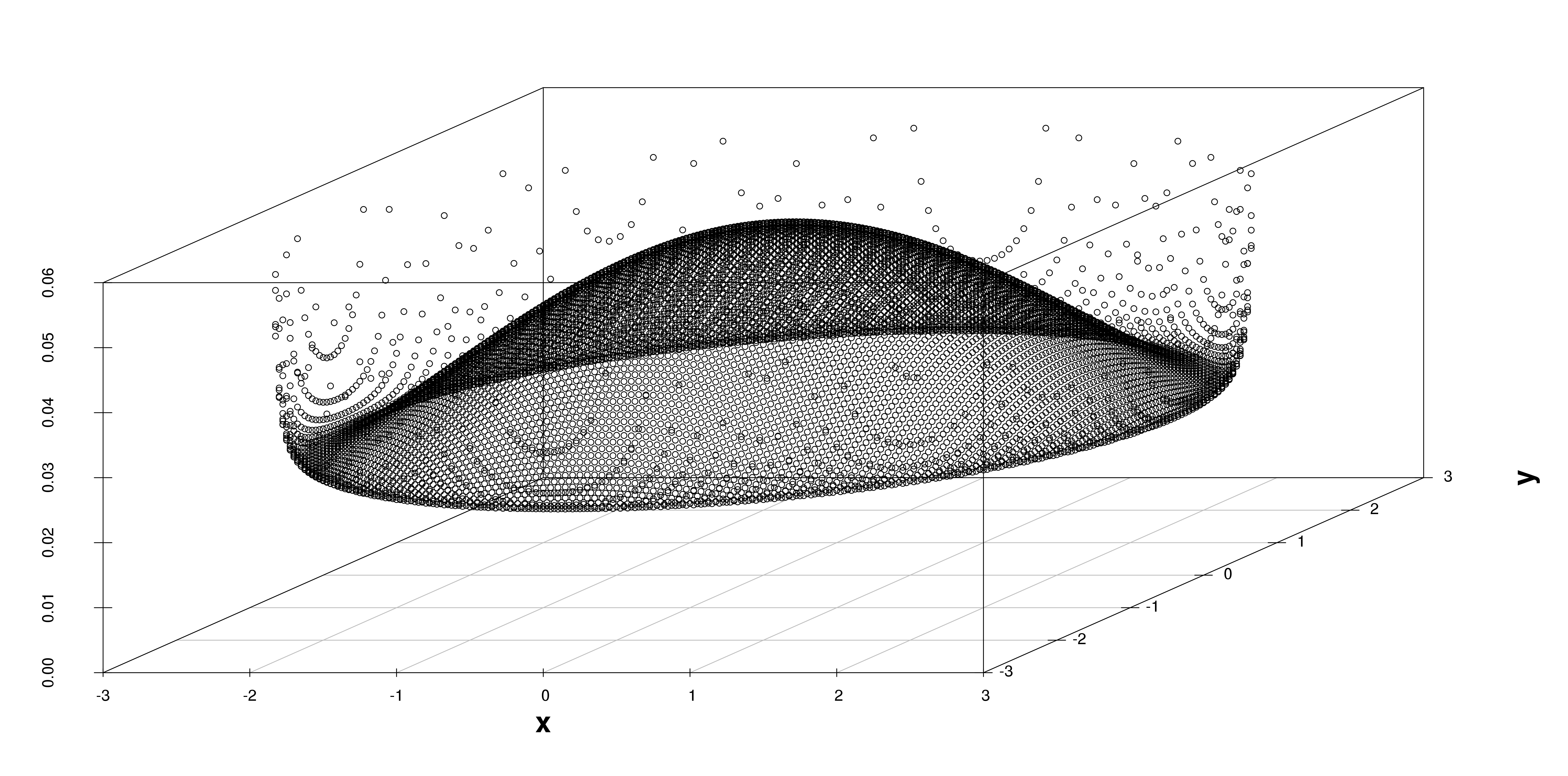
Figure 2. Behavior of the distribution (5.12) for $\lambda=c=1$ and $t=3$.

We observe that in this case, the planar motion develops completely inside the circle $C_{ct}$. Moreover a remarkable relation can be found with the process studied in [7]. We also recall that in [7] the governing equation of this planar motion was given and it corresponds to the following telegraph equation with time-dependent coefficient

(5.13) $$\left(\frac{\partial^{2}}{\partial t^{2}}+2\lambda\coth(\lambda t)\frac{\partial}{\partial t}-c^{2}\Delta\right)p(x,y,t)=0.$$

We now consider the complementary case where the particle changes direction only at even-order Poisson times. In this case we have the following

Theorem 5.5.

The distribution of the planar random motion $(X(t),Y(t))$, when the changes of direction are taken only at even-order Poisson times is given by

(5.14) $$P\{X(t)\in dx,Y(t)\in dy\}=\frac{\lambda}{2\pi c}\frac{1}{\cosh(\lambda t)}\frac{\sinh\left(\frac{\lambda}{c}\sqrt{c^{2}t^{2}-(x^{2}+y^{2})}\right)}{\sqrt{c^{2}t^{2}-(x^{2}+y^{2})}}dxdy,$$

where $(x,y)\in intC_{ct}$.

Proof.

In view of Theorem 5.3 we have

$$P\{X(t)\in dx,Y(t)\in dy\}$$

$$=\sum_{n=0}^{\infty}P\{X(t)\in dx,Y(t)\in dy|N(t)=2n\}P\{N(t)=2n|\bigcup_{k=0}^{\infty}\{N(t)=2k\}\}$$

$$=\sum_{n=0}^{\infty}\frac{(2n)}{2\pi(ct)^{2n}}\left[\sqrt{c^{2}t^{2}-(x^{2}+y^{2})}\right]^{2n-2}\frac{2(\lambda t)^{2n}e^{-\lambda t}}{(1+e^{-2\lambda t})(2n)!}dxdy$$

$$=\frac{\lambda}{2\pi c}\frac{1}{\cosh(\lambda t)}\sum_{n=0}^{\infty}\left(\frac{\lambda}{c}\right)^{2n+1}\frac{\left[\sqrt{c^{2}t^{2}-(x^{2}+y^{2})}\right]^{2n+1}}{(2n+1)!}dxdy$$

$$=\frac{\lambda}{2\pi c}\frac{1}{\cosh(\lambda t)}\frac{\sinh\left(\frac{\lambda}{c}\sqrt{c^{2}t^{2}-(x^{2}+y^{2})}\right)}{\sqrt{c^{2}t^{2}-(x^{2}+y^{2})}}dxdy,$$

as claimed. ∎

In this case the singular component of the distribution is concentrated on $\partial C_{ct}$ and is given by

(5.15) $$\int_{-ct}^{+ct}P\{X(t)\in dx,Y(t)\in dy\}=1-\frac{1}{\cosh(\lambda t)},$$

where

(5.16) $$\frac{1}{\cosh(\lambda t)}=P\{N(t)=0|\bigcup_{k=0}^{\infty}\{N(t)=2k\}\}.$$

The density (5.14) has a bell–shaped form (see Figure 3) with a singular part of weight (5.16) on $\partial C_{ct}$.

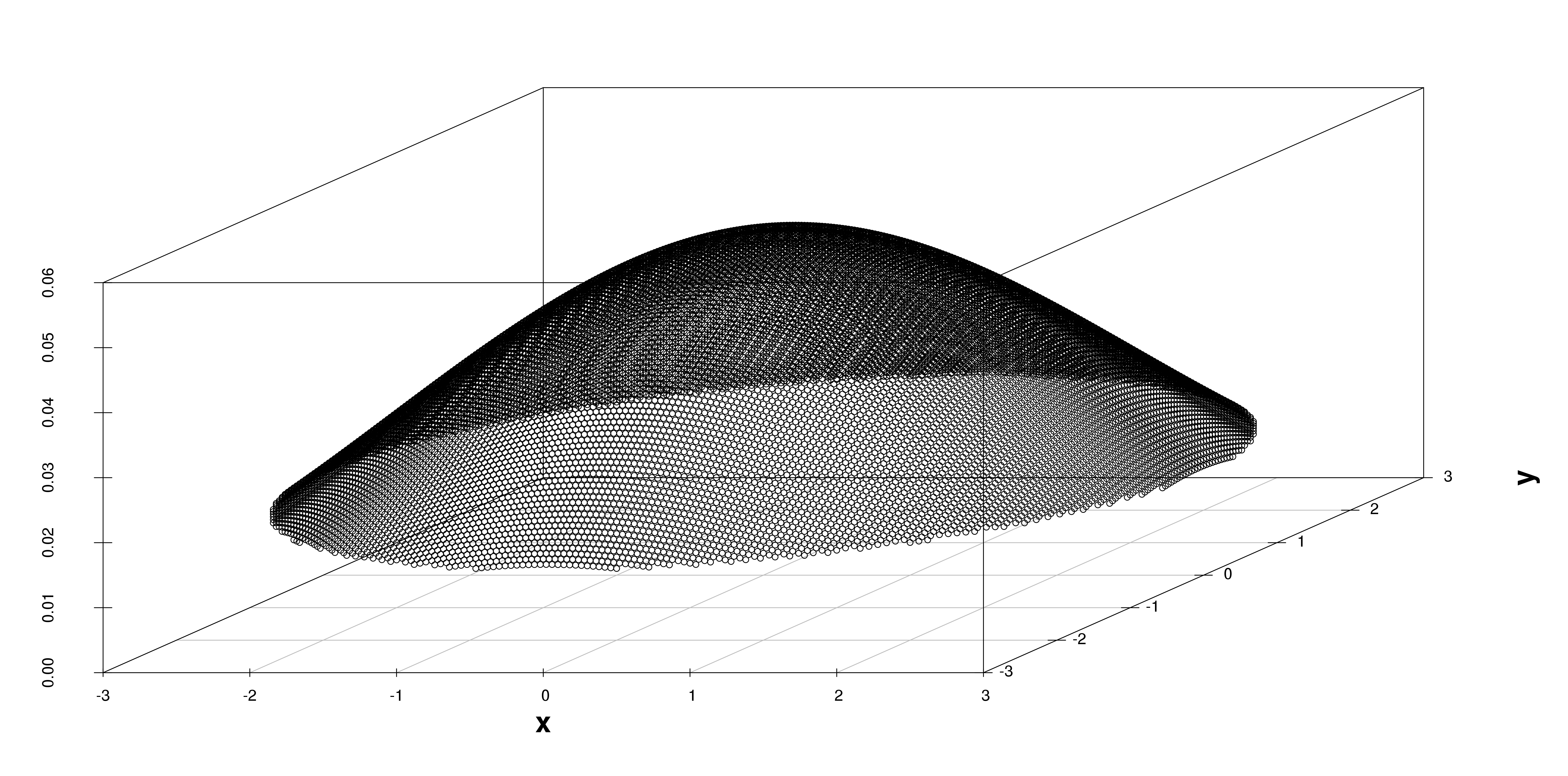
Figure 3. Behavior of the distribution (5.14) for $\lambda=c=1$ and $t=3$.

It is simple to prove the following

Proposition 5.6.

The density law of the planar random motion with density (5.14) is governed by the following telegraph-type equation

(5.17) $$\left(\frac{\partial^{2}}{\partial t^{2}}+2\lambda\tanh(\lambda t)\frac{\partial}{\partial t}-c^{2}\Delta\right)p(x,y,t)=0.$$

Acknowledgement. The authors gratefully acknowledge the appreciation of their work by the referee as well as his/her suggestions and comments.

References

- [1] I.F. Barna and R. Kersner, Heat conduction: a telegraph-type model with self-similar behavior of solutions, J. Phys. A, 43, 375210, (2010)
- [2] D.W. Bresters, On the equation of Euler-Poisson-Darboux, SIAM Journal of Mathematical Analysis, 4: 31–41, (1973)
- [3] A. De Gregorio, E. Orsingher, L.Sakhno, Motions with finite velocity analyzed with order statistics and differential equations, Probability Theory and Mathematical Statistics, 71, 57-71, (2004)
- [4] A. De Gregorio, E. Orsingher, Flying randomly in with Dirichlet displacements, Stochastic processes and their applications, 122:676–713, (2012)
- [5] A. Erdélyi, On the Euler-Poisson-Darboux equation, Journal d’Analyse Mathématique, 23(1), 89–102, (1970)
- [6] S.K. Foong, U. van Kolck, Poisson Random Walk for Solving Wave Equations, Progress of Theoretical Physics, 87(2): 285–292, (1992)
- [7] R. Garra, E. Orsingher, Random flights governd by Klein–Gordon-type partial differential equations, Stochastic Processes and their Applications, 124, 2171–2187, (2014)
- [8] R. Garra, E. Orsingher, F. Polito, Fractional Klein–-Gordon Equations and Related Stochastic Processes, Journal of Statistical Physics, 155(4), 777–809, (2014)
- [9] S.M. Iacus, Statistical analysis of the inhomogeneous telegrapher’s process, Statistics and Probability Letters, 55: 83–88, (2001)
- [10] S. Kaplan, Differential equations in which the Poisson process plays a role, Bull. Amer. Math. Soc., 70(2):264–268, (1964)
- [11] A.D. Kolesnik, E .Orsingher. A planar random motion with an infinite number of directions controlled by the damped wave equation, Journal of Applied Probability, 42(4):1168–1182, (2005)
- [12] G. Le Caër, A Pearson–-Dirichlet random walk, J. Stat. Phys.: 140 (2010) 728–751.
- [13] G. Le Caër, A new family of solvable Pearson–-Dirichlet random walks, J. Stat. Phys.: 144 (2011) 23–45.
- [14] A.C. McBride. Fractional Powers of a Class of Ordinary Differential Operators, Proceedings of the London Mathematical Society, 3(45):519–546, (1982)
- [15] M.N. Olevskii, An Operator Approach to the Cauchy Problem for the Euler–Poisson–Darboux Equation in Spaces of Constant Curvature, Integral Equations and Operator Theory, 49(1):77–109, (2004)
- [16] E .Orsingher, A.D. Kolesnik. Exact distribution for a planar random motion model, controlled by a fourth-order hyperbolic equation, Theory of Probability and its Applications, 41(2),451-459, (1996)
- [17] E. Orsingher, Exact joint distribution in a model of planar random motion, Stochastics and Stochastics Reports, 69:1–10, (2000)
- [18] S.I. Rosencrans, Diffusion Transforms, Journal of Differential Equations, 13, 457–467, (1973)
- [19] S. Samko, A. Kilbas, O. Marichev : Fractional Integrals and Derivatives, Gordon and Breach Science Publishers, Minsk, Belarus (1987)
- [20] W. Stadje. The exact probability distribution of a two-dimensional random walk, Journal of Statistical Physics, 46(1–2):207–216, (1987)
- [21] W. Stadje, S. Zacks, Telegraph processes with random velocities, J. Appl. Probab. 41 (3) (2004) 665–678.