extremal1

QMUL-PH-14-23

Centre for Research in String Theory
School of Physics and Astronomy
Queen Mary, University of London
Mile End Road, London E1 4NS, United Kingdom

d.young@qmul.ac.uk

An Extremal Chiral Primary Three-Point Function at Two-loops in ABJ(M)

Donovan Young

1 Introduction and result

This paper is a continuation of the works [1, 2, 3], where it has been pointed out that the ${\cal N}=6$ Chern-Simons matter theory of Aharony, Bergman, Jafferis, and Maldacena (ABJM) [4, 5] presents a nice lab for looking at three-point functions because, unlike ${\cal N}=4$ SYM, the protected chiral primary operators don’t have protected three-point functions. These operators are defined by

$${\cal O}^{J}_{A}=\frac{1}{\sqrt{J/2}}\left(\frac{k}{4\pi\sqrt{NM}}\right)^{J/2}({\cal C}_{A})^{A_{1}\ldots A_{J/2}}_{B_{1}\ldots B_{J/2}}\,\mathop{\mathrm{Tr}}\left(Y^{B_{1}}Y^{\dagger}_{A_{1}}\cdots Y^{B_{J/2}}Y^{\dagger}_{A_{J/2}}\right),$$ (1)

where the $Y^{A_{i}=1,2,3,4}$ are the bifundamental $(N,\bar{M})$ complex scalars of the theory, $k$ is the Chern-Simons level and ${\cal C}_{A}$ is a traceless symmetric tensor. Their conformally-fixed three-point functions

$$\bigl{\langle}{\cal O}_{1}(x_{1}){\cal O}_{2}(x_{2}){\cal O}_{3}(x_{3})\bigr{\rangle}=\frac{1}{(4\pi)^{\gamma}}\frac{C_{123}(\lambda,\hat{\lambda})}{|x_{12}|^{\gamma_{3}}|x_{23}|^{\gamma_{1}}|x_{31}|^{\gamma_{2}}},$$ (2)

where $\gamma_{i}=(\sum_{j}J_{j}-2J_{i})/2$, $\gamma=\gamma_{1}+\gamma_{2}+\gamma_{3}$, and $x_{ij}=x_{i}-x_{j}$, include non-trivial dependence of the structure constant $C_{123}$ on the ’t Hooft couplings $\lambda=N/k$, $\hat{\lambda}=M/k$. At strong coupling, and in the ABJM case where $N=M$, supergravity tells us that [6, 1]

$$\begin{split}&C_{123}(\lambda\gg 1)=\\ &\frac{1}{N}\left(\frac{\lambda}{2\pi^{2}}\right)^{1/4}\frac{\prod_{i=1}^{3}\sqrt{J_{i}+1}\,(J_{i}/2)!\,\Gamma(\gamma_{i}/2+1)}{\Gamma(\gamma/2+1)}\\ &\sum_{p=0}^{\gamma_{3}}\frac{\left({\cal C}_{1}\right)^{I_{1}\ldots I_{p}I_{p+1}\ldots I_{J_{1}/2}}_{K_{1}\ldots K_{\gamma_{3}-p}K_{\gamma_{3}-p+1}\ldots K_{J_{1}/2}}\left({\cal C}_{2}\right)^{K_{1}\ldots K_{\gamma_{3}-p}L_{1}\ldots L_{\gamma_{1}-J_{2}/2+p}}_{I_{1}\ldots I_{p}M_{1}\ldots M_{J_{2}/2-p}}\left({\cal C}_{3}\right)^{K_{\gamma_{3}-p+1}\ldots K_{J_{1}/2}M_{1}\ldots M_{J_{2}/2-p}}_{I_{p+1}\ldots I_{J_{1}/2}L_{1}\ldots L_{\gamma_{1}-J_{2}/2+p}}}{p!(\gamma_{3}-p)!(\gamma_{1}-J_{2}/2+p)!(J_{2}/2-p)!(\gamma_{2}-J_{1}/2+p)!(J_{1}/2-p)!},\end{split}$$ (3)

and suggests a series of interpolating functions corresponding to the independent ways the ${\cal C}$-tensors can be contracted.

The case of extremal correlators – when $J_{3}=J_{1}+J_{2}$ – offers a dramatic simplification. In this case we have a single possible contraction (labelled “tree” for reasons to be explained directly) and obtain

$$C_{123}^{\text{extremal}}(\lambda\gg 1)=\frac{1}{N}\left(\frac{\lambda}{2\pi^{2}}\right)^{1/4}\sqrt{(J_{1}+1)(J_{2}+1)(J_{3}+1)}\,\langle{\cal C}_{1}{\cal C}_{2}{\cal C}_{3}\rangle_{\text{tree}}.$$ (4)

This expression is similar to the tree-level expression

$$C_{123}(\lambda\to 0)=C_{F}\sqrt{(J_{1}/2)(J_{2}/2)(J_{3}/2)}\,\langle{\cal C}_{1}\,{\cal C}_{2}\,{\cal C}_{3}\rangle_{\text{tree}},$$ (5)

and thus suggests a simplification compared to the non-extremal case. In this paper I compute the structure constant at leading loop order for the simplest such extremal correlator consisting of one length-four operator and two length-two operators. The result is

$$C_{123}\bigl{|}_{{\cal O}(\lambda^{2})}=\frac{\pi^{2}}{6}\left(\lambda^{2}+\hat{\lambda}^{2}\right).$$ (6)

For the ABJM case where $N=M$ the strong coupling result is (4)

$$C_{123}(\lambda\to\infty)=\left(\frac{\lambda}{2\pi^{2}}\right)^{1/4}\frac{3\sqrt{5}}{2\sqrt{2}},$$ (7)

and thus $C_{123}$ interpolates between $1+\lambda^{2}\pi^{2}/3$ and this value. It remains a very interesting direction of future research to determine this interpolating function exactly.

In the following sections of the paper I review the method of calculation first presented in [3], and give an account of the various Feynman diagrams contributing to the result. The appendices contain the details of the reduction to master integrals and the presentation of the master integrals themselves. We have used the dimensional regularization scheme adopted in [7, 8] where $d=2\omega=3-2\epsilon$ and all numerators are reduced to scalar products at the physical dimension first, while loop integration proceeds as usual using dimensional regularization. The conventions used here are identical to those used in very similar contexts in [8, 2, 3] and the reader is directed to these works for statements of the action, Feynman rules and other details.

2 Spacetime point integration method

In [3] a novel method for computing three-point functions of protected operators was suggested. The idea is to exploit the finiteness of the three-point function by integrating over one of the spacetime points where one of the three operators is sitting, using the same dimensional regularization scheme used in the loop computation. This reduces the required Feynman integrals to propagator-type, which are more easily evaluated.

In the case of two length-two and one length-four operator in ABJM, this integration is itself convergent if we choose the point where the length-four operator sits to integrate over. We will look at the following specific operators

$$\begin{split}&{\cal O}_{1}=\frac{k}{4\pi\sqrt{MN}}\mathop{\mathrm{Tr}}(Y^{1}Y^{\dagger}_{2}),\\ &{\cal O}_{2}=\frac{k^{2}}{\sqrt{2}(4\pi)^{2}MN}\Bigl{(}\mathop{\mathrm{Tr}}(Y^{2}Y^{\dagger}_{1}Y^{4}Y^{\dagger}_{3})+\mathop{\mathrm{Tr}}(Y^{\dagger}_{1}Y^{2}Y^{\dagger}_{3}Y^{4})\Bigr{)},\\ &{\cal O}_{3}=\frac{k}{4\pi\sqrt{MN}}\mathop{\mathrm{Tr}}(Y^{3}Y^{\dagger}_{4}).\end{split}$$ (8)

The three-point function is

$$\bigl{\langle}{\cal O}_{1}(0){\cal O}_{2}(x){\cal O}_{3}(y)\bigr{\rangle}=\frac{1}{\sqrt{2}}\left(\frac{1}{N}+\frac{1}{M}\right)\frac{1}{(4\pi)^{4}}\frac{\hat{C}_{123}(\lambda,\hat{\lambda})}{x^{2}(x-y)^{2}}.$$ (9)

Integrating over $x$, we obtain

$$\int d^{3}x\bigl{\langle}{\cal O}_{1}(0){\cal O}_{2}(x){\cal O}_{3}(y)\bigr{\rangle}=\frac{1}{\sqrt{2}}\left(\frac{1}{N}+\frac{1}{M}\right)\frac{\hat{C}_{123}(\lambda,\hat{\lambda})}{256\pi|y|},$$ (10)

and so

$$\hat{C}_{123}(\lambda,\hat{\lambda})=256\pi|y|\sqrt{2}\left(\frac{1}{N}+\frac{1}{M}\right)^{-1}\int d^{3}x\bigl{\langle}{\cal O}_{1}(0){\cal O}_{2}(x){\cal O}_{3}(y)\bigr{\rangle}.$$ (11)

Thus the task is to calculate $\int d^{3}x\bigl{\langle}{\cal O}_{1}(0){\cal O}_{2}(x){\cal O}_{3}(y)\bigr{\rangle}$, which in momentum space amounts to setting to zero the momentum flowing into the central operator. We thus obtain four-loop propagator-type diagrams which we tackle in the following section.

The structure constant is renormalized by the two-point functions of the three operators according to

$$C_{123}\bigl{|}_{{\cal O}(\lambda^{2})}=\left[\hat{C}_{123}-\frac{1}{2}\sum_{i=1}^{3}g_{i}\right]_{{\cal O}(\lambda^{2})}.$$ (12)

where

$$\begin{split}&\bigl{\langle}{\cal O}_{1}(x){\cal O}_{1}(0)\bigr{\rangle}=\frac{g_{1}(\lambda,\hat{\lambda})}{(4\pi|x|)^{2}},\quad\bigl{\langle}{\cal O}_{2}(x){\cal O}_{2}(0)\bigr{\rangle}=\frac{g_{2}(\lambda,\hat{\lambda})}{(4\pi|x|)^{4}},\\ &\bigl{\langle}{\cal O}_{3}(x){\cal O}_{3}(0)\bigr{\rangle}=\frac{g_{3}(\lambda,\hat{\lambda})}{(4\pi|x|)^{2}},\end{split}$$ (13)

and where $g_{i}(0,0)=1$.

3 Feynman diagrammatics

We will require the two-loop decorations of the (integrated) tree-level correlator

(70,70) v1 v2 plain,right=1v1,va,v2,va,v1 decor.shape=circle,decor.filled=30,decor.size=9v1 decor.shape=circle,decor.filled=30,decor.size=9v2

where we have indicated the length-two operators with grey blobs. The first thing to notice is that diagrams in which only one of the two loops are decorated

(90,90) v1 v2 plain,right=0.8v1,va,vb,v2,vb,va,v1 decor.shape=circle,decor.filled=30,decor.size=9v1 decor.shape=circle,decor.filled=30,decor.size=9v2 d.sh=circle,l.d=0, d.f=10,d.si=.3w,l=$2$va

are removed by the $g_{1}$ and $g_{3}$ terms of the renormalization (12). We thus move on to the diagrams in which decorations connect the right and left loops. Many potential diagrams evaluate to zero via two mechanisms. The first is that a gauge field line drawn across two legs of an operator (from one scalar-scalar-gauge vertex on each leg) will produce zero as long as it can be contracted to the operator site (i.e. without encountering other vertices along the way) [2]. Examples of these types of diagrams are

$$\parbox{56.9055pt}{\vspace{1.5cm} \fmfgraph*(40,70) \fmftop{v1} \fmfleft{v2} \fmfright{v3} \fmfv{decoration.shape=circle,decoration.filled=30,decor.size=9}{v1} \fmf{plain}{v1,vc1} \fmf{plain}{vc1,vc3} \fmf{plain}{vc3,v2} \fmf{plain}{v1,vc2} \fmf{plain}{vc2,vc4} \fmf{plain}{vc4,v3} \fmffreeze\fmf{photon,right=0.15}{vc1,vc2} \fmffreeze\fmfposition}=\hskip 14.22636pt\parbox{56.9055pt}{\vspace{1.5cm} \fmfgraph*(40,70) \fmftop{v1} \fmfleft{v2} \fmfright{v3} \fmfv{decoration.shape=circle,decoration.filled=30,decor.size=9}{v1} \fmf{plain}{v1,vc1} \fmf{plain}{vc1,vc3} \fmf{plain}{vc3,v2} \fmf{plain}{v1,vc2} \fmf{plain}{vc2,vc4} \fmf{plain}{vc4,v3} \fmffreeze\fmf{photon,right=0.15}{vc1,vc2} \fmf{photon,right=0.15}{vc3,vc4} \fmffreeze\fmfposition}=\hskip 14.22636pt\parbox{56.9055pt}{\vspace{.4cm} \fmfgraph*(40,40) \fmftop{v1} \fmfstraight\fmfbottom{v2,v3,v4} \fmfv{decoration.shape=circle,decoration.filled=30,decor.size=9}{v1} \fmf{plain}{v1,vc1} \fmf{plain}{vc1,v2} \fmf{plain}{v1,vc2} \fmf{plain}{vc2,vcc2} \fmf{plain}{vcc2,v3} \fmf{plain}{v1,vc3} \fmf{plain}{vc3,v4} \fmffreeze\fmf{photon}{vc1,vc2} \fmf{photon}{vcc2,vc3} }=~{}~{}0.$$

The second mechanism is encountered when a single gauge field connects to the left or right loop

$$\parbox{56.9055pt}{ \fmfgraph*(70,70) \fmfleft{v1} \fmfright{v2} \fmfbottom{b1} \fmf{plain,right=0.2}{v1,va} \fmf{plain,right=0.2}{va,v2} \fmf{plain,right=0.3}{v2,v1} \fmf{wiggly}{b1,va} \fmfv{decor.shape=circle,decor.filled=30,decor.size=9}{v2} }~{}\qquad+~{}~{}~{}\parbox{56.9055pt}{ \fmfgraph*(70,70) \fmfleft{v1} \fmfright{v2} \fmftop{t1} \fmf{plain,left=0.2}{v1,va} \fmf{plain,left=0.2}{va,v2} \fmf{plain,left=0.3}{v2,v1} \fmf{wiggly}{t1,va} \fmfv{decor.shape=circle,decor.filled=30,decor.size=9}{v2} }~{}\qquad=~{}0,$$

here the sum of connecting the lone gauge field to the top line of the loop and to the bottom produces zero via a simple integration by parts. Note that in the above we have not shown the left loop where the gauge field originates. We are then left with a series of non-vanishing diagrams, which have been collected in table 1.

(50,50) v1 v5 t2,t4,t3 b1 plain,left=0.5, tension=0.75v1,v2 plain,left=0.4, tension=1v2,v3 plain,left=0.4, tension=1v3,v4 plain,left=0.5, tension=0.75v4,v5 plain,left=1., tension=1v5,v3,v1 phantom,tension=2.8t2,v2 phantom,tension=2.8t3,v4 phantom,tension=1.05v3,b1 wiggly,left=.3v2,v4 wiggly,left=.9v2,v4 decor.shape=circle,decor.filled=30,decor.size=9v1 decor.shape=circle,decor.filled=30,decor.size=9v5	(50,50) v1 v5 t2,t4,t3 b2,b1,b3 plain,left=0.35, tension=0.75v1,vb plain,left=0.2, tension=114.25vb,v2 plain,left=0.4, tension=1v2,v3 plain,left=1., tension=1v3,v5 plain,left=0.35, tension=.75v5,vc plain,left=0.2, tension=114.25vc,v4 plain,left=0.4, tension=1v4,v3 plain,left=1., tension=1v3,v1 phantom,tension=3.t4,v2 phantom,tension=6t2,vb phantom,tension=3.b1,v4 phantom,tension=6b3,vc wiggly,right=2.3,tension=1vc,v2 wiggly,left=2.3,tension=1v4,vb decor.shape=circle,decor.filled=30,decor.size=9v1 decor.shape=circle,decor.filled=30,decor.size=9v5	(50,50) v1 v5 t2,t4,t3 b1 plain,left=0.35, tension=0.75v1,vb plain,left=0.1, tension=0.25vb,v2 plain,left=0.4, tension=1v2,v3 plain,left=0.4, tension=1v3,v4 plain,left=0.5, tension=0.75v4,v5 plain,left=1., tension=1v5,v3,v1 phantom,tension=2.8t2,v2 phantom,tension=1.t2,vb phantom,tension=2.8t3,v4 phantom,tension=1.05v3,b1 wiggly,left=.3v2,v4 wiggly,left=.7,tension=0.1vb,v4 decor.shape=circle,decor.filled=30,decor.size=9v1 decor.shape=circle,decor.filled=30,decor.size=9v5	(50,50) v1 v5 t2,t4,t3 b2,b1,b3 plain,left=0.35, tension=0.75v1,vb plain,left=0.2, tension=114.25vb,v2 plain,left=0.4, tension=1v2,v3 plain,left=1., tension=1v3,v5 plain,left=0.35, tension=.75v5,vc plain,left=0.2, tension=4.25vc,v4 plain,left=0.3, tension=1v4,v3 plain,left=1., tension=1v3,v1 phantom,tension=3.t4,v2 phantom,tension=6t2,vb phantom,tension=3.b1,v4 phantom,tension=6b3,vc wiggly,right=1.93,tension=1vc,v2 wiggly,left=1.93,tension=1v4,vb decor.shape=circle,decor.filled=30,decor.size=9v1 decor.shape=circle,decor.filled=30,decor.size=9v5	(50,50) v1 v5 t2,t4,t3 b2,b1,b3 plain,left=0.5, tension=0.75v1,v2 plain,left=0.25, tension=2v2,v3 plain,left=0.4, tension=1v3,v4 plain,left=0.4, tension=0.75v4,v5 plain,left=1.1, tension=1v5,v3 plain,left=0.6, tension=0.75v3,v6 plain,left=0.4, tension=1v6,v1 phantom,tension=2.2t2,v2 phantom,tension=4.2t3,v4 phantom,tension=.35v3,b1 phantom,tension=6.8v6,b2 wiggly,left=.8v2,v4 wiggly,left=2.05v6,v4 decor.shape=circle,decor.filled=30,decor.size=9v1 decor.shape=circle,decor.filled=30,decor.size=9v5
(50,50) v1 v5 t2,t4,t3 b2,b1,b3 plain,left=0.35, tension=0.75v1,vb plain,left=0.2, tension=4.25vb,v2 plain,left=0.3, tension=1v2,v3 plain,left=1., tension=1v3,v5 plain,left=0.35, tension=.75v5,vc plain,left=0.2, tension=4.25vc,v4 plain,left=0.3, tension=1v4,v3 plain,left=1., tension=1v3,v1 phantom,tension=3.t4,v2 phantom,tension=6t2,vb phantom,tension=3.b1,v4 phantom,tension=6b3,vc wiggly,right=1.93,tension=1vc,v2 wiggly,left=1.93,tension=1v4,vb decor.shape=circle,decor.filled=30,decor.size=9v1 decor.shape=circle,decor.filled=30,decor.size=9v5	(50,50) v1 v5 t2,t4,t3 b2,b1,b3 plain,left=0.35, tension=0.75v1,vb plain,left=0.2, tension=114.25vb,v2 plain,left=0.4, tension=1v2,v3 plain,left=1., tension=1v3,v5 plain,left=0.35, tension=.75v5,vc plain,left=0.2, tension=114.25vc,v4 plain,left=0.4, tension=1v4,v3 plain,left=1., tension=1v3,v1 phantom,tension=3.t4,v2 phantom,tension=6t2,vb phantom,tension=3.b1,v4 phantom,tension=6b3,vc dashes,right=2.3,tension=1vc,v2 dashes,left=2.3,tension=1v4,vb decor.shape=circle,decor.filled=30,decor.size=9v1 decor.shape=circle,decor.filled=30,decor.size=9v5	(50,50) v1 v3 plain,left=0.3, tension=1v1,v4,v3,v2,v1 (0,33)v2,v4 plain,left=.93v2,v5 dashes,left=.93v5,v4 plain,right=.93v2,v5 dashes,right=.93v5,v4 decor.shape=circle,decor.filled=30,decor.size=9v1 decor.shape=circle,decor.filled=30,decor.size=9v3	(50,50) v1 v3 t1,t2 b1,b2 plain,left=.8, tension=1v1,v4,v5,v3,v4,v1 plainv4,v5 plain,right=.93v4,v5 phantom,tension=1t1,v4 phantom,tension=4t2,v5 decor.shape=circle,decor.filled=30,decor.size=9v1 decor.shape=circle,decor.filled=30,decor.size=9v3

Table 1: Decorations of the three-point correlator. Unique diagrams obtained through reflection about the horizontal and vertical axes must also be considered.

(50,50) v1 v3 plain,left=0.3, tension=1v1,v4,v3,v2,v1 plain,left=1., tension=1v1,v3,v1 (0,33)v2,v4 wiggly,left=.3v2,v4,v2 decor.shape=circle,decor.filled=30,decor.size=9v1 decor.shape=circle,decor.filled=30,decor.size=9v3	(50,50) v1 t v2 b1,b2 phantom,tension=2.95t,va phantom,tension=2.15b1,vb1 phantom,tension=2.15b2,vb2 plain,left=0.3v1,va plain,left=0.3va,v2 plain,right=0.25v1,vb1 plain,right=0.25vb1,vb2 plain,right=0.25vb2,v2 wigglyva,vb1 wigglyva,vb2 plain,left=1., tension=1v1,v2 plain,left=1.2, tension=1v2,v1 decor.shape=circle,decor.filled=30,decor.size=9v1 decor.shape=circle,decor.filled=30,decor.size=9v2	(50,50) v1 t1,t2,t3 v2 b phantom,tension=1.0t1,va1 phantom,tension=1.1t2,va2 phantom,tension=1.0t3,va3 phantom,tension=2.95b,vb plain,left=0.17v1,va1 plain,left=0.15va1,va2 plain,left=0.15va2,va3 plain,left=0.17va3,v2 plain,right=0.3v1,vb plain,right=0.3vb,v2 wiggly,left=0.75va1,va3 wigglyva2,vb plain,left=1.3, tension=1v1,v2 plain,left=1., tension=1v2,v1 decor.shape=circle,decor.filled=30,decor.size=9v1 decor.shape=circle,decor.filled=30,decor.size=9v2	(50,50) v1 t1,t2,t3 v2 b phantom,tension=1.0t1,va1 phantom,tension=1.1t2,va2 phantom,tension=1.0t3,va3 phantom,tension=2.95b,vb plain,left=0.17v1,va1 plain,left=0.15va1,va2 plain,left=0.15va2,va3 plain,left=0.17va3,v2 plain,right=0.3v1,vb plain,right=0.3vb,v2 wigglyva1,vcen wigglyva3,vcen wigglyvb,vcen plain,left=1.2, tension=1v1,v2 plain,left=1., tension=1v2,v1 decor.shape=circle,decor.filled=30,decor.size=9v1 decor.shape=circle,decor.filled=30,decor.size=9v2	(50,50) v1 v3 plain,left=0.3, tension=1v1,v4,v3,v2,v1 (0,33)v2,v4 wigglyv2,vc,v4 plain,left=1., tension=1v1,v3,v1 d.sh=circle,l.d=0, d.f=empty,d.si=.25w,l=$1$vc decor.shape=circle,decor.filled=30,decor.size=9v1 decor.shape=circle,decor.filled=30,decor.size=9v3
(50,50) v1 v3 plain,left=1., tension=1v1,va dashes,left=1., tension=1va,vb plain,left=1., tension=1vb,v3 plain,right=1., tension=1v1,va dashes,right=1., tension=1va,vb plain,right=1., tension=1vb,v3 plain,left=.75, tension=1v1,v3,v1 decor.shape=circle,decor.filled=30,decor.size=9v1 decor.shape=circle,decor.filled=30,decor.size=9v3	(50,50) v1 v3 plain,left=0.3, tension=1v1,v4,v3,v2,v1 (0,30)v2,v4 plain,left=1., tension=1v1,v3,v1 d.sh=circle,l.d=0, d.f=empty,d.si=.25w,l=$2$v4 decor.shape=circle,decor.filled=30,decor.size=9v1 decor.shape=circle,decor.filled=30,decor.size=9v3	(50,50) v1 v3 plain,left=0.93, tension=1v1,v4 plain, tension=1v1,v4 plain,right=0.93, tension=1v1,v4 plain,left=0.93, tension=1v4,v3 plain, tension=1v4,v3 plain,right=0.93, tension=1v4,v3 plain,left=1., tension=1v3,v1 decor.shape=circle,decor.filled=30,decor.size=9v1 decor.shape=circle,decor.filled=30,decor.size=9v3	(50,50) v1 v3 t1 b1 plain,left=0.3, tension=1v1,v4,v3 plain, tension=1v1,v2,v3 plain,right=.3, tension=1v1,v5,v3 plain,right=1, tension=1v1,v3 phantom,tension=5b1,v5 phantom,tension=5t1,v4 wigglyv2,v5 wigglyv2,v4 decor.shape=circle,decor.filled=30,decor.size=9v1 decor.shape=circle,decor.filled=30,decor.size=9v3

Table 2: The Feynman diagrams which contribute to the two-point function of the length-four operator. The various decorations must be considered on all sets of adjacent legs. Unique diagrams obtained through reflection about the vertical axis must also be considered.

These diagrams are evaluated using the Feynman rules published in [8] (note that these Feynman rules capture only the planar contributions which is sufficient for the present calculation) and used already in [2, 3]. The resulting integrals are then reduced to master integrals using the LiteRed package of Roman N. Lee [9], and in particular the “p4.zip” basis provided on his website. One then requires the $\epsilon$-expansion of these master integrals generically out to ${\cal O}(\epsilon^{2})$. In four-dimensions these integrals have been evaluated to high-orders in the $\epsilon$-expansion [10], starting with the original work [11] which used the glue-and-cut symmetry, and using the method of dimensional-recurrence and analyticity also pioneered by Lee [12]. The author is very grateful to Prof. Lee for providing the three-dimensional epsilon expansion of the required integrals out to 500-digit accuracy which have allowed this computation to be executed [13].

We must also evaluate the finite renormalization of the two-point function for the length-four operator. The diagrams required are shown in table 2. They are mostly captured by the three-loop propagator diagrams encountered in [3] but the final two diagrams require the same four-loop integrals discussed above.

We conclude this section with a statement of the results. The reduction of the individual diagrams to master integrals is given in appendix B, and in appendix A we quote the results for the master integrals in an $\epsilon$-expansion about three-dimensions. In table 1 the following diagrams add to zero at ${\cal O}(\epsilon^{0})$

$$\parbox{56.9055pt}{ \fmfgraph*(50,50) \fmfleft{v1} \fmfright{v5} \fmftop{t2,t4,t3} \fmfbottom{b1} \fmf{plain,left=0.5, tension=0.75}{v1,v2} \fmf{plain,left=0.4, tension=1}{v2,v3} \fmf{plain,left=0.4, tension=1}{v3,v4} \fmf{plain,left=0.5, tension=0.75}{v4,v5} \fmf{plain,left=1., tension=1}{v5,v3,v1} \fmf{phantom,tension=2.8}{t2,v2} \fmf{phantom,tension=2.8}{t3,v4} \fmf{phantom,tension=1.05}{v3,b1} \fmf{wiggly,left=.3}{v2,v4} \fmf{wiggly,left=.9}{v2,v4} \fmfv{decor.shape=circle,decor.filled=30,decor.size=9}{v1} \fmfv{decor.shape=circle,decor.filled=30,decor.size=9}{v5} }+\hskip 17.07182pt\parbox{56.9055pt}{ \fmfgraph*(50,50) \fmfleft{v1} \fmfright{v5} \fmftop{t2,t4,t3} \fmfbottom{b2,b1,b3} \fmf{plain,left=0.35, tension=0.75}{v1,vb} \fmf{plain,left=0.2, tension=114.25}{vb,v2} \fmf{plain,left=0.4, tension=1}{v2,v3} \fmf{plain,left=1., tension=1}{v3,v5} \fmf{plain,left=0.35, tension=.75}{v5,vc} \fmf{plain,left=0.2, tension=114.25}{vc,v4} \fmf{plain,left=0.4, tension=1}{v4,v3} \fmf{plain,left=1., tension=1}{v3,v1} \fmf{phantom,tension=3.}{t4,v2} \fmf{phantom,tension=6}{t2,vb} \fmf{phantom,tension=3.}{b1,v4} \fmf{phantom,tension=6}{b3,vc} \fmf{wiggly,right=2.3,tension=1}{vc,v2} \fmf{wiggly,left=2.3,tension=1}{v4,vb} \fmfv{decor.shape=circle,decor.filled=30,decor.size=9}{v1} \fmfv{decor.shape=circle,decor.filled=30,decor.size=9}{v5} }~{}~{}~{}~{}+\hskip 17.07182pt\parbox{56.9055pt}{ \fmfgraph*(50,50) \fmfleft{v1} \fmfright{v5} \fmftop{t2,t4,t3} \fmfbottom{b2,b1,b3} \fmf{plain,left=0.35, tension=0.75}{v1,vb} \fmf{plain,left=0.2, tension=114.25}{vb,v2} \fmf{plain,left=0.4, tension=1}{v2,v3} \fmf{plain,left=1., tension=1}{v3,v5} \fmf{plain,left=0.35, tension=.75}{v5,vc} \fmf{plain,left=0.2, tension=114.25}{vc,v4} \fmf{plain,left=0.4, tension=1}{v4,v3} \fmf{plain,left=1., tension=1}{v3,v1} \fmf{phantom,tension=3.}{t4,v2} \fmf{phantom,tension=6}{t2,vb} \fmf{phantom,tension=3.}{b1,v4} \fmf{phantom,tension=6}{b3,vc} \fmf{dashes,right=2.3,tension=1}{vc,v2} \fmf{dashes,left=2.3,tension=1}{v4,vb} \fmfv{decor.shape=circle,decor.filled=30,decor.size=9}{v1} \fmfv{decor.shape=circle,decor.filled=30,decor.size=9}{v5} }~{}~{}~{}~{}+\hskip 8.5359pt\parbox{56.9055pt}{ \fmfgraph*(50,50) \fmfleft{v1} \fmfright{v3} \fmftop{t1,t2} \fmfbottom{b1,b2} \fmf{plain,left=.8, tension=1}{v1,v4,v5,v3,v4,v1} \fmf{plain}{v4,v5} \fmf{plain,right=.93}{v4,v5} \fmf{phantom,tension=1}{t1,v4} \fmf{phantom,tension=4}{t2,v5} \fmfv{decor.shape=circle,decor.filled=30,decor.size=9}{v1} \fmfv{decor.shape=circle,decor.filled=30,decor.size=9}{v3} }={\cal O}(\epsilon).$$

The remaining diagrams are individually finite and sum to

$$\text{sum of diagrams in Table \ref{tab:maindiags}}\stackrel{{\scriptstyle 500}}{{\approx}}-\frac{1}{\sqrt{2}}\frac{(M+N)}{k^{2}}\frac{\pi^{2}}{192(p^{2})^{7-4\omega}},$$ (14)

where the result has been verified to 500 digits of accuracy. Using (11) we find

$$\hat{C}_{123}(\lambda,\hat{\lambda})=1-\lambda\hat{\lambda}\frac{\pi^{2}}{3}+{\cal O}(\lambda^{2}).$$ (15)

The two-point function evaluates to

$$\text{sum of diagrams in Table \ref{tab:twoptdiags}}\stackrel{{\scriptstyle 500}}{{\approx}}(\lambda+\hat{\lambda})^{2}\frac{1}{768(p^{2})^{7-5\omega}},$$ (16)

and using (LABEL:twoptnorm) we find

$$g_{2}(\lambda,\hat{\lambda})=1-\frac{\pi^{2}}{3}(\lambda+\hat{\lambda})^{2}.$$ (17)

Finally using (12) we obtain (6).

Appendix A Master integrals

The master integrals required for the calculation are a subset of the basis presented in [11]; they have been collected in figure 1. The integrals $M_{21}$, $M_{22}$, $M_{34}$, $M_{35}$, $M_{36}$, $M_{44}$, $M_{45}$, $M_{51}$ cannot be reduced to $G$-functions or $F$-functions. Their values have been computed using the dimensional recurrence analyticity method of Lee [12] and their values out to 500 digits have been shared with me [13]. The algorithm PSLQ [14] has been used in certain places to provide analytical results for terms in the $\epsilon$-expansion.

We use $d^{2\omega}l/(2\pi)^{2\omega}$ as the loop integration measure where $d=2\omega=3-2\epsilon$. The $G$ and $F$ functions are given by

$$G(\alpha,\beta)=\frac{1}{(4\pi)^{\omega}}\frac{\Gamma(\alpha+\beta-\omega)\,\Gamma(\omega-\alpha)\,\Gamma(\omega-\beta)}{\Gamma(\alpha)\,\Gamma(\beta)\,\Gamma(2\omega-\alpha-\beta)},$$ (18)

and [15, 16]

$$\begin{split}&F_{\lambda}=\frac{2}{(4\pi)^{2\omega}}\,\Gamma(\omega-1)\,\Gamma(\omega-\lambda-1)\,\Gamma(\lambda-2\omega+3)\Biggl{(}-\frac{\pi\cot\left(\pi(2\omega-\lambda)\right)}{\Gamma(2\omega-2)}\\ &+\frac{\Gamma(\omega-1)\,{}_{3}F_{2}\left(1,2+\lambda-\omega,2\omega-2;\lambda+1,\lambda-\omega+3;1\right)}{(\omega-\lambda-2)\,\Gamma(1+\lambda)\,\Gamma(3\omega-\lambda-4)}\,\Biggr{)}.\end{split}$$ (19)

The Fourier transform is defined as

$$\int\frac{d^{2\omega}p}{(2\pi)^{2\omega}}\frac{e^{ip\cdot x}}{[p^{2}]^{s}}=\frac{\Gamma(\omega-s)}{4^{s}\pi^{\omega}\Gamma(s)}\frac{1}{[x^{2}]^{\omega-s}}.$$ (20)

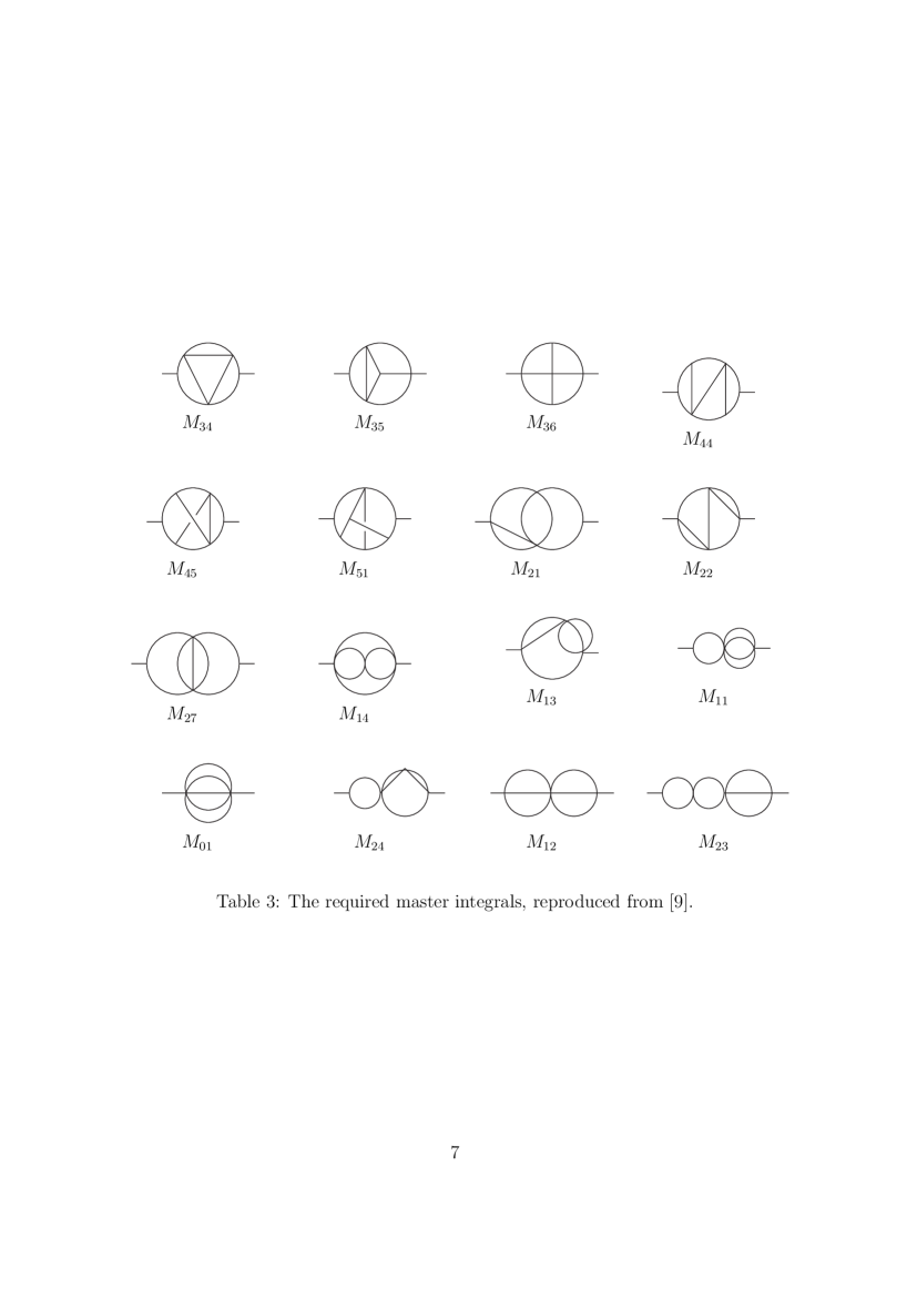
Figure 1: The four-loop master integrals required for the three-point function, reproduced from [11].

Below we employ a convenient normalization for the presentation of the $\epsilon$-expansion of the integrals

$${\cal M}=(4\pi)^{2-4\omega}e^{-4\gamma\epsilon}.$$ (21)

$$\begin{split}&M_{34}={\cal M}\left(-\frac{\pi^{2}}{32\epsilon}+\frac{\pi^{2}}{16}\left(3-2\log 2\right)+\left(\frac{37\pi^{4}}{96}-\frac{\pi^{2}}{8}\bigl{(}2\log 2(\log 2-3)+9\bigr{)}\right)\epsilon+{\cal O}(\epsilon^{2})\right),\\ &M_{35}={\cal M}\Bigl{(}\frac{1}{16\epsilon^{2}}+\frac{1}{16}(3\pi^{2}-60)-10.1695380240468262091170104661503731482787\epsilon\\ &+5.761640224581950185485181492971261298252179\epsilon^{2}+{\cal O}(\epsilon^{3})\Bigr{)},\\ &M_{36}={\cal M}\Bigl{(}\frac{1}{8\epsilon^{2}}+\frac{1}{4\epsilon}+\frac{\pi^{2}}{24}-4-31.24683122358910241344375025381651547680\epsilon\\ &-104.97997949576156077918973047903786740\epsilon^{2}+{\cal O}(\epsilon^{3})\Bigr{)},\\ &M_{44}={\cal M}\Bigl{(}\frac{1}{8\epsilon^{2}}+\frac{1}{4\epsilon}+\frac{5\pi^{2}}{24}-4-8.154600887744206655212139477314414443076\epsilon\\ &+65.5962689793108431307288614828060453748\epsilon^{2}+{\cal O}(\epsilon^{3})\Bigr{)},\\ &M_{45}={\cal M}\Bigl{(}\frac{1}{8\epsilon^{2}}+\frac{25\pi^{2}}{24}-\frac{31}{2}-25.73103829909166269503717808059699905229\epsilon\\ &+52.4026571263842398765902744496356247875\epsilon^{2}+{\cal O}(\epsilon^{3})\Bigr{)},\\ &M_{51}={\cal M}\Bigl{(}\frac{1}{8\epsilon^{2}}+\left(\frac{263}{120}-\frac{4\pi^{2}}{45}\right)\frac{1}{\epsilon}+1.3455583077571687466389820840805296520163\\ &-54.1517695706215470260568776499507551760225\epsilon+{\cal O}(\epsilon^{2})\Bigr{)},\\ &M_{21}={\cal M}\bigl{(}5.462481216887406375320255581095582681248891250+{\cal O}(\epsilon)\bigr{)},\\ &M_{22}={\cal M}\bigl{(}5.462481216887406375320255581095582681248891250+{\cal O}(\epsilon)\bigr{)}.\\ \end{split}$$ (22)

$$\begin{split}&M_{27}=F_{3-2\omega},\quad M_{14}=G(1,1)^{2}\,G(1,4-2\omega)\,G(1,5-3\omega),\\ &M_{13}=G(1,1)^{2}\,G(1,2-\omega)\,G(1,5-3\omega),\quad M_{11}=G(1,1)^{2}\,G(1,2-\omega)\,G(1,3-2\omega),\\ &M_{01}=G(1,1)\,G(1,2-\omega)\,G(1,3-2\omega)\,G(1,4-3\omega),\\ &M_{24}=G(1,1)^{3}\,G(1,4-2\omega),\quad M_{12}=G^{2}(1,1)\,G^{2}(1,2-\omega),\\ &M_{23}=G(1,1)^{3}\,G(1,2-\omega).\end{split}$$ (23)

Appendix B Reduction to master integrals

B.1 Three-point function diagrams

I give below the reduction of the integrated three-point function in terms of basis integrals. This reduction was performed using the code LiteRed [9]. An overall factor of $(4\pi/k)^{2}$ is suppressed. The colour factors of the diagrams are all equal to $(M+N)/\sqrt{2}$.

$$\parbox{56.9055pt}{ \fmfgraph*(50,50) \fmfleft{v1} \fmfright{v5} \fmftop{t2,t4,t3} \fmfbottom{b1} \fmf{plain,left=0.5, tension=0.75}{v1,v2} \fmf{plain,left=0.4, tension=1}{v2,v3} \fmf{plain,left=0.4, tension=1}{v3,v4} \fmf{plain,left=0.5, tension=0.75}{v4,v5} \fmf{plain,left=1., tension=1}{v5,v3,v1} \fmf{phantom,tension=2.8}{t2,v2} \fmf{phantom,tension=2.8}{t3,v4} \fmf{phantom,tension=1.05}{v3,b1} \fmf{wiggly,left=.3}{v2,v4} \fmf{wiggly,left=.9}{v2,v4} \fmfv{decor.shape=circle,decor.filled=30,decor.size=9}{v1} \fmfv{decor.shape=circle,decor.filled=30,decor.size=9}{v5} }=\hskip 17.07182pt\parbox{56.9055pt}{ \fmfgraph*(50,50) \fmfleft{v1} \fmfright{v5} \fmftop{t2,t4,t3} \fmfbottom{b2,b1,b3} \fmf{plain,left=0.35, tension=0.75}{v1,vb} \fmf{plain,left=0.2, tension=114.25}{vb,v2} \fmf{plain,left=0.4, tension=1}{v2,v3} \fmf{plain,left=1., tension=1}{v3,v5} \fmf{plain,left=0.35, tension=.75}{v5,vc} \fmf{plain,left=0.2, tension=114.25}{vc,v4} \fmf{plain,left=0.4, tension=1}{v4,v3} \fmf{plain,left=1., tension=1}{v3,v1} \fmf{phantom,tension=3.}{t4,v2} \fmf{phantom,tension=6}{t2,vb} \fmf{phantom,tension=3.}{b1,v4} \fmf{phantom,tension=6}{b3,vc} \fmf{wiggly,right=2.3,tension=1}{vc,v2} \fmf{wiggly,left=2.3,tension=1}{v4,vb} \fmfv{decor.shape=circle,decor.filled=30,decor.size=9}{v1} \fmfv{decor.shape=circle,decor.filled=30,decor.size=9}{v5} }~{}~{}~{}~{}=-4\hskip 17.07182pt\parbox{56.9055pt}{ \fmfgraph*(50,50) \fmfleft{v1} \fmfright{v5} \fmftop{t2,t4,t3} \fmfbottom{b2,b1,b3} \fmf{plain,left=0.35, tension=0.75}{v1,vb} \fmf{plain,left=0.2, tension=114.25}{vb,v2} \fmf{plain,left=0.4, tension=1}{v2,v3} \fmf{plain,left=1., tension=1}{v3,v5} \fmf{plain,left=0.35, tension=.75}{v5,vc} \fmf{plain,left=0.2, tension=114.25}{vc,v4} \fmf{plain,left=0.4, tension=1}{v4,v3} \fmf{plain,left=1., tension=1}{v3,v1} \fmf{phantom,tension=3.}{t4,v2} \fmf{phantom,tension=6}{t2,vb} \fmf{phantom,tension=3.}{b1,v4} \fmf{phantom,tension=6}{b3,vc} \fmf{dashes,right=2.3,tension=1}{vc,v2} \fmf{dashes,left=2.3,tension=1}{v4,vb} \fmfv{decor.shape=circle,decor.filled=30,decor.size=9}{v1} \fmfv{decor.shape=circle,decor.filled=30,decor.size=9}{v5} }~{}~{}~{}=M_{11}\left(\frac{1}{2\omega-3}+2\right)$$

$$+M_{14}\left(\frac{5}{12(3\omega-4)}-\frac{25}{12}\right)+M_{34}\left(\frac{1}{4}-\frac{1}{4(3\omega-4)}\right),$$

$$\parbox{56.9055pt}{ \fmfgraph*(50,50) \fmfleft{v1} \fmfright{v5} \fmftop{t2,t4,t3} \fmfbottom{b1} \fmf{plain,left=0.35, tension=0.75}{v1,vb} \fmf{plain,left=0.1, tension=0.25}{vb,v2} \fmf{plain,left=0.4, tension=1}{v2,v3} \fmf{plain,left=0.4, tension=1}{v3,v4} \fmf{plain,left=0.5, tension=0.75}{v4,v5} \fmf{plain,left=1., tension=1}{v5,v3,v1} \fmf{phantom,tension=2.8}{t2,v2} \fmf{phantom,tension=1.}{t2,vb} \fmf{phantom,tension=2.8}{t3,v4} \fmf{phantom,tension=1.05}{v3,b1} \fmf{wiggly,left=.3}{v2,v4} \fmf{wiggly,left=.7,tension=0.1}{vb,v4} \fmfv{decor.shape=circle,decor.filled=30,decor.size=9}{v1} \fmfv{decor.shape=circle,decor.filled=30,decor.size=9}{v5} }=\hskip 14.22636pt\parbox{56.9055pt}{ \fmfgraph*(50,50) \fmfleft{v1} \fmfright{v5} \fmftop{t2,t4,t3} \fmfbottom{b2,b1,b3} \fmf{plain,left=0.35, tension=0.75}{v1,vb} \fmf{plain,left=0.2, tension=114.25}{vb,v2} \fmf{plain,left=0.4, tension=1}{v2,v3} \fmf{plain,left=1., tension=1}{v3,v5} \fmf{plain,left=0.35, tension=.75}{v5,vc} \fmf{plain,left=0.2, tension=4.25}{vc,v4} \fmf{plain,left=0.3, tension=1}{v4,v3} \fmf{plain,left=1., tension=1}{v3,v1} \fmf{phantom,tension=3.}{t4,v2} \fmf{phantom,tension=6}{t2,vb} \fmf{phantom,tension=3.}{b1,v4} \fmf{phantom,tension=6}{b3,vc} \fmf{wiggly,right=1.93,tension=1}{vc,v2} \fmf{wiggly,left=1.93,tension=1}{v4,vb} \fmfv{decor.shape=circle,decor.filled=30,decor.size=9}{v1} \fmfv{decor.shape=circle,decor.filled=30,decor.size=9}{v5} }~{}~{}~{}=M_{11}\left(-\frac{1}{4(2\omega-3)^{2}}-\frac{15}{4(2\omega-3)}-\frac{13}{2}\right)$$

$$+M_{14}\left(-\frac{5}{4(3\omega-4)}+\frac{1}{2(2\omega-3)}+\frac{35}{4}\right)+M_{34}\left(\frac{3}{4(3\omega-4)}-\frac{3}{4}\right)+M_{27},$$

$$\parbox{56.9055pt}{ \fmfgraph*(50,50) \fmfleft{v1} \fmfright{v5} \fmftop{t2,t4,t3} \fmfbottom{b2,b1,b3} \fmf{plain,left=0.5, tension=0.75}{v1,v2} \fmf{plain,left=0.25, tension=2}{v2,v3} \fmf{plain,left=0.4, tension=1}{v3,v4} \fmf{plain,left=0.4, tension=0.75}{v4,v5} \fmf{plain,left=1.1, tension=1}{v5,v3} \fmf{plain,left=0.6, tension=0.75}{v3,v6} \fmf{plain,left=0.4, tension=1}{v6,v1} \fmf{phantom,tension=2.2}{t2,v2} \fmf{phantom,tension=4.2}{t3,v4} \fmf{phantom,tension=.35}{v3,b1} \fmf{phantom,tension=6.8}{v6,b2} \fmf{wiggly,left=.8}{v2,v4} \fmf{wiggly,left=2.05}{v6,v4} \fmfv{decor.shape=circle,decor.filled=30,decor.size=9}{v1} \fmfv{decor.shape=circle,decor.filled=30,decor.size=9}{v5} }=M_{01}\left(\frac{2}{(2\omega-3)^{2}}-\frac{6752}{27(3\omega-5)}-\frac{2240}{27(3\omega-5)^{2}}+\frac{560}{3(5\omega-8)}-\frac{2}{3(2\omega-3)}-\frac{1340}{27}\right)$$

$$+M_{11}\left(\frac{13}{6(2\omega-3)^{2}}+\frac{20}{3\omega-5}+\frac{112}{15(5\omega-8)}+\frac{7}{2(2\omega-3)}+\frac{93}{5}\right)$$

$$+M_{13}\left(-\frac{1}{3(2\omega-3)^{2}}-\frac{16}{3(3\omega-5)}-\frac{16}{3(5\omega-8)}-\frac{4}{3(2\omega-3)}-\frac{31}{3}\right)$$

$$+M_{14}\left(-\frac{100}{27(3\omega-5)}-\frac{16}{27(3\omega-5)^{2}}-\frac{1}{2\omega-3}-\frac{235}{27}\right)$$

$$+2M_{22}\left(-\frac{8}{15(5\omega-8)}-\frac{8}{9(3\omega-5)}+\frac{52}{45}\right)+M_{27}\left(-\frac{4}{3(3\omega-5)}-\frac{4}{3(2\omega-3)}-\frac{10}{3}\right)$$

$$+M_{35}\left(\frac{1}{3(2\omega-3)^{2}}+\frac{4}{15(5\omega-8)}-\frac{4}{3(2\omega-3)}+\frac{13}{15}\right)+M_{45}\left(-\frac{1}{12(2\omega-3)^{2}}+\frac{1}{6(2\omega-3)}-\frac{1}{12}\right),$$

$$\parbox{56.9055pt}{ \fmfgraph*(50,50) \fmfleft{v1} \fmfright{v5} \fmftop{t2,t4,t3} \fmfbottom{b2,b1,b3} \fmf{plain,left=0.35, tension=0.75}{v1,vb} \fmf{plain,left=0.2, tension=4.25}{vb,v2} \fmf{plain,left=0.3, tension=1}{v2,v3} \fmf{plain,left=1., tension=1}{v3,v5} \fmf{plain,left=0.35, tension=.75}{v5,vc} \fmf{plain,left=0.2, tension=4.25}{vc,v4} \fmf{plain,left=0.3, tension=1}{v4,v3} \fmf{plain,left=1., tension=1}{v3,v1} \fmf{phantom,tension=3.}{t4,v2} \fmf{phantom,tension=6}{t2,vb} \fmf{phantom,tension=3.}{b1,v4} \fmf{phantom,tension=6}{b3,vc} \fmf{wiggly,right=1.93,tension=1}{vc,v2} \fmf{wiggly,left=1.93,tension=1}{v4,vb} \fmfv{decor.shape=circle,decor.filled=30,decor.size=9}{v1} \fmfv{decor.shape=circle,decor.filled=30,decor.size=9}{v5} }~{}~{}~{}=M_{01}\Bigl{(}\frac{19691}{16(\omega-2)^{2}}+\frac{1575}{8(\omega-2)^{3}}+\frac{45}{2(\omega-2)^{4}}+\frac{2333}{32(2\omega-3)}-\frac{17}{(2\omega-3)^{2}}$$

$$-\frac{3}{(2\omega-3)^{3}}+\frac{280}{3(3\omega-5)}+\frac{55531}{16(4\omega-7)}+\frac{1617}{4(4\omega-7)^{2}}-\frac{560}{5\omega-8}+\frac{10711}{16(\omega-2)}+\frac{65185}{96}\Bigr{)}$$

$$+M_{11}\left(\frac{29}{(\omega-2)^{2}}+\frac{6}{(\omega-2)^{3}}+\frac{2}{2\omega-3}-\frac{2}{(2\omega-3)^{2}}-\frac{10}{4\omega-7}-\frac{112}{5(5\omega-8)}+\frac{52}{\omega-2}+\frac{131}{5}\right)$$

$$M_{12}\Bigl{(}\frac{14}{(\omega-2)^{2}}+\frac{7}{2(\omega-2)^{3}}-\frac{1}{2(2\omega-3)}-\frac{1}{8(2\omega-3)^{2}}-\frac{1155}{64(4\omega-7)}-\frac{175}{128(4\omega-7)^{2}}$$

$$-\frac{8}{5(5\omega-8)}+\frac{231}{8(\omega-2)}+\frac{7497}{640}\Bigr{)}+M_{13}\Bigl{(}-\frac{163}{4(\omega-2)^{2}}-\frac{33}{4(\omega-2)^{3}}+\frac{4}{2\omega-3}+\frac{3}{4(2\omega-3)^{2}}$$

$$+\frac{3285}{128(4\omega-7)}+\frac{525}{256(4\omega-7)^{2}}+\frac{16}{5\omega-8}-\frac{1323}{16(\omega-2)}-\frac{7239}{256}\Bigr{)}$$

$$+M_{14}\left(\frac{8}{3(3\omega-5)}+\frac{10}{3(3\omega-4)}+\frac{115}{4(4\omega-7)}+\frac{105}{16(4\omega-7)^{2}}-\frac{15}{\omega-2}-\frac{1015}{48}\right)$$

$$+2M_{22}\left(-\frac{2}{(\omega-2)^{2}}-\frac{2}{4\omega-7}+\frac{8}{5(5\omega-8)}-\frac{6}{\omega-2}-\frac{34}{5}\right)$$

$$+M_{27}\left(-\frac{7}{(\omega-2)^{2}}+\frac{3}{2\omega-3}-\frac{35}{4(4\omega-7)}-\frac{35}{2(\omega-2)}-\frac{43}{4}\right)$$

$$+M_{34}\left(\frac{1}{2(2\omega-3)}-\frac{2}{3\omega-4}+\frac{5}{16(4\omega-7)}-\frac{5}{4(\omega-2)}-\frac{37}{16}\right)$$

$$+M_{35}\left(\frac{1}{2(2\omega-3)^{2}}+\frac{3}{16(4\omega-7)}-\frac{4}{5(5\omega-8)}-\frac{7}{8(2\omega-3)}+\frac{87}{80}\right)$$

$$+M_{36}\left(-\frac{1}{8(2\omega-3)^{2}}-\frac{5}{128(4\omega-7)}+\frac{13}{512(4\omega-7)^{2}}+\frac{2}{5(5\omega-8)}-\frac{23}{128(2\omega-3)}+\frac{303}{2560}\right)$$

$$+M_{51}\left(-\frac{3}{128(4\omega-7)}-\frac{21}{512(4\omega-7)^{2}}+\frac{15}{128(2\omega-3)}-\frac{27}{512}\right),$$

$$\parbox{56.9055pt}{ \fmfgraph*(50,50) \fmfleft{v1} \fmfright{v3} \fmf{plain,left=0.3, tension=1}{v1,v4,v3,v2,v1} \fmffixed{(0,33)}{v2,v4} \fmf{plain,left=.93}{v2,v5} \fmf{dashes,left=.93}{v5,v4} \fmf{plain,right=.93}{v2,v5} \fmf{dashes,right=.93}{v5,v4} \fmfv{decor.shape=circle,decor.filled=30,decor.size=9}{v1} \fmfv{decor.shape=circle,decor.filled=30,decor.size=9}{v3} }=-2\,G(1,1)\,F_{3-2\omega},$$

$$\parbox{56.9055pt}{ \fmfgraph*(50,50) \fmfleft{v1} \fmfright{v3} \fmftop{t1,t2} \fmfbottom{b1,b2} \fmf{plain,left=.8, tension=1}{v1,v4,v5,v3,v4,v1} \fmf{plain}{v4,v5} \fmf{plain,right=.93}{v4,v5} \fmf{phantom,tension=1}{t1,v4} \fmf{phantom,tension=4}{t2,v5} \fmfv{decor.shape=circle,decor.filled=30,decor.size=9}{v1} \fmfv{decor.shape=circle,decor.filled=30,decor.size=9}{v3} }=G^{2}(1,1)\,G(1,2-\omega)\,G(1,4-2\omega).$$

B.2 Two-point function diagrams

The two-point function of the length-four operator is essential for renormalizing the three-point function. Here I give the reduction to master integrals which was performed in a very similar context in [3]. Again, a factor of $(4\pi/k)^{2}$ is suppressed while the colour factors for the various diagrams are

$$T_{1},T_{2},T_{4},T_{6}=2(M^{2}+N^{2}),\qquad T_{3},T_{5},T_{8},T_{9}=4MN.$$ (24)

The scalar propagator at two loops involves the quantity [8]

$$\begin{split}Z_{\text{scalar}}&=-\frac{1}{(4\pi)^{2}}\Biggl{[}MN\left(\frac{3}{4(3-2\omega)}+\frac{1}{4}\left(-\frac{3\pi^{2}}{2}+25-3\gamma+3\log(4\pi)\right)\right)\\ &+\frac{(M-N)^{2}}{4}\left(\frac{1}{2(3-2\omega)}-\frac{\pi^{2}}{4}+\frac{1}{2}\left(3-\gamma+\log(4\pi)\right)\right)\Biggr{]}+{\cal O}(\epsilon).\end{split}$$ (25)

The following three-loop master integrals are employed here

$$P_{1}=\parbox{56.9055pt}{ \fmfgraph*(70,70) \fmfleft{i} \fmfright{o} \fmf{plain,tension=4}{i,v1} \fmf{plain,tension=4}{v3,o} \fmf{plain,left=1}{v1,va,v3,va,v1} \fmffreeze\fmf{plain}{v1,va} }\quad=G^{2}(1,1)\,G(1,2-\omega),\quad P_{2}=\parbox{56.9055pt}{ \fmfgraph*(50,50) \fmfleft{i} \fmfright{o} \fmf{plain,tension=4}{i,v1} \fmf{plain,tension=4}{v3,o} \fmf{plain,left=1}{v1,va,v3,va,v1} \fmffreeze\fmf{plain,left=1.}{v1,v3} }=G^{2}(1,1)\,G(1,4-2\omega),$$

$$P_{3}=\parbox{56.9055pt}{ \fmfgraph*(60,60) \fmfleft{i} \fmfright{o} \fmftop{t} \fmfbottom{b} \fmf{phantom,tension=1.7}{t,va} \fmf{phantom,tension=1.7}{b,vb} \fmf{plain,tension=4}{i,v1} \fmf{plain,tension=4}{v3,o} \fmf{plain,left=0.3}{v1,va,v3,vb,v1} \fmffreeze\fmf{plain,right=0.5}{va,vb,va} }\,=G(1,1)\,F_{2-\omega},~{}P_{4}=\parbox{56.9055pt}{ \fmfgraph*(60,60) \fmfleft{i} \fmfright{o} \fmf{plain,tension=8}{i,v1} \fmf{plain,tension=8}{v3,o} \fmf{plain,left=1}{v1,v3,v1} \fmf{plain,left=0.5}{v1,v3,v1} }\,=G(1,1)\,G(1,2-\omega)\,G(1,3-2\omega),$$

$$P_{6}=\parbox{56.9055pt}{ \fmfgraph*(60,60) \fmfleft{i} \fmfright{o} \fmf{plain,tension=4}{i,v1} \fmf{plain,tension=4}{v3,o} \fmf{plain,left=1}{v1,v3} \fmf{plain,tension=2}{v1,va} \fmf{plain}{va,vb} \fmf{plain,tension=2}{vb,v3} \fmffreeze\fmf{plain,left=1.}{va,vb,va} }\,=G(1,1)\,G(1,2-\omega)\,G(1,5-2\omega),\hskip 8.5359ptP_{7}=\parbox{56.9055pt}{ \fmfgraph*(50,50) \fmfleft{i} \fmfright{o} \fmf{plain,tension=4}{i,v1} \fmf{plain,tension=4}{v3,o} \fmf{plain,tension=3}{v1,vc} \fmf{plain,tension=3}{vd,v3} \fmf{plain,left=1}{vc,va,vd,va,vc} \fmffreeze\fmf{plain,left=.9}{v1,v3} }\,=G^{2}(1,1)\,G(1,6-2\omega).$$

The reductions are as follows

$$T_{1}=~{}~{}\parbox{56.9055pt}{ \fmfgraph*(50,50) \fmfleft{v1} \fmfright{v3} \fmf{plain,left=0.3, tension=1}{v1,v4,v3,v2,v1} \fmf{plain,left=1., tension=1}{v1,v3,v1} \fmffixed{(0,33)}{v2,v4} \fmf{wiggly,left=.3}{v2,v4,v2} \fmfv{decor.shape=circle,decor.filled=30,decor.size=9}{v1} \fmfv{decor.shape=circle,decor.filled=30,decor.size=9}{v3} }=G(1,5-3\omega)\,G(1,6-4\omega)\left(\frac{P_{3}(3-2\omega)}{4(3\omega-4)}+\frac{1}{6}P_{4}\left(\frac{1}{3\omega-4}+\frac{3}{2\omega-3}+10\right)\right),$$

$$T_{2}=~{}~{}\parbox{56.9055pt}{ \fmfgraph*(50,50) \fmfleft{v1} \fmftop{t} \fmfright{v2} \fmfbottom{b1,b2} \fmf{phantom,tension=2.95}{t,va} \fmf{phantom,tension=2.15}{b1,vb1} \fmf{phantom,tension=2.15}{b2,vb2} \fmf{plain,left=0.3}{v1,va} \fmf{plain,left=0.3}{va,v2} \fmf{plain,right=0.25}{v1,vb1} \fmf{plain,right=0.25}{vb1,vb2} \fmf{plain,right=0.25}{vb2,v2} \fmffreeze\fmf{wiggly}{va,vb1} \fmf{wiggly}{va,vb2} \fmf{plain,left=1., tension=1}{v1,v2} \fmf{plain,left=1.2, tension=1}{v2,v1} \fmfv{decor.shape=circle,decor.filled=30,decor.size=9}{v1} \fmfv{decor.shape=circle,decor.filled=30,decor.size=9}{v2} }=G(1,5-3\omega)\,G(1,6-4\omega)\Biggl{(}\frac{P_{3}(9-6\omega)}{16-12\omega}+P_{4}\left(\frac{1}{8-6\omega}+\frac{1}{3-2\omega}-4\right)$$

$$+P_{1}-\frac{P_{2}}{2}\Biggr{)},$$

$$T_{3}=~{}~{}~{}\parbox{56.9055pt}{ \fmfgraph*(50,50) \fmfleft{v1} \fmftop{t1,t2,t3} \fmfright{v2} \fmfbottom{b} \fmf{phantom,tension=1.0}{t1,va1} \fmf{phantom,tension=1.1}{t2,va2} \fmf{phantom,tension=1.0}{t3,va3} \fmf{phantom,tension=2.95}{b,vb} \fmf{plain,left=0.17}{v1,va1} \fmf{plain,left=0.15}{va1,va2} \fmf{plain,left=0.15}{va2,va3} \fmf{plain,left=0.17}{va3,v2} \fmf{plain,right=0.3}{v1,vb} \fmf{plain,right=0.3}{vb,v2} \fmffreeze\fmf{wiggly,left=0.75}{va1,va3} \fmf{wiggly}{va2,vb} \fmf{plain,left=1.3, tension=1}{v1,v2} \fmf{plain,left=1., tension=1}{v2,v1} \fmfv{decor.shape=circle,decor.filled=30,decor.size=9}{v1} \fmfv{decor.shape=circle,decor.filled=30,decor.size=9}{v2} }=2T_{4}=\hskip 11.38092pt\parbox{56.9055pt}{ \fmfgraph*(50,50) \fmfleft{v1} \fmftop{t1,t2,t3} \fmfright{v2} \fmfbottom{b} \fmf{phantom,tension=1.0}{t1,va1} \fmf{phantom,tension=1.1}{t2,va2} \fmf{phantom,tension=1.0}{t3,va3} \fmf{phantom,tension=2.95}{b,vb} \fmf{plain,left=0.17}{v1,va1} \fmf{plain,left=0.15}{va1,va2} \fmf{plain,left=0.15}{va2,va3} \fmf{plain,left=0.17}{va3,v2} \fmf{plain,right=0.3}{v1,vb} \fmf{plain,right=0.3}{vb,v2} \fmffreeze\fmf{wiggly}{va1,vcen} \fmf{wiggly}{va3,vcen} \fmf{wiggly}{vb,vcen} \fmf{plain,left=1.2, tension=1}{v1,v2} \fmf{plain,left=1., tension=1}{v2,v1} \fmfv{decor.shape=circle,decor.filled=30,decor.size=9}{v1} \fmfv{decor.shape=circle,decor.filled=30,decor.size=9}{v2} }=G(1,5-3\omega)\,G(1,6-4\omega)\Biggl{(}P_{1}\left(\frac{2}{2\omega-3}+4\right)$$

$$+\frac{P_{3}(5-4\omega)}{4-3\omega}-\frac{2P_{4}(\omega-1)(4\omega-5)(8\omega-11)}{(3-2\omega)^{2}(3\omega-4)}-4P_{2},\Biggr{)}$$

$$T_{5}=~{}~{}~{}\parbox{56.9055pt}{ \fmfgraph*(50,50) \fmfleft{v1} \fmfright{v3} \fmf{plain,left=0.3, tension=1}{v1,v4,v3,v2,v1} \fmffixed{(0,33)}{v2,v4} \fmf{wiggly}{v2,vc,v4} \fmf{plain,left=1., tension=1}{v1,v3,v1} \fmfv{d.sh=circle,l.d=0, d.f=empty,d.si=.25w,l=$1$}{vc} \fmfv{decor.shape=circle,decor.filled=30,decor.size=9}{v1} \fmfv{decor.shape=circle,decor.filled=30,decor.size=9}{v3} }=G(1,5-3\omega)\,G(1,6-4\omega)\Biggl{(}\frac{P_{3}(5-4\omega)}{3\omega-4}+P_{4}\left(\frac{2}{12-9\omega}+\frac{12}{\omega-2}+\frac{40}{3}\right)\Biggr{)},$$

$$T_{6}=~{}~{}~{}\parbox{56.9055pt}{ \fmfgraph*(50,50) \fmfleft{v1} \fmfright{v3} \fmf{plain,left=1., tension=1}{v1,va} \fmf{dashes,left=1., tension=1}{va,vb} \fmf{plain,left=1., tension=1}{vb,v3} \fmf{plain,right=1., tension=1}{v1,va} \fmf{dashes,right=1., tension=1}{va,vb} \fmf{plain,right=1., tension=1}{vb,v3} \fmf{plain,left=.75, tension=1}{v1,v3,v1} \fmfv{decor.shape=circle,decor.filled=30,decor.size=9}{v1} \fmfv{decor.shape=circle,decor.filled=30,decor.size=9}{v3} }=-G^{3}(1,1)\,G(1,5-3\omega)\,G(1,6-4\omega),$$

$$T_{7}=~{}~{}~{}\parbox{56.9055pt}{ \fmfgraph*(50,50) \fmfleft{v1} \fmfright{v3} \fmf{plain,left=0.3, tension=1}{v1,v4,v3,v2,v1} \fmffixed{(0,30)}{v2,v4} \fmf{plain,left=1., tension=1}{v1,v3,v1} \fmfv{d.sh=circle,l.d=0, d.f=empty,d.si=.25w,l=$2$}{v4} \fmfv{decor.shape=circle,decor.filled=30,decor.size=9}{v1} \fmfv{decor.shape=circle,decor.filled=30,decor.size=9}{v3} }=4\,G(1,5-3\omega)\,G(1,6-4\omega)\,G(1,4-2\omega)\,Z_{\text{scalar}},$$

$$T_{8}=~{}~{}~{}\parbox{56.9055pt}{ \fmfgraph*(50,50) \fmfleft{v1} \fmfright{v3} \fmf{plain,left=0.93, tension=1}{v1,v4} \fmf{plain, tension=1}{v1,v4} \fmf{plain,right=0.93, tension=1}{v1,v4} \fmf{plain,left=0.93, tension=1}{v4,v3} \fmf{plain, tension=1}{v4,v3} \fmf{plain,right=0.93, tension=1}{v4,v3} \fmf{plain,left=1., tension=1}{v3,v1} \fmfv{decor.shape=circle,decor.filled=30,decor.size=9}{v1} \fmfv{decor.shape=circle,decor.filled=30,decor.size=9}{v3} }=\frac{1}{2}\,G^{2}(1,1)\,G^{2}(1,2-\omega)\,G(1,6-4\omega),$$

$$T_{9}=~{}~{}~{}\parbox{56.9055pt}{ \fmfgraph*(50,50) \fmfleft{v1} \fmfright{v3} \fmftop{t1} \fmfbottom{b1} \fmf{plain,left=0.3, tension=1}{v1,v4,v3} \fmf{plain, tension=1}{v1,v2,v3} \fmf{plain,right=.3, tension=1}{v1,v5,v3} \fmf{plain,right=1, tension=1}{v1,v3} \fmf{phantom,tension=5}{b1,v5} \fmf{phantom,tension=5}{t1,v4} \fmf{wiggly}{v2,v5} \fmf{wiggly}{v2,v4} \fmfv{decor.shape=circle,decor.filled=30,decor.size=9}{v1} \fmfv{decor.shape=circle,decor.filled=30,decor.size=9}{v3} }=G(1,6-4\omega)\Biggl{(}M_{01}\left(\frac{9}{(2\omega-3)^{2}}+\frac{140}{3(3\omega-5)}+\frac{2}{3(3\omega-4)}+\frac{18}{2\omega-3}+40\right)$$

$$+M_{12}\left(-\frac{16}{25(5\omega-8)}-\frac{14}{25(5\omega-7)}+\frac{3}{2(2\omega-3)}+\frac{46}{25}\right)+M_{13}\left(-\frac{4}{2\omega-3}-10\right)$$

$$+M_{14}\left(\frac{4}{3(3\omega-5)}+\frac{17}{3}\right)+M_{36}\left(\frac{4}{25(5\omega-8)}+\frac{36}{25(5\omega-7)}-\frac{1}{2(2\omega-3)}-\frac{3}{50}\right)\Biggr{)}.$$

References

- [1] S. Hirano, C. Kristjansen, and D. Young, “Giant Gravitons on and their Holographic Three-point Functions,” JHEP 1207 (2012) 006, arXiv:1205.1959 [hep-th].
- [2] D. Young, “Form Factors of Chiral Primary Operators at Two Loops in ABJ(M),” JHEP 1306 (2013) 049, arXiv:1305.2422 [hep-th].
- [3] D. Young, “ABJ(M) Chiral Primary Three-Point Function at Two-loops,” JHEP 1407 (2014) 120, arXiv:1404.1117 [hep-th].
- [4] O. Aharony, O. Bergman, D. L. Jafferis, and J. Maldacena, “N=6 superconformal Chern-Simons-matter theories, M2-branes and their gravity duals,” JHEP 0810 (2008) 091, arXiv:0806.1218 [hep-th].
- [5] O. Aharony, O. Bergman, and D. L. Jafferis, “Fractional M2-branes,” JHEP 0811 (2008) 043, arXiv:0807.4924 [hep-th].
- [6] F. Bastianelli and R. Zucchini, “Three point functions of chiral primary operators in d = 3, N=8 and d = 6, N=(2,0) SCFT at large N,” Phys.Lett. B467 (1999) 61–66, arXiv:hep-th/9907047 [hep-th].
- [7] W. Chen, G. W. Semenoff, and Y.-S. Wu, “Two loop analysis of nonAbelian Chern-Simons theory,” Phys.Rev. D46 (1992) 5521–5539, arXiv:hep-th/9209005 [hep-th].
- [8] J. Minahan, O. Ohlsson Sax, and C. Sieg, “Anomalous dimensions at four loops in N=6 superconformal Chern-Simons theories,” Nucl.Phys. B846 (2011) 542–606, arXiv:0912.3460 [hep-th].
- [9] R. N. Lee, “LiteRed 1.4: a powerful tool for reduction of multiloop integrals,” J.Phys.Conf.Ser. 523 (2014) 012059, arXiv:1310.1145 [hep-ph].
- [10] R. Lee, A. Smirnov, and V. Smirnov, “Master Integrals for Four-Loop Massless Propagators up to Transcendentality Weight Twelve,” Nucl.Phys. B856 (2012) 95–110, arXiv:1108.0732 [hep-th].
- [11] P. Baikov and K. Chetyrkin, “Four Loop Massless Propagators: An Algebraic Evaluation of All Master Integrals,” Nucl.Phys. B837 (2010) 186–220, arXiv:1004.1153 [hep-ph].
- [12] R. Lee, “Space-time dimensionality D as complex variable: Calculating loop integrals using dimensional recurrence relation and analytical properties with respect to D,” Nucl.Phys. B830 (2010) 474–492, arXiv:0911.0252 [hep-ph].
- [13] R. N. Lee, “Private communication,”.
- [14] D. H. B. Helaman R. P. Ferguson and S. Arno, “Analysis of PSLQ, an integer relation finding algorithm,” Math. Comp. 68 (1999) 351–369.
- [15] A. Kotikov, “Some methods to evaluate complicated Feynman integrals,” Nucl.Instrum.Meth. A502 (2003) 615–617, arXiv:hep-ph/0303059 [hep-ph].
- [16] A. G. Grozin, “Lectures on multiloop calculations,” Int.J.Mod.Phys. A19 (2004) 473–520, arXiv:hep-ph/0307297 [hep-ph].