Abstract

The origin of accelerating expansion of the Universe is one the biggest conundrum of fundamental physics. In this paper we review vacuum energy issues as the origin of accelerating expansion - generally called dark energy - and give an overview of alternatives, which a large number of them can be classified as interacting scalar field models. We review properties of these models both as classical field and as quantum condensates in the framework of non-equilibrium quantum field theory. Finally, we review phenomenology of models with the goal of discriminating between them.

1 Introduction

The discovery of dark energy is one the most incredible and fascinating stories in the history of science. In 1917 A. Einstein added an arbitrary constant $\Lambda$ called the Cosmological Constant to his equation to obtain a static solution for a homogeneous universe [1]. In 1924 A. Friedman [2] proved that the static solutions of the Einstein equation are unstable and even the slightest fluctuation of matter density leads to a collapse or an eternal expansion. The same result was obtained by G. Lemaître [3] who explained the newly discovered redshift of distant galaxies by V. Slipher and E. Hubble [5], as the expansion of the Universe in agreement with the prediction of Friedman and his own calculation of the expansion rate - the Hubble constant $H_{0}$. In addition, in 1917 W. De-Sitter [4] showed that even in absence of matter when $\Lambda\neq 0$, the Universe expands if $\Lambda>0$ or collapses if $\Lambda<0$. This is in contradiction with Einstein gravity theory which associates the curvature of spacetime to matter. Apparently in early 1920’s Einstein regretted the addition of the Cosmological Constant to his famous equation. Nonetheless, in a letter to him, Lemaître considered the idea as genius and interpreted it as the energy density of the vacuum [6]. Since the introduction of this interpretation, we are struggling to understand what is the meaning of the counter-intuitive claim of a vacuum that carries energy, and what its value may be.

For roughly 70 years, depending on the taste of authors, a cosmological constant was added or removed from Einstein equation. For instance, in the introduction of the famous book Gravitation by C.W. Misner, K.S. Thorne and J.A. Wheeler written in early 1970’s, the authors compare the Cosmological Constant with the Pandora Box and say that despite its futility, people continue to discuss it. They mainly neglect the Cosmological Constant through their book except in a few places. Therefore, it was a great surprise when in the middle of 1990’s precise measurements of cosmological parameters from anisotropies of the Cosmic Microwave Background (CMB) [7, 8] and Large Scale Structures (LSS) of the Universe [9], and direct measurements of $H_{0}$ using Cepheids variable stars [10] showed that the Universe is flat but there is not enough matter to explain the expansion rate which is too large for a flat matter dominated Universe. Such a model leads to a universe younger than some of the old globular clusters in the halo of the Milky-Way and old elliptical galaxies [11]. In 1998-1999 observations of supernovae type Ia showed that the expansion of the Universe is accelerating. According to the Einstein general relativity such a state is consistent only if the average energy density of the Universe is dominated by a cosmological constant or something that behaves very similar to it, at least since redshift $z\sim 0.5$ i.e. about half of the age of the Universe when its energy density became dominant. Therefore, a quantity added by hand which failed to provide its initial aim turned to be the dominant constituent of the Universe today !

Even before the confirmation of the presence of a cosmological constant or something that very closely imitates it, people had considered the issues that a cosmological constant imposes on our understanding of fundamental physics and cosmology [25]. They will be discussed in some details in the next section. Here, we briefly review alternative models which are suggested as the origin of the observed accelerating expansion of the Universe. They are summarized in Fig. 1.

Figure 1: Alternative models of dark energy. The two main categories are quintessence and modified gravity. Related models are marked by arrows. Their differences are in the details of interaction, potential, symmetries, etc. Some models can be considered as alternative formulations rather than fundamentally different models. For instance, a dissipative fluid is similar to an interacting quintessence formulated as a fluid rather than a field. The dash line between quintessence and modified gravity models indicates the fact that many of specific cases of both models are based on a scalar field and distinction between the two needs more criteria, see also Sec. 3. Note that models in this categories can be treated either classically or as quantum models. There are also two smaller separate groups: holographic models that use holography principle in the context of semi-classical cosmologies, and a last group of models in which dark energy is assumed to be an induced effect due to the averaging of fluctuations or negligence of higher order anisotropies. The color of fonts schematically presents closeness of models.

Quintessence models are based on a scalar field which in the original proposal only interacts with itself. For polynomial potentials of negative order or exponential potentials with negative exponent a class of solutions called tracking exists, meaning that at late times they approach to a small but nonzero value of the potential. The equation state of dark energy parametrized as $P=w\rho$ where $P$ and $\rho$ are pressure and density, respectively. In generic form of quintessence models $w\geqslant-1$. However, estimation of cosmological parameters from combination of supernovae, LSS and CMB data seems to prefer $w\lesssim-1$. For this reason, various extensions of pure quintessence models are proposed. They have either a non-standard kinematic term in their Lagrangian or interaction with other components, notably with dark matter or neutrinos.

Including the Cosmological Constant term in the geometry side of the Einstein equation conceptually makes it part of gravity. Therefore, an alternative to a cosmological constant may be a modification of the Einstein gravity at cosmological scales. This idea is favored by many authors who consider both a cosmological constant and a quintessence model as superficial. It is also somehow supported by history. Einstein gravity was introduced after the discovery of deviation from Newtonian gravity. Another reason is the fact that curvature dependence in Einstein equation is minimal and higher order models such as Gauss-Bonnet and scalar-tensor models have been suggested decades before the discovery of dark energy. Additionally, models inspired by string and brane theories have revived the idea of modification of the Einstein gravity. Notably, in brane models these modifications can be at cosmological scales. The most famous model in this category is DGP that associates dark energy to induced terms from boundary conditions imposed on the 4D spacetime of the visible brane by 5D bulk in which gravity but not other fields can propagate.

The two other sets of models presented in Fig. 1 are newer and have less supporters, and consequently less studied. Holographic models are based on the Bekenstein limit on the maximum amount of entropy in a closed volume and holographic principle. The large entropy of the Universe seems to violate this conjunction. To solve this apparent contradiction [12] holographic models of dark energy assume a relation between UV and IR cutoffs in the determination of vacuum energy density. In this case the vacuum energy density becomes a constant comparable to the observed dark energy. This apparently simple solution has several problems, notably the relation between scales is arbitrary and it cannot provide $w\lesssim-1$ because the entropy or temperature would be negative.

As for the effect of anisotropies, the claim is that we live inside an anisotropies universe and by averaging determine the homogeneous cosmological quantities such as the present value of Hubble constant $H_{0}$ and the fraction of matter density $\Omega_{m}$ . This can induce an error in the estimation of cosmological quantities because we do not access on the totality of the Universe at the same time. The correctness of the argument is evident, but can this error be enough large to induce a large effective dark energy which at present has a density close 2.5 times the matter that produced it - according to this suggestion ? Some supporters of such an explanation think superhorizon modes, i.e. modes that after being pushed outside the horizon by inflation, are not yet entered inside can cause such a large effects. Other supporters believe that the effect of LSS, i.e. modes which are already inside horizon is dominant and explains the apparent observation of dark energy. In Sec. 6 a short commentary letter [13] about this model. Finally, the last model in this category suggests that we leave in a locally under-dense region of the Universe.

In the following sections we review vacuum problem  [14] and dark energy models studied in [15, 16, 17, 19, 20].

2 Vacuum energy

2.1 Introduction

If dark energy is the energy density of vacuum as Lemaître suggested, we must put forward a precise definition for what we call vacuum. The dictionary meaning of this word is emptiness. In quantum field theory a vacuum state is more subtle. For instance, the minimum of the potential - the ground state - of a field is also called a vacuum. For a free field the vacuum $|0\rangle$ is defined as:

$$a_{\alpha}~{}|0\rangle=0,\quad\forall\alpha$$ (1)

where $a_{\alpha}$ is the annihilation operator of mode (state) $\alpha$ which presents the set of all quantum numbers of the field. Considering for simplicity $\alpha=k$ (the momentum), the energy density is the $T^{00}$ component of energy-momentum tensor $T^{\mu\nu}$ and in a locally flat space can be related to modes as the following:

$$\langle 0|\hat{T}^{00}|0\rangle=\langle 0|\frac{1}{(2\pi)^{3}}\int d^{3}k~{}u_{k}u^{*}_{k}\omega_{k}(a_{k}a_{k}^{\dagger}+a_{k}^{\dagger}a_{k})|0\rangle=\frac{1}{(2\pi)^{3}}\int d^{3}k~{}\omega_{k}\rightarrow\infty,\quad\omega_{k}=\sqrt{\vec{k}^{2}+m^{2}}$$ (2)

$$[a_{k},a_{k^{\prime}}^{\dagger}]=\delta_{kk^{\prime}}$$ (3)

Here $u_{k}$ and $u^{*}_{k}$ are solutions of the field equation for the set of parameters ${\{\alpha\}}=k$. For fermionic fields the commutation relation in (3) is replaced by an anticommutation. Because in Minkowski space there is a Killing vector for the whole spacetime, conjugate functions $u_{k}$ and $u^{*}_{k}$ are independent solutions of the field equation and there is no ambiguity in the definition of particles and anti-particles. Thus, a natural (adiabatic) definition for vacuum exists. By contrast, in expanding spaces such as FLRW and De Sitter, there is no unique vacuum [22]. Nonetheless, it can be shown that these apparently different vacua correspond to adiabatic vacuum in frames moving with respect to each other - in general with varying velocities [23]. They are related to each others by a Bogoliubov transformation.

The singularity in (2) is due to the ambiguity of operators $\phi^{2}$ and $(\partial^{0}\phi)^{2}$ in $\hat{T}^{00}=1/2\partial^{0}\phi\partial^{0}\phi+1/2m^{2}\phi^{2}$ when $\phi$ is a quantum field [23]. An operator ordering:

$$\phi^{2}(x)\rightarrow:\phi^{2}(x):~{}\equiv~{}\lim_{y\rightarrow x}~{}\biggl{\{}\phi(x)\phi(y)-\langle 0|\phi(x)\phi(y)|0\rangle\biggr{\}}$$ (4)

(and the same for the derivative term) or another regularization brings the vacuum energy to zero. However, it is considered that in curved spacetimes where in contrast to flat spaces the zero-point of energy is not arbitrary, the application of regularization techniques to energy-momentum tensor is ad hoc [24].

In a recent work [14] new interpretations are proposed for the ambiguity of the definition of vacuum and the singularity described above, and suggested a new definition which is frame independent.

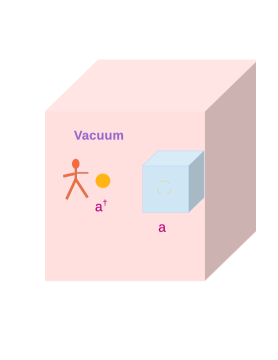
Figure 2: A schematic description of the confinement of a created particle before annihilating it. The dot (orange) presents the particle created by operator $a^{\dagger}$ and the dash circle presents its annihilation by $a$ after its confinement in the blue volume that induces a Casimir effect.

2.2 New interpretations

To better understand the physical meaning of regularization consider the operator $a_{k}a_{k}^{\dagger}+a_{k}^{\dagger}a_{k}$ in (2). The second term is the number operator $\hat{N}_{k}$ and by definition $\hat{N}_{k}|0\rangle=0|0\rangle~{}\forall~{}k$. Therefore its application does not change the state. Moreover, operationally it is well defined. the operation can be considered as creation of a particle in mode $k$ and its immediate annihilation. In a classical view these two operations are opposite to each other and leave the space unchanged if the delay between these operations is negligible. The first term is $\hat{N}_{k}+1$ and its constant part leaves a remnant energy which is the origin of the singularity in (2). This can be interpreted as an error aroused from using the classical expression of $T^{\mu\nu}$, which as explained above, in a quantum context is not well defined. In this case the operator ordering or other regularization schemes seem legitimate irrespective of the geometry of spacetime.

Regarding the operational description of energy measurement, the application of $a_{k}^{\dagger}$ creates one particle with momentum $\vec{k}$. If we exactly know the momentum of the particle, all information about its position are lost. Therefore, an observer who wants to apply the annihilation operator must first somehow localize the particle, otherwise the probability of annihilation becomes negligibly small. Such an operation would not be possible without breaking the translation symmetry of the spacetime, for instance by imposing boundaries at a distance $L\sim 1/k$ which induces a Casimir energy proportional to $1/L\sim k$, and becomes infinite for $k\longrightarrow\infty$. This shows that in contrast to some suggestions [25], the origin of Casimir energy [28, 29] is not the vacuum but the energy which is needed to break the symmetry. Fig. 2 shows a schematic description of these operations.

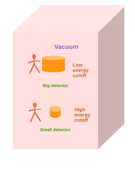
Figure 3: Schematic description of high energy cutoff on energy.

We can also interpret the energy remnant from a purely quantum mechanical point of view. A quantum field can be decomposed to $\phi(\vec{x},t)=\sum_{\{\alpha\}}u_{\{\alpha\}}(\vec{x},t)a_{\{\alpha\}}+u^{*}_{\{\alpha\}}(\vec{x},t)a_{\{\alpha\}}^{\dagger}=U(\vec{x},t)+U^{\dagger}(\vec{x},t),~{}U(\vec{x},t)\equiv\sum_{\{\alpha\}}u_{\{\alpha\}}(\vec{x},t)a_{\{\alpha\}}$. Then $\hat{T}^{00}(\vec{x},t)\propto(\dot{U}U^{\dagger}+\dot{U}^{\dagger}~{}U)(\vec{x},t)$. Operators $U$ and $U^{\dagger}$ present annihilation and creation of a particle with any momentum at a spacetime point $(\vec{x},t)$. Because the position of the created particle is exactly known, no information about its momentum can be obtained, and any value, including infinity, is allowed. These arguments are in spirit the same as those given by Eppley & Hannah [27] and in LABEL:p9 to prove the inconsistency of a classical gravity and a quantic matter. Regularization of the integral in (2) by imposing a maximum energy cutoff is equivalent to considering an uncertainty on the position. It presents the highest energy scale or equivalently smallest distances in which the observer can verify the presence of a vacuum and provides an upper limit on the vacuum energy density. See Fig. 3 for a schematic description.

2.3 Contribution of virtual particles and Standard Model condensates in dark energy

When interactions are considered, the vacuum of quantum field theory is very far from being an empty space because quantum fluctuations can condensate [30]. It is a subject of debate whether such cases should be called a vacuum or not. In any case, we cannot separate the spacetime from its quantum field content. For this reason, it is suggested that these condensates contribute to vacuum energy and thereby to dark energy [25, 31, 32]. Even in absence of condensates, loop corrections and running mass and couplings are suggested as evidence for coupling of graviton with virtual particles [31, 32], and thereby gravitational interaction of vacuum. In this case the density of dark energy should be much larger than what is observed. Thus, according to this argument the presence of a small dark energy challenges the validity of quantum field theory. Nonetheless, there are several observational facts against this criticism which are discussed in detail in [14] and can be summarized as the following:

After renormalization, the contribution of virtual particles is included in the mass and couplings of elementary particles and do not influence large scales. Moreover, renormalization is based on the removal of infinities from integrals similar to (2). The fact that after this apparently ad hoc operation we obtain relations that are confirmed by experiments, proves that these calculations are after all meaningful, see [14] for more evidence. Another indication against a gravitational interaction between free particles and vacuum is the stringent constraints on the energy dependence of dispersion relation of high energy particles during their propagation over cosmological distances [35]. This and other observations put strong constraints on the influence of quantum gravity corrections at scales much larger than Planck scale. They also constrain the recent suggestion of graviton condensation as the origin of dark energy [36], because quantum state of such a condensate would induce fluctuations in the propagation of photons proportional to their energy which are not observed. By contrast, there is no constraint on the condensate of a field without interaction with visible particles.

As for the effect of the Standard Model condensates, the most important of them is the newly discovered Higgs [37] with a nonzero vacuum expectation value (vev) of $\sim 246$ GeV. It is believed to generate mass for the Standard Model particles and triggers the breaking of $SU(2)\times U(1)$ symmetry at an scale $\gtrsim 1TeV$. The conditions for the formation of a Bose-Einstein Condensate (BEC) in a quantum fluid is studied in [38]. They demand a uniform space distribution for the field. In both classical fluid and quantum field theory the amplitude of anisotropies of a condensate decreases very rapidly for large modes. This is analogue to the infinite volume condition for symmetry breaking in statistical physics [38]. Nonetheless, in presence of additional driver, such as an interaction [34, 20], wave functions of particles and their condensate are confined to short distances. Therefore, Higgs condensate which is coupled to other particles is confined at short distances. In addition, the confinement of quarks by QCD helps to confine the Higgs condensate to small scales and it only manifests itself through the mass of particles. Similar arguments are used to show that the observed pion condensate responsible for the breaking of chiral symmetry is also confined to nucleons [39]. In Sec.4 we will show that the survival of the quintessence field condensate at cosmological scales is a consequence of its very small mass and very weak coupling that leads to the formation of a coherent state which is close to uniform at cosmological distances and survives the expansion of the Universe [20].

2.4 Vacuum as a coherent state

According to the definition of vacuum in equation (1), in the reference frame for which it is defined it does not have any particle. Therefore, we expect no effect on a particle that passes through vacuum. This property can be used as a test for the presence of a vacuum. However, quantum corrections induce an energy dependent effective mass. Therefore, it is the sensitivity of an observer to energy variation that determines how well the vacuum can be detected. An observer with a high resolution detector never sees any empty space. This means that vacuum is an abstract concept. Another issue to consider is the fact that the definition (1) is not frame independent. However, nonlocality of quantum mechanics and modification of vacuum with symmetry breaking raise the necessity for a frame independent definition for the true vacuum of quantum field theory. In this section we propose such a definition.

In [20] we have defined a generalized coherent state $|\Psi_{GC}\rangle$ for a scalar field based on an original suggestion by [40, 33]:

$$|\Psi_{GC}\rangle\equiv\sum_{k}A_{k}e^{C_{k}a_{k}^{\dagger}}|0\rangle=\sum_{k}A_{k}\sum_{i=0}^{N\rightarrow\infty}\frac{C_{k}^{i}}{i!}(a_{k}^{\dagger})^{i}|0\rangle$$ (5)

$$a_{k}|\Psi_{GC}\rangle=C_{k}|\Psi_{GC}\rangle\quad\quad\langle\Psi_{GC}|N_{k}|\Psi_{GC}\rangle=|A_{k}C_{k}|^{2}$$ (6)

For $\{C_{k}\rightarrow 0~{}\forall~{}k\}$ this state is neutralized by all annihilation operators and the expectation value of particle number approaches zero for all modes. Therefore, this state satisfies the condition (1) for a vacuum state. Coefficients $A_{k}$ are relative amplitude of modes and can be nonzero even for a vacuum state. In addition, one can extend this definition by considering products of $|\Psi_{GC}\rangle$ states. Such a state includes products of states in which particles do not have the same momentum, thus it consists of all combinations of states with any number of particles and momenta:

$$|\Psi_{G}\rangle\equiv\sum_{k_{1},k_{2},\cdots}\biggl{(}\prod_{k_{i}}A_{k_{i}}\biggr{)}e^{\sum_{i}C_{k_{i}}a_{k_{i}}^{\dagger}}|0\rangle$$ (7)

A vacuum state is defined as $C_{k_{i}}\rightarrow 0~{}\forall~{}k_{i}$ which is asymptotic limit of non-vacuum states. Under a Bogoliubov transformation this state is projected to itself:

$$a_{k_{i}}=\sum_{j}\sum_{k_{j}}{\mathcal{A}}_{k_{j}k_{i}}a^{\prime}_{k_{j}}+\sum_{j}\sum_{k_{j}}{\mathcal{B}}_{k_{j}k_{i}}{a^{\prime}}^{\dagger}_{k_{j}}\quad\quad a^{\dagger}_{k_{i}}=\sum_{j}\sum_{k_{j}}{\mathcal{A}}^{*}_{k_{j}k_{i}}{a^{\prime}}^{\dagger}_{k_{j}}+\sum_{j}\sum_{k_{j}}{\mathcal{B}}^{*}_{k_{j}k_{i}}a^{\prime}_{k_{j}}$$ (8)

Replacing $a_{k_{i}}^{\dagger}$ in (7) with the corresponding expression in (8) leads to an expression for $|\Psi_{G}\rangle$ similar to (7) but with respect to the new operator ${a^{\prime}}^{\dagger}_{k}$ and $C^{\prime}_{k_{j}}=\sum_{i}\sum_{k_{i}}{\mathcal{A}}^{*}_{k_{j}k_{i}}C_{k_{i}}$. For $C_{k_{i}}\rightarrow 0~{}\forall~{}k_{i}$ and finite ${\mathcal{A}}^{*}_{k_{j}k_{i}}$, $C^{\prime}_{k_{i}}\rightarrow 0~{}\forall~{}k_{i}$. Note that here we assume that the Bogoliubov transformation changes $|0\rangle$ to a similar state which is neutralized by $a^{\prime}_{k}~{}\forall~{}k$. Therefore, in contrast to the null state of the Fock space, $|\Psi_{G}\rangle$ is frame-independent.

It is easy to verify that this new definition of vacuum does not solve the problem of singularity of $\hat{T}^{00}$ expectation value. Nonetheless, it gives a better insight into the nature of the problem. Notably, one can use the number operator $\sum_{k}\hat{N}_{k}$ to determine the energy density of vacuum because in contrast to $|0\rangle$, the new vacuum $|\Psi_{G}\rangle$ is frame-independent and is neutralized by the number operator $\hat{N}_{k}|\Psi_{G}\rangle=0~{}\forall~{}k$. This alternative to $\hat{T}^{00}$ for measuring the vacuum energy density has been discussed in [23], but has been considered to be a poor replacement because the vacuum state defined in (1) is not frame independent. Note that we explicitly distinguish between a system in which all particles are in the ground state and a system in which the expectation value of particle number in any state, including the ground state, is zero. We call the first system a condensate and the second one according to (6) is a vacuum. Therefore, according to this definition string vacua of modulies after compactification are condensates. See [14] for more examples and details.

Although coefficients $A_{k}$ which must be calculated from the full Lagrangian depend on the initial or boundary conditions, the state $|\Psi_{G}\rangle$ contains all combinations of particles and is always projected to itself when the reference frame is changed. In this sense it is a unique maximally coherent state. Like any superposition state its observation - which needs an interaction - leads to a collapse to one of its member states. An external observer interprets this as observation of virtual particles - because they come from a presumed vacuum - and their effect manifests itself as scale dependence of mass and couplings of the field. Because any single state in the vacuum superposition has a vanishing amplitude, one can always consider that the vacuum stays unchanged even when one or any finite number of its members interact and decohere. Thus, like usual definition of vacuum, interactions modify properties of the external (untangled, on-shell) particles at scales relevant for their interaction, but they do not change $|\Psi_{G}\rangle$ globally.

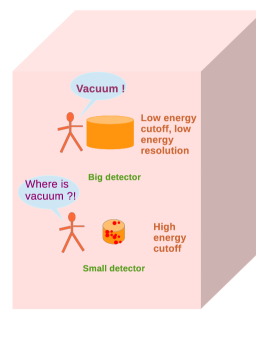
Figure 4: A schematic description of production of virtual particles by partial decoherence of vacuum. The points (red) present virtual particles which are decohered and their indirect effects can be measured by detectors as scale-dependence of mass and couplings.

The vacuum $|\Psi_{G}\rangle$ includes all states at any scale, but in every experiment only a range of them are available to observers. They are limited from IR side by the size of the apparatus or observational limits such as a horizon, and from UV side by the available energy to the observer. The presence of a particle at a given scale i.e. discrimination between vacuum and non-vacuum at that scale depends on the uncertainties in distance/energy measurements. At large distance scales the limited sensitivity of detectors cannot detect interaction with very low energy virtual particles, thus no violation of energy-momentum conservation occurs. This could not be true if the vacuum had a large energy-momentum density which could be exchanged with on-shell particles.

Does the coherent vacuum state $|\Psi_{G}\rangle$ gravitate ? A detailed answer to this question needs a quantum description for gravity. Nonetheless, by definition states that make up a coherent state are not observable except when they are decohered/collapsed. And when this happens, they will no longer appear as vacuum, see Fig. 4 for a schematic illustration. Therefore, they cannot influence observations in any way, including gravitationally. In a semi-classical view, one expects that the expectation value of the number of particles with a given energy and momentum determines the strength of the gravitational force. Equation (6) shows that this number for any mode $k$ is null when $\{C_{k}\rightarrow 0~{}\forall~{}k\}$. Thus, this state does not feel the gravity. This is another evidence of the unphysical nature of the singularity of the expectation value of energy-momentum tensor when its classical definition is used in quantum field theory without any regularization.

2.4.1 Vacuum or not Vacuum

A question which arises here is: Why does the existence of a frame-independent vacuum rule out vacuum energy as the origin of accelerating expansion ? The answer to this question depends on what we mean by vacuum. If by vacuum we mean the minimum of the effective classical - condensate - component of quantum fields, then dark energy may be considered as the vacuum energy. However, as we discussed in this section and will demonstrated in details in Sec. 4, the condensate is very far from being the particle-less state that conventional word vacuum means and the quantum state used in (1) designates. Therefore, minimums of the condensate potential should not be called vacuum. Moreover, we will show that we can begin from an initial moment where the amplitude of a condensate is zero, i.e. the state of the Universe is $|\Psi_{G}\rangle$ with $\{C_{k}\rightarrow 0~{}\forall~{}k\}$ and study its formation and evolution. These processes are also very far from the static concept of vacuum. In laboratory condensed matter the lowest energy state is usually called vacuum as synonymous to the background state above which - usually in energetic sense - fluctuations are studied. In the context of early Universe physics, the background state itself is as important and unknown as its fluctuations. Thus, employment of ambiguous terms such as vacuum only adds to confusion.

2.5 Outline

In this section, various arguments were put forward to advocate a null energy density for vacuum in the context of quantum field theories. They rule out the energy density of vacuum as the origin of dark energy. The vacuum state was shown to be an abstract concept that only approximately and asymptotically makes sense. We proposed a new frame-independent definition for vacuum as a coherent state with an amplitude approaching zero. Apart from helping to understand issues regarding the origin of dark energy, this definition may be useful for nonlocal description of quantum gravity and systems including condensates. In absence of a vacuum energy in the sense we defined here, the best candidates for dark energy are modification of the Einstein gravity and condensation of one or multiple quantum fields with quintessential behaviour.

3 Quintessence and interaction in the dark sector

3.1 Introduction

Figure 5: Rolling down of a quintessence field beginning in the early Universe and lasting up to now.

Even before the observational confirmation of an entity in the Universe behaving very similar to a cosmological constant, cosmologists have tried to find models with such behaviour at recent epochs in the history of the Universe [41]. These models are generically called Quintessence and majority of them are based on one or more scalar fields, although models based on vector fields have been also studied [42]. Similar to slow-roll models of inflation, the scalar field asymptotically approaches to the minimum of the potential at zero. In a variant of quintessence models called k-essence [43] the evolution of the scalar field is governed by the kinetic energy which has a non-standard form generally written as $K=f(\phi,\partial_{\mu}\phi)$. These models are usually inspired from string and other quantum gravity models. In some quintessence models it is considered that the same field that has generated inflation in the early Universe plays also the role of quintessence at present [44], see e.g. [45] for comparison with recent data.

It is not a trivial task to make models with what is called a tracking solution, which without fine-tuning of parameters and initial conditions for a duration more than half of the age of the Universe approaches zero without reaching to this limit point. It is shown [41, 46] that the necessary condition for the presence of such solutions is:

$$V"V/V^{\prime 2}>1$$ (9)

It is easy to verify that for analytically simple models with polynomial or exponential potentials, the condition (9) is satisfied if their order or exponent is negative. Such potentials and k-essence models are not renormalizable except when the model is linearized and only small fluctuations are quantized [93]. For this reason they must be considered as effective models. On the other hand, it is expected that a quintessence field has very weak interactions, thus its effective potential must be close to its bare potential and perturbative. This conclusion is not consistent with a nonperturbative potential.

Apart from non-renormalizability several other issues about quintessence models with only self-interaction can be remarked. As it is described in section 1, in these models the equation of state of dark energy:

$$w=\frac{P}{\rho}=\frac{\frac{1}{2}\dot{\phi}^{2}-V(\phi)}{\frac{1}{2}\dot{\phi}^{2}+V(\phi)}\geqslant-1$$ (10)

does not allow a phantom-like behaviour for positive value of the potential, and may be inconsistent with data [49]. Phantom models correspond to a Wick rotation of time coordinate in ordinary quintessence models, and are their Euclidean analogues [48]. Under this operation $\rho\rightarrow-P$, $P\rightarrow-\rho$, and $w\rightarrow 1/w<-1$. Although the Wick rotation technique is used in many circumstances in physics for simplifying calculations, usually an inverse rotation is performed at the end to bring back calculations to Lorentzian metric. In phantom models the Wick rotation is performed only in quintessence sector and it is not rotated back. Thus, it is considered that the field is in this state only for a limited time. In any case such a model can be only an effective toy model.

In addition to $w\geqslant-1$ issue, simple/pure quintessence models and a cosmological constant do not explain why the density of dark energy is fine-tuned such that galaxies could be formed before it becomes dominant. This problem is called dark energy coincidence [25]. We should remind that if the origin of dark energy is related to physics at Planck scale - as in the context of string theory - or even at lower scales such as inflation era or reheating, its density was tens of orders of magnitude smaller than matter density at early epochs. This needs an extreme fine-tuning unless there is an inherent relation between dark energy and other constituents of the Universe, for instance through an interaction between quintessence field and dark matter [50, 15, 16, 18]. Another advantage of this class of models is that they provide a natural explanation for $w_{obs}<-1$ if the interaction of dark energy with matter is ignored in analysing the data [15, 65].

We should remind that quintessence models studied in pioneering works [50] are actually modified gravity related to Brans-Dick extension of Einstein gravity. A dilaton scalar field is introduced through the transformation $g_{\mu\nu}\rightarrow e^{C\phi}g_{\mu\nu}$ in matter Lagrangian where $\phi$ is the quintessence/dilaton field, $g_{\mu\nu}$ is the metric, and $C$ a coupling constant. In [51] the couplings of dilaton to dark and baryonic matter are different. They reflect different conformal properties of these constituents and create a fifth force effect which may induce a segregation between these two types of matter. Another class of interacting quintessence models which have been extensively studied are scaling models [52, 53, 54, 55]. They assume a constant ratio of dark matter and dark energy. However, their prediction for the equation of state is $w\gtrsim-0.7$ which is inconsistent with data. Other type of scaling models based on non-standard kinetic term inspired or associated to string theory and/or brane models are also proposed [56]. In this class of models, which can be classified as k-essence, the non-standard expression of the kinetic term is due to induced metric of a 4D brane boundary by a dilaton field living in the higher dimensional bulk. Thus, the effective quintessence field on the visible brane has a geometric/gravitational origin. In our knowledge the model presented in [16, 17] is the first properly speaking interacting quintessence model with a particle physics interpretation rather than geometry.

Many extensions of the Einstein gravity and classical limit of quantum gravity models include a scalar field. The best example is $F(R)$ [57] and conformal gravity. In these models the scalar field usually has a non-minimal interaction with matter, and therefore apparently they are similar to interacting quintessence. Nonetheless, we can in principle distinguish them from their interaction, although it is a very challenging task, see Sec. 5. If like gravity, the scalar field(s) has(have) similar coupling to all type of matter, we call it modified gravity, otherwise an interacting quintessence. However, in an observational point of view it would be very difficult to test this criterion, because the scalar field is expected to have a very weak interaction with matter. Moreover, about $80\%$ of matter in the Universe is dark and cannot be observed directly. Consequently, the measurement of difference between coupling of dark energy to various component is very difficult if not impossible. For this reason other discriminating criteria should be used. This point will be discussed in detail in section 5.

3.2 Dark energy with $w_{obs}\lesssim-1$ in presence of interaction in the dark sector

Strangely enough my involvement in dark energy research began during the study of Ultra High Energy Cosmic Rays (UHECRs)! This study is summarized in Sec. LABEL:sec:he-uhecr. Here we just mention that to verify the consistency of a decaying super-heavy dark matter as the origin of UHECRs in the context of top-down models, in [15] the evolution of Hubble function $H(z)$ in these models is compared with the available set of data from supernovae type Ia [59, snpro, 62] for various lifetime of dark matter. In a flat universe with a cosmological constant $H(z)$ is:

$$H^{2}(z)=\frac{8\pi G}{3}T^{00}(z)+\frac{\Lambda}{3}$$ (11)

where $T^{\mu\nu}$ is the energy-momentum tensor. For stable matter and radiation $T^{00}(z)=\rho_{c}\Omega_{m}(1+z)^{3}+\Omega_{h}(1+z)^{4}$ where $\rho_{c}\equiv 3H_{0}^{2}/8\pi G$ is the present critical density, $\Omega_{m}$ and $\Omega_{h}$ are fractional density of cold and hot matter, respectively, and $z$ is the redshift. When dark matter decays or interacts with other components [65], there is no exact expression for $T^{00}$ because it depends on the decay modes of the meta-stable dark matter, its elastic and non-elastic couplings, and the fate of remnants i.e. whether they are and stay relativistic or lose their energy and become non-relativistic. For this reason numerical simulations of the decay of a super-heavy dark matter which includes the propagation and dissipation of its remnants is used to determine $T^{00}$.

Fig. 6 shows the best fit of data with simulations. The data used in [15] is the published data set B of the Supernova Cosmology Project [59, 60, 61] for high redshift and Calan-Tololo sample [58] for low redshift supernovae. It should be reminded that $w_{m}$ the equation of state of matter for a decaying/interacting dark matter is not null, i.e. it is not an ideal Cold Dark Matter (CDM) with $w_{m}=0$. This is an important point because it is this difference that leads to equation state of dark energy $w_{de}\lesssim-1$ if the decay or interaction of dark matter is not taken into account in the model fitted to the data. We call the value of $\Omega_{\Lambda}$ and $w_{de}$ derived with the assumption of a stable dark matter $\Omega_{\Lambda}^{eq}$ and $w_{de}^{eq}$. These values should be compared with what is in the literature because their null hypothesis is usually a stable CDM.

Figure 6: Best fit residues of apparent magnitude of supernovae for $\Omega_{\Lambda}^{eq}=0.7$, $\tau=5\tau_{0}$, where $\tau_{0}$ is the present age of the Universe and $\tau$ the lifetime of dark matter in simulations. The value of fractional cosmological constant density used in this simulation is $\Omega_{\Lambda}=0.73$ (full line). Other curves are for stable dark matter with $\Omega_{\Lambda}^{eq}=\Omega_{\Lambda}=0.7$ (doted); decaying dark matter with $\tau=5\tau_{0}$ and $\Omega_{\Lambda}=0$ (dash line); stable DM and $\Omega_{\Lambda}=0$ (dash-dot).

Additionally, for each model of decaying dark matter and a cosmological constant as dark energy we determined parameters of an equivalent quintessence model with stable dark matter and density $\rho_{q}=\Omega_{q}(1+z)^{3(w_{q}+1}$. Fig. 7 shows the variation of $\chi^{2}$ of the fit with $w_{q}$. Table 1 shows the value of parameters for the equivalent quintessence models. Regarding the value of $\chi^{2}$ of these models, they are all consistent with data. However, clearly models with $w_{q}<-1$ fit the data somehow better, except the model with $\Omega_{\Lambda}=0.8$ which has a poorer fit than others. This proves that the wrong priory of a stable or non-interacting matter can lead to $w_{q}<-1$ when dark matter decays or interacts and dark energy is a cosmological constant. This work is one of the first work in which it was shown that the observed $w<-1$ for dark energy can be due to the application of a wrong model. Results shown in Fig. 7 and Table 1 are consistent with latest measurements of the equation state of dark energy from supernova data [63], LSS, and CMB anisotropies [49].

Figure 7: $\chi^{2}$-fit of supernovae data with quintessence models as a function of $w_{q}$ for $\Omega_{q}=0.67$ (dashed), $\Omega_{q}=0.69$ (dash-dot), $\Omega_{q}=0.71$ (solid) and $\Omega_{q}=0.8$ (dotted). $\chi^{2}$’s of equivalent quintessence models to a decaying dark matter with $\tau=5\tau_{0}$ and closest $\Omega_{\Lambda}$ to $\Omega_{q}$ (see table 1) are also shown. $\tau$ and $\tau_{0}$ are respectively the lifetime of dark matter in simulations and the present age of the Universe. Except $\Omega_{q}=0.8$ model others are all good fits to data. For $\Omega_{\Lambda}=\Omega_{q}=0.8$, a stable DM fits the data better, but the fit is poorer than former models.

	Stable DM			$\tau=50\tau_{0}$			$\tau=5\tau_{0}$
	$\Omega_{\Lambda}=0.68$	$\Omega_{\Lambda}=0.7$	$\Omega_{\Lambda}=0.72$	$\Omega_{\Lambda}=0.68$	$\Omega_{\Lambda}=0.7$	$\Omega_{\Lambda}=0.72$	$\Omega_{\Lambda}=0.68$	$\Omega_{\Lambda}=0.7$	$\Omega_{\Lambda}=0.72$
$H_{0}$	$69.953$	$69.951$	$69.949$	$69.779$	$69.789$	$69.801$	$68.301$	$68.415$	$68.550$
$\Omega_{\Lambda}^{eq}$	$0.681$	$0.701$	$0.721$	$0.684$	$0.704$	$0.724$	$0.714$	$0.733$	$0.751$
$\Omega_{q}$	-	-	-	$0.679$	$0.700$	$0.720$	$0.667$	$0.689$	$0.711$
$w_{q}$	-	-	-	$-1.0066$	$-1.0060$	$-1.0055$	$-1.0732$	$-1.0658$	$-1.0590$
$\chi^{2}$	$62.36$	$62.23$	$62.21$	$62.34$	$62.22$	$62.21$	$62.22$	$62.15$	$62.20$

Table 1: Cosmological parameters from simulations of a decaying DM and parameters of the equivalent quintessence models. $H_{0}$ is in $km$ $Mpc^{-1}\sec^{-1}$.

It is well known that simulations and fitting include many approximations and uncertainties. To prove that the conclusion about the effect of neglecting decay/interaction of dark matter on the measured value of $w$ is not an artifact, in [15] an approximate analytical demonstration was also performed. Due to the importance of this demonstration for our understanding of observations and models it is summarized here:

3.2.1 Analytical demonstration

With a good precision the total density of a decaying dark matter model can be written as the following:

$$\frac{\rho(z)}{{\rho}_{c}}\approx{\Omega}_{m}(1+z)^{3}\exp(\frac{{\tau}_{0}-t}{\tau})+{\Omega}_{hot}(1+z)^{4}+{\Omega}_{m}(1+z)^{4}\biggl{(}1-\exp(\frac{{\tau}_{0}-t}{\tau})\biggr{)}+{\Omega}_{\Lambda}.$$ (12)

where $\rho_{c}$ is the critical density of the Universe at redshift zero and ${\Omega}_{hot}$ is the fractional density of relativistic components. It is assumed that decay remnants are relativistic particles and their dissipation is neglected. In a flat cosmology ${\Omega}_{m}+{\Omega}_{hot}+{\Omega}_{\Lambda}=1$ and ${\rho}_{c}$ is the present critical density. If dark matter is stable and we neglect the contribution of hot dark matter, the expansion factor $a(t)$ is:

$$\frac{a(t)}{a({\tau}_{0})}=\biggl{[}\frac{(B\exp(\alpha(t-{\tau}_{0}))-1)^{2}}{4AB\exp(\alpha(t-{\tau}_{0}))}\biggr{]}^{\frac{1}{3}}\equiv\frac{1}{1+z}.$$ (13)

$$A \equiv \frac{{\Omega}_{\Lambda}}{1-{\Omega}_{\Lambda}},$$ (14)

$$B \equiv \frac{1+\sqrt{{\Omega}_{\Lambda}}}{1-\sqrt{{\Omega}_{\Lambda}}},$$ (15)

$$\alpha \equiv 3H_{0}\sqrt{{\Omega}_{\Lambda}}.$$ (16)

Using (13) as an approximation for $\frac{a(t)}{a({\tau}_{0})}$ when dark matter slowly decays, (12) takes the following form:

$$\frac{\rho(z)}{{\rho}_{c}} \approx {\Omega}_{m}(1+z)^{3}C^{-\frac{1}{\alpha\tau}}+{\Omega}_{hot}(1+z)^{4}+{\Omega}_{m}(1+z)^{4}(1-C^{-\frac{1}{\alpha\tau}})+{\Omega}_{\Lambda}.$$ (17)

$$C \equiv \frac{1}{B}\biggl{(}1+\frac{4A}{(1+z)^{3}}-\sqrt{(1+\frac{4A}{(1+z)^{3}})^{2}-1}\biggr{)}.$$ (18)

For a slowly decaying dark matter, $\alpha\tau\gg 1$ and (17) becomes:

$$\frac{\rho(z)}{{\rho}_{c}} \approx {\Omega}_{m}(1+z)^{3}+{\Omega}_{hot}(1+z)^{4}+{\Omega}_{q}(1+z)^{3{\gamma}_{q}},$$ (19)

$${\Omega}_{q}(1+z)^{3{\gamma}_{q}} \equiv {\Omega}_{\Lambda}(1+\frac{{\Omega}_{m}}{\alpha\tau{\Omega}_{\Lambda}}z(1+z)^{3}\ln C).$$ (20)

Equation (20) is the definition of equivalent quintessence component. After its linearization:

$$w_{q}\equiv{\gamma}_{q}-1\approx\frac{{\Omega}_{m}(1+4A)(1-\sqrt{2A})}{3\alpha\tau{\Omega}_{\Lambda}B}-1.$$ (21)

It is easy to see that in this approximation $w_{q}<-1$ if ${\Omega}_{\Lambda}>\frac{1}{3}$.

3.3 Quintessence from decay of a super-heavy dark matter

Motivated by the arguments given in section 3 in favour of an interacting quintessence model, a model with a slowly disintegrating dark matter is considered which has a very weak interaction with a light scalar considered to be the quintessence field [16]. Furthermore, through the study of this class of models, some of advantages of an interaction in the dark sector are shown.

Consider that just after inflation the Universe consists of a cosmological soup including 2 species: a superheavy dark matter (SDM) called $X$ which is decoupled from the rest of the soup since very early times, and the ensemble of other species which we do not specify in detail. The only constraint imposed on the latter component is that it must consist of light species in - comparison with $X$ - including: baryons, neutrinos, photons, and light dark matter. For simplicity we assume that $X$ is a scalar field ${\phi}_{x}$ and is meta-stable, i.e. it decays with a lifetime much longer than the present age of the Universe. A very small energy fraction of the decay remnants is transferred to a light scalar quintessence field ${\phi}_{q}$ with negligibly weak interaction with other fields. This model is motivated by top-down models for the origin of Ultra High Energy Cosmic Rays [66, 67, 68, 69, 70, 71, 18]. Despite recent arguments against this type of models [73, 72], they are not yet completely ruled out. And even if it turns up that UHECRs have astronomical origin, dark matter or one of its constituents can be meta-stable, see e.g. [74, 72]. Remind that smaller the fraction of this type of particles in the dark matter, shorter their lifetime and larger their coupling to the quintessence field are allowed [71].

The effective Lagrangian of this model is:

$${\mathcal{L}}=\int d^{4}x\sqrt{-g}\biggl{[}\frac{1}{2}g^{\mu\nu}{\partial}_{\mu}{\phi}_{x}{\partial}_{\nu}{\phi}_{x}+\frac{1}{2}g^{\mu\nu}{\partial}_{\mu}{\phi}_{q}{\partial}_{\nu}{\phi}_{q}-V({\phi}_{x},{\phi}_{q},J)\biggr{]}+{\mathcal{L}}_{J}$$ (22)

The field $J$ presents collectively light particles. The term $V({\phi}_{x},{\phi}_{q},J)$ comprises all interactions including self-interaction potentials for ${\phi}_{x}$ and ${\phi}_{q}$:

$$V({\phi}_{x},{\phi}_{q},J)=V_{q}({\phi}_{q})+V_{x}({\phi}_{x})+g{{\phi}_{x}}^{m}{{\phi}_{q}}^{n}+W({\phi}_{x},{\phi}_{q},J)$$ (23)

The term $g{{\phi}_{x}}^{m}{{\phi}_{q}}^{n}$ is important because it is responsible for the annihilation of $X$ and back reaction of quintessence field. $W({\phi}_{x},{\phi}_{q},J)$ presents other interactions which contribute to decay of $X$ to light fields $J$ and ${\phi}_{q}$. To determine the evolution of these fields we consider $X$ and $J$ as classical particles. The contribution of quintessence field ${\phi}_{q}$ consists of classical relativistic particles with density $\rho^{\prime}_{q}$ and a condensate component behaving as dark energy with density $\rho_{q}$. Under these simplifying assumptions, the evolution equations of various components of the model are written as the followings:

$$\dot{{\phi}_{q}}[\ddot{{\phi}_{q}}+3H\dot{{\phi}_{q}}+{m_{q}}^{2}{\phi}_{q}+\lambda{{\phi}_{q}}^{3}] = -2g\dot{{\phi}_{q}}{\phi}_{q}\biggl{(}\frac{2{\rho}_{x}}{{m_{x}}^{2}}\biggr{)}+{\Gamma}_{q}{\rho}_{x}$$ (24)

$$\dot{{\rho}_{x}}+3H{\rho}_{x} = -({\Gamma}_{q}+{\Gamma}_{J}){{\rho}_{x}}-{\pi}^{4}g^{2}\biggl{(}\frac{{{\rho}_{x}}^{2}}{{m_{x}}^{3}}-\frac{{{\rho}_{q}}^{\prime 2}}{{m_{q}}^{3}}\biggr{)}$$ (25)

$$\dot{{\rho}_{J}}+3H({\rho}_{J}+P_{J}) = {\Gamma}_{J}{{\rho}_{x}}$$ (26)

$$H^{2} \equiv \biggl{(}\frac{\dot{a}}{a}\biggr{)}^{2}=\frac{8\pi G}{3}({\rho}_{x}+{\rho}_{J}+{\rho}_{q})$$ (27)

$${\rho}_{q} = \frac{1}{2}{m_{q}}^{2}{\dot{{\phi}_{q}}}^{2}+\frac{1}{2}{m_{q}}^{2}{{\phi}_{q}}^{2}+\frac{\lambda}{4}{{\phi}_{q}}^{4}$$ (28)

The constants ${\Gamma}_{q}$ and ${\Gamma}_{J}$ are respectively the decay width of $X$ to ${\phi}_{q}$ and to other species. The effect of decay term $W({\phi}_{x},{\phi}_{q},J)$ in the Lagrangian appears as the total decay rate of $X$ particles $({\Gamma}_{q}+{\Gamma}_{J}){\rho}_{x}$ in energy conservation equation. The effect of $g$-coupling is considered separately.

The system of equations (24)-(28) is highly non-linear and an analytical solution cannot be found easily. There are however two asymptotic regimes which permit an approximate analytical treatment. The first solution corresponds to early times just after the production of $X$ particles, presumably after preheating [75]) [77, 78, 79]. In this epoch ${\phi}_{q}\sim 0$ and can be neglected. The other regime is when the time variation of ${\phi}_{q}$ becomes very slow and one can neglect $\ddot{{\phi}_{q}}$. In [16] it is shown that these regimes can be connected smoothly and the final solution is very close to a constant, i.e. the quintessence field imitates a cosmological constant.

Numerical solution of equations (24) to (28) confirms the above approximate analytical conclusions. Fig. 8 presents the results of the numerical calculation of the evolution of the density of quintessence field in this type of models. We conclude that for a large fraction of the parameter space and without fine-tuning, the scalar field varies very slowly soon after beginning of its formation, and behaves similar to a cosmological constant.

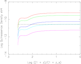
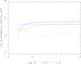
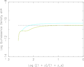
Figure 8: Evolution of the density of quintessence field. Left: for various values of energy fraction of dark matter decay remnants transformed into quintessence field: $10^{-16}$ (magenta), $5\times 10^{-16}$ (cyan), $10^{-15}$ (blue), $5\times 10^{-15}$ (green), $10^{-14}$ (red). The mass and self-coupling of the field quintessence are respectively $10^{-6}$eV and $10^{-20}$; Center: for different values of quintessence mass $10^{-3}$eV (cyan), $10^{-5}$eV (magenta), $10^{-6}$eV (red) and $10^{-8}$eV (green); Right: for different values of self-coupling: $10^{-10}$ (cyan), $10^{-15}$, $10^{-20}$ and $10^{-25}$ (green). The difference between the density of quintessence field for the last 3 values of self-coupling is smaller than the resolution of this figure. The dash line is the observed value of the density of energy dark. $z_{s}$ is the redshift after which the density of condensate remains constant up to resolution of simulations.

3.3.1 Perturbations

Due to clustering of matter, an interaction in the dark sector can apriori induce a clustering in dark energy. However, there are stringent constraints on the anisotropic expansion of the Universe [80] and clustering of dark energy [81]. Therefore, it is necessary to verify that the model described above predicts an enough uniform distribution for the quintessence field to be consistent with data.

After describing Einstein and Boltzmann equations for the scalar metric perturbations, linear perturbations of various matter components of this model, and few approximations to make an analytical calculation possible, we find the following relation between spatial fluctuation of quintessence field $\delta{\phi}_{q}$ and velocity dispersion of dark matter $\delta{u_{x}}^{i}$:

$$-V^{\prime}(\bar{{\phi}_{q}},\bar{\rho}_{x}){\partial}^{i}(\delta{\phi}_{q})={\Gamma}_{q}\bar{\rho}_{x}\delta{u_{x}}^{i}$$ (29)

This equation shows that the divergence of quintessence field fluctuations ${\partial}^{i}\delta{\phi}_{q}$ follows the velocity dispersion of dark matter in opposite direction. However, its amplitude is largely reduced due to the very small decay width ${\Gamma}_{q}$. In addition, with the expansion of the Universe, $V^{\prime}(\bar{{\phi}_{q}},\bar{\rho}_{x})$ varies only very slightly, i.e. just the interaction between SDM and ${\phi}_{q}$ changes. In contrast, $\bar{\rho}_{x}$ decreases by a factor of $a^{-3}(t)$ and even a gradual increase in the dark matter clumping and its velocity dispersion $\delta{u_{x}}^{i}$ is not enough to compensate the effect of its decreasing density [81]. Therefore, we conclude that the spatial variation of ${\phi}_{q}$ is very small and unobservant.

Finally, for testing this class of models against data, in addition to their impact on the expansion of the Universe and clustering that will be discussed in more detail in Sec. 5, there are other means which can be used. In particular, a decaying heavy dark matter produces relativistic remnants which should be detectable directly if they are visible particles, or indirectly - through their effect on the evolution of large structure - if they are invisible. In fact some of recent observations prefer a larger number of relativistic species - usually described as the effective number of neutrinos [82], which apriori can be related to decay or interaction of dark matter. However, there are other explanations for these observations, for instance the existence of one or two sterile neutrinos [83]. Therefore, for the time being it is not possible to make a conclusion.

Alternatively, the lifetime of the decaying dark matter can be short. In this case, it has decayed longtime ago. Nonetheless, as we discussed before, the potential of quintessence field after its saturation stays constant and behave as a cosmological constant. This can explain the extreme fine-tuning of dark energy density with respect to dark matter in the early Universe. On the other hand, at late times the accelerating expansion of the Universe can destroy the coherence of quintessence condensate and dilute it. The study of this issue in the framework of quantum field theory is explained in the next section.

4 Condensation of a quantum scalar field as the origin of dark energy

4.1 Introduction

Quintessence models and many other phenomena in cosmology, particle physics, and condensed matter are associated to scalar fields which at large scales behave classically. Classical scalar fields have been first introduced in the fundamental physics in the framework of extensions to Einstein gravity [84, 85], and as a means for unification of gravity with other forces [86, 87]. They can be related to gravity models with conformal symmetry and its breaking which generates a scalar-tensor gravity [88]. Thus, in these models the scalar field has a geometrical origin, at least at energy scales much smaller than Planck mass. By contrast, other known scalar fields such as Higgs in the Standard Model or Cooper pairs in condensed matter have a quantic point-like/particle nature, which has been experimentally demonstrated in both particle physics [89] and condensed matter [90] . Their classical behaviour is associated to a special quantum state called a condensate - in analogy with condensation of droplets of liquid from particles or molecules of a vapor. In this section we briefly describe how a condensate can be formed at cosmological scales [20, 92, 91].

Decoherence of a scalar field due to its interaction with an environment, and the settlement of particles in one of the two minimum of a double-well potential is suggested as the origin for a nonzero vacuum energy and a prototype for landscape of string models [93, 94]. This looks like counter intuitive because apriori the decoherence should reduce quantum correlations. In fact, it is exactly what happens. Rather than being in a quantum superposition of many energy states, by forming a condensate the energy distribution of particles is limited to one or few energy levels, see e.g. [95]. Although a condensate is a superposition state, it is more deterministic, i.e. has a smaller entropy, than the quantum state from which it is formed.

The formation of a condensate in cosmological environment raises several additional complexities, because the condensate must have an extension comparable to the size of the Universe. First of all, the mass of the scalar field and its coupling, both self and to other fields, must be very small. In the framework of the model explained in the previous section, quintessence particles are produced by the decay of a heavy particle. Consequently, at the moment of their production they must be highly relativistic. For instance, if they are produced during preheating after inflation or even at higher energy scales - for instance if they are associated to modulies in string theory - they must be initially relativistic. In laboratory, particles destined for condensation are usually cooled to very low temperatures before the process of condensation can occur. Due to their very weak coupling, quintessence particles cannot easily cool. These facts put stringent constraints on the condensation of a scalar field. Therefore, a comprehensive study is necessary to see whether a condensation can arise and to determine the necessary conditions for its occurrence. The first results of such an investigation are reported in [20, 92, 91].

In quantum mechanics, expectation values of hermitian operators associated to observables present the outcome of measurements. Therefore, it is natural to define the classical observable (component) of a quantum scalar field as its expectation value:

$$\varphi(x)\equiv\langle\Psi|\Phi(x)|\Psi\rangle\neq 0$$ (30)

where $|\Psi\rangle$ is an element of the Fock space of the system. It is easily seen that a coherent state consisting of the superposition of indefinite number of particles in a single quantum state - presumably the ground state - behaves like a classical field as defined in (30) i.e. $\langle\Psi|\Phi(x)|\Psi\rangle\neq 0$ [33]. On the other hand, bosonic particles occupying the same energy state form a Bose-Einstein condensate. For this reason, the classical field $\varphi(x)$ is called a condensate. Using canonical representation, it is easy to see that for a limited number of free scalar particles $\langle\Psi|\Phi|\Psi\rangle=0$. Nonetheless, in presence of an interaction, after renormalization a finite term can survive even when the state has a finite number of particles [96]. In this case, the field $\Phi$ can be considered to be dressed, which effectively presents an infinite number of virtual particles and satisfies the condensation condition [97]. In such cases, the expectation value can be non-zero even on the vacuum.

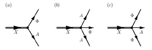
Figure 9: Decay models of heavy dark matter $X$.

4.1.1 Formation of a quantum quintessence field

To investigate the reliability of quintessence models in a quantum field theoretical point of view, we consider a phenomenological model similar to one explained in Sec. 3. The model consists of a heavy particle $X$ slowly decaying to two types of particles: a light scalar $\Phi$ and another field $A$ which can be an intermediate state or a collective notation for other fields. Here for simplicity it is assumed to be a scalar too. The particle $X$ and one of the remnants can be spinors, but the quintessence field $\Phi$ however must be a scalar. In the extreme density of the Universe after reheating, apriori the formation of Cooper-pair composite scalars from fermions is possible. However, this process needs a relatively strong interaction between fermions, and can arise in local phenomena such as Higgs mechanism and leptogenesis. But, due to very weak interaction of dark energy this does not seem to be plausible for $\Phi$. The simplest decay modes are shown in Fig. 9.

Diagram (9-a) is the simplest decay/interaction mode. Diagram (9-b) is a prototype decay mode when $X$ and $\Phi$ share a conserved quantum number or $A$ and $\bar{A}$ (here $A=\bar{A}$ is considered) have a conserved quantum number. For instance, one of the favorite candidates for $X$ is a (s)neutrino decaying to a much lighter (pseudo-)scalar field and another (s)neutrino carrying the same leptonic number [98]. With seesaw mechanism between superpartners, a mass split between right and left (s)neutrinos, respectively corresponding to $X$ and $\Phi$, can occur. Depending on the conservation or violation of $R$-symmetry, the other remnant can be another scalar superpartner, Higgs or Higgsino.

The Lagrangian of this model is:

$${\mathcal{L}} = {\mathcal{L}}_{\Phi}+{\mathcal{L}}_{X}+{\mathcal{L}}_{A}+{\mathcal{L}}_{int}$$ (31)

$${\mathcal{L}}_{\Phi} = \int d^{4}x\sqrt{-g}\biggl{[}\frac{1}{2}g^{\mu\nu}{\partial}_{\mu}\Phi{\partial}_{\mu}\Phi-\frac{1}{2}m_{\Phi}^{2}{\Phi}^{2}-\frac{\lambda}{n}{\Phi}^{n}\biggr{]}$$ (32)

$${\mathcal{L}}_{X} = \int d^{4}x\sqrt{-g}\biggl{[}\frac{1}{2}g^{\mu\nu}{\partial}_{\mu}X{\partial}_{\mu}X-\frac{1}{2}m_{X}^{2}X^{2}\biggr{]}$$ (33)

$${\mathcal{L}}_{A} = \int d^{4}x\sqrt{-g}\biggl{[}\frac{1}{2}g^{\mu\nu}{\partial}_{\mu}A{\partial}_{\mu}A-\frac{1}{2}m_{A}^{2}A^{2}-\frac{\lambda^{\prime}}{n^{\prime}}A^{n^{\prime}}\biggr{]}$$ (34)

$${\mathcal{L}}_{int} = \int d^{4}x\sqrt{-g}\begin{cases}\mathsf{g}\Phi XA,&\text{For (\ref{decaymode})-a}\\ \mathsf{g}\Phi XA^{2},&\text{For (\ref{decaymode})-b}\\ \mathsf{g}{\Phi}^{2}XA,&\text{For (\ref{decaymode})-b}\end{cases}$$ (35)

In the rest of this section we only describe the case (a) in detail. Note that no self-interaction is considered for $X$. The self-interaction of $A$ can be an effective description for interaction of fields collectively presented by $A$. Very weak interaction constraint on dark energy means that couplings $\lambda$ and $\mathsf{g}$ must be very small. In a realistic particle physics model, renormalization and non-perturbative effects can lead to complicated potentials for scalar fields. An example relevant to dark energy is a pseudo-Nambu-Goldstone boson field with a shift symmetry [99] which protects the very small mass of the quintessence field. The power-law potential considered in (32) can be interpreted as the dominant term or one of the terms in a potential with shift symmetry.

4.2 Decomposition and evolution equations

As we discussed above, our main aim is to study the evolution of quintessence condensate. Following definition (30) we decompose $\Phi(x)$ to a condensate and a quantum component:

$$\Phi(x)=\varphi(x)I+\phi(x)\quad\quad\langle\Phi\rangle\equiv\langle\Psi|\Phi|\Psi\rangle=\varphi(x)\quad\quad\langle\phi\rangle\equiv\langle\Psi|\phi|\Psi\rangle=0$$ (36)

where $I$ is the unit operator. We remind that in (36) both classical and quantum components depend on the spacetime $x$. We do not assume a homogeneous Universe, but only consider small anisotropies. We assume $\langle X\rangle=0$ and $\langle A\rangle=0$. The justification for these assumptions is the large mass and perturbative interactions of $X$ and $A$ which reduce their number and quantum effects. Later we show quantitatively that when the mass of a field is large, the minimum of effective potential of its condensate approaches zero. As $X$ and $A$ have a very weak interaction with $\Phi$, their evolution can be studied semi-classically by using the Boltzmann equation with a collisional term [71, 16]. A more precise formulation should use the full Schwinger-Keldysh / Kadanoff-Baym formalism. This is a work in progress [100].

After insertion of decomposition (36) into the Lagrangian (31), the evolution equation for the condensate $\varphi$ with interaction (a) is obtained by application of variational principle:

$$\frac{1}{\sqrt{-g}}{\partial}_{\mu}(\sqrt{-g}g^{\mu\nu}{\partial}_{\nu}\varphi)+m_{\Phi}^{2}\varphi+\frac{\lambda}{n}\sum_{i=0}^{n-1}(i+1)\binom{n}{i+1}{\varphi}^{i}\langle{\phi}^{n-i-1}\rangle-\mathsf{g}\langle XA\rangle=0\quad\quad\text{for (\ref{decaymode}-a)}$$ (37)

Note that in (35) non-local interactions, i.e. terms containing derivatives of $\varphi$ do not contribute in the evolution of $\varphi$ because they are all proportional to $\phi$. After taking expectation value of the operators they cancel out because $\langle\phi\rangle=0$ by definition. The expectation values depend on the quantum state of the system $|\Psi\rangle$ which presents the state of all particles in the system. We should remind that the mass of quantum component $\phi$ and thereby its evolution depends on $\varphi$. Moreover, through the interaction of $\Phi$ with $X$ and $A$ evolution of all the constituents of this model are coupled. In fact, for $n\geqslant 2$ the expectation values $\langle\phi^{(n-i-1)}\rangle~{}~{}i=0,\cdots,n-1$ modify the mass and self-coupling of $\varphi$. Another important observation is that in general, the effective potential of condensate $\varphi$ is not the same as the classical potential in the Lagrangian.

(38)

(39)

(40)

Figure 10: Diagrams included in the calculation of expectation values for decay model (a). The dash line presents the condensate component $\varphi$.

We use Schwinger-Keldysh closed time path integral formalism to calculate expectation values in (37) at zero-order (tree diagrams). The next relevant diagram is of order $g^{3}$, see Fig. 10. Therefore, under the assumption of the small couplings for the quintessence field, higher order diagrams are negligible. The decomposition of $\Phi$ also affects the renormalization of the model. This issue has been already studied [96] and we do not consider it here. We simply assume that masses and couplings in the model have their values after renormalization. One reason for overlooking this issue is the fact that it should be discussed in the context of a full particle physics model. In accordance with the decomposition (36), the sum of graphs in (40) is null because they correspond to the field equation of $\varphi$ (37). Finally, the expectation values at zero order are:

$$\langle XA\rangle_{a} = -i\mathsf{g}\int\sqrt{-g}d^{4}y\varphi(y)\biggl{[}G_{A}^{>}(x,y)G_{X}^{>}(x,y)-G_{A}^{<}(x,y)G_{X}^{<}(x,y)\biggr{]}$$ (41)

$$\langle\phi^{i}\rangle = -i\lambda\int\sqrt{-g}d^{4}y\varphi^{n-i}(y)\biggl{[}[G_{\phi}^{>}(x,y)]^{i}-[G_{\phi}^{<}(x,y)]^{i}\biggr{]}$$ (42)

where $G^{>}$ and $G^{<}$ are respectively advanced and retarded propagators, related to the Feynman propagator $G_{F}(x,y)=G^{>}(x,y)\Theta(x^{0}-y^{0})+G^{<}(x,y)\Theta(y^{0}-x^{0})$ which can be determined by solving following field equations:

$$\frac{1}{\sqrt{-g}}{\partial}_{\mu}(\sqrt{-g}g^{\mu\nu}{\partial}_{\nu}G^{\phi}_{F}(x-y))+(m_{\Phi}^{2}+(n-1)\lambda{\varphi}^{n-2})G^{\phi}_{F}(x-y)=-i\frac{{\delta}^{4}(x-y)}{\sqrt{-g}}$$ (43)

$$\frac{1}{\sqrt{-g}}{\partial}_{\mu}(\sqrt{-g}g^{\mu\nu}{\partial}_{\nu}G^{i}_{F}(x-y))+m_{i}^{2}G^{i}_{F}(x-y)=-i\frac{{\delta}^{4}(x-y)}{\sqrt{-g}}\quad,\quad i=X,A$$ (44)

It is remarkable that even at zero (classical) order $G^{\phi}_{F}(x-y)$ depends on the condensate field $\varphi$. The coupling between quantum component $\phi$ and the condensate $\varphi$ is the origin of the back-reaction of the condensate formation on the quantum fields. Assuming that $\Phi$ particles are produced only through the decay of $X$, the initial value of $\varphi=0$ and the coupling between $\phi$ and $\varphi$ is very small. With the growth of the $\varphi$ amplitude, the effective mass of $\phi$ particles increases. In turn, this affects the growth of the condensate because due to an energy barrier $\phi$ particles will not be able to join the condensate anymore. This negative feedback prevents an explosive formation of the condensate. We should remind that for a full consideration of the backreaction of interactions we must consider propagators that include 2-Particle Irreducible (2-PI) self-energy correction. However, their inclusion makes the problem completely unsolvable analytically. For this reason the full formulation is left for a future work [100] that will study this model through numerical simulations.

We expect a rapid decoherence of $\phi$ particles and other species due to the fast acceleration of the Universe. It pushes long wavelength fluctuations (IR modes) out of the horizon. In turn, they play the role of an environment for the decoherence of shorter modes. Thus, $X$, $A$, and $\phi$ particles can be considered as semi-classical and the evolution of their density is ruled by classical Boltzmann equations, see e.g. [71]. A complete treatment of the model as a non-equilibrium quantum process must include Kadanoff-Baym equations. It would be necessary when this model is studied in the context of a realistic particle physics.

The last set of equations to be considered for a consistent and full solution of the model are Einstein equations that determine the relation between the geometry of the spacetime and the evolution of its matter content. Apriori it is important to consider the backreaction of matter and dark energy anisotropies on the metric, at least in linear order which is a good approximation at large scales even today. However, due to the complexity of the model, we only consider a homogeneous background metric. It is shown in [20] that at linear order propagators in a background with small scalar fluctuations are simply $G_{h}(x,y)(1+\psi)$ where $\psi$ is the gravitational potential in the Newtonian gauge and $G_{h}(x,y)$ is the propagator in a homogeneous background. This relation can be used to estimate the effect of metric fluctuations on the evolution of quintessence condensate. Under these approximations only the evolution of expansion factor $a(t)$, i.e. the Friedmann equation has special importance for the determination of condensate evolution.

During radiation domination epoch the density of non-relativistic particles such as $X$ is by definition negligible, and evolution of $a(t)$ is governed by relativistic species which are not considered here explicitly. From the observed density of dark energy we can conclude that in this epoch its density was much smaller than other components, and had negligible effect on the evolution of expansion factor. In the matter domination epoch both $X$ and $A$ are assumed to be non-relativistic. If the lifetime of $X$ is much shorter than the age of the Universe at the beginning of matter domination epoch, most of $X$ particles have decayed, and $X$ does not play a significant role in the evolution of $a(t)$ which is determined by other non-relativistic species. If the lifetime of $X$ is much larger than the age of the Universe, then $X$ particles can have a significant contribution in the total density of matter. Considering the very slow decay of $X$, in the calculation of $a(t)$, at lowest order it can be approximately treated as stable and $a(t)$ evolves similar to the case of a CDM model. A better estimation of $a(t)$ can be obtained by taking into account the decay of $X$ to relativistic particles [15]. Once again here we use the simplest approximation because the problem in hand is very complicated and we want to keep the evolution of $a(t)$ decoupled from other equations such that we can obtain an analytical approximation. At late times when the density of the condensate becomes comparable to matter density, the full theory including Boltzmann equations must be solved. In this case the evolution of $a(t)$ is closely related to the evolution of the quintessence condensate and a full numerical solution is necessary.

4.3 Quantum state

Propagators and expectation values described in the previous section are defined for the quantum state of constituents of the Universe content. Therefore, before any attempt to calculate these quantities we must know their quantum state.

Due to weak interactions between particles in this model, after their decoherence they can be considered as freely-scattering particles, and therefore their quantum state $|\Psi_{f}\rangle$ can be approximated by direct multiplication of single particle states:

$$|\Psi_{f}\rangle=\sum_{p_{j}}\bigotimes_{i,j}f^{i}(x,\{p_{j}\},\varphi)|p^{i}_{j}\rangle$$ (45)

The indices $i$ and $j$ respectively present the species type and particle number, and $\{p_{j}\}$ the momentum of all states. Distributions $f^{i}(x,\{p_{j}\},\varphi)$ can be related to quantum properties of the system by using Wigner function [101]. Note that due to the dependence of masses and couplings on the condensate $\varphi$, distribution of semi-classical particles depend on this quantity too. By projecting $\Psi$ into the coordinate space we can express $|\Psi|^{2}$ as a functional of Wigner function:

$$|\Psi|^{2}=\Psi^{*}(x)\Psi(y)=\Psi^{*}(\bar{x}+\frac{X}{2})\Psi(\bar{x}-\frac{X}{2})=\frac{\sqrt{-g}}{(2\pi)^{4}}\int d^{4}pP(p,\bar{x})e^{-ip.X}\quad,\quad\bar{x}\equiv\frac{x+y}{2}\quad,\quad X\equiv x-y$$ (46)

In the classical limit Wigner function $P(p,\bar{x})$ approaches the classical distribution function $f(p,\bar{x})$ which can be determined in a consistent way from classical Boltzmann equations or their quantum extensions Kadanoff-Baym equations. In fact, it has been shown [102] that distributions can be directly related to Green’s functions:

$$\langle\hat{N}(\vec{k},t)\rangle\equiv\omega_{k}f(k,x,\varphi)={\mathcal{D}}\langle\phi(-k,t)\phi(k,t^{\prime})\rangle\biggl{|}_{t=t^{\prime}}$$ (47)

$${\mathcal{D}}\equiv\frac{1}{2}\omega_{k}+\frac{1}{\omega_{k}}\frac{\partial}{\partial t}\frac{\partial}{\partial t^{\prime}}+i(\frac{\partial}{\partial t}-\frac{\partial}{\partial t^{\prime}})$$ (48)

where $\hat{N}$ is number operator. As mentioned earlier, in the study performed in [20] Boltzmann equations are not solved along with the evolution equation of the condensate and a thermal approximation was used in place.

Determination of the quantum state of the condensate is less straightforward and no general expression or a procedure to obtain it is available. Nonetheless, it is easy to verify that Glauber’s coherent states [40] satisfy the condition (30) for condensates [condcoherestate]. After decomposition of quintessence field to creation and annihilation operators:

$$\Upsilon\equiv a(\eta)\Phi(x)=\sum_{k}[\mathcal{U}_{k}(x)a_{k}+\mathcal{U}_{k}^{*}(x)a^{\dagger}_{k}]\quad,\quad[a_{k},a^{\dagger}_{k^{\prime}}]=\delta_{kk^{\prime}}\quad[a_{k},a_{k^{\prime}}]=0\quad[a^{\dagger}_{k},a^{\dagger}_{k^{\prime}}]=0$$ (49)

where $\mathcal{U}_{k}(x)\equiv\mathcal{U}_{k}(\eta)e^{-i\vec{k}.\vec{x}}$ is a solution of the free field equation, a coherent state is defined as:

$$|\Psi_{C}\rangle\equiv e^{-|C|^{2}}e^{Ca_{0}^{\dagger}}|0\rangle=e^{-|C|^{2}}\sum_{i=0}^{\infty}\frac{C^{i}(x)}{i!}(a_{0}^{\dagger})^{i}|0\rangle$$ (50)

It can be verified that this state satisfies the relation [33]:

$$a_{0}|\Psi_{C}\rangle=C|\Psi_{C}\rangle$$ (51)

From decomposition of $\phi$ to creation and annihilation operators (49) we find:

$$\chi(x)\equiv a\langle\Psi_{C}|\Phi|\Psi_{C}\rangle=C\mathcal{U}_{0}(x)+C^{*}\mathcal{U}_{0}^{*}(x)$$ (52)

Here we have adapted the original formula of [33] for a homogeneous FLRW cosmology. As $\chi$ is a real field the argument of $C$ is arbitrary, and therefore we assume that $C$ is real:

$$C=\frac{\mathcal{U}_{0}(x)+\mathcal{U}_{0}^{*}(x)}{\chi(x)}$$ (53)

Condensates produced in laboratory usually include multiple energy levels with approximately decoupled condensates at each energy level, see e.g. [103]. For these more general cases the definition of a condensate can be generalized in the following manner: Consider a system with a large number of scalar particles of the same type. Their only discriminating observable is their momentum. The distribution of momentum is discrete if the system is put in a finite volume. Such setup contains sub-systems similar to (50) consisting of particles with momentum $\vec{k}$:

$$|\Psi_{k}\rangle\equiv A_{k}e^{C_{k}a_{k}^{\dagger}}|0\rangle=A_{k}\sum_{i=0}^{N}\frac{C_{k}^{i}}{i!}(a_{k}^{\dagger})^{i}|0\rangle$$ (54)

where $A_{k}$ is a normalization constant. It is easy to verify that this state satisfies the relation:

$$a_{k}|\Psi_{k}\rangle_{N}=C_{k}|\Psi_{k}\rangle_{(N-1)}$$ (55)

If $N\rightarrow\infty$, the identity (55) becomes similar to (51) and the expectation value of the scalar field on this state is non-zero. Therefore, we define a multi-condensate or generalized condensate state as a state in which every particle belongs to a sub-state of the form (54):

$$|\Psi_{GC}\rangle\equiv\sum_{k}A_{k}e^{C_{k}a_{k}^{\dagger}}|0\rangle=\sum_{k}A_{k}\sum_{i=0}^{N\rightarrow\infty}\frac{C_{k}^{i}}{i!}(a_{k}^{\dagger})^{i}|0\rangle$$ (56)

$$\chi(x,\eta)\equiv a(\eta)\langle\Psi_{GC}|\Phi|\Psi_{GC}\rangle=\sum_{k}C_{k}\mathcal{U}_{k}(x)+C^{*}_{k}\mathcal{U}_{k}^{*}(x)$$ (57)

The state $|\Psi_{GC}\rangle$ satisfies the equality (55). Coefficients $A_{k}$ determine the relative amplitudes of condensate at each momentum with respect to each others. Using (57), the evolution equation of the field determines how $C_{k}$’s evolve. It is easy to verify that the energy density and effective number density of $|\Psi_{GC}\rangle$, respectively defined as the expectation value of $m_{\Phi}^{2}\Phi^{2}/2$ and the number operator $\sum_{k}a_{k}^{\dagger}a_{k}$, are finite:

$$\langle\Psi_{GC}|\frac{m_{\Phi}^{2}\Phi^{2}}{2}|\Psi_{GC}\rangle=m^{2}a^{-2}(\eta)\sum_{k}\biggl{[}{\mathcal{R}e}(C_{k}^{2}\mathcal{U}_{k}(x))+|\mathcal{U}_{k}(x)C_{k}|^{2}+\frac{1}{2}\biggr{]}$$ (58)

$$\langle\Psi_{GC}|\sum_{k}a_{k}^{\dagger}a_{k}|\Psi_{GC}\rangle=\sum_{k}|C_{k}|^{2}$$ (59)

The reason for the finiteness of these quantities despite the presence of infinite number of states in (56) is the exponentially small amplitude of the components with $N\rightarrow\infty$.

When we calculate the propagators of $\phi$ we should take into account the contribution of all $\Phi$ particles in the wave function of $\Psi$, including the condensate. Therefore:

$$|\Psi^{(\Phi)}|^{2}\approx f^{(\Phi)}(p,\bar{x})+f^{(\varphi)}(\bar{x})$$ (60)

where $f^{(\varphi)}$ is the contribution of the condensate and $f^{(\Phi)}$ the distribution of non-condensate decohered particles which can be treated classically. Note that the separation of two components in (60) is an approximation and ignores the quantum interference between free $\Phi$ particles and the condensate. This approximation is valid if the self-interaction of $\Phi$ is weak and the non-condensate component decohere rapidly. The advantage of the generalized coherent state explained above for dark energy is the fact that quintessence particles do not need to lose completely their energy to join the condensate. This significantly softens the constraint imposed by the tiny interaction of $\Phi$ on the formation of a condensate. We should remind that many other coherent states, e.g. for special geometries exist in the literature [104].

4.4 Solution of evolution equation of quintessence condensate

When interactions are neglected and after field redefinition $\chi\equiv a\varphi$ and taking the Fourier transform with respect to spatial coordinates the field equation to solve takes the following form:

$$\mathcal{U}_{k}^{\prime\prime}+k^{2}\mathcal{U}_{k}+(a^{2}m^{2}-\frac{a^{\prime\prime}}{a})\mathcal{U}_{k}=\begin{cases}0&\text{For evolution of condensate}\\ -i\frac{\delta(\eta-\eta^{\prime})}{a}&\text{For propagators}\end{cases}$$ (61)

where $\eta$ is the conformal time. After adding the contribution of a non-vacuum state, the Feynman propagator $G(\eta,\eta^{\prime})$ has the following expansion:

$$iG_{k}(\eta,\eta^{\prime})=\biggl{[}{\mathcal{A}}^{>}_{k}\mathcal{U}_{k}(\eta)\mathcal{U}^{*}_{k}(\eta^{\prime})+{\mathcal{B}}^{>}_{k}\mathcal{U}^{*}_{k}(\eta)\mathcal{U}_{k}(\eta^{\prime})\biggr{]}\Theta(\eta-\eta^{\prime})+\biggl{[}{\mathcal{A}}^{<}_{k}\mathcal{U}_{k}(\eta)\mathcal{U}^{*}_{k}(\eta^{\prime})+{\mathcal{B}}^{<}_{k}\mathcal{U}^{*}_{k}(\eta)\mathcal{U}_{k}(\eta^{\prime})\biggr{]}\Theta(\eta^{\prime}-\eta)$$ (62)

where ${\mathcal{A}}^{>}_{k}$, ${\mathcal{B}}^{>}_{k}$, ${\mathcal{A}}^{<}_{k}$ and ${\mathcal{B}}^{<}_{k}$ are integration constants. For free propagators on non-vacuum states, it is possible to include the contribution of the state in the boundary conditions imposed on the propagator, see Appendix-A in [20]. This leads to following relations between integration constants and the wave function of the system:

$${\mathcal{A}}^{>}_{k}=1+{\mathcal{B}}^{>}_{k}\quad,\quad{\mathcal{B}}^{<}_{k}=1+{\mathcal{A}}^{<}_{k}\quad,\quad{\mathcal{A}}^{<}_{k}={\mathcal{B}}^{>}_{k}=\sum_{i}\sum_{k_{1}k_{2}\ldots k_{n}}\delta_{kk_{i}}|\Psi_{k_{1}k_{2}\ldots k_{n}}|^{2}$$ (63)

$$G_{k}^{>}(\eta,\eta^{\prime})\biggl{|}_{\eta=\eta^{\prime}}=G_{k}^{<}(\eta,\eta^{\prime})\biggl{|}_{\eta=\eta^{\prime}}$$ (64)

$$\mathcal{U}_{k}^{{}^{\prime}}(\eta)\mathcal{U}^{*}_{k}(\eta)-\mathcal{U}_{k}(\eta)\mathcal{U}^{{}^{\prime}*}_{k}(\eta)=\frac{-i}{a(\eta)}$$ (65)

4.4.1 Initial conditions for propagators

Field equations are second order differential equations and a complete description of the solutions needs the initial value of the field and its derivative. Alternatively, they can be treated as a boundary value problem in which the values of the field at two different epochs are constrained. A physically motivated initial condition for a bounded system, including both Neumann and Dirichlet conditions is [105]:

$$a^{-1}\partial_{\eta}\mathcal{U}_{k}=-i{\mathcal{K}}\mathcal{U}_{k}$$ (66)

where the spacelike vector $n^{\mu}$ is normal to the boundary and defined as $n^{\mu}=a^{-1}(1,0,0,0)$, and $\mathcal{U}$ is a solution of the differential equation. The constant ${\mathcal{K}}$ depends on the scale $k$. In a cosmological setup, the initial condition constraint (66) must be applied to both past (initial) and future (final) boundary surfaces [105]. In the case of propagators, they are applied only to one of the past or future limit, respectively for advanced and retarded propagators. In each case the other boundary condition is replaced by consistency condition (64). Assuming different values for ${\mathcal{K}}$ on these boundaries, we find:

$${\mathcal{K}}_{j}=i\frac{\mathcal{U}^{{}^{\prime}}_{k}(\eta_{j})}{a_{j}\mathcal{U}_{k}(\eta_{j})},\quad j=i,f$$ (67)

$$|\mathcal{U}_{k}(\eta_{j})|^{2}=\frac{1}{a^{2}(\eta_{j})({\mathcal{K}}_{j}(k,\eta_{j})+{\mathcal{K}}^{*}_{j}(k,\eta_{j}))},\quad|\mathcal{U}^{{}^{\prime}}_{k}(\eta_{j})|^{2}=\frac{|{\mathcal{K}}_{j}(k,\eta_{j})|^{2}}{{\mathcal{K}}_{j}(k,\eta_{j})+{\mathcal{K}}^{*}_{j}(k,\eta_{j})}$$ (68)

In cosmological context, ${\mathcal{K}}_{f}$ can be fixed based on observations, but ${\mathcal{K}}_{i}$ is unknown and leaves one model-dependent constant that should be fixed by the physics of the early Universe. This arbitrariness of the general solution or in other words the vacuum of the theory is well known [106]. In the case of inflation - in De Sitter spacetime - a class of possible vacuum solutions called $\alpha$-vacuum allow the following expression for ${\mathcal{K}}$:

$${\mathcal{K}}_{i},{\mathcal{K}}_{f}=\sqrt{k^{2}/a^{2}_{i,f}+m^{2}}$$ (69)

and one obtains the well known Bunch-Davies solutions [105]. We use this choice for the quintessence model studied here.

4.4.2 Radiation domination era

The $X$ particles are presumably produced during reheating epoch [107, 75] and their decay begins afterward. In this epoch relativistic particles dominate the energy density of the Universe. Therefore, the expansion factor $a(\eta)$ can be determined independently. Fortunately, in this epoch homogeneous field equations have exact and well known solutions [108], and after applying the WKB approximation the full solutions of the evolution equation of quintessence condensate including interactions can be obtained:

$$U_{k} \approx \sqrt{\frac{\eta_{0}}{\eta}}\exp\biggl{(}\frac{1}{2}\sum_{\alpha,\beta}B^{\prime}_{\alpha\beta}\sin~{}(2\alpha\ln\frac{\eta}{\eta_{0}}-\frac{\beta\eta^{2}}{4\eta_{0}^{2}})\biggl{[}\frac{\eta}{\eta_{0}}+A^{\prime}_{\alpha\beta}\cos~{}(2\alpha\ln\frac{\eta}{\eta_{0}}-\frac{\beta\eta^{2}}{4\eta_{0}^{2}})\biggr{]}\biggr{)}\times$$ (70)

$$\exp\biggl{(}-\frac{i}{4}\sum_{\alpha,\beta}\biggl{\{}\biggl{[}\frac{\eta}{\eta_{0}}+A^{\prime}_{\alpha\beta}\cos~{}(2\alpha\ln\frac{\eta}{\eta_{0}}-\frac{\beta\eta^{2}}{4\eta_{0}^{2}})\biggr{]}^{2}-{B^{\prime}}^{2}_{\alpha\beta}\sin^{2}(2\alpha\ln\frac{\eta}{\eta_{0}}-\frac{\beta\eta^{2}}{4\eta_{0}^{2}})\biggr{\}}\biggr{)}$$

$$V_{k}-iU_{k} \approx \sqrt{\frac{\eta_{0}}{\eta}}\exp\biggl{(}-\frac{1}{2}\sum_{\alpha,\beta}B^{\prime}_{\alpha\beta}\sin~{}(2\alpha\ln\frac{\eta}{\eta_{0}}-\frac{\beta\eta^{2}}{4\eta_{0}^{2}})\biggl{[}\frac{\eta}{\eta_{0}}+A^{\prime}_{\alpha\beta}\cos~{}(2\alpha\ln\frac{\eta}{\eta_{0}}-\frac{\beta\eta^{2}}{4\eta_{0}^{2}})\biggr{]}\biggr{)}\times$$ (71)

$$\exp\biggl{(}\frac{i}{4}\sum_{\alpha,\beta}\biggl{\{}\biggl{[}\frac{\eta}{\eta_{0}}+A^{\prime}_{\alpha\beta}\cos~{}(2\alpha\ln\frac{\eta}{\eta_{0}}-\frac{\beta\eta^{2}}{4\eta_{0}^{2}})\biggr{]}^{2}-{B^{\prime}}^{2}_{\alpha\beta}\sin^{2}(2\alpha\ln\frac{\eta}{\eta_{0}}-\frac{\beta\eta^{2}}{4\eta_{0}^{2}})\biggr{\}}\biggr{)}$$

where $\eta_{0}$ is the initial conformal time, and $A^{\prime}$ and $B^{\prime}$ are constants depending on the parameters of the model $\theta_{i}\equiv\sqrt{2a_{0}\eta_{0}m_{i}}=\sqrt{\frac{2m_{i}}{H_{0}}},~{}\alpha_{i}\equiv\frac{k^{2}\eta_{0}}{2a_{0}m_{i}}=\frac{k^{2}H_{0}\eta_{0}^{2}}{2m_{i}},~{}i=\Phi,~{}\mathtt{X},~{}\mathtt{A}$ and $\alpha=(\pm\alpha_{A}\pm\alpha_{X})$ and $\beta=(\pm\theta_{A}^{2}\pm\theta_{X}^{2})$. The presence of a real exponential term in both independent solutions of the evolution equation, and the phase difference between them means that in the radiation domination epoch there is always a growing term that assures the accumulation of the condensate. However, due to the smallness of coefficients $A^{\prime}_{\alpha\beta}$ which are proportional to $\mathsf{g}^{2}$, the growth of the condensate can be very slow. Therefore, we conclude that in this regime the production of $\Phi$ particles by the slow decay of $X$ is enough to produce a quintessence condensate. Figure 11 shows $V_{k}$ and $U_{k}$ for a choice of parameters. We should remind the similarity of these solutions to parametric resonance during preheating [109]. This is not a surprise because the form of the evolution equations of these models are very similar.

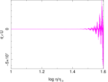
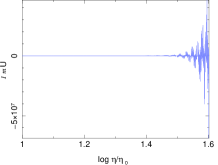
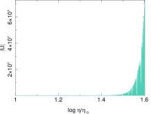
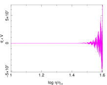
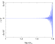
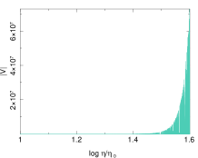
Figure 11: Real, imaginary, and absolute value of $U_{k}$ and $V_{k}$ for $\alpha=0$ and $\beta=100$. The general aspects of these functions are not very sensitive to $\alpha$ and are very similar for $\beta\gtrsim 10$. Note that although there are resonant jumps in the value of $U$ and $V$, due to complicated interaction terms they are not regular as in the preheating.

4.4.3 Backreaction

An exponential growth of the condensate for ever would be evidently catastrophic for this model. We show below that during matter domination era the faster expansion of the Universe stops the growth. Moreover, if $X$ particles have a short lifetime and decay completely before the end of the radiation domination epoch, production term in (41) becomes negligibly small. Due to many simplifying assumptions we had to make to be able to obtain approximative analytical solutions (70) and (70), some other issues must be also taken into account. For instance, we neglected the effect of free $\phi$ particles. Energy transfer between them and the condensate can lead to evaporation of the latter. This effect would be consistently taken into account if we solve Boltzmann/Kadanoff-Baym equations along with evolution equation of the condensate and add 2PI terms in the evolution of propagators.

4.4.4 Matter domination era

In the matter domination epoch the relation between comoving and conformal time deviates from the previous era and consequently the evolution equation of fields is different and has the following form:

$$\mathcal{U}_{k}^{\prime\prime}+(k^{2}+\frac{m^{2}a_{0}^{2}\eta^{4}}{\eta_{0}^{4}}-\frac{2}{\eta^{2}})\mathcal{U}_{k}=0$$ (72)

In contrast to radiation domination epoch, this equation does not have known analytical solution. Only for two special cases of $m=0$ and $k^{2}=0$ exact analytical solutions exist. Therefore, we have to use one of them, in preference the solution of $k^{2}=0$ which is closer to the case we are interested in, along with WKB approximation. When interactions are ignored the solution of the evolution equation has the following approximate expression:

$$\chi_{k}(\eta) \xrightarrow[\lambda=0]{\frac{\eta}{\eta_{0}}\gg 1} \sqrt{\frac{2}{\pi\beta^{\prime}_{\Phi}}}\frac{\eta_{0}}{\eta}\biggl{(}1-\frac{3k^{2}\eta_{0}}{2m_{\Phi}^{2}\eta}+\mathcal{Y}_{k}(\eta)\biggr{)}\biggl{\{}{c^{\prime}}_{k}^{(a)}\sin\biggl{(}\beta^{\prime}\frac{\eta^{3}}{\eta_{0}^{3}}(1-\frac{3k^{2}\eta_{0}}{2m_{\Phi}^{2}\eta})+\mathcal{Y}_{k}(\eta)\biggr{)}+$$ (73)

$${d^{\prime}}_{k}^{(a)}\cos\biggl{(}\beta^{\prime}\frac{\eta^{3}}{\eta_{0}^{3}}(1-\frac{3k^{2}\eta_{0}}{2m_{\Phi}^{2}\eta})+\mathcal{Y}_{k}(\eta)\biggr{)}\biggr{\}}$$

$$\mathcal{Y}_{k}(\eta) = \frac{i\mathsf{g}^{2}}{4(2\pi)^{3}\pi\sqrt{\beta^{\prime}_{A}\beta^{\prime}_{X}}}\biggl{\{}\sum_{\alpha}C_{\alpha}(k,\bar{x})\gamma(-2,i\alpha\frac{\eta^{3}}{\eta_{0}^{3}})+$$ (74)

$$\sum_{\alpha}C^{\prime}_{\alpha}(k,\bar{x})\gamma(-\frac{1}{3},i\alpha\frac{\eta^{3}}{\eta_{0}^{3}})\biggr{\}}$$

where $C_{\alpha}$ and $C^{\prime}_{\alpha}$ are proportional to the distributions of $A$ and $X$ particles and $\beta^{\prime}\equiv\frac{a_{0}\eta_{0}m}{3}=\frac{2m}{3H_{0}}$. At late times $\gamma$-functions in (74) approach a constant and $\bar{x}$ dependent terms i.e terms containing $f^{(A)}$ and $f^{(X)}$ decay very rapidly, as $(\eta_{0}/\eta)^{6}$ for terms containing one $f$, and $\chi_{k}(\eta)$ becomes an oscillating function that its amplitude decreases as $\eta_{0}/\eta$ with time. Consequently, $\varphi_{k}$ decreases as $\eta^{3}_{0}/\eta^{3}$ and the production of $\Phi$ in the decay of $X$ alone is not enough to compensate the expansion of the Universe, leading to a decreasing density of the condensate. Evidently, the validity of this conclusion depends on the precision of approximations considered in this calculation. In fact it is shown [20] that linearized equations always arrive to the same conclusion, even when all interactions are taken into account.

To perform a nonlinear analysis of the condensate equation with self-interaction we first neglect quantum corrections. This means that we only consider the classical interaction term in (37) for which the minimum of the potential is at origin. If for simplicity we neglect also the production term, the evolution equation becomes:

$${\chi}^{\prime\prime}+(k^{2}+a^{2}m_{\Phi}^{2}-\frac{2}{\eta^{2}})\chi+\lambda a^{4-n}\chi^{n-1}(x)=0$$ (75)

Using a difference approximation for derivatives but without linearization, we find that although at the beginning $\chi$ can grow irrespective of initial conditions, at late times it approaches zero. This means that this equation lacks a tracking solution. Another way of checking the absence of a tracking solution is the application of the criterion $\Gamma\equiv V"V/V^{\prime}2>1$ proved to be the necessary condition for the existence of such solutions [46]. For equation (75) $\Gamma=n(n-1)/n^{2}<1$ for $n>0$. This is a well known result. As mentioned in section 3, only inverse power-law and inverse exponential potentials have a late time tracking solution [41].

When quantum corrections are added, the evolution equation depends on the coefficient $C$ which appears in the expression of propagators and determines the amplitude of the quantum state of the condensate. This coefficient depends inversely on $\chi$, see (53), and thereby induces a backreaction from the formation of the condensate to the propagators of $\phi$ and vis-versa. After adding these non-linear terms to the evolution equation of the quintessence condensate, it has the following approximate expression:

$${\chi}^{\prime\prime}+(k^{2}+a^{2}m_{\Phi}^{2}-\frac{2}{\eta^{2}})\chi+\frac{i}{3}\lambda^{2}a^{4-n}(\frac{2}{\pi\beta^{\prime}_{\Phi}})^{n-2}e^{i\frac{(8-n)\pi}{6}}(\frac{\eta_{0}}{\eta})^{n-1}\sum_{\alpha,\beta}\beta^{-\frac{8-n}{3}}\gamma(\frac{8-n}{3},-i\beta\frac{\eta^{3}}{\eta_{0}^{3}})~{}e^{i(\alpha+\beta)\frac{\eta^{3}}{\eta_{0}^{3}}}$$

$$\quad\quad\times\sum_{i=1}^{n-1}\binom{n-1}{i}(\frac{2}{\pi\beta^{\prime}_{\Phi}})^{n-i}\cos^{2(n-i)}(\beta^{\prime}_{\Phi}\frac{\eta^{3}}{\eta_{0}^{3}})~{}(\frac{\eta_{0}}{\eta})^{2(n-i)}~{}\chi^{-2(n-i)+1}(\eta)+\ldots=0$$

$$\alpha,\beta=j\beta^{\prime}_{\Phi},\quad\quad j=-(n-1),\ldots,n-1$$ (76)

where dots indicates subdominant terms. The effective potential in this equation includes negative power terms which can satisfy tracking condition if they vary slowly with time. Using the asymptotic expression of incomplete $\gamma$-function and counting the order of $\eta/\eta_{0}$ terms, we conclude that terms satisfying the following conditions vary slowly for $\eta/\eta_{0}\gg 1$:

$$\alpha=-2\beta,\quad\quad 17-6n+2i\geqslant 0$$ (77)

The first condition eliminates the oscillatory terms, and the second one corresponds to orders of $\eta/\eta_{0}$ terms satisfying the tacking solution condition. As $i\leqslant n-1$, this condition is satisfied only for $n\leqslant 3$. The case of $n=4$ is also interesting, because although the indices of time-depending terms would be positive, the decay of the density of condensate would be enough slow such that its equation of state may be still consistent with observations. It is remarkable that these values for the self-interaction order are the only renormalizable polynomial potentials in 4-dimension spacetimes. The study of dark energy domination era is more complicated because the evolution equations of the condensate and expansion factor $a(\eta)$ become strongly coupled and must be solved numerically.

4.5 Outline

In [20, 92, 91], we used non-equilibrium quantum field theory techniques to study the condensation of a scalar field during cosmological time. The scalar was assumed to be produced by the decay of a much heavier particle. Similar processes had necessarily happened during the reheating of the Universe. They could have happened at later times too if the remnants of the decay did not significantly perturb primordial nucleosynthesis. To fulfill this condition the probability of such processes had to be very small. We showed that one of the necessary conditions for the formation of a condensate is its light mass and small self-interaction which have important roles in the cosmological evolution of the condensate and its contribution to dark energy. In particular, we showed that only a self-interaction of order $\lesssim 4$ can produce a stable condensate in matter domination epoch. Confirmation of these results and the extension of the analysis to dark energy domination epoch needs lattice numerical calculation which is a project for near future.

We conclude this section by reminding that if dark energy is the condensate of a scalar field, the importance of the quantum coherence in its formation and evolution would be the proof of the reign of Quantum Mechanics at largest observable scales of the Universe.

5 Parametrization and test of dark energy models

5.1 Introduction

Modeling a physical phenomenon would not be useful if we cannot distinguish between candidate models. Specially, in what concerns the origin of accelerating expansion of the Universe, since its observational confirmation in the second half of 1990’s, a large number of models are suggested to explain this phenomenon. In section 1 we briefly reviewed the most popular categories of dark energy models. However, when it comes to their observational verification, the difficulty of the task oblige us to be more general, and at this stage only target the discrimination between three main category of dark energy:

• Cosmological constant

• Quintessence

• Modified gravity

Fig. 12 shows these categories and their possible impacts on various observables which can be potentially used to pin down or constrain the underlying model and discriminate it from other dark energy candidates. In fact, a notable difference between a cosmological constant, modified gravity and some of quintessence models is the presence of a weak interaction between matter and dark energy in the last two cases which can potentially leave, in addition to its effects on the large scale distribution of matter, other distinguishable imprints such as a hot/warm dark matter. Prospectives for multi-probe studies of dark energy is discussed in the next chapter.

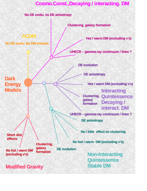
Figure 12: The major categories of dark energy models and observables that potentially carry their imprint. A simpler version of this diagram is published in [110]. Question marks mean that the effect is model dependent.

There are essentially two main cosmological observables which through their measurements cosmological parameters can be determined. The first observable is the expansion rate of the Universe - Hubble function $H(z)$ and its evolution with redshift. The second quantity is the distribution of matter anisotropies. The measurement of the first quantity needs a standard candle - an object with known luminosity or dimension. As for the second quantity, because most of matter in the Universe is dark, its distribution can only be measured indirectly through anisotropies that it induces in the distribution of Cosmic Microwave Background (CMB) and galaxies, or through its gravitational lensing effects. To be able to interpret measurements, specially for the purpose of discriminating among models, it is necessary to have quantitative descriptions for observables which can be universally applied to models irrespective of their details.

5.2 Nonparametric determination of dark energy evolution

Every content of the Universe has a contribution in the Friedmann equation that governs the evolution of expansion factor of the Universe:

$$H^{2}(z)=(\frac{\dot{a}}{a})^{2}(z)=\frac{8\pi G}{3}\sum_{i}\rho_{i}$$ (78)

Therefore, the measurement of the expansion rate - the Hubble function - and its evolution are the most direct means for understanding homogeneous properties of dark energy. In a fluid approximation various contents of the Universe are characterized and distinguished by their equation of state $w$ defined in (10). For a cosmological constant $w_{de}=-1$. This value can be considered as a critical point, because as we discussed in detail in section 3, models with $w<-1$ apriori break the null energy theorem of general relativity, and therefore negative $w+1$ must be either an effective value or related to an exotic phenomenon such as a nonstandard kinetic term. For this reason, it is more useful to measure the sign of $w+1$, i.e. the direction of its deviation from the critical point, rather than its exact value which is less crucial for discriminating between models and more prone to measurement errors. The purpose of the work reported in [111, 112, 110] was to find a suitable methodology to determine the sign of $w+1$ in a nonparametric manner. The expression nonparametric in signal processing literature means testing a null hypothesis against an alternative by using a discrete condition such as a jump or the change of a sign rather than constraining a continuous parameter (see e.g. [113]). Therefore, for determining the sign of $w+1$ we need to find a quantity proportional to it irrespective of uncertainties of other parameters, as long as they are limited to a reasonable range.

In a flat universe containing cold matter, radiation and dark energy, all approximated by fluids, the density at redshift $z$ can be written as:

$$\frac{\rho(z)}{\rho_{0}}=\Omega_{m}(1+z)^{3}+\Omega_{h}(1+z)^{4}+\Omega_{de}(1+z)^{3\gamma}$$ (79)

where $\rho(z)$ and $\rho_{0}$ are respectively the total density at redshift $z$ and at $z=0$, $\Omega_{m}$, $\Omega_{h}$, and $\Omega_{de}$ are respectively the fraction of cold matter, radiation, and dark energy in the total density at $z=0$. For a constant $w$ (i.e. when it does not depend on $z$), $\gamma=w+1$, and it can be easily shown that in this case:

$${\mathcal{A}}(z)\equiv\frac{1}{3(1+z)^{2}\rho_{0}}\frac{d\rho}{dz}-\Omega_{m}=\gamma\Omega_{de}(1+z)^{3(\gamma-1)}$$ (80)

When various constituents of the Universe interact with each others, equations of states depend on $z$ and Friedmann equation and ${\mathcal{A}}(z)$ can be parametrized as the followings [114]:

$$\frac{H^{2}}{H_{0}^{2}}=\frac{\rho_{c}(z)}{\rho_{c0}}=\sum_{i}\Omega_{i}{\mathcal{F}}_{i}(z)(1+z)^{3\gamma_{i}},\quad\quad i=\text{{\it m, b, h,k,} and {\it de}}$$ (81)

where $m=$ cold dark matter, $b=$ baryons, $h=$ hot matter (radiation), $k=$ curvature, and $de=$ dark energy.

$$\gamma(z)=\frac{1}{\ln(1+z)}\int_{0}^{z}dz^{\prime}\frac{1+w(z^{\prime})}{1+z^{\prime}}$$ (82)

$${\mathcal{B}}(z) \equiv \frac{1}{3(1+z)^{2}\rho_{0}}\frac{d\rho}{dz}=\frac{-(2\frac{dD_{A}}{dz}+(1+z)\frac{d^{2}D_{A}}{dz^{2}})}{\frac{2}{3(1+z)^{2}}(D_{A}+(1+z)\frac{dD_{A}}{dz})^{3}}$$ (83)

$$= \sum_{i=m,h,k}\Omega_{i}\biggl{(}\gamma_{i}{\mathcal{F}}_{i}(z)+(1+z)\frac{d{\mathcal{F}}_{i}}{dz}\biggr{)}(1+z)^{3(\gamma_{i}-1)}+\Omega_{de}(w(z)+1)(1+z)^{3(\gamma_{de}(z)-1)}$$

$${\mathcal{A}}(z) \equiv {\mathcal{B}}(z)-\sum_{i=m,h,k}\Omega_{i}\gamma_{i}(1+z)^{3(\gamma_{i}-1)}$$ (84)

$$= \sum_{i=m,h,k}\Omega_{i}\biggl{(}\gamma_{i}({\mathcal{F}}_{i}(z)-1)+(1+z)\frac{d{\mathcal{F}}_{i}}{dz}\biggr{)}(1+z)^{3(\gamma_{i}-1)}+\Omega_{de}(w(z)+1)(1+z)^{3(\gamma_{de}(z)-1)}$$

It is clear that the sign of ${\mathcal{A}}(z)$ follows the sign of $\gamma$. Moreover, giving the fact that according to observations $\gamma\approx 0$, the exponent of $z$-dependent term in the r.h.s. of (84) is always negative. This means that the maximum of ${\mathcal{A}}(z)$ is at $z\rightarrow 0$ where more precise data from standard candles such as supernovae type Ia are available. Another advantage of ${\mathcal{A}}(z)$ to direct determination of $\gamma$ from Friedmann equation is the fact that at low redshifts this equation is insensitive to the value of $\gamma$ [114]. In fact, using the definition of angular diameter distance $D_{A}(z)$, which in addition to supernovae data can be measured by Baryon Acoustic Oscillations (BAO), the Friedmann equation can be written as:

$$\ln\biggl{[}\biggl{(}\frac{d}{dz}((1+z)D_{A})\biggr{)}^{-1}-\Omega_{m}(1+z)^{3}-\Omega_{h}(1+z)^{4}-\Omega_{K}(1+z)^{2}\biggr{]}=\ln\Omega_{de}+3\gamma(z)\log(1+z)$$ (85)

At small redshifts the last term on the r.h.s. of (85) which contains $\gamma(z)$ approaches zero and its effect on the evolution of $D_{A}$ becomes negligibly small, irrespective of the value of $\gamma$.

When $dw/dz\ll 3w(z)(w(z)+1)/(1+z)$, the sign of $dA/dz$ is opposite to the sign of $w(z)+1$. This condition is satisfied at low redshifts - see examples of models in Fig. 13. Therefore, $A(z)$ is a concave or convex function of redshift, respectively for positive or negative $w(z)+1$. Observations show that the contribution of $\Omega_{k}$ and $\Omega_{h}$ at low redshifts are much smaller than the uncertainty of $\Omega_{m}$. The function $dA/dz$ does not depend on $\Omega_{m}$. Thus, the uncertainty on the value of $\Omega_{m}$ can shift the value of $A(z)$ but it does not change its slope and its shape i.e. its concavity or convexity that determines the sign of $\gamma$ is preserved. Moreover, the uncertainty of $H_{0}$ scales ${\mathcal{B}}(z)$ uniformly at all redshifts and does not change geometrical properties of ${\mathcal{A}}(z)$. In conclusion, in what concerns the determination of the sign of $w+1$, the functions ${\mathcal{A}}(z)$ and ${\mathcal{B}}(z)$ are less sensitive to uncertainties of cosmological parameters than $H(z)$ and $D_{A}(z)$.

Fig. 13 shows ${\mathcal{A}}(z)$ for several phenomenological models of dark energy and parametrizations of $w(z)$. It is clear that for given values of ${\mathcal{A}}(z)$ (or similar quantities) at two redshifts the conclusion about evolution of dark energy and thereby the underlying model depends on the parametrization. Therefore, it is preferable to extract $w(z)$ in a nonparametric manner from data which is described in detail in [114].

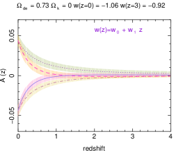
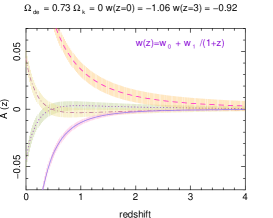
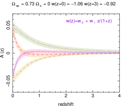
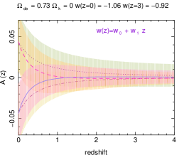
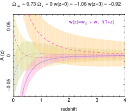
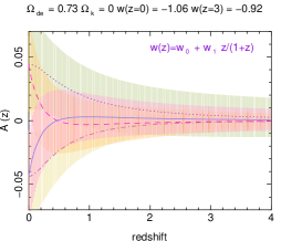
Figure 13: ${\mathcal{A}}(z)$ as a function of redshift. To see how well ${\mathcal{A}}(z)$ can distinguish between various models and how systematic and statistical errors and parametrization affect the reconstructed model, we consider 3 parametrizations as written on the plots above. Note that parametrizations for the plot in the center and on the right are equivalent up to a redefinition of coefficients $w_{0}$ and $w_{1}$. All the examples have the same value of $w(z)$ at $z=0$ and $z=3$. After determining the corresponding coefficients $w_{0i}$ and $w_{1i}$ where index $i$ means initial. Then, to simulate systematic errors we have plotted the following models: $w_{0}=-1+|w_{0i}+1|$, $w_{1}=w_{1i}$ (dot), $w_{0}=-1-|w_{0i}+1|$, $w_{1}=-w_{1i}$ (dot-dash), $w_{0}=-1+|w_{0i}+1|$, $w_{1}=-w_{1i}$ (dash) and $w_{0}=w_{0i}$ and $w_{1}=w_{1i}$ (full). Colored vertical bars present statistical errors. The uncertainty of ${\mathcal{A}}(z)$ is $1\sigma_{{\mathcal{A}}(z=0)}=0.01$ (top row) and $1\sigma_{{\mathcal{A}}(z=0)}=0.05$ (bottom row) at $z=0$ and evolves with redshift as $\sigma_{\mathcal{A}}(z)=\sigma_{\mathcal{A}}(z=0)(1+z)^{2}$. It seems to be possible to distinguish between normal and phantom dark energy models easily if uncertainties are limited to few percents. Evidently, achieving such a precision is challenging even for space missions such as Euclid.

5.2.1 Error estimation for nonparametric sign detection

Fig. 14 shows the comparison of ${\mathcal{A}}(z)$ calculated from supernovae data with dark energy models having positive and negative $w+1$. Visual inspection clearly concludes that both data-sets shown in this figure are consistent with $w+1\lesssim 0$ in the interval $z\lesssim 0.5$. However, visual inspections or even the measurement of the slope lacks a quantitative estimation of uncertainties. In signal processing a binomial estimation of the probability or optimization of detection [115] are usually used to assess uncertainties. In fact, in most practically interesting contexts in signal processing the signal is constant and uncertainties are due to the noise. In the cosmological case discussed here the observable ${\mathcal{A}}(z)$ is both noisy and varies with redshift. Therefore, binomial probability and similar methods are not suitable. For this reason in [111] another strategy which is specially appropriate for cosmological quantities is proposed.

The null hypothesis for dark energy is $\gamma=0$, i.e. $\Lambda$CDM. Assuming a Gaussian distribution for the uncertainties of the reconstructed ${\mathcal{A}}(z)$ from data and from simulated data with $\gamma=0$, for each data-point we calculate the probability that it belongs to the null hypothesis. To include the uncertainty of data, we integrate the uncertainty distribution 1-sigma around its mean value:

$$P_{i}=\frac{1}{\sqrt{2\pi(\sigma_{0i}^{2}+\sigma_{i}^{2})}}\int_{{\mathcal{A}}_{i}-\sigma_{i}}^{{\mathcal{A}}_{i}+\sigma_{i}}dxe^{-\frac{(x-{\mathcal{A}}_{0i})^{2}}{2(\sigma_{0i}^{2}+\sigma_{i}^{2})}}$$ (86)

where ${\mathcal{A}}_{i}$ and $\sigma_{i}$ belong to the $i^{th}$ data-point, and ${\mathcal{A}}^{0i}$ and $\sigma_{0i}$ belong to the simulated null hypothesis model at the same redshift. Averaging over $P_{i}$ gives $\bar{P}$, an overall probability that the dataset corresponds to the null hypothesis. As $\gamma=0$ is the limit case for $\gamma>0$, $\bar{P}$ is also the maximum probability of $\gamma>0$.

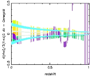
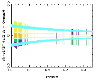
Figure 14: Left: ${\mathcal{A}}(z)$ from 117 supernovae from the SNLS survey (purple). Error bars are 1-sigma uncertainty. Green, orange, yellow, and light green curves are the reconstruction of ${\mathcal{A}}(z)$ from simulations for $\gamma=-0.2,-0.06,0.6,0.2$, respectively. The probability of null hypothesis ($\gamma=0$) is $\bar{P}=0.27$, therefore the probability of $\gamma<0$, $1-\bar{P}=0.73$. Light grey and cyan curves are theoretical calculation including the uncertainty on $\Omega_{de}$, respectively for $\gamma=\pm 0.06,\pm 0.2$. For all models $H_{0}=73~{}km~{}Mpc^{-1}~{}sec^{-1}$ and $\Omega_{de}=0.77$ and $5\%$ errors for each. Right: ${\mathcal{A}}(z)$ for SNLS supernovae with $z<0.45$. Definition of curves and cosmological parameters are the same as the left plot. For this dataset $1-\bar{P}=0.93$. If $\Omega_{de}=0.73$ is used, $1-\bar{P}=0.96$.

5.2.2 Precision of model discrimination

Using generalized parametrization of Friedmann equation (81), in [114] it is shown, with explicit examples, that discrimination between modified gravity and some categories of quintessence models is possible. Notably, if data is analyzed with the null hypothesis of no interaction, when in reality there is an interaction in the dark sector, the effective values of $\Omega_{de}$ and $\gamma_{de}$ extracted from measurements of the Hubble function $H(z)$ and from ${\mathcal{A}}$ will not be the same. Therefore, for detecting the tiny signature of an interaction in the dark sector, rather than fitting the data with a large number of parameters, it is better to measure the difference between two pair of measurements $(\Omega_{eff}^{(H)},~{}\gamma_{eff}^{(H)})$ and $(\Omega_{eff}^{(A)},~{}\gamma_{eff}^{(A)})$. For this purpose, a natural criterion is:

$$\Theta(z)\equiv\frac{\Omega_{eff}^{(A)}(w_{eff}^{(A)}(z)+1)(1+z)^{3\gamma_{eff}^{(A)}(z)}-\Omega_{eff}^{(H)}(w_{eff}^{(H)}(z)+1)(1+z)^{3\gamma_{eff}^{(H)}(z)}}{\Omega_{eff}^{(H)}(w_{eff}^{(H)}(z)+1)(1+z)^{3\gamma_{eff}^{(H)}(z)}}$$ (87)

This quantity can be explained explicitly as a function of $\Omega_{i},~{}{\mathcal{F}}_{i},~{}$ and $\gamma_{i}$, for $i\in{m,~{}h,~{}k,~{}de}$. The variable $\Theta(z)$ is zero when $F_{i}=1,~{}dF_{i}/dz=0$. In addition, this expression can be used to determine the absolute sensitivity of a survey on an interaction in the dark sector, irrespective of the measured proxy and data analyzing methods. We should also remark that many authors have used quantities similar to ${\mathcal{A}}(z)$ that depend on the evolution of Hubble function $dH/dz$, see e.g. [116]. Nonetheless, the work presented in [111, 112] is unique in proposing a nonparametric data analysing method for discriminating between dark energy models.

Assuming that $\Omega_{m}$ and $\Omega_{h}$ can be determined independently and with very good precision, for instance from CMB anisotropies with marginalization over $\gamma_{de}$, the quantity $\Theta$ may be determined from the measurement of $H(z)$ and ${\mathcal{B}}(z)$ by using data from whole sky or wide area spectroscopic surveys such as Euclid, or multi-band photometric surveys such as DES.

5.3 Using LSS data for discriminating between dark energy models

Fig. 12 indicates that the deviation of matter clustering and spectrum of perturbations from predictions of $\Lambda$CDM are definitive signatures of interaction in the dark sector. Thus, along with the evolution of expansion rate discussed in the previous section, we must use LSS data to discriminate these models from $\Lambda$CDM and non-interacting quintessence. However, discrimination between modified gravity and interacting quintessence which both can be written as a scalar field model is not straightforward and more criteria are necessary. For this reason, in [114] along with the studies reviewed in the previous section, we have investigated properties and differences of interacting quintessence and modified gravity to find new criteria for discrimination between them. Moreover, we suggest a new parametrization of observables for this purpose.

5.3.1 Discrimination according to interaction type

By definition, in modified gravity it is expected that when it is written in Einstein frame, the scalar field has the same coupling to all species. However, as explained earlier this criterion is not suitable for observational and data analysing purposes, thus here we propose another criterion. But before explaining it, we review phenomenological description of interactions without a detail knowledge about the micro-physics of the underlying model.

In presence of non-gravitational interactions between constituents the energy-momentum tensor of each component $T^{\mu\nu}_{i}$ is not separately conserved, and conservation equations can be only written for the total energy-momentum tensor $T^{\mu\nu}$ defined as:

$$T^{\mu\nu}\equiv\sum_{i}T^{\mu\nu}_{i(free)}+T^{\mu\nu}_{int}$$ (88)

$$T^{\mu\nu}_{;\nu}=\sum_{i}T^{\mu\nu}_{i(free)~{};\nu}+T^{\mu\nu}_{int~{};\nu}=0$$ (89)

where $T^{\mu\nu}_{i(free)}$ is the energy-momentum tensor of component $i$ in absence of interaction with other components. This means that $T^{\mu\nu}_{i(free);\nu}=0$ only if the free value of fields and dynamical variables are used in this conservation equation. In this case $\sum_{i}T^{\mu\nu}_{i(int)~{};\nu}=0$. In perturbative field theories, specially when one studies the scattering of particles, it is assumed that in the out-of-interaction region particles are free and this formalism are applicable. But, in cosmology there is no asymptotic freedom because we live inside the interaction region. In the literature on interacting dark energy models (see e.g. [50, 51]) when only two constituents - matter and dark energy - are considered, the energy-momentum conservation equations are usually written as:

$$T^{\mu\nu}_{m~{};\nu}=Q^{\mu},\quad T^{\mu\nu}_{\varphi~{};\nu}=-Q^{\mu}$$ (90)

for an arbitrary interaction current $Q^{\mu}$. By comparing (89) and with (90), it becomes clear that tensors in the left hand side of equations in (90) do not correspond to free energy-momentum tensors, and along with $Q^{\mu}$ they are obtained somehow arbitrarily by division of (89). In fact, equations in (90) are inspired by perturbation theory in which for each perturbative order, the right hand sides of these equations are estimated using quantities from one perturbative order lower. Thus, they constitute an iterative set of equations from zero order (free) model in which $Q^{\mu}=0$, up to higher orders. This approach is not suitable for dark energy where we ignore, not only interactions but also the free model. Therefore, in place of (90) we use the following general expression:

$$T^{\mu\nu}_{m~{};\nu}=-Q_{m}^{\mu},\quad T^{\mu\nu}_{\varphi~{};\nu}=-Q_{\varphi}^{\mu},\quad T^{\mu\nu}_{int~{};\nu}=Q_{m}^{\mu}+Q_{\varphi}^{\mu}$$ (91)

In these equations matter and dark energy tensors $T^{\mu\nu}_{m}$ and $T^{\mu\nu}_{\varphi}$ have the same expression as in the absence of interaction, but with respect to fields which are not free (dressed fields). These expressions can be justified by considering the effective Lagrangian. In Einstein frame the Lagrangian for a weakly interacting system can be divided to free and interaction parts:

$${\mathcal{L}}=\sum_{i}{\mathcal{L}}_{i}+{\mathcal{L}}_{int}$$ (92)

Considering only local interactions, in the dynamics equations of fields the partial derivative of ${\mathcal{L}}_{int}$ with respect to each field determines the interaction term. Dynamics equations can be related to energy-momentum conservation equations (90) [16]. Therefore, interaction currents $Q_{m}^{\mu}$ and $Q_{\varphi}^{\mu}$ are generated by partial derivatives of ${\mathcal{L}}_{int}$ with respect to the corresponding interacting fields.

The scalar field in scalar-tensor modified gravity models is related to a dilaton. Consequently, the interaction term in these models is proportional to the trace of matter because it appears in the Lagrangian along with the metric. In this case, there is no interaction between the scalar field and relativistic particles, and it can be shown that $Q_{m}^{\mu}=-Q_{\varphi}^{\mu}$ [117] and $T^{\mu\nu}_{int~{};\nu}=0$. The interaction current $Q^{\mu}$ for these models can be written as:

$$Q^{\mu}={\mathcal{C}}(\varphi)T_{m}\partial^{\mu}\varphi$$ (93)

where $T_{m}=g_{\mu\nu}T^{\mu\nu}_{m}$ is the trace of the energy-momentum tensor. In the literature interaction current of interacting dark energy models is usually considered to be like in (93). Therefore, we classify models with this type of interaction as modified gravity. In interacting quintessence models the interaction can be more diverse, notably it may depend on matter species. Below we present a phenomenological description for them without considering details of the underlying model.

In quantum field theory, interactions can be easily included in the Lagrangian of the model. But this approach is usually useful if the microphysics of the model is studied. To be able to compare models with data, in observational cosmology we need macroscopic descriptions. For this reason, one usually uses fluid descriptions for fields. The transformation of the Lagrangian written with respect to fields to a fluid description is straightforward and energy-momentum tensor of interactions can be also described in fluid form without any ambiguity. However, their descriptions as a function of density and pressure of fluids depend on the details of interactions. For instance, a Higgs-like interaction between a scalar and a fermion $\propto\varphi\bar{\psi}\psi$ is described as $\propto(\rho_{\psi}-P_{\psi})(\rho_{\varphi}-P_{\varphi})^{1/2}$ if the self-coupling potential $V(\varphi)\propto\varphi^{2}$, and as $\propto(\rho_{\psi}-P_{\psi})(\rho_{\varphi}-P_{\varphi})^{1/4}$ if $V(\varphi)\propto\varphi^{4}$. Therefore, when the objective is a general parametrization of interactions without considering details of the underlying model, this type of description is not very suitable.

A macroscopic description of the Lagrangian alone is not sufficient for describing microscopic processes which need the Boltzmann equation. In fact, it is well known that Boltzmann equation plays the role of the intermediate between quantum and classical description of interacting systems. Species are described by their phase space distribution $f(p,x)$ where $p$ and $x$ are respectively momentum and spacetime coordinates. Interactions are included in the equation as collisional terms, and one can obtain energy-momentum and number conservation equations directly by using properties of the Boltzmann operator, see e.g. [118]. In the context of interacting dark energy models, the simplest examples of collisional terms are elastic scattering between dark matter and dark energy, and slowly decay of dark matter with a small branching ratio to dark energy similar to the model explained in section 3. Finally, after some simplifying approximations, we find following expressions for the interaction terms of dark energy and dark matter component:

$$T^{\mu\nu}_{m~{};\nu}\approx-\Gamma_{m}n_{m}^{\mu}+A_{ms}n_{m}^{\mu}u_{\varphi\rho}n_{\varphi}^{\rho}\equiv Q_{m}^{\mu}$$ (94)

$$T^{\mu\nu}_{\varphi~{};\nu}\approx\Gamma_{\varphi}n_{m}^{\mu}+A_{\varphi s}n_{\varphi}^{\mu}u_{m\rho}n_{m}^{\rho}\equiv Q_{\varphi}^{\mu}$$ (95)

where constants $\Gamma_{i}$ and $A_{is}$ are decay width and scattering amplitude for species $i$. In the rest of this section we use these equations as an approximation for energy-momentum conservation equations irrespective of dark matter type (its spin) and details of interaction between two dark components. These details affect constants $\Gamma_{i}$ and $A_{is}$ which are used as parameters. One can also add dark matter self-annihilation term to (94). But, as it is proportional to $|n_{m}|^{2}$ its effect is significant only in dense regions and small spatial scales such as the central region of dark matter halos which are in nonlinear regime and were not studied in [114].

5.4 Parameters of background cosmology in interacting models

Now that we have interaction terms for the two main classes of interacting dark energy models we can determine ${\mathcal{F}}_{i}$ parameters defined in (81).

• Modified gravity Using the energy momentum conservation equation (91) and the interaction current for modified gravity models, the scalar field equation and the evolution equation of the homogeneous matter density are determined [117]:

  $$\bar{\varphi}^{\prime\prime}+2{\mathcal{H}}\bar{\varphi}^{\prime}+a^{2}V_{\varphi}(\bar{\varphi})=a^{2}{\mathcal{C}}(\bar{\varphi})\sum_{i}(\bar{\rho}_{i}-3\bar{P}_{i}),\quad{\mathcal{H}}=\frac{a^{\prime}}{a}$$ (96)

  $$\bar{\rho}^{\prime}_{i}+3{\mathcal{H}}(\bar{\rho}_{i}+\bar{P}_{i})={\mathcal{C}}(\bar{\varphi})\bar{\varphi}^{\prime}(\bar{\rho}_{i}-3\bar{P}_{i})\quad i=m,~{}b,~{}h$$ (97)

  where barred quantities are homogeneous components and $\varphi$ in subscript means derivative with respect to $\varphi$. Note that here we have generalized the original calculation in [117] by considering a $\varphi$-dependent ${\mathcal{C}}(\bar{\varphi})$ coefficient in the right hand side of these equations rather than the constant value of models ${\mathcal{C}}=\sqrt{4\pi G/3}$ for $\mathrm{f}(R)$ models [117]. Equations (96) and (97) are coupled and an analytical solution cannot be found without considering an explicitly $V(\varphi)$. Therefore, to solve the equation for $\bar{\rho}$, which is in fact the only directly observable quantity, we simply consider the right hand side of the equation as a time-dependent source. The solution of equation (97) can be written as:

  $$\bar{\rho}_{i}(z)=\bar{\rho}_{i}(z_{0})(1+z)^{3(1+w_{i})}e^{(1-3w_{i})F(\bar{\varphi})},\quad F(\varphi)\equiv\int{\mathcal{C}}(\bar{\varphi})d\varphi,\quad i=m,b,h$$ (98)

  where $w_{i}\equiv\bar{P}_{i}/\bar{\rho}_{i}$ for all species except dark energy are assumed to be constant. Comparing this solution with (81) we find:

  $${\mathcal{F}}_{i}(z)=e^{(1-3w_{i})F(\bar{\varphi}(z))}\approx 1+(1-3w_{i})F(\bar{\varphi}(z))$$ (99)

• Interacting quintessence In the same way, we can determine ${\mathcal{F}}_{i}$ coefficients for (interacting)-quintessence using equation (94). After taking some approximations discussed in detail in [114], the evolution equation of densities in interacting quintessence models becomes:

  $$\bar{\rho}^{\prime}_{i}+3{\mathcal{H}}(\bar{\rho}_{i}+\bar{P}_{i})=-\Gamma_{i}a\bar{\rho}_{i}+A_{si}a\bar{\rho}_{i}\bar{\rho}_{\varphi}$$ (100)

  where $i$ indicates any cold matter or relativistic species that interact with quintessence field. A clear difference between interaction term in (100) and (97) is that the former does not explicitly depend on the scalar field, and therefore we do not need to know and solve a field equation similar to (96). The solution of this equation and corresponding ${\mathcal{F}}_{i}$’s are:

  $$\bar{\rho}_{i}(z) = \bar{\rho}_{i}(z_{0})(1+z)^{3(1+w_{i})}\exp\biggl{(}\Gamma_{i}(\tau(z)-\tau(z0))+A_{si}\int dz\frac{\bar{\rho}_{\varphi}(z)}{(1+z)H(z)}\biggr{)}$$ (101)

  $${\mathcal{F}}_{i}(z) = \exp\biggl{(}-\Gamma_{i}(\tau(z)-\tau(z_{0}))+A_{si}\int dz\frac{\bar{\rho}_{\varphi}(z)}{(1+z)H(z)}\biggr{)}\approx 1+\Gamma_{i}(\tau(z_{0})-\tau(z))+$$ (102)

  $$A_{si}\int_{z_{0}}^{z}dz\frac{\bar{\rho}_{\varphi}(z)}{(1+z)H(z)}$$

  where $\tau(z)$ is the age of the Universe at redshift $z$. Note that even in absence of expansion, the density of dark matter at high redshifts (large distances from us) is higher if $\Gamma_{m}>0$.

Along with consistency relation explained above for modified gravity models, explicit dependence of (102) on measurable quantities $\bar{\rho}_{\varphi}(z)$ and $H(z)$ apriori allows to discriminate between interacting quintessence and modified gravity models. However, the prior knowledge about the evolution of these quantities are mandatory for distinguishing the underlying model and without such information one cannot single out any model.

5.5 New parametrization of perturbations in interacting dark energy models

The criteria proposed in this section for distinguishing between modified gravity and interacting quintessence models are based on their interactions. Therefore, we expect different evolution for matter anisotropies and dark energy density in these models. In fact, if we could decompose the interaction current to terms proportional to scalar metric perturbations and matter density fluctuations, it were possible to distinguish between models easily. However, in practice measured quantities are the power spectrum of matter perturbations and its growth rate $\mathbf{f}(z,k)$ defined as:

$$\mathbf{f}(z,k)\equiv\frac{d\ln D}{d\ln a}=\frac{\delta^{\prime}_{m}}{{\mathcal{H}}\delta_{m}},\quad D\equiv\frac{\delta_{m}(z,k)}{\delta_{m}(z=0,k)}$$ (103)

The function $\mathbf{f}(z,k)$ is usually extracted from the power spectrum using a model [119], for instance a power-law for the primordial spectrum, modified to include Kaiser effect and redshift distortions due to the velocity dispersion.

To obtain the evolution equation of $\mathbf{f}(z,k)$, we replace gravitational potentials $\psi$ and $\phi$ by expressions depending only on $\delta_{m}\equiv\delta\rho_{m}/\bar{\rho}_{m}$ and $\theta_{m}\equiv ik_{j}v_{(m)}^{j}$. Assuming a negligible anisotropic shear at $z\lesssim\mathcal{O}(1)$ which concerns galaxy surveys, scalar metric perturbations $\psi$ and $\phi$ can be determined from Einstein equations:

$$ds^{2} = a^{2}(\eta)\biggl{[}(1+2\psi)d\eta^{2}-(1-2\phi)\delta_{ij}dx^{i}dx^{j}\biggr{]}$$ (104)

$$\phi=\psi = \frac{4\pi G\bar{\rho}_{m}}{k^{2}}\bigg{(}\delta_{m}+3(1+w_{m})\frac{{\mathcal{H}}\theta_{m}}{k^{2}}\biggr{)}+\Delta\psi$$ (105)

$$\phi^{\prime} = -\frac{4\pi G\bar{\rho}_{m}{\mathcal{H}}}{k^{2}}\biggl{(}\delta_{m}+(3+\frac{k^{2}}{{\mathcal{H}}^{2}})(1+w_{m})\frac{{\mathcal{H}}\theta_{m}}{k^{2}}\biggr{)}+\Delta\phi^{\prime}$$ (106)

In (105) and (106) terms that vanish for $\Lambda$CDM model are included in $\Delta\psi$ and $\Delta\phi^{\prime}$. They can be described as a function of two new quantities $\epsilon_{0}$ and $\epsilon_{1}$:

$$\epsilon_{0}\equiv\frac{\delta\rho_{\varphi}}{\bar{\rho}_{m}},\quad\epsilon_{1}\equiv\frac{{\mathcal{H}}(\bar{\rho}_{\varphi}+\bar{P}_{\varphi})^{\frac{1}{2}}\delta\varphi}{\bar{\rho}_{m}}$$ (108)

$$\Delta\psi=\frac{4\pi G\bar{\rho}_{m}}{k^{2}}(\epsilon_{0}-3\epsilon_{1}),\quad\quad\Delta\phi^{\prime}=-\frac{4\pi G\bar{\rho}_{m}{\mathcal{H}}}{k^{2}}\biggl{(}\epsilon_{0}-(3+\frac{k^{2}}{{\mathcal{H}}^{2}})\epsilon_{1}\biggr{)}$$ (109)

After replacing $\phi^{\prime}$ and $\psi$ in the evolution equation of matter and velocity perturbations we can determine the evolution of growth rate which can be directly measured from galaxy distribution:

$$\mathbf{f}^{\prime}{\mathcal{H}}+\mathbf{f}({\mathcal{H}}^{\prime}+{\mathcal{H}}^{2})+\mathbf{f}^{2}{\mathcal{H}}^{2}+3(C_{sm}^{2}-w_{m})({\mathcal{H}}^{\prime}+\mathbf{f}{\mathcal{H}}^{2})+3(C_{sm}^{2}-w_{m}){\mathcal{H}}^{2}+$$

$$\quad\quad\quad\frac{3}{2}~{}\Omega_{m}(1+w_{m})^{2}{\mathcal{H}}^{2}+k^{2}C_{sm}^{2}+E_{0}\mathbf{f}{\mathcal{H}}+E_{1}k^{2}+E_{2}{\mathcal{H}}+E_{3}{\mathcal{H}}^{2}+E_{4}=0$$ (110)

Coefficients $E_{0},~{}E_{1},~{}E_{2},~{}E_{3},~{}E_{4}$ depend on $z$, $k$, equation of state of matter, sound speed, and parameters related to the interaction in the dark sector. The details of their expression can be found in [114]. For $\Lambda$CDM model $E_{i}=0,~{}i=0,\cdots,4$. For a non-interacting quintessence model all $E_{i}$ coefficients are zero except $E_{3}$. A notable difference between modified gravity and interacting quintessence models is the coefficient $E_{1}$ which is strictly zero for interacting dark energy models and nonzero for modified gravity which leaves an additional scale dependent signature on the evolution of matter anisotropies. The other explicitly scale dependent term is common among all models and is expected to be very small because it is proportional to the square of sound speed which is very small for cold matter. In addition, in contrast to other $E_{i}$ coefficients, $E_{1}$ and $E_{3}$ are dimensionless. Evidently, the contribution of $E_{1}k^{2}$ term in equation (110) with respect to other terms increases with $k$, i.e. at shorter distances. But, nonlinearity effects such as mode coupling also increase at large $k$. They can imitate an interaction in the dark sector and lead to misinterpretation of data. For this reason, simulations show that observations of galaxy clusters is a good discriminator between dark energy models [120], because they are still close to linear regime, but have relatively large $k$.

Discriminating quality of a survey can be estimated by the precision of $E_{1}$ and $E_{3}$ measurements. However, one expects some degeneracies when equation (110) is fitted to determine $E_{i}$’s. Moreover, in galaxy surveys, $\mathbf{f}$ and $\mathbf{f}^{\prime}$ (or more precisely $d\mathbf{f}/dz$) are determined from the measurement of the power spectrum, itself determined from the galaxy distribution, and ${\mathcal{H}}$ and ${\mathcal{H}}^{\prime}$ are determined from the BAO feature of the spectrum. Thus, these measurements are not completely independent. An independent measurement of ${\mathcal{H}}$ and ${\mathcal{H}}^{\prime}$ e.g. using supernovae will help to reduce degeneracies and error propagation from measured quantities to the estimation of $E_{i}$’s. The relation between ${\mathcal{H}}^{\prime}$ and $B(z)$ shows the logical connection between the parametrization of background cosmology and the evolution of fluctuations, specially in what concerns discrimination between dark energy models. In fact, anisotropies depend on the equation of state of matter, which in the framework of interacting dark energy models, is modified by its interaction with dark energy. Thus, their independent measurements optimize their employment in the procedure of distinguishing among various models.

5.6 Interpretation and comparison with other parametrizations

Definition of parameters $\epsilon_{0}$ and $\epsilon_{1}$ in (108) show that the former depends only on dark energy density anisotropies and the latter only on the peculiar velocity of dark energy field, i.e. on its kinematics. They follow each other closely and approach zero when the field approaches its minimum value. However, their exponent close to the minimum depends on the interaction. Therefore, their measurements give us information about the potential and interactions of the scalar field. Moreover, the difference in the dependence of the evolution equation of anisotropies and growth factor to these parameters shows that only by separation of kinematics and dynamics of dark energy it would be possible to distinguish between modified gravity and other scalar field models.

The deviation of gravity potentials $\phi$ and $\psi$ from their value in $\Lambda$CDM $\Delta\psi$ is the quantity which can be measured directly from gravitational lensing data. For this reason, various authors have used $\Delta\psi$ to parametrize the deviation of models and data from $\Lambda$CDM [121]. However, equations (105) and (109) show that although $\Delta\psi\neq 0$ is by definition a signature of deviation from $\Lambda$CDM, in contrast to claims in the literature, it is not necessarily the signature of a modified gravity because quintessence models, both interacting and non-interacting, also induce $\Delta\psi\neq 0$.

Because we have used Einstein frame for both quintessence and modified gravity models, in absence of an anisotropic shear $\phi=\psi$ even in models other than $\Lambda$CDM. At linear order, gravitational lensing effect depends on the total potential $\Phi\equiv\phi+\psi$. Therefore, in Einstein frame:

$$\Phi=2\phi=2\psi=\Phi_{\Lambda\text{CDM}}+2\Delta\psi,\quad\quad\Phi_{\Lambda\text{CDM}}\equiv\frac{4\pi G\bar{\rho}_{m}}{k^{2}}\bigg{(}\delta_{m}+3(1+w_{m})\frac{{\mathcal{H}}\theta_{m}}{k^{2}}\biggr{)}\equiv\frac{4\pi G\bar{\rho}_{m}}{k^{2}\Delta_{m}}$$ (111)

In the notation of [121] $\Phi=2\Sigma\Phi_{\Lambda\text{CDM}}$, thus:

$$\Sigma=1+\frac{\Delta\psi}{\Phi_{\Lambda\text{CDM}}}=\frac{\epsilon_{0}-3\epsilon_{1}}{k^{2}\Delta_{m}}$$ (112)

The other quantity which affects the evolution of lensing and directly depends on the cosmology is the growth factor of matter anisotropies which determines the evolution of $\Delta_{m}$ defined in (111). This quantity can be obtained from integration of growth rate $\mathbf{f}$ defined in (103) and is usually parametrized as $\Omega_{m}^{\gamma}$. For $\Lambda$CDM $\gamma\approx 0.55$ [122]. In this respect there is no difference between our formulation and what is used in the literature.

Our parametrization can be related to parameters $\eta$ and $Q$ used in the literature [121]: $\eta\equiv(\psi-\phi)/\phi$ and $Q=\phi/\phi_{\Lambda\text{CDM}}$. Thus, parameters $\Sigma$ and $\eta$ are not independent and $\Sigma=Q(1+\eta/2)$. In Einstein frame $\eta=0$ unless there is an anisotropic shear. At first sight it seems that there is less information in Einstein frame about modified gravity than in Jordan frame. However, one should notice that in Einstein frame the fundamental parameters are $\epsilon_{0}$ and $\epsilon_{1}$ and other quantities such as $\Delta\psi$ and $\mathbf{f}$ can be expressed with respect to them. Therefore, the amount of information in Einstein and Jordan frames about modified gravity is the same. The advantage of the formulation in Einstein frame and parameters $\epsilon_{0}$ and $\epsilon_{1}$ is that they can be used for both quintessence and modified gravity. Moreover, they have explicit physical interpretations that can be easily related to the underlying model of dark energy. Comparison of our parametrization with few others proposed recently can be found in [114]. In our knowledge no other parametrization of the gross factor comparable to $E_{i}$’s exist in the literature.

5.7 Outline

We proposed a nonparametric formalism to determine the sign of $w+1$ in the equation of state of dark energy which has crucial importance for discrimination between a cosmological constant, quintessence and phantom dark energy models. We showed that it is a better discriminator and less sensitive to uncertainties of other cosmological parameters and the noise in the data than fitting procedures of continuous parameters.

We parametrized the evolution of homogeneous and perturbations of the constituents of the Universe for modified gravity and interacting quintessence models. We have showed that when the interaction is ignored in the data analysis, the effective value of parameters are not the same if we calculate them from Friedmann equation or from a function proportional to the redshift evolution of the total density. We defined a quantity that evaluates the strength of the interaction. Its observational uncertainty can be used to estimate the quality of cosmological surveys in what concerns their ability to discriminate among dark energy models. Additionally, we obtained a new parametrized description for the evolution equation of the growth rate of matter anisotropies which can be used for discriminating between $\Lambda$CDM, modified gravity and interacting quintessence models.

6 A note on the backreaction of perturbations as the origin of dark energy

In Fig. 1 there is a separate set of models called dark energy as a back-reaction. Their common aspect is that they associate the accelerating expansion of the Universe not to a new energy content but to the back-reaction of anisotropies of matter distribution assumed not being properly taken into account in cosmological models [123, 124, 125]. Many authors have commented against these models, see e.g. [126]. [13] gives a non-technical summary of main arguments against the possibility of an enough large back-reaction being able to explain the observed dominant contribution of dark energy in the expansion of the Universe.

Our argument against the claims of [123, 124] is very simple. Very small amplitude of the CMB anisotropies which include the largest accessible scales to electromagnetic probes, proves that at large scales the deviation from homogeneity of matter and energy distribution is very small. In this case to determine the average expansion rate of the Universe we can expand the two sides of the Einstein equations with respect to fluctuation scale (or the spectrum in Fourier space):

$$\langle G_{\mu\nu}^{(0)}\rangle=8\pi G\langle T^{(0)}_{\mu\nu}\rangle+8\pi G\langle T^{(1)}_{\mu\nu}+T^{(2)}_{\mu\nu}+\ldots\rangle-\langle G^{(1)}_{\mu\nu}+G^{(2)}_{\mu\nu}+\ldots\rangle$$ (113)

It is crucial to emphasis that in this expansion by definition:

$$\mathbf{\langle T_{\mu\nu}\rangle=T_{\mu\nu}^{(0)}}\quad\quad\text{or}\quad\quad\mathbf{\langle G_{\mu\nu}\rangle=G_{\mu\nu}^{(0)}}$$ (114)

The validity of one of the conditions in (114) is necessary because we must have a reference point with respect to which we determine deviations from homogeneity. We have presented both relations because their application depends on the physical quantities which are measured. The first condition is applied when the distribution of matter is observed. The second one must be applied when the expansion rate i.e. the geometry of the Universe is measured. Under the assumption of perturbative fluctuations:

$${\mathcal{K}}_{\mu\nu}\equiv 8\pi G\langle T^{(1)}_{\mu\nu}+T^{(2)}_{\mu\nu}+\ldots\rangle\sim{\mathcal{O}}(\epsilon)\rightarrow 0,\quad\quad{\mathcal{K}}_{\mu}^{\mu}\sim\delta\equiv\frac{\delta\rho}{\rho}\ll 1$$ (115)

$$\langle G^{(0)}_{\mu\nu}+G^{(1)}_{\mu\nu}+\ldots\rangle=8\pi G\langle T^{(0)}_{\mu\nu}+T^{(1)}_{\mu\nu}+\ldots\rangle$$ (116)

The expression (115) is the necessary condition for a perturbative expansion, and its applicability here is in accord with observations. Based on (114) and mathematical definition of a perturbative expansion, the terms of the same order in the two sides of the equation (116) must be equal. In this formulation the error made by considering zero-order terms in (116) is at most of order $\delta\ll 1$ which cannot explain a dark energy roughly 2.5 folds larger than matter component.

However, in equation (10) of [123] the condition (114) is violated:

$$G^{(0)}_{\mu\nu}=8\pi G\langle T_{\mu\nu}\rangle-\langle G^{(1)}_{\mu\nu}\rangle.$$ (117)

In this expansion it is not clear how perturbative terms are related to nonperturbative quantities. Evidently, in this case it would be always possible to choose perturbative terms such that the term $\langle G^{(1)}_{\mu\nu}\rangle$ be enough large to explain the acceleration of the Universe. The caveat in the above argument can be the effect of limited volume of observations, at most as large as the horizon. Based on this issue, it was claimed that super-horizon modes can explain the apparent accelerating expansion. Moreover, because at small scales $\delta\gg 1$, other authors [125] have claimed that accelerating expansion can be due to error in averaging sub-horizon anisotropies.

The average value of an arbitrary scalar quantity $\psi(X,t)$ in a constant-time volume $V_{D}$ is defined as [125]:

$$\langle\psi\rangle_{D}\equiv\frac{1}{V_{D}}\int_{V_{D}}d^{3}XJ\psi,\quad\quad J=\sqrt{|\det g_{ij}|},\quad\quad V_{D}\equiv\int_{V_{D}}d^{3}XJ$$ (118)

Therefore, a finite volume has the effect of a spherical window function, and the average value of anisotropies can be expressed as:

$$\langle\delta^{2}\rangle_{D}=\int_{D}d^{3}xJ\delta^{2}(x)=\int d^{3}kP(k)sinc(k_{i}x^{i}_{D})$$ (119)

$$\Delta\equiv\langle\delta^{2}\rangle_{D}-\langle\delta^{2}\rangle_{\infty}=\int d^{3}kP(k)sinc(k_{i}x^{i}_{D})-P(k=0)$$ (120)

where $x_{D}^{i}$ is a characteristic size scale of the volume $V_{D}$ in the direction $x^{i}$. For instance, for a cube parallel to the coordinate axes, it is the length of the edge parallel to axis $i$. When the spectrum of inhomogeneities is scale-independent, from properties of $sinc$ function we can conclude that the contribution of modes $k\gg 1/x_{D}$ i.e. inhomogeneities at scales much smaller than $X_{D}$ are negligible. In fact in [125] it is proved that only in a highly curved universe these modes can induce a large constant term similar to dark energy.

The contribution of each mode in the range of $0<k<1/X_{D}$ is proportional to $1/k$. Therefore, in the case of a scale-independent spectrum where statistically averaged value of $\delta(k)$ is mode independent, the integral over these modes after renormalization of IR divergence is a sub-dominant logarithmic term $\propto\log x_{D}^{-1}$ and in an inflationary universe where $x_{D}\rightarrow\infty$ is very small. This confirms the results of [126] and shows that the right hand side of:

$$\langle\partial_{t}\delta\rangle_{D}-\partial_{t}\langle\delta\rangle_{D}=\langle\theta\delta\rangle_{D}-\langle\theta\rangle_{D}\langle\delta\rangle_{D}$$ (121)

which has been claimed to be the origin of apparent accelerating expansion, is very close to zero. Therefore, the assumption of commutation between time and space averaging is a good approximation. Indeed, the difference between integration in a finite and an infinite volume decreases with the expansion of the Universe, in contrast to dark energy behaviour which becomes more dominant with time. Note that the argument given here is only based on the statistical properties of inhomogeneities and perturbative anisotropies has not been assumed. Many authors have gone to lengthy demonstration to show that the effect of backreaction is small. Nonetheless, we believe that (117) is the origin of confusion and falsifies all the calculations based on this ambiguous expansion. This point was also remarked and raised by other authors see e.g. [127].

7 Conclusion

In this review we presented various aspects of the origin of the accelerating expansion of the Universe and fundamental problems that it imposes on our understanding of physics and cosmology. By considering the problem both from fundamental and quantum field theoretical view, and classically, we showed that some of the suggested explanations such as vacuum energy or backreaction of anisotropies have serious difficulties to be the cause of the observed phenomenon. We reviewed a new vacuum state in which the expectation value of number operator for all modes is zero independent of the spacetime reference frame used for definition of modes. The presence of such state assures that it makes sense to talk about an empty space in quantum field theory, although it may be an abstract state that never existed. On the other hand, the Universe may be filled by condensates of quantum fields which symmetries prevent to acquire a large effective mass, and thereby they have quintessence-like behaviour. Phenomenological and non-equilibrium quantum field theoretical study of these models show that they can replace a cosmological constant and may have late time behaviour very close to the latter. Only additional insight to particle physics of the dark sector may provide sufficient criteria to distinguish between these models and a simple cosmological constant.

A subject which is not covered in this review is the adiabatic instability of some interacting quintessence models [134] which constrains some interacting dark energy models, notably quintessence models with negative exponential potential. We have already discussed that models with such a potential are not physically motivated, because despite having small couplings, they do not have a scattering interpretation. On the other hand, the class of models discussed in this review can have polynomial potentials of positive order with well defined scatting interpretation. Moreover, the relation between density of dark matter and amplitude dark energy and their effect on the expansion rate induces a self-control process which suppresses instabilities.

Further investigations, both theoretical and numerical simulations, are necessary the understand quantum physics of quintessence models, and its relation with inflation. On the theoretical side, it is necessary to extend the formulation of the evolution of condensate to full Kadanoff-Baym equations - 2-Particle Irreducible (2PI) expansion, and should include the evolution of expansion rate in a consistent manner. Moreover, calculations must be extended to the epoch of dark energy dominance at redshifts $\lesssim 1$ which corresponds to about half of the age of the Universe. Such a study is crucial for understanding the nature of dark energy because during this epoch the expansion of the Universe becomes even faster and more challenging for the survival of a quintessence condensate. The study of such a complicated formulation is only possible through numerical simulations. analytical results reviewed in this article could be obtained only under various simplifying approximations. This project is a work in progress [100]. Finally, more realistic models rather than simple toy models reviewed here should be investigated and detectable accelerator and astro-particle physics signatures should be identified.

Models considered here for studying the evolution of condensates are prototypes of processes that, according to our present understanding of the physics of the early Universe, had occurred irrespective of the unknown details of high energy particle physics. One of the most notable outcome of these studies is the significant role of quantum nature of dark energy in its survival in an expanding Universe. This finding can have other consequences. For instance, dark energy may be the ultimate environment for decoherence of other quantum systems in the Universe. Furthermore, the inferred symmetries deeply routed in the foundation of a quantum universe [135] may have a prominent role in the formation of the fabric of spacetime and eventually direct us toward a unified model of gravity and quantum mechanics [136, 137].

The goal of phenomenological aspects of dark energy models summarized here has been discrimination among candidate models. For this purpose, we proposed a new set of parameters useful for modeling data to distinguish among three principle category of models. However, many other tasks remain to accomplish and explore. Nonlinear regime of LSS has been extensively studied using techniques such as expansion to nonlinear orders of perturbations [138], effective field theory [139], and peak statistics [140] and its bias [141]. However, these works usually for a cosmological constant as dark energy and do not consider other possibilities. Although some studies investigate the effect of massive neutrinos, interaction between them components is ignored. This omission smears signature of interaction between dark energy and other component which is necessary for discriminating between models. On the other hand, parametrisation of cosmological observables reviewed here for discriminating is based on linear perturbations, and only applicable to large distant scales. However, models classified as modified gravity according to definition given in Sec. 5.3 have distinguishable imprints at intermediate and short distances. At these scales nonlinear effects such as bias in the peak distribution and dark matter-baryon bias become important and may be confused with exotic models or smear their signals. Therefore, it is necessary to extend the formulation to nonlinear regime. Furthermore, secondary effects such bias due to microlensing and what is called relativistic effects on LSS [142] should be understood and taken into account in the estimation of cosmological parameters ans search for the underlying dark energy model.

Acknowledgments

I would like to thank the members of my H.D.R. jury: Niel Gehrels, Dominik Schwarz, Daniel Steer, Phillipe Brax, and Philippe Uzan for accepting to review my thesis - based on which this review is prepared - and for their support, encouragement and constructive comments.

References

- [1] A. Einstein, Preussische Akademie derWisserschaften, Sitzungsberichte, (1917), p. 142.
- [2] A. Friedmann, (1924), Leningrad (St. Petersbourg), Russia.
- [3] G. Lemaître, Ann. Soc. Sci. Brux. A 47, (1927) 49.
- [4] W. De Sitter, MNRAS 78, (1917) 3.
- [5] V. Slipher, Lowell Observatory Bulletin 1 (1912) 2.56–2.57, E. Hubble, Edwin (1929). in “Proceedings of the National Academy of Sciences of the United States of America 15 (1929) 168.
- [6] Letter from Le Maître to Einstein on 3 Oct. 1947, (see e.g. J.P. Luminet, “Essais de cosmologie”, Seuil, Paris, (1997).
- [7] R.A. Watson, et al., Nature 357, (1992) 660, G. Smoot, et al., ApJ. 396, (1992) 1L.
- [8] C.B. Netterfield, et al., ApJ.Lett. 445, (1995) L69 [astro-ph/9411035], ApJ. 474, (1997) 47 [astro-ph/9601197].
- [9] G.B. Dalton, et al., MNRAS 271, (1994) 47 [astro-ph/9407076], MNRAS 289, (1997) 263 [astro-ph/9701180].
- [10] W.L. Freedman, et al., Nature 371, (1994) 757.
- [11] R.A.W. Elso, G.F. Gilmore, B.X. Santiago, MNRAS 289, (1997) 157 [], R. Jimenez, ASP Conf.Ser. 126, (1997) 411 [astro-ph/9701222].
- [12] A. Cohen, D. Kaplan, & A. Nelson, Phys. Rev. Lett. 82, (1999) 4971 [hep-th/9803132].
- [13] H. Ziaeepour, [arXiv:0906.4278].
- [14] H. Ziaeepour, Mod. Phys. Lett. A 27, (2012) 1250154 [arXiv:1205.3304].
- [15] H. Ziaeepour, [astro-ph/0002400], Feb. (2000).
- [16] H. Ziaeepour, Phys. Rev. D 69, (2004) 063512 [astro-ph/0308515].
- [17] H. Ziaeepour, in the “Proceedings of the 10th Marcel Grossmann Conference”, World Scientific (2005) 1773 [astro-ph/0312606].
- [18] H. Ziaeepour, in ”Progress in Dark Matter Research”, Ed. J. Val Blain, Nova Science Inc. New York (2005) p.125 [astro-ph/0406079].
- [19] H. Ziaeepour, in “Albert Einstein Century International Conference”, Paris 2005, AIP Conference Proceedings 861 (2006), 1059 DOI [hep-ph/0604014].
- [20] H. Ziaeepour, Phys. Rev. D 81, (2010) 103526 [arXiv:1003.2996].
- [21] M.R. Douglas, J. High Ener. Phys. 0305, (2003) 046 [hep-th/0303194], S.K. Ashok & M.R. Douglas, J. High Ener. Phys. 0401, (2004) 060 [hep-th/0307049].
- [22] B. Allen, Phys. Rev. D 32, (1985) 3136.
- [23] N.D. Birrell & P.C.W. Davis, Quanyum fields in curved space, Cambridge Univ. Press, (1986).
- [24] E.J. Copeland, M. Sami, & S. Tsujikama, Int. J. Mod. Phys. D 15, (2006) 1753 [hep-th/0603057].
- [25] S. Weinberg, Rep. Mod. Phys. 91, (1989) 1.
- [26] H. Ziaeepour, J. Phys.: Conf. Series 174, (2009) 012027 [arXiv:0901.4634].
- [27] K. Eppley, & E. Hannah E., Found. Phys. 7, (1977) 51.
- [28] S.K. Lamoreaux, Phys. Rev. Lett. 78, (1997) 5.
- [29] G.L. Klimchitskaya, et al., Int. J. Mod. Phys. A , (2005) 1 [quant-ph/0506120].
- [30] A. Casher & L. Susskind, Phys. Rev. D 9, (1974) 436, A.A. Belavin, et al., Phys. Lett. B 59, (1975) 85, G. t’Hooft, Phys. Rev. D 14, (1976) 3432.
- [31] J. Polchinski [hep-th/0603249].
- [32] R. Bousso [arXiv:1203.0307].
- [33] S. Matsumoto and T. Moroi Phys. Rev. D 77, (2008) 045014 [arXiv:0709.4338].
- [34] M.L. Chiofalo & M.P. Tosi, Europhys. Lett. 56, (2001) 326.
- [35] Abdo et al.(Fermi GBM/LAT Collaboration), Nature 462, (2009) 331 [arXiv:0908.1832].
- [36] P. Binétruy, (2012) [arXiv:1208.4645].
- [37] ATLAS Collaboration, Phys. Lett. B 718, (2012) 391 [arXiv:1206.6074], Phys. Lett. B 718, (2012) 369 [arXiv:1207.0210], CMS Collaboration, J. High Ener. Phys. 11, (2012) 088 [arXiv:1209.3937].
- [38] O. Penrose & L. Onsager, Phys. Rev. 104, (1956) 576.
- [39] S.J. Brodsky & R. Shrock, Pub. Nation. Acad. Sci. 108, (2011) 45 [arXiv:0803.2554].
- [40] R.J. Glauber, Phys. Rev. 131, (1963) 2766.
- [41] B. Ratra, P.J.E. Peebles, Phys. Rev. D 37, (1988) 3406, C. Wetterich, Nucl. Phys. B 302, (1988) 668.
- [42] H. Wei & R.G. Cai, [astro-ph/0603052], J. Beltrán Jimńez & A.L. Maroto, [arXiv:0801.1486], V.A. Lorenci, [arXiv:0902.2672].
- [43] C. Armendariz-Picon, T. Damour, V. Mukhanov, Phys. Lett. B 458, (1999) 209 [hep-th/9904075], J. Garriga, V.F. Mukhanov, Phys. Lett. B 458, (1999) 219 [hep-th/9904176], T. Chiba, T. Okabe, M. Yamaguchi, Phys. Rev. D 62, (2000) 023511 [astro-ph/9912463], C. Armendariz-Picon, V. Mukhanov, P.J. Steinhardt, Phys. Rev. Lett. 85, (2000) 4438 [astro-ph/0004134].
- [44] K. Dimopolus & J.W.F. Valle, Astropart. Phys. 18, (2002) 287 [astro-ph/0111417].
- [45] J.R. Gott, III, Z. Slepian, MNRAS 416, (2011) 907 [arXiv:1011.2528], Z. Slepian, J.R. Gott III, J. Zinn, MNRAS 438, (2014) 1948 [arXiv:1301.4611].
- [46] P.J. Steinhardt, L. Wang, I. Zlatev, Phys. Rev. D 59, (1999) 123504, [astro-ph/9812313].
- [47] V. K. Onemli, R. P. Woodard, Phys. Rev. D 70, (2004) 107301 [gr-qc/0406098], M. Garny Phys. Rev. D 74, (2006) 043009 [hep-ph/0606120].
- [48] R.R. Caldwell, Phys. Lett. B 545, (2002) 23 [astro-ph/9908168], R.R. Caldwell, M. Kamionkowski, N.N. Weinberg, Phys. Rev. Lett. 91, (2003) 071301 [astro-ph/0302506], Y.F. Cai, E.N. Saridakis, M. Setare, J.Q. Xia, Phys. Rep. 493, (2010) 1 [arXiv:0909.2776].
- [49] E. Komatsu, et al., ApJ.Lett. 192, (2011) 18 [arXiv:1001.4538], K.S Dawson, et al.(BOSS Collaboration), ApJ. 145, (2013) 10 [arXiv:1208.0022], A.G. Sanchez, et al.(SDSS-III collaboration), MNRAS 440, (2014) 2692 [arXiv:1312.4854].
- [50] C. Wetterich, A.& A. 301, (1995) 321 [astro-ph/9408025], L. Amendola, Phys. Rev. D 62, ((2000)) 043511 [astro-ph/9908023].
- [51] L. Amendola, Phys. Rev. Lett. 86, ((2001)) 196 [astro-ph/0006300].
- [52] L.P. Chimento, A.S. Jakubi, D. Pavòn, W. Zimdahl, Phys. Rev. D 67, ((2003)) 083513 [astro-ph/0303145], L.P. Chimento, A.S. Jakubi, D. Pavòn, Phys. Rev. D 67, ((2003)) 087302 [astro-ph/0303160].
- [53] L.P. Chimento, A.S. Jakubi, D. Pavòn, Phys. Rev. D 62, ((2000)) 063508 [astro-ph/0005070], L.P. Chimento, A.S. Jakubi, N.A. Zuccala, Phys. Rev. D 63, ((2001)) 103508 [astro-ph/0101549].
- [54] W. Zimdahl, D. Diego Pavòn, L.P. Chimento, Phys. Lett. B 521, ((2001)) 133 [astro-ph/0105479].
- [55] D. Tocchini-Valentini, L. Amendola, Phys. Rev. D 65, ((2002)) 063508 [astro-ph/0108143].
- [56] Zumalacárregui, T.S. Koivisto, D.F. Mota, P. Ruiz-Lapuente, J. Cosmol. Astrop. Phys. 1005, (2010) 038 [arXiv:1004.2684], Ph. Brax, C. Burrage, A.C. Davis, J. Cosmol. Astrop. Phys. 01, (2013) 020 [arXiv:1209.1293], R. Myrzakulov, Entropy 14, (2012) 1627 [arXiv:1212.2155], T.S. Koivisto, D. Wills, I. Zavala, J. Cosmol. Astrop. Phys. 06, (2014) 036 [arXiv:1312.2597].
- [57] H.A. Buchdahl, MNRAS 150, (1970) 1.
- [58] M. Hamuy, et al., Astron. J. 112, (1996) 2391 [astro-ph/9609062].
- [59] S. Perlmutter, et al., ApJ. 483, (1997) 565 [astro-ph/9608192].
- [60] A. Riess, et al.(High-Z Supernova collaboration), Astron. J. 116, (1998) 1009 [astro-ph/9805201].
- [61] B. Schmidt, et al.(High-Z Supernova collaboration), ApJ. 507, (1998) 46 [astro-ph/9805200].
- [62] S. Perlmutter, et al.(Supernova Cosmology Project) ApJ. 517, (1999) 565 [astro-ph/9812133].
- [63] M. Hicken, et al., ApJ. 700, (2009) 1097 [arXiv:0901.4804], M. Sullivan, et al.(SNLS collaboration) ApJ. 737, (2011) 102 [arXiv:1104.1444].
- [64] Planck collaboration, A.& A. 571, (2014) A16, [arXiv:1303.5076].
- [65] S. Das, P.S. Corasaniti, J. Khoury, Phys. Rev. D 73, (2006) 083509 [].
- [66] C.T. Hill, Nucl. Phys. B 224, (1983) 469, C.T. Hill, D.N. Schramm & T.P. Walker, Phys. Rev. D 36, (1987) 1007, G. Sigl, S. Lee, D.N. Schramm, P. Bhattacharjee, Science 270, (1995) 1977 [astro-ph/9506118], G. Sigl, P. Bhattacharjee, D.N. Schramm, Astropart. Phys. 2, (1994) 401 [astro-ph/9403039], G. Sigl, Space Sci. Rev. 75, (1996) 375 [astro-ph/9503014], P. Bhattacharjee, Phys. Rev. Lett. 81, (1998) 260 [hep-ph/9803223].
- [67] V. Berezinsky & A.A. Mikhailov, Phys. Lett. B 449, (1999) 237 [astro-ph/9810277].
- [68] H. Ziaeepour, in Proceeding of the 12th Potsdam Cosmology workshop, ”Large-Scale Structures: Tracks and Traces”, Eds. Müller V., et al.World Scientific (1998), p57.
- [69] H. Ziaeepour, in Proceedings of ”2nd International Workshop on the Identification of Dark Matter”, Buxton, UK, 7-11 Sep. (1998), Eds. Spooner N. & Kudryavtsev V., World Scientific, p106 [astro-ph/9811312].
- [70] H. Ziaeepour, Proceedings of “Cosmion 99”, August (1999), St. Petersburg, Astro.& Astrophys. Transaction, vol. 20.
- [71] H. Ziaeepour, Astropart. Phys. 16, (2001) 101 [astro-ph/0001137].
- [72] M. Kachelriess, XXth Rencontres de Blois, “Challenges in Particle Astrophysics”, [arXiv:0810.3017], L.A. Anchordoqui, Lectures in “6th CERN-Latin-American School of High-Energy Physics”, Natal, Brazil, March (2011) [arXiv:1104.0509], M. Lemoine, in “Proc. 23rd European Cosmic Ray Symposium”, (2012) [arXiv:1209.6442].
- [73] J.D. Hague, et al., Astropart. Phys. 27, (2007) 134 [astro-ph/0609655], Pierre Auger Collaboration, Science 318, (2007) 938 [arXiv:0711.2256], D. Gorbunov, et al.JETPhys. Lett. 87, (2008) 461 [arXiv:0711.4060], M.R. George, et al.MNRAS 388, (2008) L59 [arXiv:0805.2053], N.M. Nagar & J. Matulich A.& A. 488, (2008) 879 [arXiv:0806.3220], I.V. Moskalenko ApJ. 693, (2009) 1261 [arXiv:0805.1260].
- [74] J. Ellis J., J.L. Lopez, D.V. Nanopoulos Phys. Lett. B 245, (1990) 375, J. Ellis, V.E. Mayes & D.V. Nanopoulos, Phys. Rev. D 70, (2004) 075015 [hep-ph/0403144], Phys. Rev. D 74, (2006) 115003 [astro-ph/0512303].
- [75] E.W. Kolb, D. Chung, A. Riotto, [hep-ph/9810361], D. Chung, E.W. Kolb, A. Riotto, Phys. Rev. D 59, (1999) 023501 [hep-ph/9802238], Phys. Rev. D 60, (1999) 063504 [hep-ph/9809453].
- [76] T. Asaka, M. Kawasaki, T. Yanagida Phys. Rev. D 60, (1999) 103518 [hep-ph/9904438], G.F. Giudice, E.W. Kolb, A. Riotto, Phys. Rev. D 64, (2001) 023508 [hep-ph/0005123].
- [77] F. Lombardo & F. Mazzitelli, Phys. Rev. D 53, (1996) 2001 [hep-th/9508052], S. Habib, et al., Phys. Rev. Lett. 76, (1996) 4660 [hep-ph/9509413], F. Lombardo, F. Mazzitelli, R. Rivers, [hep-ph/0204190] and refereces therein.
- [78] A.A. Starobinsky, in Current Topics in Field Theory, Quantum Gravity, and Strings, Ed. H.J. De Vega, N. Sanchez, Lecture Notes in Physics Vol. 226, (Springer, 1986).
- [79] S. Habib, Phys. Rev. D 46, (1992) 2408 [gr-qc/9208006], E.A. Calzetta, B.L. Hu, F. Mazzitelli, Phys. Rep. 352, ((2001)) 459 [hep-th/0102199]and references therein.
- [80] B. Kalus, et al., (2012) [arXiv:1212.369].
- [81] I. Zehavi, et al.(SDSS Collaboration), ApJ. 571, ((2002)) 172 [astro-ph/0106476], R. Bean, et al., Phys. Rev. D 78, (2008) 123514 [arXiv:0808.1105], F. Schmidt, A. Vikhlinin, W. Hu, Phys. Rev. D 80, (2009) 083505 [arXiv:0908.2457].
- [82] J. Dunkley, et al., ApJ. 739, (2011) 52 [arXiv:1009.0866], R. Keisler, et al., ApJ. 743, (2011) 28 [arXiv:1105.3182], S. Joudaki, K.N. Abazajian & M. Kaplinghat, Phys. Rev. D 87, (2013) 065003 [arXiv:1208.4354].
- [83] LSND collaboration, , A.A. Aguilar-Arevalo, et al., Phys. Rev. D 64, (2001) 112007 [hep-ex/0104049], MiniBooNE collaboration, A.A. Aguilar-Arevalo, et al., Phys. Rev. Lett. 105, (2010) 181801 [arXiv:1007.1150].
- [84] C. Brans & R.H. Dicke, PRV 124, (1961) 925.
- [85] P.G. Bergmann, Int. J. Theor. Phys. 1, (1968) 25, K. Nordtvedt, ApJ. 161, (1970) 1059, R.V. Wagoner, Phys. Rev. D 1, (1970) 3209.
- [86] T. Kaluza, Zum Unitätsproblem in der Physik, Sitzungsber. Preuss. Akad. Wiss. Berlin. (Math. Phys.) , (1921) 966.
- [87] O. Klein, Quantentheorie und fünfdimensionale Relativitätstheorie, Zeitschrift für Physik A 37, (1926) 895.
- [88] D.G. Boulware, G.T. Horowitz & A. Strominger, Phys. Rev. Lett. 50, (1983) 1726.
- [89] ATLAS Collaboration Phys. Lett. B 716, (2012) 1 [arXiv:1207.7214], CMS collaboration, Phys. Lett. B 716, (2012) 30 [arXiv:1207.7235].
- [90] N.P. Seregin, F.S. Nasredinov & P.P. Seregin J. Phys.: Condens. Matter 13, (2001) 149 , B. Mansart, et al., (2011) [arXiv:1112.0737].
- [91] H. Ziaeepour, in proceedings of “12th International Symposium on Frontier of Fundamental Physics”, 21-23 Nov. 2011, Udine, Italy, (submitted)[arXiv:1112.3934].
- [92] H. Ziaeepour, [hep-ph/0603125].
- [93] J. Yokoyama, Phys. Rev. Lett. 88, (2002) 151302 [hep-th/0110137].
- [94] C. Kiefer, et al., Class.Quant.Grav. 28, (2011) 125022 [arXiv:1010.5331].
- [95] D. N. Krizhanovskii, et al., Phys. Rev. B 80, (2009) 045317 [arXiv:0903.1570].
- [96] H. Collins, R. Holman, Phys. Rev. D 71, (2005) 085009, [hep-th/0501158], H. Collins, R. Holman, [hep-th/0507081].
- [97] O. Penrose & L. Onsager, Phys. Rev. 104, (1956) 576.
- [98] T. Falk, K.A. Olive, M. Srednicki, Phys. Lett. B 339, (1994) 248 [hep-ph/9409270], T. Han, R. Hempfling, Phys. Lett. B 415, (1997) 161 [hep-ph/9708264], L.J. Hall, T. Moroi, H. Murayama, Phys. Lett. B 424, (1998) 305 [hep-ph/9712515], T. Asaka, K. Ishiwata, T. Moroi, Phys. Rev. D 73, (2006) 051301 [], S. Gopalakrishna, A. de Gouvêa, J. Cosmol. Astrop. Phys. 0605, (2006) 005 [hep-ph/0602027], L. Basso, et al., J. High Ener. Phys. 09, ((2012) 054 [arXiv:1207.0507].
- [99] J.A. Frieman, C.T. Hill, A. Stebbins, I. Waga, Phys. Rev. Lett. 75, (1995) 2077 [astro-ph/9505060], N. Kaloper, L. Sorbo, J. Cosmol. Astrop. Phys. 0604, (2006) 007 [astro-ph/0511543].
- [100] H. Ziaeepour, et al., in preparation.
- [101] O.A. Fonarev, [gr-qc/9311018] (review).
- [102] C. Greiner, S. Leupold, Annals Phys. 270, (1998) 328 [hep-ph/9802312].
- [103] D. N. Krizhanovskii, et al., Phys. Rev. B 80, (2009) 045317 [arXiv:0903.1570].
- [104] J-P. Gazeau, “Coherent states in quantum mechanics”, Wiley-VCH, Berlin, (2009).
- [105] N. Kaloper, et al., J. High Ener. Phys. 0211, (2002) 037 [hep-th/0209231], K. Schalm, G. Shiu, J.P. van der Schaar, J. High Ener. Phys. 0404, (2004) 076 [hep-th/0401164], B. Greene et al., Journal J. Cosmol. Astrop. Phys.05022005001 [hep-th/0411217].
- [106] E. Mottola, Phys. Rev. D 31, (1985) 754, B. Allen, Phys. Rev. D 32, (1985) 3136, M.B. Einhorn, F. Larsen, Phys. Rev. D 67, (2003) 024001.
- [107] D. Chung, E.W. Kolb, A. Riotto, Phys. Rev. D 59, (1999) 023501 [hep-ph/9802238], V. Kuzmin & I. Tkachev, JETPhys. Lett. 68, (1998) 271 [hep-ph/9802304], D. Chung, [], D. Chung, L.L. Everett, A. Riotto, Phys. Lett. B 556, (2003) 61 [].
- [108] N.D. Birrell, P.C.W. Davies, “Quantum fields in curved space”, Cambridge University Press (1982).
- [109] L. Kofman, A. Linde, & A. Starobinsky, Phys. Rev. Lett. 73, (1994) 3195 [hep-th/9405187], Phys. Rev. D 56, (1997) 3258 [hep-ph/9705347], G. Felder, et al., Phys. Rev. Lett. 87, (2001) 011601 [hep-ph/0012142], G. Felder, L. Kofman, A. Linde, Phys. Rev. D 64, (2001) 123517 [hep-th/0106179].
- [110] H. Ziaeepour, AIP Conf.Proc. 957, (2007) 453 [arXiv:0709.0115].
- [111] H. Ziaeepour, Mod. Phys. Lett. A 22, (2007) 1569 [astro-ph/0702519].
- [112] H. Ziaeepour, [astro-ph/0610750].
- [113] E.L. Lehmann, H.J.M. Dabrera, Nonparametrics, Holden-Day, San Fransisco, CA, (1975), J.M. Moriss, IEEE Trans. Comm. 39, (1991) 1726.
- [114] H. Ziaeepour, Phys. Rev. D 86, (2012) 043503 [arXiv:1112.6025].
- [115] H. Gil Kim, et al., IEEE MILCOM 97 Proceedings, Vol. 3, (1997), 1382.
- [116] L. Amendola, M. Kunz & D. Sapone, J. Cosmol. Astrop. Phys. 0804, (2008) 013 [arXiv:0704.2421], A.V. Pan & U. Alam, (2010) [arXiv:1012.1591].
- [117] R. Bean et al., Phys. Rev. D 75, (2007) 064020 [astro-ph/0611321].
- [118] W. Zimdahl, J. Triginer, & D. Pavón, Phys. Rev. D 54, (1996) 6101 [gr-qc/9608038].
- [119] H.J. Seo & D.J. Eisenstein, ApJ. 598, (2003) 720 [astro-ph/0307460], ApJ. 633, (2005) 575 [astro-ph/0507338], ApJ. 665, (2007) 14 [astro-ph/0701079].
- [120] J. Erlich, B. Glover, & N. Weiner, J. Cosmol. Astrop. Phys. 0803, (2008) 006 [arXiv:0709.3442], F. Schmidt, A. Vikhlinin, & W. Hu, Phys. Rev. D 80, (2009) 083505 [arXiv:0908.2457].
- [121] L. Amendola, M. Kunz, D. Sapone, J. Cosmol. Astrop. Phys. 0804, (2008) 013 [arXiv:0704.2421], E. Bertschinger, P. Zukin, Phys. Rev. D 78, (2008) 024015 [arXiv:0801.2431].
- [122] E.V. Linder, Phys. Rev. D 72, (2005) 043529 [astro-ph/0507263].
- [123] E.W. Kolb, et al., Phys. Rev. D 71, (2005) 023524 [hep-ph/0409038].
- [124] E. Baraausse, et al., Phys. Rev. D 71, (() 2005)063537 [astro-ph/0501152], E.W. Kolb, et al., (2005) [hep-th/0503117], E.W. Kolb, et al., Gen. Rel. Grav 42, (2010) 1399 [arXiv:0901.4566].
- [125] T. Buchert, Class.Quant.Grav. 22, (2005) L113 [gr-qc/0507028], S. Rasanen, Int. J. Mod. Phys. D 15, (2006) 2141 [astro-ph/0605632], T. Buchert, Gen. Rel. Grav 40, (2008) 467 [arXiv:0707.2153], N. Li, et al.(2012) [arXiv:1208.3376].
- [126] G. Gishnizjani, et al., Phys. Rev. D 72, (2005) 023517 [astro-ph/0503553], É.É Flanagan, Phys. Rev. D 71, (2005) 103521 [hep-th/0503202], D. Zeng & Y. Gao, [hep-th/0503154], C.M. Hirata & U. Seljak, Phys. Rev. D 72, (2005) 083501 [astro-ph/0503582], J. Larena, et al., Phys. Rev. D 79, (2009) 083011 [arXiv:0808.1161].
- [127] A. Ishibashi, R.M. Wald, Class.Quant.Grav. 23, (2006) 235 [gr-qc/0509108].
- [128] K. Freese & D. Spolyar, JCAP 0507 (2005) 007 [hep-ph/0412145], S.A. Kim, A.R. Liddle, & S. Tsujikawa, Phys. Rev. D 72, (2005) 043506[astro-ph/0506076].
- [129] T. Matsubara, ApJ. 591, (2003) L79 [astro-ph/0303278].
- [130] P. Brax & F. Bernardau, J. Cosmol. Astrop. Phys. 06, (2011) 019 [arXiv:1102.1907].
- [131] D.N. Spergel, P.J. Steinhardt, Phys. Rev. Lett. 84, (2000) 3760 [astro-ph/9909386].
- [132] A. Burkert, (2000) [astro-ph/0012178].
- [133] A. Pontzen, F. Governato, MNRAS 421, (2012) 346 [arXiv:1106.0499]
- [134] T.S. Koivisto, Phys. Rev. D 72, (2005) 043516 [arXiv:astro-ph/0504571], R. Bean, E.E. Flanagan, M. Trodden, New J. Phys. 10, (2008) 033006 [arXiv:0709.1124], J. Valiviita, E. Majerotto, Roy Maartens, J. Cosmol. Astrop. Phys. 0807, (2008) 020 [arXiv:0804.0232], P.S. Corasaniti, Phys. Rev. D 78, (2008) 083538 [arXiv:0808.1646].
- [135] H. Ziaeepour, [arXiv:1305.4349].
- [136] D. Oriti, [], J.B. Geloun, et al.[arXiv:1002.3592], S. Gielen, D. Oriti, L. Sindom, [arXiv:1311.1238].
- [137] H. Ziaeepour, J. Phys.: Conf. Series 174, (2009) 012027, [arXiv:0901.4634].
- [138] B. Jain & E. Bertschinger ApJ. 431, (1994) 495 [astro-ph/9311070], R. Juszkiewicz, H.A. Feldman, J. N. Fry, A.H. Jaffe, J. Cosmol. Astrop. Phys. 1002, (2010) 021 [arXiv:0901.0697], S. Anselmi, S. Matarrese, M. Pietroni, J. Cosmol. Astrop. Phys. 06, (2011) 015 [arXiv:1011.4477].
- [139] M. Crocce, R. Scoccimarro, Phys. Rev. D 73, (2006) 063519 [astro-ph/0509418], M. Crocce, R. Scoccimarro, Phys. Rev. D 73, (2006) 063520 [astro-ph/0509419], D. Baumann, A. Nicolis, L. Senatore, M. ZaldarriagaJ. Cosmol. Astrop. Phys. 07, (2012) 051 [arXiv:1004.2488], J.J.M. Carrasco, M.P. Hertzberg, L. Senatore J. High Ener. Phys. 09, (2012) 82 [arXiv:1206.2926], D. Blas, M. Garny, T. Konstandin, JCA 01, (2014) 010 [arXiv:1304.1546], L. Senatore, M. Zaldarriaga, [arXiv:1404.5954], M.P. Hertzberg, Phys. Rev. D 89, (2014) 043521[arXiv:1208.0839].
- [140] J.M. Bardeen, J.R. Bond, N. Kaiser, A.S. Szalay, ApJ. 304, (1986) 15, M. Maturi, C. Fedeli, L. Moscardini, MNRAS 416, (2011) 2527 [arXiv:1101.4175], V. Desjacques, Phys. Rev. D 87, (2013) 043505 [arXiv:1211.4128].
- [141] P. Coles, MNRAS 262, (1993) 1065, D. Jeong & E. Komatsu, ApJ. 703, (2009) 1230 [arXiv:0904.0497], T. Matsubara, Phys. Rev. D 83, (2011) 083518 [arXiv:1102.4619], T. Baldauf, U. Seljak, L. Senatore, M. Zaldarriaga, J. Cosmol. Astrop. Phys. 10, (2011) 031 [arXiv:1106.5507].
- [142] R. Ziour & L. Hui, Phys. Rev. D 78, (2008) 123517 [arVix:0809.3101], J. Yoo, A.L. Fitzpatrick, M. Zaldarriaga, Phys. Rev. D 80, (2009) 083514 [arXiv:0907.0707], J. Yoo, N. Hamaus, U. Seljak, M. Zaldarriaga, Phys. Rev. D 86, (2012) 063514 [arXiv:1206.5809], A. Raccanelli, D. Bertacca, O. Dore, R. Maartens, J. Cosmol. Astrop. Phys. 08, (2014) 022 [arXiv:1306.6646], C. Bonvin, [arXiv:1409.2224].