Time-Periodic Solutions of Driven-Damped Trimer Granular Crystals

Abstract

In this work, we consider time-periodic structures of trimer granular crystals consisting of alternate chrome steel and tungsten carbide spherical particles yielding a spatial periodicity of three. The configuration at the left boundary is driven by a harmonic in-time actuation with given amplitude and frequency while the right one is a fixed wall. Similar to the case of a dimer chain, the combination of dissipation, driving of the boundary, and intrinsic nonlinearity leads to complex dynamics. For fixed driving frequencies in each of the spectral gaps, we find that the nonlinear surface modes and the states dictated by the linear drive collide in a saddle-node bifurcation as the driving amplitude is increased, beyond which the dynamics of the system become chaotic. While the bifurcation structure is similar for solutions within the first and second gap, those in the first gap appear to be less robust. We also conduct a continuation in driving frequency, where it is apparent that the nonlinearity of the system results in a complex bifurcation diagram, involving an intricate set of loops of branches, especially within the spectral gap. The theoretical findings are qualitatively corroborated by the experimental full-field visualization of the time-periodic structures.

I Introduction

Granular chains, which consist of closely packed arrays of particles that interact elastically, have proven over the last several decades to be an ideal testbed to theoretically and experimentally study novel principles of nonlinear dynamics Nesterneko_book; sen08; Theocharis_rev. Examples include, but are not limited to, solitary waves Nesterneko_book; sen08; coste; pik and dispersive shocks herbold; molin, as well as bright and dark discrete breathers Theo2009; Theo2010; Nature11; hooge12; hooge13; dark; dark2. Beyond such fundamental aspects, their extreme tunability makes granular crystals relevant for numerous applications such as shock and energy absorbing layers dar06; hong05; fernando; doney06, actuating devices dev08, acoustic lenses Spadoni, acoustic diodes Nature11 and switches Li_switch, as well as sound scramblers dar05; dar05b.

Our emphasis in the present work will be on coherent nonlinear waveforms that are time-periodic. A special instance of this is when the spatial profile is localized, in which case the structure is termed a discrete breather. The study of discrete breathers has been a topic of intense theoretical and experimental interest during the 25 years since their theoretical inception, as has been summarized, e.g., in Flach2007. The broad and diverse span of fields where such structures have been of interest includes, among others, optical waveguide arrays or photorefractive crystals moti, micromechanical cantilever arrays sievers, Josephson-junction ladders alex, layered antiferromagnetic crystals lars3, halide-bridged transition metal complexes swanson, dynamical models of the DNA double strand Peybi and Bose-Einstein condensates in optical lattices Morsch.

In Fermi-Pasta-Ulam type settings (which are intimately connected to the realm of precompressed granular crystals), it was proven in James01; James03 (see also the discussion in Flach2007) that small amplitude discrete breathers are absent in spatially homogeneous (i.e. monoatomic) chains. Instead, dark such states (those on top of a non-vanishing background) have been found therein dark; dark2. It is for that reason that the first theoretical and experimental investigations of breathers with a vanishing background (i.e., bright breathers) have taken place in granular chains with some degree of spatial heterogeneity, which plays a critical role in the emergence of such patterns. Examples include chains with defects Theo2009; Nature11 (see also for recent experiments man) and a spatial periodicity of two (i.e. dimer lattices) Theo2010; hooge12. Further recent experimental works explored solitary waves in trimers and higher periodicity chains mason1; mason2, as well as the linear dispersion properties of such chains Tun_Band_gaps. Motivated by these works, a theoretical study of breathers in granular crystals with higher order spatial periodicity (such as trimers and quadrimers) was recently conducted in hooge13. Therein, it was demonstrated that breathers with a frequency in the highest gap appear to be more robust than their counterparts with frequency in the lower gaps.

The goal of the present work is the systematic study of time-periodic solutions (including breathers) of trimer granular crystals with frequency in the first or second gap, as well as in the acoustic and optical bands. In particular, we investigate the robustness of the breathers experimentally using a full-field visualization technique based on laser Doppler vibrometry. This is a significant improvement over the aforementioned experimental observation of bright breathers Theo2010; Nature11; hooge12 where force sensors are placed at isolated particles within the granular chain, which does not allow a full-field representation of the breather. We complement this study with a detailed theoretical probing of the more realistic damped-driven variant of the pertinent model. Our extensive analysis of such modes consists of the study of their family under continuations in both the amplitude and the frequency parameters of the external drive and a detailed comparison of the findings between numerically exact (up to a prescribed tolerance) periodic orbit solutions and experimentally traced counterparts thereof.

The paper is structured as follows. In Secs. II and III, we describe the experimental and theoretical set-ups respectively. The main results are presented in Sec. IV, where time-periodic solutions with frequency in the first/second gaps and in the spectral bands are studied in both of these setups and compared accordingly. Finally, Sec. LABEL:theend provides our conclusions and discusses a number of future challenges.

II Experimental Setup

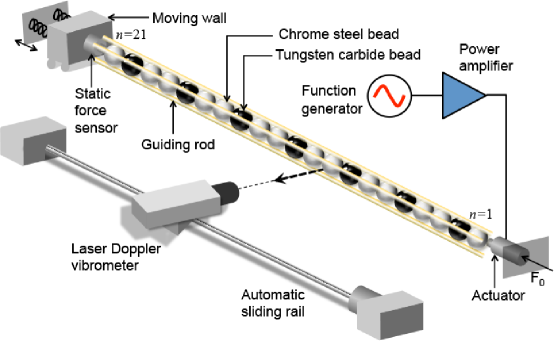
Figure 1: (Color online) Experimental setup of a 21-particle granular chain composed of chrome steel and tungsten carbide beads in a 2:1 ratio. Actuation and sensing systems based on a piezoelectric force sensor and a laser Doppler vibrometer are also illustrated.

Figure 1 shows a schematic of the experimental setup consisting of a granular chain and a laser Doppler vibrometer. In this study, we consider a granular chain composed of $N=21$ spherical beads. The beads are made out of chrome steel (S: gray particles in Fig. 1) and tungsten carbide (W: black particles) materials. See Table 1 for nominal values of the material parameters used hereafter. The granular chain has a spatial periodicity of three particles, and each unit cell follows the pattern of a 2:1 trimer: $\textrm{S}-\textrm{W}-\textrm{S}$. The spheres are supported by four polytetrafluoroethylene (PTFE) rods, which allow axial vibrations of particles with minimal friction, while restricting their lateral movements. The granular chain is compressed by a moving wall at one end of the chain that applies static force in a controllable manner via a linear stage (see Fig. 1). We measure the pre-applied static force ($F_{0}$ = 10 N in this study) by using a static force sensor mounted on the moving wall. We assume that this moving wall is stationary throughout our analysis, since it exhibits orders-of-magnitude larger inertia compared to the particle’s mass.

The granular chain is driven by a piezoelectric actuator positioned on the other side of the chain. We impose actuation signals of chosen amplitude and frequency through an external function generator and a power amplifier. The dynamics of individual particles are scoped by a laser Doppler vibrometer (LDV, Polytec, OFV-534), which is capable of measuring particles’ velocities with a resolution of 0.02 $\mu$m/s/Hz^1/2. The LDV scans the granular chain through the automatic sliding rail and measures the vibrational motions of each particle three times for statistical purposes. We obtain the full-field map of the granular chain’s dynamics by synchronizing and reconstructing the acquired data.

Table 1: Parameter values of the trimer granular chain $(\textrm{S}-\textrm{W}-\textrm{S})$.

	$E\,[\textrm{N}/\textrm{m}^{2}]$	$r\,[\textrm{m}]$	$\nu$	$\rho\,[\textrm{kg}/\textrm{m}^{3}]$
Chrome steel (S)	$200\times 10^{9}$	$9.525\times 10^{-3}$	$0.3$	$7780$
Tungsten Carbide (W)	$628\times 10^{9}$	$9.525\times 10^{-3}$	$0.28$	$14980.64$

III Theoretical Setup

The equation we use to model the experimental setup is a Fermi-Pasta-Ulam-type lattice with a Hertzian potential Nesterneko_book leading to:

$$\ddot{u}_{n}=\frac{A_{n-1}}{M_{n}}\left[\delta_{0,n-1}+u_{n-1}-u_{n}\right]^{3/2}_{+}-\frac{A_{n}}{M_{n}}\left[\delta_{0,n}+u_{n}-u_{n+1}\right]^{3/2}_{+}-\frac{\dot{u}_{n}}{\tau},$$ (1)

where $n=1,\dots,N$, $u_{n}=u_{n}(t)\in{\mathbb{R}}$ is the displacement of the $n$-th bead from its equilibrium position at time $t\in{\mathbb{R}}$, $M_{n}$ is the mass of the $n$-th bead, $\delta_{0,n}$ is a precompression factor induced by the static force $F_{0}=A_{n}\delta_{0,n}^{3/2}$ and the bracket is defined by $[x]_{+}=\max(0,x)$. The $3/2$ power accounting for the nonlinearity of the model is a result of the sphere-to-sphere contact, i.e., the so-called Hertzian contact Hertz. The form of the dissipation is a dash-pot, which has been utilized in the context of granular crystals in several previous works Nature11; dark2. The strength of the dissipation is captured by the parameter $\tau$, which serves as the sole parameter used to fit experimental data ($\tau=2.1$ ms in this study). The elastic coefficient $A_{n}$ depends on the interaction of bead $n$ with bead $n+1$ and for spherical point contacts has the form Johnson_contact

$$A_{n}=\frac{4E_{n}E_{n+1}\sqrt{\frac{r_{n}r_{n+1}}{\left(r_{n}+r_{n+1}\right)}}}{3E_{n+1}\left(1-\nu_{n}^{2}\right)+3E_{n}\left(1-\nu_{n+1}^{2}\right)},$$ (2)

where $E_{n}$, $\nu_{n}$ and $r_{n}$ are the Young’s modulus, Poisson’s ratio and the radius, respectively, of the $n$-th bead. The left boundary is an actuator and the right one is kept fixed, i.e.,

$$u_{0}(t)=a\cos(2\pi f_{b}t),\qquad u_{N+1}(t)=0,$$ (3)

where $a$ and $f_{b}$ represent the driving amplitude and frequency, respectively. Note that at the boundaries (i.e., $n=0$ and $n=N+1$), we consider flat surface-sphere contacts while the same material properties are assumed; thus, e.g., the elastic coefficient at the left boundary takes the form

$$A_{0}=\frac{2E_{1}\sqrt{r_{1}}}{3\left(1-\nu_{1}^{2}\right)}.$$ (4)

III.1 Linear regime and dispersion relation

Assuming dynamic strains that are small relative to the static precompression, i.e.,

$$\frac{|u_{n}-u_{n+1}|}{\delta_{0,n}}\ll 1$$ (5)

Eq. (1) can be well approximated by its linearized form

$$\ddot{u}_{n}=\frac{K_{n-1}}{M_{n}}\left(u_{n-1}-u_{n}\right)-\frac{K_{n}}{M_{n}}\left(u_{n}-u_{n+1}\right)-\frac{\dot{u}_{n}}{\tau},$$ (6)

with ${K_{n}=3/2\,A_{n}\delta_{0,n}^{1/2}}$ corresponding to the linearized stiffnesses. Subsequently, Eq. (6) can be converted into a system of $2N$ first-order equations and written conveniently in matrix form as

$$\dot{\mathbf{Y}}=\mathcal{A}\,\mathbf{Y},$$ (7)

with $\mathbf{Y}=\Big{(}u_{1},\dots,u_{N},\varv_{1}\left(=\dot{u}_{1}\right),\dots,\varv_{N}\left(=\dot{u}_{N}\right)\Big{)}^{T}$ and

$$\mathcal{A}=\pmatrix{}{O}&\mathbf{I}\\ \mathcal{C}(-1/\tau)\,\mathbf{I},$$ (8)

where $\mathbf{O}$ and $\mathbf{I}$ represent the $N\times N$ zero and identity matrices, respectively, and the $N\times N$ (tridiagonal) matrix $\mathcal{C}$ is given by

$$\mathcal{C}=\pmatrix{-}\frac{K_{0}+K_{1}}{M_{1}}&\frac{K_{1}}{M_{1}}0\cdots 0\\ \frac{K_{1}}{M_{2}}-\frac{K_{1}+K_{2}}{M_{2}}\frac{K_{2}}{M_{2}}\vdots\\ 0\ddots\ddots\ddots 0\\ \vdots\frac{K_{N-2}}{M_{N-1}}-\frac{K_{N-2}+K_{N-1}}{M_{N-1}}\frac{K_{N-1}}{M_{N-1}}\\ 0\cdots 0\frac{K_{N-1}}{M_{N}}-\frac{K_{N-1}+K_{N}}{M_{N}}.$$ (9)

Note that in the above linearization we applied fixed boundary conditions at both ends of the chain, i.e., $u_{0}=u_{N+1}=0$ (we account for the actuator in the following subsection). This equation is solved by $Y_{n}=y_{n}e^{i\omega t}$, where $\omega$ corresponds to the angular frequency (with $\omega=2\pi f$) and where,

$$\mathcal{A}\,\mathbf{y}=\lambda\mathbf{y},$$ (10)

with $\left(\lambda,\mathbf{y}\right)$ corresponding to the eigenvalue-eigenvector pair, while $\lambda=i\omega$ and $\mathbf{y}=\left(y_{1},\dots,y_{2N}\right)^{T}$. The eigenfrequency spectrum $\left(f=-i\frac{\lambda}{2\pi}\right)$ using the values of Table 1 and $\tau=2.1\,\textrm{ms}$ is shown in Fig. 2.

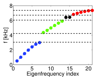
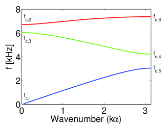
Figure 2: (Color online) Eigenfrequency spectrum of the trimer granular chain for parameter values given in Table 1 and $\tau=2.1$ ms. (a) Spectrum corresponding to Eq. (10) for $N=21$ beads. Note that the horizontal dashed black lines correspond to the cut-off frequencies listed in Table 2. (b) Numerically obtained frequencies of the infinite lattice using Eq. (18) as a function of the wavenumber $(k\alpha)$.

On the other hand, the dispersion relation for the trimer chain configuration within an infinite lattice can be obtained using a Bloch wave ansatz Tun_Band_gaps. We first re-write Eq. (6) in the following convenient form

$$\ddot{u}_{3j-2} = \frac{K_{3}}{M_{1}}\left(u_{3j-3}-u_{3j-2}\right)-\frac{K_{1}}{M_{1}}\left(u_{3j-2}-u_{3j-1}\right)-\frac{\dot{u}_{3j-2}}{\tau},$$ (11)

$$\ddot{u}_{3j-1} = \frac{K_{1}}{M_{2}}\left(u_{3j-2}-u_{3j-1}\right)-\frac{K_{1}}{M_{2}}\left(u_{3j-1}-u_{3j}\right)-\frac{\dot{u}_{3j-1}}{\tau},$$ (12)

$$\ddot{u}_{3j} = \frac{K_{1}}{M_{1}}\left(u_{3j-1}-u_{3j}\right)-\frac{K_{3}}{M_{1}}\left(u_{3j}-u_{3j+1}\right)-\frac{\dot{u}_{3j}}{\tau},$$ (13)

with $j\in{\mathbb{Z}}^{+}$, where we made use of the spatial periodicity of the trimer lattice, i.e., $M_{3j}=M_{3j-2}\equiv M_{1}(=M_{3})$ and $K_{3j-2}=K_{3j-1}\equiv K_{1}(=K_{2})$, and $M_{3j-1}\equiv M_{2}$ and $K_{3j}\equiv K_{3}$. The Bloch wave ansatz has the form,

$$u_{3j-2}=u_{0}e^{i\left(k\alpha j+\omega t\right)},$$ (14)

$$u_{3j-1}=v_{0}e^{i\left(k\alpha j+\omega t\right)},$$ (15)

$$u_{3j}=w_{0}e^{i\left(k\alpha j+\omega t\right)},$$ (16)

where $u_{0},v_{0}$ and $w_{0}$ are the wave amplitudes, $k$ is the wavenumber and $\alpha$ is the size (or the equilibrium length) of one unit cell of the lattice. Substitution of Eqs. (III.1) into Eqs. (III.1) yields

$$\pmatrix{\omega}^{2}-\frac{K_{1}+K_{3}}{M_{1}}-i\frac{\omega}{\tau}&\frac{K_{1}}{M_{1}}\frac{K_{3}}{M_{1}}e^{-ik\alpha}\\ \frac{K_{1}}{M_{2}}\omega^{2}-\frac{2K_{1}}{M_{2}}-i\frac{\omega}{\tau}\frac{K_{1}}{M_{2}}\\ \frac{K_{3}}{M_{1}}e^{ik\alpha}\frac{K_{1}}{M_{1}}\omega^{2}-\frac{K_{1}+K_{3}}{M_{1}}-i\frac{\omega}{\tau}\pmatrix{u}_{0}\\ v_{0}\\ w_{0}=\pmatrix{0}\\ 0\\ 0.$$ (17)

The non-zero solution condition of the matrix-system (17), or dispersion relation (i.e., the vanishing of the determinant of the above homogeneous linear system), has the form

$$M_{1}^{2}M_{2}\omega^{6}-i\frac{3M_{1}^{2}M_{2}}{\tau}\omega^{5}-M_{1}\left[2\left[K_{3}M_{2}+K_{1}\left(M_{1}+M_{2}\right)\right]+\frac{3M_{1}M_{2}}{\tau^{2}}\right]\omega^{4}$$

$$+i\frac{M_{1}}{\tau}\left[4\left[K_{3}M_{2}+K_{1}\left(M_{1}+M_{2}\right)\right]+\frac{M_{1}M_{2}}{\tau^{2}}\right]\omega^{3}-4K_{1}^{2}K_{3}\sin^{2}{\left(\frac{k\alpha}{2}\right)}$$

$$+\left[K_{1}\left(K_{1}+2K_{3}\right)\left(2M_{1}+M_{2}\right)+\frac{2M_{1}}{\tau^{2}}\left[K_{3}M_{2}+K_{1}\left(M_{1}+M_{2}\right)\right]\right]\omega^{2}$$

$$-i\frac{K_{1}}{\tau}\left(K_{1}+2K_{3}\right)\left(2M_{1}+M_{2}\right)\omega=0,$$ (18)

which has (non-trivial) solutions at $k=0$ and $k=\pi/\alpha$ (i.e., first Brillouin zone) given by

(19)

(20)

where~f

=[K_1(2M_1+M_2)+2K_3M_2]^2-16K_1K_3M_1M_2$.Thesolutions(\ref{cut_off_freq})correspondtothe\textit{cut-off frequencies}ofthespectralbands.Theabovevaluesare(inprinciple)complexsinceweconsiderdissipativedynamicsinthesystem~{}(\ref{gc_start})(embodiedbythe$˙u_n/τ$term)inordertomodeltheexperimentalsetup.Therefore,thereportedfrequencieshereafterwillcorrespondtothe\textit{real}partofthesevalues,i.e.,thepartcontributingtothedispersionpropertiesofthesolutionsratherthantheirdecay.InTable~{}\ref{cut_off_freq_values},thepredictedvaluesofthecut-offfrequenciesarepresented(uptotwodecimalplaces)usingthevaluesofthematerialparametersofTable~{}\ref{gc_params}and$τ= 2.1$ms.\par Finally,uponsolvingnumericallythedispersionrelation(cf.Eq.~{}(\ref{dispersion_relation})),thefrequencyasafunctionofthewavenumber($κα$)ispresentedinFig.~{}\ref{fig1b}togetherwiththecut-offfrequenciesofTable~{}\ref{cut_off_freq_values}.Notethatthesecut-offfrequenciesarealsoplottedashorizontaldashedblacklinesinFig.~{}\ref{fig1a}forcomparison.ItcanbediscernedfrombothpanelsofFig.~{}\ref{fig1}thatthereexisttwofinitegapsinthefrequencyspectrum(ingeneraltheirnumberisonelessthantheperiodofthegranularcrystal),namely,$[f_c,5,f_c,4]$and$[f_c,3,f_c,2]$,togetherwithonesemi-infinitegap$[f_c,6,∞)$.WealsonotethepresenceoftwoadditionallocalizedmodesdepictedinFig.~{}\ref{fig1a}betweenthefirstandsecondopticalpassbandsduetothefixedboundaryconditions.Thesemodes,denotedbyblackdotsinFig.~{}\ref{fig1a},correspondtosurfacemodesandtheirexistencehasbeenpreviouslydiscussed,e.g.,in~{}\cite[cite]{\@@bibref{Authors Phrase1YearPhrase2}{Theo2010}{\@@citephrase{(}}{\@@citephrase{)}}}.\par\par\begin{table}[h]\@@toccaption{{\lx@tag[ ]{{2}}{Calculatedcut-offfrequencies(in$\textrm{kHz}$)usingEqs.~{}(\ref{cut_off_freq}).}}}\@@caption{{\lx@tag[: ]{{Table 2}}{Calculatedcut-offfrequencies(in$\textrm{kHz}$)usingEqs.~{}(\ref{cut_off_freq}).}}}\centering\begin{tabular}[]{| c | c | c | c | c |}\hline\cr$f_{c,5}$&$f_{c,4}$&$f_{c,3}$&$f_{c,2}$&$f_{c,6}$\\ \hline\cr\hline\cr$3.04$&$4.23$&$6.04$&$6.71$&$7.37$\\ \hline\cr\end{tabular}\@add@centering\end{table}\par\par$

III.2 Steady-state analysis in the linear regime

In order to account for the actuation in the linear problem we add an external forcing term to Eq. (7) in the form,

$$\dot{\mathbf{Y}}=\mathcal{A}\,\mathbf{Y}+\mathbf{F}(\omega_{b}),$$ (23)

where the sole non-zero entry of $\mathbf{F}(\omega_{b})$ is at the $(N+1)$th node and has the form $F_{N+1}=a\cos{\left(\omega_{b}t\right)}$ and the matrix $\mathcal{A}$ is given by Eq. (8). Equation (23) can be solved by introducing the ansatz

$$\mathbf{Y}=\pmatrix{}{aligned}a_{1}\cos$$ (24)

&+b1sin(ωbt) ⋮ aNcos(ωbt)+bNsin(ωbt) -a1ωbsin(ωbt)+b1ωbcos(ωbt) ⋮ -aNωbsin(ωbt)+bNωbcos(ωbt) ,withunknown(real)parametersa_jandb_j(j=1,⋯,N).InsertingEq.(

III.2)intoEq.(23)yieldsasystemoflinearequationswhichcanbeeasilysolved:

$$\widetilde{\mathcal{A}}\,\mathbf{X}=\widetilde{\mathbf{F}},$$ (25)

where

$$\widetilde{\mathcal{A}}=\pmatrix{\widetilde{\hfil}}$$ (26)

&(ω/τ)I -(ω/τ)I~C,~C=-(C+ω_b^2 I)withCgivenbyEq.(

9),whileX=(a_1,…,a_N,b_1,…,b_N)isthevectorcontainingtheunknowncoefficientsand~F=(a K0M1,0,…,0).WerefertoEq.(III.2)astheasymptoticequilibriumofthelinearproblem(asdictatedbytheactuator),sinceallsolutionsofthelinearproblemapproachitfort →∞.Clearly,thisstatewillbespatiallylocalizediftheforcingfrequencyf_blieswithinaspectralgap,otherwiseitwillbespatiallyextended(withtheformercorrespondingtoasurfacebreather,whichwediscussinthefollowingsection).Forsmalldrivingamplitudea,wefindthatthelong-termdynamicsofthesystemapproachesanasymptoticstatethatisreasonablywellapproximatedbysteadystatelinansatz.However,forlargerdrivingamplitudestheeffectofthenonlinearitybecomessignificant,andwecannolongerrelyonthelinearanalysis.

Inordertounderstandthedynamicsinthehigh-amplituderegime,weperformabifurcationanalysisoftime-periodicsolutionsofthenonlinearproblem

gcstartusingaNewton-Raphsonmethodthatyieldsexacttime-periodicsolutions(toaprescribedtolerance)andtheirlinearstabilitythroughthecomputationofFloquetmultipliers(seeAppendix

LABEL:sec:app_num_methodsfordetails).WeusetheasymptoticlinearstatesteadystatelinansatzasaninitialguessfortheNewtoniterations.

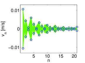
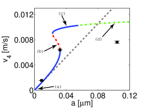
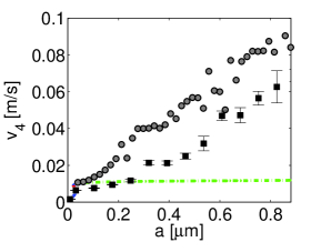
Figure 3: (Coloronline)Comparisonbetweenexperimentalandtheoreticalresultsforadrivingfrequencyf_b=6.3087 kHz,whichliesinthesecondspectralgap.(a)Profileofsolutionforadrivingamplitudeofa=32.16 nm.Experimentalvalues(greenshadedareas)areshownasasuperpositionofthevelocitiesmeasuredoverthe50 mstimewindowofrecordeddata.Thenumericallypredictedextrema(overoneperiod)oftheexactsolutionobtainedviaNewton′smethodareshownwithblue(open)circles.(b)Thequantityv_4asafunctionoftheamplitudeaofthedrive.Forthenumericallyexactsolutions,v_4isthemaximumvelocityofthe4thbeadoveroneperiodofmotion.Notethatthebluesegmentscorrespondtostableparametricregionswhiletheredandgreenonescorrespondtorealandoscillatoryunstableparametricregions,respectively.Blacksquareswitherrorbarsrepresenttheexperimentallymeasuredmeanvaluesofthequantityv_4overthreeexperimentalruns,wherev_4wascalculatedasthemaximummeasuredoverthe50 mstimewindowofrecordeddata.Finally,thedashedgraylineisthemaximumvelocity(overoneperiod)ofbead4aspredictedbythelinearsolutionofEq.(III.2).(c)Zoomedoutversionofpanel(b).Thegraycirclescorrespondtonumericalresultsthatwereobtainedbydynamicallyrunningtheequationsofmotionandmonitoringthemaximumvelocityv_4overtheexperimentaltimewindow.Theexperimentaldatainthispanelareshownagainbyblacksquares.

IV MainResults

Besidesthelinearlimitconsideredabove,anotherrelevantsituationisthatoftheHamiltoniansystem,i.e.,with1/τ→0inEq.

gcstartanda →0inEq.(

3).Itiswellknownthattime-periodicsolutionsthatarelocalizedinspace(i.e.,breathers)existinahostofdiscreteHamiltoniansystemsFlach2007,includinggranularcrystalswithspatialperiodicityTheo2010.Inparticular,Hamiltoniantrimergranularchainswererecentlystudiedinhooge13.There,itwasobservedthatbreatherswithfrequencyinthesecondspectralgaparemorerobustthanthosewithfrequencyinthefirstspectralgap.Featuresthatappeartoenhancethestabilityofthehighergapbreathersare(i)tailsavoidingresonanceswiththespectralbandsand(ii)lighterbeadsoscillatingout-of-phase.Inthatsense,thebreathersfoundinthesecondspectralgapoftrimersaresomewhatreminiscentofbreathersfoundinthegapofdimerlatticesTheo2010.Furthermore,breathersofdamped-drivendimergranularcrystals(i.e.,Eq.gcstartwithaspatialperiodicityoftwo)werestudiedrecentlyinhooge12.Inthatsetting,thebreathersbecomesurface breatherssincetheyarelocalizedatthesurface,ratherthanthecenterofthechain.Yet,ifonetranslatesthesurfacebreathertothecenterofthechain,itbearsastrongresemblancetoa``bulk"breather.Thus,nonlinearity,periodicityanddiscretenessenabledtwoclassesofrelevantstates:Thenonlinearsurfacebreathersandonestunedtotheexternalactuator(i.e.,thoseproximaltotheasymptoticlinearstatedictatedbytheactuator).Thesetwowaveformswereobservedtocollideanddisappearinalimitcyclesaddle-nodebifurcationastheactuationamplitudewasincreasedhooge12.Beyondthiscriticalpoint,nostable,periodicsolutionswerefoundtoexistinthedimercaseofhooge12andthedynamicswerefoundto``jump"toachaoticbranch.Weaimtoidentifysimilarfeaturesinthecaseofthetrimerwithaparticularemphasisonthedifferencesarisingduetothehigherorderperiodicityofthesystem.Tothatend,wefirstpresentresultsonsurfacebreatherswithfrequencyinthesecondgap,andperformparametercontinuationindrivingamplitudetodrawcomparisonstothebifurcationstructureindimergranularlattices.Followingthat,weinvestigatebreathersinthefirstspectralgapandcomparethemtotheirsecondgapbreathercounterparts.Finallyweidentifybothlocalizedandspatiallyextendedstatesasthedrivingfrequencyisvariedthroughtheentirerangeofspectralvaluescoveringbothgapsandthethreepassbandsbetweenwhichtheyarise.

IV.1 Drivinginthesecondspectralgap

Wefirstconsiderafixeddrivingfrequencyoff_b = 6.3087kHz,whichlieswithinthesecondspectralgap(seeTableII).Forlowdrivingamplitudethereisasingletime-periodicstate(i.e.,theoneproximaltothedrivenlinearstate),whichtheexperimentallyobserveddynamicsfollows(seepanels(a)and(b)inFig.

3).Acontinuationindrivingamplitudeofnumericallyexacttime-periodicsolutions(seetheblue,redandgreenlinesofFig.3),revealstheexistenceofthreebranchesofsolutionsforarangeofdrivingamplitudes.Thebranchindicatedbylabel(a)isproximaltothelineardrivenstategivenbyEq.steadystatelinansatz(shownasagraydashedlineinFig.3).Eachsolutionmakingupthisbranchisin-phasewiththeboundaryactuator(seeFig.4),andhaslightermassesthatareout-of-phasewithrespecttoeachother(seee.g.,Fig.LABEL:ra).Thesesolutionsareasymptoticallystable,whichisalsoevidentintheexperiments(seeFig.3andtheblackmarkerswitherrorbarsinFig.3).Atadrivingamplitudeofa≈22.75 nm,anunstableandstablebranchofnonlinearsurfacebreathersarisethroughasaddle-nodebifurcation(seelabels(b)and(c)ofFig.3,respectively).Atthebifurcationpointa≈22.75 nm,theprofilestronglyresemblesthatofthecorrespondingHamiltonianbreather(whenshiftedtothecenterofthechain),hencethenamesurfacebreather.Itisimportanttonotethatthepresenceofdissipationdoesnotallowforthisbranchtobifurcateneara →0(wherethisbifurcationwouldoccurintheabsenceofdissipation).Instead,theneedofthedrivetoovercomethedissipationensuresthatthebifurcationwillemergeatafinitevalueofa.Asaisincreased,thesolutionsconstitutingtheunstable``separatrix′′branch(b)resembleprogressivelymoretheonesofbranch(a);seeFig.4.Forexample,branch(b)progressivelybecomesin-phasewiththeactuatorasaisincreased.Indeedthesetwobranchescollideandannihilateata≈32.26 nm.Ontheotherhand,the(stable,atleastforaparametricintervalina)nonlinearsurfacebreather(c)isout-of-phasewiththeactuator(seeFig.4).ThissolutionlosesitsstabilitythroughaNeimark-Sackerbifurcation,whichistheresultofaFloquetmultiplier(lyingofftherealline)acquiringmodulusgreaterthanunity,(seelabel(d)ofFig.3andFig.4).SuchaFloquetmultiplierindicatesconcurrentgrowthandoscillatorydynamicsofperturbationsandthustheinstabilityisdeemedasanoscillatoryone.SolutionswithanoscillatoryinstabilityaremarkedingreeninFig.3,whereasreddashedlinescorrespondtopurelyrealinstabilities(seealsoFig.4asacaseexample)andsolidbluelinesdenoteasymptoticallystableregions.Thereasonformakingthedistinctionbetweenrealandoscillatoryinstabilitiesisthatquasi-periodicityandchaosoftenlurkinregimesinparameterspacewheresolutionspossesssuchinstabilitieshooge12.Indeed,pasttheabovesaddle-nodebifurcation,astheamplitudeisfurtherincreased,foranadditionalnarrowparametricregime,thecomputationaldynamics(graycirclesinFig.3)followstheuppernonlinearsurfacemodeofbranch(c);yet,oncethisbranchbecomesunstablethedynamicsappearstoreachachaoticstate.Intheexperimentaldynamics(blacksquaresinFig.3),averysimilarpatternisobservedqualitatively,althoughthequantitativedetailsappeartosomewhatdiffer.Admittedly,asthemorenonlinearregimesofthesystem′sdynamicsareaccessed(asaincreases),suchdisparitiesareprogressivelymorelikelyduetotheopeningofgapsbetweenthespheresandthelimitedapplicability(insuchregimes)ofthesimpleHertziancontactlaw.

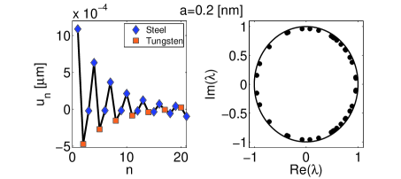
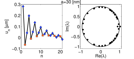
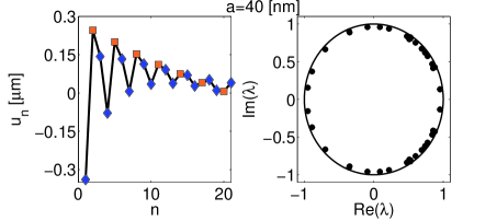
Figure 4: (Coloronline)DisplacementprofilesandcorrespondingFloquetmultipliersoftime-periodicsolutionsobtainedatadrivingfrequencyoff_b=6.3087  kHzforadrivingamplitudeof(a)a = 0.2 nm,(b)a = 30  nm,(c)a=40 nmand(d)a = 0.1 $\mu$m.Thesesolutionscorrespondtothe(a)-(d)labelsofFig.3.Thelightermasses(i.e.,theSteelbeads)oscillate(nearly)out-of-phaseandareshownasbluediamondswhereastheheaviermasses(theTungstenCarbideones)areshownasorangesquares.