clustvarsel: A Package Implementing Variable Selection for Model-based Clustering in R

Abstract

Finite mixture modelling provides a framework for cluster analysis based on parsimonious Gaussian mixture models. Variable or feature selection is of particular importance in situations where only a subset of the available variables provide clustering information. This enables the selection of a more parsimonious model, yielding more efficient estimates, a clearer interpretation and, often, improved clustering partitions. This paper describes the R package clustvarsel which performs subset selection for model-based clustering. An improved version of the methodology of Raftery and Dean (2006) is implemented in the new version 2 of the package to find the (locally) optimal subset of variables with group/cluster information in a dataset. Search over the solution space is performed using either a stepwise greedy search or a headlong algorithm. Adjustments for speeding up these algorithms are discussed, as well as a parallel implementation of the stepwise search. Usage of the package is presented through the discussion of several data examples.

Keywords: model-based clustering, BIC, subset selection, R.

1 Introduction

Cluster analysis is the search for a priori unknown group structure in data. Model-based clustering is increasingly becoming one of the most popular cluster analysis methods. Model-based clustering is based on Finite mixture models (McLachlan and Peel, 2000), with each component density usually representing a cluster. For continuous data, Gaussian components are usually used to model clusters. Model-based clustering as implemented in the R package mclust (Fraley et al., 2012) allows for automatic selection of the number of components, and selection of parsimonious covariance structures.

In cluster analysis, as in classification or other supervised learning tasks, the inclusion of noise variables, i.e. features without useful group information, can severely degrade the final results. In fact, the presence of noise variables can negatively impact both the estimation of the number of clusters in the data and the recovery of those groups. The new clustvarsel (version $\geq 2.0$) R package implements a wrapper method for automatic variable selection in model-based clustering (as implemented in the mclust package). Thus, the addition of the clustvarsel package allows for automatic variable selection to be included in the estimation process.

Raftery and Dean (2006) introduced a stepwise variable selection methodology tailored to model-based clustering. An earlier version of clustvarsel (version 1) implemented this methodology. Variables designated as noise variables in this process were not required to be independent of the clustering variables. However, noise variables could be conditionally independent of the clustering, but still linearly dependent on the clustering variables. This linear dependency was modelled using linear regression.

Maugis et al. (2009a) extended the framework of Raftery and Dean (2006) by allowing the noise variables to depend on a (possibly null) subset of the clustering variables via stepwise variable selection in the linear regression (see also Maugis et al., 2009b). This allows for a more parsimonious modelling of the relationship between the noise variables and the clustering variables. For more detail on the variable selection framework from both Raftery and Dean (2006) and Maugis et al. (2009a) see Section 2.

Section 3 introduces the main function in the clustvarsel package, and discusses the options for the available arguments. In Section 4, several examples are presented by applying the methodology to both synthetic and real world datasets. Algorithmic speedups are discussed in Section 5, including a description of a parallel implementation of the stepwise greedy search in Section 5.3. The paper concludes with some discussion and final remarks in Section 6.

2 Methodology

Model-based clustering assumes that the observed data are generated from a mixture of $G$ components, each representing the probability distribution for a different group or cluster (McLachlan and Peel, 2000; Fraley and Raftery, 2002). For continuous data, the density of each mixture component can be described by the multivariate Gaussian distribution. Thus, the general form of a Gaussian finite mixture model is

$$f(\boldsymbol{x})=\sum_{g=1}^{G}\pi_{g}\phi(\boldsymbol{x}|\boldsymbol{\mu}_{g},\boldsymbol{\Sigma}_{g}),$$

where $\pi_{g}$ represents the mixing probabilities, so that $\pi_{g}>0$ and $\sum_{g=1}^{G}\pi_{g}=1$, $\phi(\cdot)$ is the multivariate Gaussian density with parameters $(\boldsymbol{\mu}_{g},\boldsymbol{\Sigma}_{g})$ ($g=1,\ldots,G$). Clusters are ellipsoidal, centred at the mean vector $\boldsymbol{\mu}_{g}$, with other geometric features, such as volume, shape and orientation, determined by $\boldsymbol{\Sigma}_{g}$. Parsimonious parameterisation of covariance matrices is available through the eigenvalue decomposition $\boldsymbol{\Sigma}_{g}=\lambda_{g}\boldsymbol{D}_{g}\boldsymbol{A}_{g}\boldsymbol{D}^{\top}_{g}$, where $\lambda_{g}$ is a scalar controlling the volume of the ellipsoid, $\boldsymbol{A}_{g}$ is a diagonal matrix specifying the shape of the density contours, and $\boldsymbol{D}_{g}$ is an orthogonal matrix which determines the orientation of the corresponding ellipsoid (Banfield and Raftery, 1993; Celeux and Govaert, 1995). Fraley et al. (2012, Table 1) report some parameterisation of within-group covariance matrices available in the R package mclust, and the corresponding geometric characteristics.

Raftery and Dean (2006) discussed the problem of variable selection for model-based clustering by recasting the problem as a model selection procedure. Their proposal is based on the use of BIC to approximate Bayes factors to compare mixture models fitted on nested subsets of variables. A generalisation of their approach was later discussed by Maugis et al. (2009a, b).

Let us suppose that the set of available variables, $\mathcal{X}$, is partitioned into three disjoint parts: the set of previously selected variables, $\mathcal{X}_{\text{clust}}$, the variable under consideration for inclusion or exclusion from the active set, $X_{i}$, and the set of the remaining variables, $\mathcal{X}_{\text{other}}\equiv\mathcal{X}\setminus\{\mathcal{X}_{\text{clust}}\cup X_{i}\}$.

Raftery and Dean (2006) showed that the inclusion (or exclusion) of variables can be assessed using the following BIC difference:

$$\text{BIC}_{\text{diff}}=\text{BIC}_{\text{clust}}(\mathcal{X}_{\text{clust}},X_{i})-\text{BIC}_{\text{not\,clust}}(\mathcal{X}_{\text{clust}},X_{i}),$$ (1)

where $\text{BIC}_{\text{clust}}(\mathcal{X}_{\text{clust}},X_{i})$ is the BIC value for the “best” clustering mixture model (i.e. assuming $G\geq 2$) fitted using the features set $\{\mathcal{X}_{\text{clust}}\cup X_{i}\}$, whereas $\text{BIC}_{\text{not\,clust}}(\mathcal{X}_{\text{clust}},X_{i})$ is the BIC value for no clustering for the same set of variables. The latter can be written as

$$\text{BIC}_{\text{not\,clust}}(\mathcal{X}_{\text{clust}},X_{i})=\text{BIC}_{\text{clust}}(\mathcal{X}_{\text{clust}})+\text{BIC}_{\text{reg}}(X_{i}|\mathcal{X}_{\text{clust}}),$$ (2)

i.e. the BIC value for the “best” clustering model fitted using the set $\mathcal{X}_{\text{clust}}$ plus the BIC value for the regression of the candidate variable $X_{i}$ on the variables included in the set $\mathcal{X}_{\text{clust}}$.

The difference in BIC score (1) is an approximation of the log of the Bayes factor comparing the model where the variable under consideration, $X_{i}$, is a clustering variable with the model where the variable is conditionally independent of the clustering. Large, positive values of $\text{BIC}_{\text{diff}}$ can be taken as an evidence that variable $X_{i}$ is useful for clustering.

In all clustering models, the “best” model is identified with respect to the number of mixture components (assuming $G\geq 2$) and to model parameterisations. In the linear regression model term, $X_{i}$ can depend on all the variables in $\mathcal{X}_{\text{clust}}$, a subset of them, or none (complete independence). Finally, note that in both equations (1) and (2) the set of remaining variables, $\mathcal{X}_{\text{other}}$, plays no role. For more details of the methodology see Raftery and Dean (2006), and for improvements due to the subset selection in the regression model see Maugis et al. (2009a).

Practical implementation of the above methodology requires the use of an algorithm for checking single variables for inclusion/exclusion from the set of selected clustering variables. A stepwise greedy search algorithm checks the inclusion of each single variable not currently selected into the current set of selected clustering variables at each step. The variable that has the highest evidence of inclusion is proposed and, if its clustering evidence is stronger than the evidence against clustering, it is included. At every exclusion step, the algorithm checks the removal of each single variable in the currently selected set of clustering variables, and proposes the variable that has the lowest evidence of clustering. The proposed variable is removed if the evidence for its being a clustering variable is weaker than the evidence against. This is similar to the idea for stepwise regression and may suffer from the same instabilities mentioned in Miller (1990) inherent in that approach (although this has not been apparent in the simulations and examples tried thus far).

The stepwise algorithm can be implemented in a forward/backward fashion, i.e. starting from the empty set of clustering variable and then continuing to add or remove features until there is no evidence of further clustering variables. It can also be implemented in a backward/forward fashion, i.e. starting from the full set of features as clustering variables and then continuing to remove or add features until there is no evidence of further clustering variables.

Another possible algorithm is the headlong search, which involves potentially checking less variables at each inclusion or exclusion step, and so may be quicker than the stepwise greedy search (at a possible price in terms of performance) for use on datasets with a large number of variables. At each inclusion step, the headlong algorithm only checks single variables not currently in the set of clustering variables until the difference between the BIC for clustering versus not clustering is above a pre-specified upper level (a default value of 0 implies that the evidence for clustering is greater than that for not clustering).

Because the algorithm stops once this criterion is satisfied, it will not necessarily check all the variables available, and the variable selected will not necessarily be the best possible feature at that step. Any variables that are checked during this step, whose difference between the BIC for clustering versus not clustering is below a pre-specified lower level, are removed from consideration for the rest of the algorithm (a default value of $-10$ means that there is a strong evidence against clustering). Because of this, possibly irrelevant variables can be removed early on in the algorithm and further reduce the number of variables checked at each step.

Similarly, at each exclusion, the algorithm only checks single variables currently in the set of clustering variables until the BIC difference for clustering versus not clustering is below the pre-specified upper level. The algorithm stops checking once a variable satisfies this criterion, and that variable is removed from the set. If the difference in BIC is smaller than the lower level, then the variable is removed from consideration for the rest of the algorithm, otherwise it can still be checked in future inclusion/exclusion steps. See Badsberg (1992) for full details about the headlong algorithm.

3 The R package clustvarsel

The clustvarsel package can be used to find the (locally) optimal subset of variables with group/cluster information in a dataset with continuous variables. In this section, usage of the main function clustvarsel and its arguments is described.

The clustvarsel package depends on other packages available on CRAN for model fitting (mclust, Fraley et al. (2014)), or for providing some facilities, such as parallelisation (parallel, R Core Team (2014); doParallel, Revolution Analytics and Weston (2013a); foreach, Revolution Analytics and Weston (2013b); iterators, Analytics (2012)), and subset selection in regression models (BMA, Raftery et al. (2013)). By loading the package as usual with library(clustvarsel), it will also take care of making all the other packages available for the current session.

Once the clustvarsel package has been loaded, the main function a user needs to invoke is the following:

clustvarsel(data,            G = 1:9,            search = c("greedy", "headlong"),            direction = c("forward", "backward"),            emModels1 = c("E", "V"),            emModels2 = mclust.options("emModelNames"),            samp = FALSE,            sampsize = round(nrow(data)/2),            hcModel = "VVV",            allow.EEE = TRUE,            forcetwo = TRUE,            BIC.diff = 0,            BIC.upper = 0,            BIC.lower = -10,            itermax = 100,            parallel = FALSE)

The available arguments are:

data

A numeric matrix or data frame where rows correspond to observations and columns correspond to variables. Categorical variables are not allowed.

G

An integer vector specifying the numbers of mixture components (clusters) for which the BIC is to be calculated. The default is G = 1:9.

search

A character vector indicating whether a "greedy" or, potentially quicker but less optimal, "headlong" algorithm is to be used in the search for clustering variables.

direction

A character vector indicating the type of search: "forward" starts from the empty model and at each step of the algorithm adds/removes a variable until the stopping criterion is satisfied; "backward" starts from the model with all the available variables and at each step of the algorithm removes/adds a variable until the stopping criterion is satisfied. For the "headlong" search only the "forward" algorithm is available.

emModels1

A vector of character strings indicating the models to be fitted in the EM phase of univariate clustering. Possible models are "E" and "V", described in help(mclustModelNames).

emModels2

A vector of character strings indicating the models to be fitted in the EM phase of multivariate clustering. Possible models are those described in help(mclustModelNames).

samp

A logical value indicating whether or not a subset of observations should be used in the hierarchical clustering phase used to get starting values for the EM algorithm.

sampsize

The number of observations to be used in the hierarchical clustering subset. By default, a random sample of approximately half of the sample size is used.

hcModel

A character string specifying the model to be used in hierarchical clustering for choosing the starting values used by the EM algorithm. By default, the unconstrained "VVV" covariance structure is used.

allow.EEE

A logical value indicating whether a new clustering will be run with equal within-cluster covariance for hierarchical clustering to get starting values, if the clusterings with variable within-cluster covariance for hierarchical clustering do not produce any viable BIC values.

forcetwo

A logical value indicating whether at least two variables will be forced to be selected initially, regardless of whether BIC evidence suggests bivariate clustering or not.

BIC.diff

A numerical value indicating the minimum BIC difference between clustering and no clustering used to accept the inclusion of a variable in the set of clustering variables in a forward step of the greedy search algorithm. Furthermore, minus BIC.diff is used to accept the exclusion of a selected variable from the set of clustering variable in a backward step of the greedy search algorithm. Default is $0$.

BIC.upper

A numerical value indicating the minimum BIC difference between clustering and no clustering used to select a clustering variable in the headlong search. Default is $0$.

BIC.lower

A numerical value indicating the level of BIC difference between clustering and no clustering below which a variable will be removed from consideration in the headlong algorithm. Default is $-10$.

itermax

An integer value giving the maximum number of iterations (of addition and removal steps) the selected algorithm is allowed to run for.

parallel

This argument allows to specify if the selected "greedy" algorithm should be run sequentially or in parallel. The possible values are:

1. a logical value specifying if parallel computing should be used (TRUE) or not (FALSE, default) for running the algorithm;

2. a numerical value which gives the number of cores to employ (by default, this is obtained from function detectCores in the parallel package);

3. a character string specifying the type of parallelisation to use. The latter depends on system OS: on Windows OS only "snow" type functionality is available, whereas on Unix/Linux/Mac OSX both "snow" and "multicore" (default) functionalities are available.

Options (ii) and (iii) imply that the search is performed in parallel. By default the algorithm is run sequentially.

A basic clustvarsel function call needs to input a matrix or data frame containing the data to analyse. Fine tuning is possible by specifying the arguments described above. The following section presents some examples of its usage in practice.

4 Examples

In this section we present some data analysis examples based on simulated data and on well-known real datasets.

4.1 Simulated data

We consider some of the synthetic data examples described in Maugis et al. (2009a). Samples were simulated for a 10-dimensional feature vector where only the first two variables provide clustering information. These were generated from a mixture of four Gaussian distributions $\boldsymbol{X}_{[1:2]}\sim N(\boldsymbol{\mu}_{k},\boldsymbol{I}_{2})$ with $\boldsymbol{\mu}_{1}=(-2,-2)$, $\boldsymbol{\mu}_{2}=(-2,2)$, $\boldsymbol{\mu}_{3}=-\boldsymbol{\mu}_{2}$, $\boldsymbol{\mu}_{4}=-\boldsymbol{\mu}_{1}$, and mixing probabilities $\pi=(0.3,0.2,0.3,0.2)$. The remaining eight variables were simulated according to the model $\boldsymbol{X}_{[3:10]}=\boldsymbol{X}_{[1:2]}\boldsymbol{\beta}+\epsilon$, where $\epsilon\sim N(\boldsymbol{0},\boldsymbol{\Omega})$. Different settings for $\boldsymbol{\beta}$ and $\boldsymbol{\Omega}$ define seven different scenarios (see Table 1 in Maugis et al., 2009a). These range from independence of clustering variables on the other features (model 1 and 2) to cases of increasing degree of dependence of the irrelevant variables on the clustering ones (model 3 to 7). In the following, we focus only on some of the scenarios. For ease of reading, the values of the parameters for such scenarios are reported in Table 1.

Table 1: Parameter settings for the scenarios used to generated synthetic data: $\boldsymbol{\beta}$ defines the correlation of irrelevant variables on clustering variables, whereas $\boldsymbol{\Omega}$ is the covariance structure of the noise component. $\boldsymbol{0}_{p}$ indicates the $(2\times p)$ matrix of zeroes, and $\boldsymbol{I}_{p}$ the $(p\times p)$ identity matrix.

Scenario	Parameters		Scenario	Parameters
Model 1	$\boldsymbol{\beta}=\boldsymbol{0}_{8}$		Model 5	$\boldsymbol{\beta}=\left(\begin{matrix}0.5&0&2&0\\ 0&1&0&3\end{matrix}\;\boldsymbol{0}_{4}\right)$
	$\boldsymbol{\Omega}=\boldsymbol{I}_{8}$			$\boldsymbol{\Omega}=\operatorname{diag}(\boldsymbol{I}_{2},0.5\boldsymbol{I}_{2},\boldsymbol{I}_{4})$
Model 4	$\boldsymbol{\beta}=\left(\begin{matrix}0.5&0\\ 0&1\end{matrix}\;\boldsymbol{0}_{6}\right)$		Model 7	$\boldsymbol{\beta}=\left(\begin{matrix}0.5&0&2&0&2&0.5&2&0\\ 0&1&0&3&0.5&1&0&3\end{matrix}\right)$
	$\boldsymbol{\Omega}=\boldsymbol{I}_{8}$			$\boldsymbol{\Omega}=\operatorname{diag}(\boldsymbol{I}_{2},0.5\boldsymbol{I}_{4},\boldsymbol{I}_{2})$

The simulation results were evaluated using the following criteria:

• Variable Selection Error Rate (VSER) to assess variable selection performance. VSER is defined as the ratio of the number of errors in selecting (or not selecting) variables to the total number of variables in the set. A perfect recovey of clustering variables gives VSER $=0$, while VSER can be no greater than 1.

• Adjusted Rand Index (ARI, Hubert and Arabie, 1985) to measure classification accuracy. A perfect classification gives ARI $=1$, whereas ARI $=0$ for a random classification.

Table 2 shows the results from a simulation study for the above synthetic data using sample sizes $n=200$ and $n=1000$. The methods compared are MCLUST, the best GMM using the full set of variables, CLUSTVARSEL[fwd] and CLUSTVARSEL[bkw], the best GMM using the subset of relevant clustering variables selected by, respectively, the forward/backward and backward/forward greedy search, and SPARSEKMEANS, a sparse version of $k$-means algorithm (Witten and Tibshirani, 2010). Because the last method needs the number of clusters to be fixed in advance, we also included in the comparison versions of the methods based on GMMs with the number of components fixed at the true number of clusters, i.e. $G=4$. Finally, note that true subset size is 2, so the optimal VSER should be 0, and the best average ARI value attainable, using the true clustering variables and fixed $G=4$ components, is about $0.88$.

Table 2: Average values based on 100 simulation runs for some of the models in Maugis et al. (2009a), where only two (out of ten) variables are relevant for clustering. The first four models use $G=4$ fixed number of clusters. CLUSTVARSEL[fwd] uses the forward/backward greedy search, whereas CLUSTVARSEL[bkw] employs the backward/forward greedy search. True subset size is 2. Smaller values of VSER and larger values of ARI are better. The best values for each experiment and each criterion are shown in bold font. For subset size, these are the values closest to 2, for VSER the smallest values, and for ARI the largest values.

Model	Subset size	VSER	ARI		Subset size	VSER	ARI
Scenario 1	$n=200$				$n=1000$
MCLUST,G=4	10.00	.800	.867		10.00	.800	.882
SPARSEKMEANS,G=4	9.91	.791	.872		9.37	.737	.881
CLUSTVARSEL[fwd],G=4	2.05	.005	.872		2.01	.001	.885
CLUSTVARSEL[bkw],G=4	2.05	.005	.873		2.01	.001	.885
MCLUST	10.00	.800	.770		10.00	.800	.882
CLUSTVARSEL[fwd]	2.05	.005	.872		2.01	.001	.885
CLUSTVARSEL[bkw]	3.86	.278	.681		2.01	.001	.885
Scenario 4	$n=200$				$n=1000$
MCLUST,G=4	10.00	.800	.828		10.00	.800	.881
SPARSEKMEANS,G=4	9.89	.789	.834		9.35	.735	.842
CLUSTVARSEL[fwd],G=4	2.03	.003	.881		2.01	.001	.886
CLUSTVARSEL[bkw],G=4	2.03	.003	.881		2.01	.001	.886
MCLUST	10.00	.800	.698		10.00	.800	.881
CLUSTVARSEL[fwd]	2.05	.007	.877		2.01	.001	.886
CLUSTVARSEL[bkw]	2.98	.162	.752		2.01	.001	.886
Scenario 5	$n=200$				$n=1000$
MCLUST,G=4	10.00	.800	.847		10.00	.809	.879
SPARSEKMEANS,G=4	9.34	.736	.801		7.09	.509	.857
CLUSTVARSEL[fwd],G=4	2.00	.014	.881		2.01	.001	.884
CLUSTVARSEL[bkw],G=4	2.03	.035	.880		2.03	.003	.884
MCLUST	10.00	.800	.461		10.00	.800	.879
CLUSTVARSEL[fwd]	1.99	.017	.873		2.01	.001	.884
CLUSTVARSEL[bkw]	2.06	.030	.868		2.03	.003	.884
Scenario 7	$n=200$				$n=1000$
MCLUST,G=4	10.00	.800	.838		10.00	.800	.880
SPARSEKMEANS,G=4	9.04	.704	.847		9.00	.700	.865
CLUSTVARSEL[fwd],G=4	2.00	.032	.874		2.00	.000	.885
CLUSTVARSEL[bkw],G=4	2.03	.021	.872		2.01	.003	.885
MCLUST	10.00	.800	.447		10.00	.800	.880
CLUSTVARSEL[fwd]	2.00	.024	.874		2.00	.000	.885
CLUSTVARSEL[bkw]	2.02	.014	.868		2.01	.003	.885
Standard errors for VSER and ARI are all $\leq.030$.

Compared to the performance of CLUSTVARSEL reported in Table 1 of Maugis et al. (2009a), the new version of the algorithm is able to correctly discard irrelevant variables, both when they are independent of the clustering ones and when they are correlated.

When $G$ is fixed at the true number of clusters, MCLUST gives slightly less accurate results for $n=200$, except in the case of complete independence (scenario 1). CLUSTVARSEL provides equivalent accuracy, both if a forward/backward search or a backward/forward search is used. SPARSEKMEANS shows results equivalent to greedy search in term of accuracy, but it tends to select (i.e. assigns weights different from zero to) too many variables. Consequently, the VSER of SPARSEKMEANS is always worse than that of CLUSTVARSEL.

When $G$ is unknown, MCLUST often provides inaccurate clustering, in particular when $n=200$. On the contrary, CLUSTVARSEL is generally able to select the true clustering variables (i.e. VSER is near or exactly zero), and also provides very accurate clustering (i.e. ARI is close to $0.88$). The only exceptions are scenarios 1 and 4, for the backward/forward search when $n=200$. In these cases the number of selected variables is slightly larger, which in turn causes a small degradation of clustering accuracy. However, for $n=1,000$ the forward/backward and backward/forward greedy searches are equivalent.

4.2 Crabs data

The crabs dataset in the MASS package contains five morphological measurements on 200 specimens of Leptograpsus variegatus crabs recorded on the shore in Western Australia (Campbell and Mahon, 1974). Crabs are classified according to their color (blue and orange) and sex, giving four groups. Fifty specimens are available for each combination of colour and sex.

R> data(crabs, package = "MASS")R> X = crabs[,4:8]R> Class = with(crabs, paste(sp, sex, sep = "|"))R> table(Class)

ClassB|F B|M O|F O|M 50  50  50  50

First we look at the result obtained using the function Mclust from the mclust package, with the best model selected by BIC for clustering on all the variables, allowing all possible parameterisations and the number of groups to range over 1 to 5:

R> mod1 = Mclust(X, G = 1:5)R> summary(mod1)

----------------------------------------------------Gaussian finite mixture model fitted by EM algorithm----------------------------------------------------Mclust EEV (ellipsoidal, equal volume and shape) model with 4 components: log.likelihood   n df       BIC      ICL      -1241.006 200 68 -2842.298 -2854.29Clustering table: 1  2  3  460 55 39 46

The estimated MAP classification is obtained from mod1$classification, so a table comparing the estimated and the true classifications, the corresponding misclassification error rate and the adjusted Rand index (ARI), can be obtained as follows:

R> table(Class, mod1$classification)

Class  1  2  3  4  B|F 49  0  0  1  B|M 11  0 39  0  O|F  0  5  0 45  O|M  0 50  0  0

R> classError(Class, mod1$classification)$errorRate

[1] 0.085

R> adjustedRandIndex(Class, mod1$classification)

[1] 0.793786

The algorithm for selecting the variables that are useful for clustering can be run with the following code:

R> result = clustvarsel(X, G = 1:5)R> result

’clustvarsel’ model object:Stepwise (forward) greedy search:   Variable proposed        BIC  BIC difference  Type of step  Decision1                 CW  -1408.710        -6.21775           Add  Accepted2                 RW  -1908.964       127.38583           Add  Accepted3                 FL  -2357.252        81.24626           Add  Accepted4                 FL  -2357.252        81.24074        Remove  Rejected5                 BD  -2609.777        56.08094           Add  Accepted6                 BD  -2609.777        71.39446        Remove  Rejected7                 CL  -2609.777       -31.07119           Add  Rejected8                 BD  -2609.777        71.39446        Remove  RejectedSelected subset: CW, RW, FL, BD

By default, a greedy forward/backward search is used. The printed output shows the trace of the algorithm: at each step the most important variable is considered for addition or deletion from the set of clustering variables, with each proposal which can be accepted or rejected. In this case, the final subset contains four out of five morphological features:

R> result$subset

CW RW FL BD 4  2  1  5

The same subset is also obtained by using a backward/forward greedy search:

R> clustvarsel(X, G = 1:5, direction = "backward")

’clustvarsel’ model object:Stepwise (backward) greedy search:   Variable proposed        BIC  BIC difference  Type of step  Decision1                 CL  -2609.777       -31.07119        Remove  Accepted2                 BD  -2609.777        56.08094        Remove  RejectedSelected subset: FL, RW, CW, BD

The identified subset can be used for fitting the final clustering model as follows:

R> Xs = X[,result$subset]R> mod2 = Mclust(Xs, G = 1:5)R> summary(mod2)

----------------------------------------------------Gaussian finite mixture model fitted by EM algorithm----------------------------------------------------Mclust EEV (ellipsoidal, equal volume and shape) model with 4 components: log.likelihood   n df       BIC       ICL      -1180.378 200 47 -2609.777 -2624.892Clustering table: 1  2  3  453 60 40 47The accuracy of the clustering obtained on the selected subset of variables is obtained as:

R> table(Class, mod2$classification)

Class  1  2  3  4  B|F  0 50  0  0  B|M  0 10 40  0  O|F  3  0  0 47  O|M 50  0  0  0

R> classError(Class, mod2$classification)$errorRate

[1] 0.065

R> adjustedRandIndex(Class, mod2$classification)

[1] 0.8399679

4.3 Coffee data

Data on twelve chemical constituents of coffee for 43 samples were collected from 29 countries around the world (Streuli, 1973). Each coffee sample is either of the Arabica or Robusta variety. The dataset is available in the R package pgmm.

R> data(coffee, package = "pgmm")R> X = as.matrix(coffee[,3:14])R> Class = factor(coffee$Variety, levels = 1:2, labels = c("Arabica", "Robusta"))R> table(Class)

ClassArabica Robusta     36       7

R> mod1 = Mclust(X)R> summary(mod1)

----------------------------------------------------Gaussian finite mixture model fitted by EM algorithm----------------------------------------------------Mclust VEI (diagonal, equal shape) model with 3 components: log.likelihood  n df       BIC       ICL      -392.9397 43 52 -981.4619 -981.6379Clustering table: 1  2  322 14  7

Model-based clustering applied to this dataset selects the VEI model with 3 components. The clustering table and the corresponding adjusted Rand index (ARI) are the following:

R> table(Class, mod1$classification)

Class      1  2  3  Arabica 22 14  0  Robusta  0  0  7

R> adjustedRandIndex(Class, mod1$classification)

[1] 0.3833116The Arabica variety appears to be split into two sub-varieties, whereas the Robusta is correctly identified as a single cluster. As a result, a small value of ARI is obtained.

Now, we may try variable selection to drop irrelevant features, and see if we can improve upon the above model. The following code uses the backward/forward greedy search for variable selection, which by default is performed over all the covariance decomposition models and numbers of mixture components from 1 up to 9:

R> result = clustvarsel(X, direction = "backward")R> result

’clustvarsel’ model object:Stepwise (backward) greedy search:     Variable proposed        BIC  BIC difference  Type of step  Decision1        Extract Yield  -788.3021      -10.930431        Remove  Accepted2  Neochlorogenic Acid  -852.5413       -9.982637        Remove  Accepted3     Chlorogenic Acid  -805.6227      -11.065351        Remove  Accepted4        Extract Yield  -999.1101       -9.315106           Add  Rejected5  Isochlorogenic Acid  -816.8139      -13.958685        Remove  Accepted6        Extract Yield  -936.2985       66.325955           Add  Accepted7        Extract Yield  -936.2985       66.325955        Remove  Rejected8  Isochlorogenic Acid  -999.1101      -90.028182           Add  RejectedSelected subset:Water, Bean Weight, ph Value, Free Acid, Mineral Content, Fat, Caffine,Trigonelline, Extract Yield

Then, the clustering model estimated on the selected subset of variables is:

R> mod2 = Mclust(X[,result$subset])R> summary(mod2)

----------------------------------------------------Gaussian finite mixture model fitted by EM algorithm----------------------------------------------------Mclust EEI (diagonal, equal volume and shape) model with 3 components: log.likelihood  n df       BIC       ICL      -443.2269 43 38 -1029.379 -1030.937Clustering table: 1  2  322 14  7

R> table(Class, Cluster = mod2$class)

         ClusterClass      1  2  3  Arabica 22 14  0  Robusta  0  0  7

R> table(Class, Cluster = mod2$class)

         ClusterClass      1  2  3  Arabica 22 14  0  Robusta  0  0  7

Both the covariance parameterisation (EEE) and the number of mixture components (3) used with the selected features subset agree with those from the model using all the variables. The final clustering confirms the structure we already discussed, in particular the two sub-varieties of Arabica coffee.

To show graphically these findings, we may project the data onto a dimension reduced subspace by using the methodology described in Scrucca (2010):

R> mod2dr = MclustDR(mod2)R> plot(mod2dr, what = "scatterplot", symbols = c("A", "a", "R"))From Figure 1 there is an evident separation between Arabica and Robusta coffee samples along the first direction. Moreover, it seems to confirm the non homogeneous group of Arabica samples, which splits in two sub-varieties along the second direction.

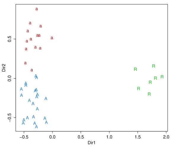
Figure 1: Projection of coffee data samples marked according to the clustering obtained from the variables selected using the forward/backward greedy search. The symbol R indicates Robusta coffees, A and a the sub-varieties of Arabica coffees.

4.4 Simulated high-dimensional data

Witten and Tibshirani (2010, Sec. 3.3.2) discussed an example where five clustering variables are conditionally independent given the cluster memberships, whereas the remaining twenty features are simply independent standard normal variables, also independent from the clustering ones. The first five variables are distributed according to a spherical Gaussian distribution with mean $\boldsymbol{\mu}_{1}=(\mu,\mu,\ldots,\mu)$, $\boldsymbol{\mu}_{2}=\boldsymbol{0}$, $\boldsymbol{\mu}_{3}=-\boldsymbol{\mu}_{1}$, where $\mu=1.7$, and common unit standard deviation. We replicated this experiment (denoted by WT) with varying sample sizes ($n_{g}$ cases for each group) and for a set of different techniques.

Table 3 reports the variable selection error rate (VSER) and the classification error rate (CER). As already mentioned in Section 4.1, the VSER is defined as the ratio of the number of errors in selecting (or not selecting) variables with respect to the total number of variables considered. The CER between two partitions, which is equivalent to one minus the Rand index (Rand, 1971), is equal to 0 in the case of perfect agreement, and becomes larger for increasing disagreement (for a formal definition see Witten and Tibshirani, 2010). Smaller values of both VSER and CER are better. These two measures have been chosen for the purpose of comparison with the results in Witten and Tibshirani (2010, Tab. 4) and Celeux et al. (2013, Sect. 3.1).

The model with uniformly better performance is the MCLUST model with the first five variables, i.e. the model which most resembles the data generation mechanism. However, this model is not available when we do not know the clustering variables, as we are assuming here. SPARSEKMEANS performs well in term of accuracy, but the number of selected variables increases with group sample size, and all the features are selected for $n_{g}=50$. MCLUST using all the variables and EII parameterisation, both at the hierarchical initialisation step and for the mixture modelling, has quite good accuracy and improves as group sample size increases. CLUSTVARSEL using backward/forward greedy search, with EII parameterisation both for modelling and initialisation also has good accuracy, and improves as group sample size gets larger. For $n_{g}=50$ it is equivalent to the best models. However, the VSER is better than for the other methods, and improves as $n_{g}$ gets larger. Thus, for increasing sample size it converges to the true subset size. Note that forward/backward greedy search is clearly less accurate than the backward/forward search, with the VSER which is also larger, so the performance is overall worst than that of backward/forward search. Finally, results for CLUSTVARSEL using backward/forward greedy search are essentially equivalent to those obtained with the SELVARCLUSTINDEP software of Maugis et al. (2009b).

Table 3: Average values based on 100 simulation runs for the WT simulation scheme with group sample size $n_{g}$. All models assume the number of clusters $G=3$ to be known. For all the MCLUST models, including those fitted by the variables subset selection algorithm, the EII parameterisation was used for both the hierarchical initialization and the mixture modeling. CLUSTVARSEL[fwd] uses the forward/backward greedy search, whereas CLUSTVARSEL[bkw] uses the backward/forward greedy search. Smaller values of both VSER and CER are better.

	VSER				CER
Model	$n_{g}=10$	$n_{g}=20$	$n_{g}=50$		$n_{g}=10$	$n_{g}=20$	$n_{g}=50$
K-MEANS	.800	.800	.800		.258	.248	.224
SPARSEKMEANS	.438	.678	.800		.070	.066	.055
MCLUST[$X_{1},\ldots,X_{5}$]	.000	.000	.000		.063	.064	.054
MCLUST[$X_{1},\ldots,X_{25}$]	.800	.800	.800		.129	.093	.060
CLUSTVARSEL[fwd]	.268	.200	.054		.370	.275	.090
CLUSTVARSEL[bkw]	.180	.081	.033		.151	.082	.053
SELVARCLUSTINDEP	.216	.098	.032		.162	.089	.057
Standard errors are all $<.030$.

5 Adjustments for speeding up the algorithm

5.1 Sub-sampling at hierarchical initialisation step

The EM algorithm is initialised in mclust using the partitions obtained from model-based agglomerative hierarchical clustering. Efficient numerical algorithms for approximately maximizing the classification likelihood with multivariate normal models have been discussed by Fraley (1998). However, for datasets having a large number of observations this step can be computationally expensive.

When the number of observations is large, we may allow clustvarsel to use only a subset of the observations at the model-based hierarchical stage of clustering, to speed up the algorithm. This is easily done by setting the argument samp = TRUE, and by specifying the number of observations to be used in the hierarchical clustering subset with sampsize.

Consider the following simulation scheme which constructs a medium sized dataset on five dimensions. Only the first two variables contain clustering information, the third is highly correlated with the first one, whereas the remaining features are simply noise variables.

R> library(MASS)R> n = 1000     # sample sizeR> pro = 0.5    # mixing proportionR> mu1 = c(0,0) # mean vector for the first clusterR> mu2 = c(3,3) # mean vector for the second clusterR> sigma1 = matrix(c(1,0.5,0.5,1),2,2)       # covar matrix for the first clusterR> sigma2 = matrix(c(1.5,-0.7,-0.7,1.5),2,2) # covar matrix for the second clusterR> X = matrix(0, n, 5); colnames(X) = paste("X", 1:ncol(X), sep ="")R> # generate the clustering variablesR> set.seed(123)R> u = runif(n)R> Class = ifelse(u < pro, 1, 2)R> X[u < pro, 1:2]  = mvrnorm(sum(u < pro), mu = mu1, Sigma = sigma1)R> X[u >= pro, 1:2] = mvrnorm(sum(u >= pro), mu = mu2, Sigma = sigma2)R> # generate the non-clustering variablesR> X[,3] = X[,1] + rnorm(n)R> X[,4] = rnorm(n, mean = 1.5, sd = 2)R> X[,5] = rnorm(n, mean = 2, sd = 1)R> clPairs(X, Class, gap = 0.2)

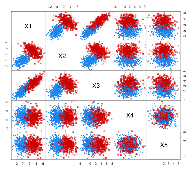
Figure 2: Scatterplot matrix of simulated data with points marked according to the known groups.

We may compare the procedure which uses sampling at the hierarchical stage with the default call to clustvarsel, both in term of computing time, using the function system.time, and in term of clustering accuracy.

R> system.time(result1 <- clustvarsel(X, G = 1:5, samp = TRUE, sampsize = 200))

   user  system elapsed  6.033   0.009   6.044

R> system.time(result2 <- clustvarsel(X, G = 1:5))

   user  system elapsed  9.739   0.044   9.820

Thus, by using sub-sampling for the initial hierarchical clustering we get an algorithm that is 38% faster with the same accuracy:

R> result1$subset

X2 X1 2  1

R> result2$subset

X2 X1 2  1

To investigate the effect of sampling as the number of observations increase we conducted a small simulation study by replicating the above simulation setting with different sample sizes and fixed size at 200 observations for choosing the initial starting points. Figure 3 shows the results averaged over 10 replications. Panel (a) reports the computing time required as the sample size grows, whereas panel (b) shows the relative gain from using a subset of observations at the initial hierarchical stage. As can be seen, efficiency improves roughly exponentially as the number of observations increases, with sampling being about 40 times faster at $10,000$ cases. As the system time required increases linearly for sampling, when no sampling is used at the initial stage the time required increases approximately exponentially. Furthermore, in all the replications the first two variables have been selected by both methods. Hence, the improvement in terms of computational efficiency has not caused any deterioration in terms of accuracy.

(a)

(b)

Figure 3: Comparison of computing time vs sample size. Panel (a) shows the average over 10 replications for clustvarsel using sub-sampling with fixed size at 200 observations, and no sampling. Panel (b) shows the relative gain of sub-sampling, calculated as the ratio of system times for no sampling and sub-sampling. All axes are on the logarithmic scale.

5.2 Headlong search

When a dataset contains a large number of variables we may find that using the headlong search algorithm option (search = "headlong") is faster than the default greedy search. To show an example we simulated a dataset analogous to the previous one for the clustering variables, then six more irrelevant variables were added, some correlated with the clustering ones, some independent and some correlated among themselves. Then, we may compare the time required by using the headlong method and using the greedy method.

R> library(MASS)R> n = 400      # sample sizeR> pro = 0.5    # mixing proportionR> mu1 = c(0,0) # mean vector for the first clusterR> mu2 = c(3,3) # mean vector for the second clusterR> sigma1 = matrix(c(1,0.5,0.5,1),2,2)       # covar matrix for the first clusterR> sigma2 = matrix(c(1.5,-0.7,-0.7,1.5),2,2) # covar matrix for the second clusterR> X = matrix(0, n, 10); colnames(X) = paste("X", 1:ncol(X), sep ="")R> # generate the clustering variablesR> set.seed(1234)R> u = runif(n)R> Class = ifelse(u < pro, 1, 2)R> X[u < pro, 1:2]  = mvrnorm(sum(u < pro), mu = mu1, Sigma = sigma1)R> X[u >= pro, 1:2] = mvrnorm(sum(u >= pro), mu = mu2, Sigma = sigma2)R> # generate the non-clustering variablesR> X[,3] = X[,1] + rnorm(n)R> X[,4] = X[,2] + rnorm(n)R> X[,5] = rnorm(n, mean = 1.5, sd = 2)R> X[,6] = rnorm(n, mean = 2, sd = 1)R> X[,7:8] = mvrnorm(n, mu = mu1, Sigma = sigma1)R> X[,9:10] = mvrnorm(n, mu = mu2, Sigma = sigma2)

R> system.time(result1 <- clustvarsel(X, G = 1:5, search = "headlong"))

   user  system elapsed  5.818   0.029   5.847

R> system.time(result2 <- clustvarsel(X, G = 1:5))

   user  system elapsed 10.107   0.033  10.139

In situations where there are many observations and a large number of variables, sub-sampling at the hierarchical initialisation step and the headlong search can be used concurrently to improve computational efficiency. A small simulation study was conducted by replicating the previous simulation scheme with different sample sizes. The methods compared are greedy and headlong searches, without and with sampling using sampize = 200. The results averaged over 10 replications are shown in Figure 4. Without sampling, headlong search is faster than greedy search with a constant relative gain of about $1.7$. The use of sampling at the initial hierarchical stage enables us to achieve an exponential relative gain as the sample size increases for both type of searches. Also in this case, the headlong search appears to be about twice as fast as the greedy search.

(a)

(b)

Figure 4: Comparison of computing time vs sample size. Panel (a) shows the average over 10 replications for clustvarsel using search = "greedy" with and without sampling, and search = "headlong" with and without sampling. A fixed value sampsize = 200 is used throughout. Panel (b) shows the relative gain, calculated as the ratio of system times, of each strategy against the default greedy search with no sampling. All axes are on the logarithmic scale.

The speed/optimally tradeoff in a headlong search can be changed by increasing or decreasing the different levels, e.g. by setting the upper level to 10 instead of 0 we would require a variable to have stronger evidence of clustering before it is included, and by setting the lower level to 0 we would remove variables that at any stage have evidence of clustering weaker by any amount than evidence against clustering.

5.3 Parallel computing

Parallel computing is a form of computation in which the required calculations are performed simultaneously, either on a single multi-core processors machine or on a cluster of multiple computers.

Direct support of parallelism in R is available since version 2.14.0 (released in October 2011) through the package parallel (R Core Team, 2014). This is essentially a merger of the multicore package (Urbanek, 2011) and the snow package (Tierney et al., 2013). The multicore functionality supports parallelism via forking, which is a concept from POSIX operating systems, so it is available on all R platforms except Windows. In contrast, snow supports different transport mechanisms (e.g. socket connections) to communicate between the master and the workers, and it is available on all operating systems. Other approaches to parallel computing in R are available as described in McCallum and Weston (2011). For an extensive list of packages see CRAN task view on High-Performance and Parallel Computing with R at http://cran.r-project.org/web/views/HighPerformanceComputing.html.

The greedy search discussed in Section 2 constitutes an embarrassingly parallel problem, i.e. one for which little or no effort is required to separate the problem into a number of parallel tasks. Essentially, the sequential evaluation of candidate variables for inclusion or exclusion, which is the most time consuming task, can be done in parallel. For the actual implementation in clustvarsel we used the doParallel package (Revolution Analytics and Weston, 2013a), a “parallel backend” which acts as an interface between the foreach package (Revolution Analytics and Weston, 2013b) and the parallel package. Essentially, it provides a mechanism needed to execute for loops in parallel.

To specify if parallel computing should be used in the evaluation of the $\text{BIC}_{\text{diff}}$ criterion in (1), the optional argument parallel must be set to TRUE in the clustvarsel function call. In this case all the available cores, as returned by the detectCores function, are used. A numeric value specifying the number of cores to employ can also be specified in the optional argument parallel. Finally, the parallelisation functionality depends on system OS: on Windows only ’snow’ type functionality is available, whereas on Unix/Linux/Mac OSX both ’snow’ and ’multicore’ (default) functionalities are available.

As an example, consider a sample of $n=200$ observations generated according to the simulation scheme described in Section 5.2. We may compare the sequential greedy backward/forward search with a parallel version of the algorithm with the default maximum cores available and by specifying 2 cores (on a MacBook Pro with i5 Intel^® CPU with 4 cores running at $2.3$GHz and with $4$GB of RAM):

R> system.time(result1 <- clustvarsel(X, G = 1:9, direction = "backward"))

   user  system elapsed103.860   0.509 104.774

R> system.time(result2 <- clustvarsel(X, G = 1:9, direction = "backward",                                      parallel = TRUE))

   user  system elapsed158.578   5.685  51.254

R> system.time(result2 <- clustvarsel(X, G = 1:9, direction = "backward",                                      parallel = 2))

   user  system elapsed119.161   2.887  67.221

In this case, by using 4 cores we were able to halve the computing time, whereas a 35% speed up is achieved using 2 cores.

By using a machine with $P$ processors instead of just one, we would like to obtain an increase in calculation speed of $P$ times. As shown above, this is not the case because in the implementation of a parallel algorithm there are some inherent non-parallelizable parts and communication costs between tasks (Nakano, 2012). Amdahl’s Law (Amdahl, 1967) is often used in parallel computing to predict the theoretical maximum speedup when using multiple processors. If $f$ is the fraction of non-parallelizable task and $P$ is the number of processors in use, then the maximum speedup achievable on a parallel computing platform is given by

$$S_{P}=\frac{1}{f+(1-f)/P}.$$ (3)

In the limit, the above ratio converges to $S_{\max}=1/f$, which represents the maximum increase of speed achievable in theory, i.e. by a machine with an infinite number of processors.

To investigate the performance of our parallel algorithm implementation, we conducted a small simulation study using the above simulation setting for increasing numbers of cores. The study was performed on a 24 cores Intel^® Xeon^® CPU X5675 running at $3.07$GHz and with $128$GB of RAM. Figure 5 shows the results averaged over 10 replications. The points represent the observed speedup factor (obtained as $s_{P}=t_{1}/t_{P}$, where $t_{P}$ is the system time employed using $P$ cores) for running the backward algorithm with up to 10 cores. The curve represents the Amdahl’s Law (3) with $f$ estimated by non-linear least squares. It turns out that the estimated fraction of sequential part of the backward/forward search for variable selection is $\hat{f}=0.13$, which yields a maximum speedup of $S_{\max}=7.7$.

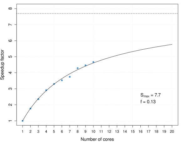
Figure 5: Graph of speedup factor vs the number of cores employed in the parallel algorithm for backward/forward subset selection in model-based clustering. The estimated fraction of non-parallelizable task is estimated as $f=0.13$, which gives a maximum speedup achievable by parallelisation of around $7.7$ times the sequential algorithm.

6 Conclusions and future work

This paper has presented the R package clustvarsel which provides a convenient set of tools for variable selection in model-based clustering using a finite mixture of Gaussian densities. Stepwise greedy search and headlong algorithm are implemented in order to find the (locally) optimal subset of variables with cluster information. The computational burden of such algorithms can be decreased by some ad hoc modifications in the algorithms, or via the use of parallel computation as implemented in the package. Examples illustrating the use of the package in practical applications have been presented. Finally, given the vast solution space, other optimisation techniques could be usefully employed. For instance, the use of genetic algorithms as described in Scrucca (2014) will be included in a future release of the package.

References

- (1)
- Amdahl (1967) Amdahl GM (1967). “Validity of the single processor approach to achieving large scale computing capabilities.” In AFIPS Conference Proceedings, volume 30, pp. 483–485.
- Analytics (2012) Analytics R (2012). iterators: Iterator construct for R. R package version 1.0.6, URL \urlhttp://CRAN.R-project.org/package=iterators.
- Badsberg (1992) Badsberg JH (1992). “Model Search in Contingency tables by CoCo.” In Y Dodge, J Whittaker (eds.), Computational Statistics, volume 1, pp. 251–256.
- Banfield and Raftery (1993) Banfield JD, Raftery AE (1993). “Model-based Gaussian and non-Gaussian clustering.” Biometrics, 48, 803–821.
- Campbell and Mahon (1974) Campbell N, Mahon R (1974). “A multivariate study of variation in two species of rock crab of genus Leptograpsus.” Australian Journal of Zoology, 22, 417–425.
- Celeux and Govaert (1995) Celeux G, Govaert G (1995). “Gaussian Parsimonious Clustering Models.” Pattern Recognition, 28(5), 781–793.
- Celeux et al. (2013) Celeux G, Martin-Magniette ML, Maugis-Rabusseau C, Raftery AE (2013). “Comparing Model Selection and Regularization Approaches to Variable Selection in Model-Based Clustering.” ArXiv e-prints. \url1307.7860.
- Fraley (1998) Fraley C (1998). “Algorithms for model-based Gaussian hierarchical clustering.” SIAM Journal on Scientific Computing, 20(1), 270–281.
- Fraley et al. (2014) Fraley C, Raftery A, Scrucca L (2014). mclust: Normal Mixture Modeling for Model-Based Clustering, Classification, and Density Estimation. R package version 4.3, URL \urlhttp://CRAN.R-project.org/package=mclust.
- Fraley and Raftery (2002) Fraley C, Raftery AE (2002). “Model-Based Clustering, Discriminant Analysis, and Density Estimation.” Journal of the American Statistical Association, 97, 611–631.
- Fraley et al. (2012) Fraley C, Raftery AE, Murphy TB, Scrucca L (2012). MCLUST Version 4 for R: Normal Mixture Modeling for Model-Based Clustering, Classification, and Density Estimation.
- Hubert and Arabie (1985) Hubert L, Arabie P (1985). “Comparing partitions.” Journal of Classification, 2, 193–218.
- Maugis et al. (2009a) Maugis C, Celeux G, Martin-Magniette M (2009a). “Variable Selection for Clustering with Gaussian Mixture Models.” Biometrics, 65(3), 701–709.
- Maugis et al. (2009b) Maugis C, Celeux G, Martin-Magniette M (2009b). “Variable selection in model-based clustering: A general variable role modeling.” Computational Statistics & Data Analysis, 53(11), 3872–3882.
- McCallum and Weston (2011) McCallum E, Weston S (2011). Parallel R. O’Reilly Media.
- McLachlan and Peel (2000) McLachlan GJ, Peel D (2000). Finite Mixture Models. Wiley, New York.
- Miller (1990) Miller AJ (1990). Subset Selection in Regression. Number 40 in Monographs on Statistics and Applied Probability. Chapman and Hall.
- Nakano (2012) Nakano J (2012). “Parallel computing techniques.” In JE Gentle, WK Härdle, Y Mori (eds.), Handbook of Computational Statistics, 2nd ed. edition, pp. 243–271. Springer.
- R Core Team (2014) R Core Team (2014). R: A Language and Environment for Statistical Computing. R Foundation for Statistical Computing, Vienna, Austria. URL \urlhttp://www.R-project.org/.
- Raftery et al. (2013) Raftery A, Hoeting J, Volinsky C, Painter I, Yeung KY (2013). BMA: Bayesian Model Averaging. R package version 3.16.2.3, URL \urlhttp://CRAN.R-project.org/package=BMA.
- Raftery and Dean (2006) Raftery AE, Dean N (2006). “Variable Selection for Model-Based Clustering.” Journal of the American Statistical Association, 101(473), 168–178.
- Rand (1971) Rand W (1971). “Objective criteria for the evaluation of clustering methods.” Journal of the American Statistical Association, 66(336), 846–850.
- Revolution Analytics and Weston (2013a) Revolution Analytics, Weston S (2013a). doParallel: Foreach parallel adaptor for the parallel package. R package version 1.0.6, URL \urlhttp://CRAN.R-project.org/package=doParallel.
- Revolution Analytics and Weston (2013b) Revolution Analytics, Weston S (2013b). foreach: Foreach looping construct for R. R package version 1.4.1, URL \urlhttp://CRAN.R-project.org/package=foreach.
- Scrucca (2010) Scrucca L (2010). “Dimension reduction for model-based clustering.” Statistics and Computing, 20(4), 471–484. \hrefhttp://dx.doi.org/10.1007/s11222-009-9138-7doi:10.1007/s11222-009-9138-7.
- Scrucca (2014) Scrucca L (2014). “Genetic Algorithms for Subset Selection in Model-Based Clustering.” Unpublished manuscript.
- Streuli (1973) Streuli H (1973). “Der heutige stand der kaffeechemie.” In Association Scientifique International du Cafe, 6th International Colloquium on Coffee Chemisrty, pp. 61–72. Bogata, Columbia.
- Tierney et al. (2013) Tierney L, Rossini AJ, Li N, Sevcikova H (2013). snow: Simple Network of Workstations. R package version 0.3-13, URL \urlhttp://CRAN.R-project.org/package=snow.
- Urbanek (2011) Urbanek S (2011). multicore: Parallel processing of R code on machines with multiple cores or CPUs. R package version 0.1-7, URL \urlhttp://CRAN.R-project.org/package=multicore.