Quantum Uncertainty and Error-Disturbance Tradeoff

Abstract

The uncertainty principle is often interpreted by the tradeoff between the error of a measurement and the consequential disturbance to the followed ones, which originated long ago from Heisenberg himself but now falls into reexamination and even heated debate. Here we show that the tradeoff is switched on or off by the quantum uncertainties of two involved non-commuting observables: if one is more certain than the other, there is no tradeoff; otherwise, they do have tradeoff and the Jensen-Shannon divergence gives it a good characterization.

Uncertainty is an intrinsic feature of quantum mechanics that individual particles could have no certain values with respect to a quantum observable. A famous example is Schrödinger’s cat which stays in a superposition of both alive and dead rather than either. Although nearly one hundred years have passed since the dawn of quantum theory, new discovers behind quantum uncertainty are still underway. Recent work has illuminated quantum uncertainty’s relations to quantum non-locality uncertainty-nonlocality , nonclassical correlations correlation , thermodynamics second law and so on. For the general public, quantum uncertainty becomes well-known because of Heisenberg’s uncertainty principle heisenberg accompanied by the inequality $\sigma_{x}\sigma_{p}\geq\hbar/2$ ($\sigma$ is the standard deviation). The principle is also embodied in Robertson’s inequality $\sigma_{A}\sigma_{B}\geq\frac{1}{2}|\langle\psi|[A,B]|\psi\rangle|^{2}$ robertson and Maassen-Uffink’s entropic inequality $H_{\rho}(A)+H_{\rho}(B)\geq-2\mathrm{ln}c_{AB}$ entropy ; entropy relation . Here $c_{AB}=\mathrm{max}_{ij}|\langle a_{i}|b_{j}\rangle|$, where $\{|a_{i}\rangle\}$ and $\{|b_{j}\rangle\}$ are the eigenstates of two observables $A$ and $B$, respectively, and $H_{\rho}(A)$ is the Shannon entropy of the outcome distribution generated in the ideal measurements of $A$ on ensemble $\rho$, which is determined theoretically by Born’s rule.

Following the presentation of Heisenberg himself heisenberg , the uncertainty principle is often interpreted in textbooks feynman as a consequence of the tradeoff: the higher the resolution (precision) of measuring position is, the stronger the disturbance to particle’s momentum will be. The heart of such an interpretation positions at the back-action of quantum measurements, as Dirac wrote “a measurement always causes the system to jump into an eigenstate of the dynamical variable that is being measured $\cdots$” dirca . However, these famous inequalities mentioned above do not necessarily cover the effect of back-action and thus the relation between precision and disturbance. To experimentally test these inequalities, one could prepare two identical ensembles and measures the observables separately rather than sequentially. In order to settle such a discrepancy and give a rigorous analysis to the tradeoff relation in the mind of Heisenberg, Ozawa firstly considered a measurement of observable $A$ occurred between the system in state $|\psi\rangle$ and the measurement device (the “meter”) in state $|\xi\rangle$. As a result, he derived an inequality ozawa which has been verified extensively in experiments weak measurement ; neutron ; other1 ; other2 ; minima ; weak2 :

$$\epsilon_{A}\eta_{B}+\epsilon_{A}\sigma_{B}+\eta_{B}\sigma_{A}\geq\frac{1}{2}|\langle\psi|[A,B]|\psi\rangle|.$$ (1)

Here the error of this measurement is defined as $\epsilon_{A}^{2}=\langle\psi,\xi|(U^{\dagger}(I\otimes M)U-A\otimes I)^{2}|\psi,\xi\rangle$, where the meter observable is $M$, $U$ is the coupling unitary, and $I$ is the identity operator. The consequential disturbance to the system about observable $B$ is defined as $\eta_{B}^{2}=\langle\psi,\xi|(U^{\dagger}B\otimes IU-B\otimes I)^{2}|\psi,\xi\rangle$.

Recently this relation triggered a heated debate proposition ; qubitwenner ; arxives ; defi-discussion ; penas ; other3 ; buschproof ; rudolph ; entropic independ . The controversial issue is what definition can exactly represent the physical concepts of error and disturbance. The authors of Ref. rudolph proposed an operational criterion which requires (1) error to be nonzero if the outcome distribution produced in an actual measurement of $A$ deviates from that predicted by Born’s rule, and (2) disturbance to be nonzero if the back-action introduced by the actual measurement alters the original distribution with respect to $B$. $\epsilon_{A}$ and $\eta_{B}$ defined by Ozawa are criticized since they violate the above two requirements. Following the requirements, the authors have showed in Ref. rudolph that $\langle\psi|[A,B]|\psi\rangle$ and $c_{AB}$, two characters of uncertainty principle, are excluded to appear alone on the right hand side of inequalities in the form of Eq. (1), leaving an open problem as what can be there. Furthermore, Ozawa’s inequality does depend on the magnitudes of eigenvalues. But eigenvalues are not essential to non-commuting observables and what really crucial is the family of eigenstates. This motivates the information-theoretical approaches (like the entropic uncertainty relation entropy ; entropy relation ) that do not depend on eigenvalues. Meanwhile, some authors reported state-independent theories qubitwenner ; buschproof ; entropic independ where the scenarios behave like benchmarking machines that just get off the production line. The details relevant to various input states are erased in the construction of inequalities qubitwenner ; buschproof or have never been taken into account entropic independ .

In spite of the intricate features, we notice the presence of $\sigma_{A}$, $\sigma_{B}$ in Eq. (1), and the Shannon entropy $H_{\rho}(B)$ in the inequality proposed in Ref. other3 . It inspires us to consider the relevance of quantum uncertainty in state-dependent context. Does quantum uncertainty play some intrinsic role behind? Consisting on operational definitions satisfying the requirements proposed in Ref. rudolph , we will show that the tradeoff between error and disturbance is switched off or on according to the quantum uncertainties (or certainties) of the outcome distributions of measuring $A$ and $B$. When it is switched on, via a generally valid strategy, an inequality will be constructed to bound their tradeoff from below.

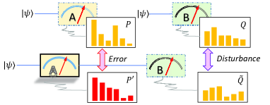
Figure 1: Error and Disturbance. Dashed boxes and yellow-color bar charts stand for the ideal measurements of which the results is determined by Born’s rule. The solid box stands for the real-life apparatus which produces the red-color distribution $P^{\prime}$. The difference between $P$ and $P^{\prime}$ is caused by the imperfection of the apparatus, and the difference between $Q$ and $\tilde{Q}$ is caused by the inevitable back-action brought by the apparatus. Thus we define the error $Err_{\psi}(A)$ and the disturbance $Dis_{\psi}(B)$ as in Eq. (2).

Error and disturbance. Let us focus on the scenario illustrated in Fig. 1. By the logic of quantum mechanics, the complete description of an isolated system is a state vector $|\psi\rangle$ in a Hilbert space dirca ; von , and what we obtain from quantum measurement is a statistical distribution of different outcomes with respect to the measured observable, as determined theoretically by Born’s rule. Suppose that Born’s rule gives the distributions $P=\{p_{1},p_{2}\cdots p_{d}\}$ and $Q=\{q_{1},q_{2}\cdots q_{d}\}$, respectively, to the measurements of observables $A$ and $B$ on $|\psi\rangle$. Then consider a real-life measurement of $A$ performed on $|\psi\rangle$, during which the employed real-life apparatus (together with the inevitable environment) select a preferred pointer basis in system’s Hilbert space zurek . As a result, the entire state evolves to be $\sum_{i}^{d}\sqrt{p^{\prime}_{i}}|a^{\prime}_{i}\rangle_{s}|\phi_{i}\rangle_{a}$, where indexes s and a label the system and the apparatus (possibly including the environment), and $\langle a^{\prime}_{i}|a^{\prime}_{j}\rangle=\langle\phi_{i}|\phi_{j}\rangle=\delta_{ij}$. The apparatus bridges the quantum system and the classical world we stay in. It returns an outcome from the set ${1,2,\cdots d}$ and finally generates the distribution $P^{\prime}=\{p_{1}^{\prime},p_{2}^{\prime}\cdots p_{d}^{\prime}\}$ with $p^{\prime}_{i}=|\langle\psi|a^{\prime}_{i}\rangle|^{2}$. Statistically, the quantum system is then mapped to $\rho=\sum_{i}p^{\prime}_{i}|a^{\prime}_{i}\rangle\langle a^{\prime}_{i}|$. So the error comes from the deviation between $\{|a^{\prime}_{i}\rangle\}_{i}$ and $\{|a_{i}\rangle\}_{i}$ caused by maybe the misalignment of devices. To quantify the error of such a real-life measurement of $A$, we have to compare the information at hand, $P^{\prime}$, to the ideal one predicted by Born’s rule. Thus, we define the error, $Err_{\psi}(A)$, to be specified below, to quantify the difference between $P$ and $P^{\prime}$.

Here the modeled real-life measurements are projective measurements that are maximally informative maximally informative . We do not consider the more general positive-operator valued measurements (POVM) because fundamentally speaking, they are projective measurements performed on a larger quantum system.

The disturbance caused by the back-action of the real-life measurement of $A$ is embodied in the inequivalence between $|\psi\rangle$ and $\rho$. With respect to observable $B$, the disturbance displays as the difference between the distribution $Q$ and $\tilde{Q}=\{\tilde{q}_{j}=\langle b_{j}|\rho|b_{j}\rangle\}_{j=1}^{d}$, both of which are determined by Born’s rule. If $\tilde{Q}=Q$, the induced disturbance to $B$ cannot be perceived. So we define the disturbance term by the divergence between $\tilde{Q}$ and $Q$.

Being based on the above observation, any distance function $D(\cdot,\cdot)$ that vanishes if and only if the two distributions are identical, such as the relative entropy $D(P||P^{\prime})=\sum_{m}p_{m}\mathrm{ln}(p_{m}/p_{m}^{\prime})$, can serve as a quantification of error and disturbance. Explicitly, we quantify the error and the disturbance $Dis_{\psi}(B)$ as

$$Err_{\psi}(A)=D_{1}(P,P^{\prime}),\;\;Dis_{\psi}(B)=D_{2}(Q,\tilde{Q}),$$ (2)

where the indices “1” and “2” mean that the two $D$-functions are not necessary to be identical. These definitions obey the basic operational requirements proposed in Ref. rudolph . After the above preparation, let us present one of our main results.

Theorem-1. For any $d$-dimensional pure state $|\psi\rangle$, there exists projective measurements such that $Err_{\psi}(A)$ and $Dis_{\psi}(B)$ vanish simultaneously if and only if $P\succ Q$, i.e., there is no tradeoff between the error of measuring $A$ and the consequential disturbance to $B$. $\blacksquare$

“$P\succ Q$”, read $P$ majorizes $Q$, means if sorting the elements from larger to smaller, i.e., $p_{1}\geq p_{2}\geq\cdots p_{d}$ and $q_{1}\geq q_{2}\geq\cdots q_{d}$, then $\sum_{i=1}^{k}p_{i}\geq\sum_{i=1}^{k}q_{i}$ for $k=1,2\cdots d$ majorization . To give an impression, the probability distribution of an event with certainty is in form of $(1,0,0\cdots 0)$, which majorizes all the other distributions; the uniform distribution $(\frac{1}{d},\frac{1}{d}\cdots\frac{1}{d})$ that belongs to the most uncertain events, is majorized by all the others. By definition, $P\succ Q$ means the occurrence probability of a top-$k$ high-probability outcome in the ideal measurement of $A$ is no less than that of $B$, for all possible values of $k$. Thus, majorization gives a rigorous criterion for the partial order of certainty or uncertainty. Moreover, $P\succ Q$ leads to $H(P)\leq H(Q)$, as widely accepted that larger Shannon entropy means more uncertainty. So Theorem-1 concludes that if the outcomes of measuring $A$ is more certain, we are able to obtain the correct distribution of $A$ by a projective measurement without disturbing the distribution of $B$. This result takes a giant stride forward from the extreme case when $|\psi\rangle$ is an eigenstate of $A$ thus $P=\{0\cdots,1,0,\dots 0\}$ and must majorize $Q$. We leave the technic proof of Theorem-1 in the Supplemental Material.

It is interesting to compare Theorem-1 with Ref. rudolph where the authors proved the existence of $2^{d-1}$ zero-noise (zero-error) and zero-disturbance states (ZNZD) for sequential ideal measurements of $A$ and $B$. The conclusion of Theorem-1 looks resemblant to it at the first glance. However, the two are based on different perspectives. Here we define error from probability distributions without considering posterior states because we cannot distinguish $|a^{\prime}_{i}\rangle$ from $|a_{i}\rangle$, with only the real-life apparatus at hand. For fixed $A$ and $B$, Theorem-1 identifies a set of states upon which $P\succ Q$. As a subset of system’s Hilbert space, it has a non-zero measure. Although the measure of the discrete set of the $2^{d-1}$ states is zero, the ZNZD states are defined for ideal measurements of $A$ instead of those performed with real-life apparatus. Thus the ZNZD states can be valid for errors quantified more strictly than ours. Additionally, maybe a coincidence, the proof of Theorem-1 supplies an algorithm to find generally also $2^{d-1}$ different realizations of $\{|a^{\prime}_{i}\rangle\}_{i}$ upon which $Err_{\psi}(A)$ and $Dis_{\psi}(B)$ are null simultaneously.

Next, if $P\nsucc Q$, $Err_{\psi}(A)+Dis_{\psi}(B)$ must have a positive lower bound. To find it, we treat the sum as a functional of the probability distribution pair $(P^{\prime},\tilde{Q})$. As coordinates, all pairs $(P^{\prime},\tilde{Q})=(p_{1}^{\prime},\cdots p_{d}^{\prime},\tilde{q}_{1}\cdots\tilde{q}_{d})$ compose a $2(d-1)$-dimensional sub-manifold $\mathcal{S}_{0}$ of the $2d$-dimensional Euclid space, due to the restrictions that $\sum_{i}p_{i}^{\prime}=1$ and $\sum_{i}\tilde{q}_{i}=1$. Meanwhile, the exact bound of $Err_{\psi}(A)+Dis_{\psi}(B)$ is the minima over a subset of $\mathcal{S}_{0}$ defined by $p_{i}^{\prime}=|\langle a_{i}^{\prime}|\psi\rangle|^{2}$ and $\tilde{q}_{j}=\sum_{i}p_{i}^{\prime}|\langle a_{i}^{\prime}|b_{j}\rangle|^{2}$ (ranging over all orthogonal basis $\{|a_{i}^{\prime}\rangle\}$), which we call $\mathcal{S}_{2}.$ Looking at the problem in $\mathcal{S}_{0}$, the target is to find the point in $\mathcal{S}_{2}$ which is the closest to $(P,Q)\notin\mathcal{S}_{2}$, where “closest” is defined by the $D$-functions applied in Eq. (2). Analytical solution of the exact bound seems complicated to approach and must shape terrible because of the involved geometry of $\mathcal{S}_{2}$ when embedded in $\mathcal{S}_{0}$ (see Fig. 2).

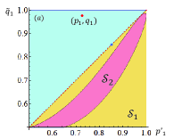
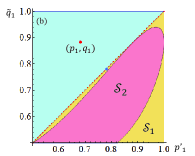
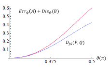
Figure 2: Imbedding $\mathcal{S}_{2}$ and $\mathcal{S}_{1}$ in $\mathcal{S}_{0}$ when $d=2$. $\mathcal{S}_{0}$ is parameterized by $(p^{\prime}_{1},\tilde{q}_{1})$ and thus illustrated by the $[0,1]\times[0,1]$ square. We fix the labeling of eigenstates of $A$ and $B$ such that $p_{1}\geq p_{2}$ and $q_{1}\geq q_{2}$. The pink-shape region is $\mathcal{S}_{2}$, a subset of $\mathcal{S}_{1}$ filled with yellow. When $D$-functions in Eq. (2) are the relative entropy, it is sufficient to consider only the component where $p^{\prime}_{1}\geq p^{\prime}_{2}$ and $\tilde{q}_{1}\geq\tilde{q}_{2}$. $(a),(b)$ show the details of that component when $P\nsucc Q$ and $(p_{1},q_{1})$ equals to $(0.727,0.978)$ and $(0.681,0.882)$, respectively. The right hand side of Eq. (4) is obtained on the blue points, which locate on the surface of $\mathcal{S}_{1}$. The line-chart illustrates the exact lower bound (red) of $Err_{\psi}(A)+Dis_{\psi}(B)$ and lower bound $D_{JS}(P,Q)$ (blue) determined by Theorem-2, when $A=\sigma_{z}$, $B=\sigma_{x}$, and $|\psi(\theta)\rangle=\cos(\theta/2)|0\rangle+\sin(\theta/2)|1\rangle$ with $\theta\in[\pi/4,\pi/2]$ such that $Q\succ P$. Here, $\sigma_{z}|0\rangle=|0\rangle$ and $\sigma_{z}|1\rangle=-|1\rangle$.

However, we can extend $D_{1}(P,P^{\prime})+D_{2}(Q,\tilde{Q})$ naturally from $\mathcal{S}_{2}$ to the entire $\mathcal{S}_{0}$. Define the set of pairs satisfying $P^{\prime}\succ\tilde{Q}$ as $\mathcal{S}_{1}$. According to Horn’s theorem majorization which says two distributions $P^{\prime}\succ\tilde{Q}$ if and only if there is a unitary $U$ such that $p_{i}^{\prime}=\sum_{j}|U_{ij}|^{2}\tilde{q}_{j}$, $\mathcal{S}_{2}$ must be a subset of $\mathcal{S}_{1}$. Thus we have $\mathcal{S}_{2}\subset\mathcal{S}_{1}\subset\mathcal{S}_{0}$ and $\mathrm{min}_{\mathcal{S}_{2}}(\cdots)\geq\mathrm{min}_{\mathcal{S}_{1}}(\cdots)$ by logic. Moreover, enormous $D$-functions make the point $(P,Q)\notin\mathcal{S}_{1}$ be the unique extreme point of $Err_{\psi}(A)+Dis_{\psi}(B)$ in $\mathcal{S}_{0}$ such that its minima value over $\mathcal{S}_{1}$ must be obtained at the surface of $\mathcal{S}_{1}$. This surface consists of many faces, especially those defined by majorization, i.e., $P^{\prime}\succ\tilde{Q}$ is defined by $d-1$ inequalities with symbol $\geq$, the point $(P^{\prime},\tilde{Q})$ locates on the surface if some “$\geq$” is actually “$=$”. The dimensions of these faces range from $d-1$ to $2d-3$. Although not easy, the geometry of $\mathcal{S}_{1}$ is much simpler than that of $\mathcal{S}_{2}$ and analytical solution becomes reachable. So the generally valid strategy is to find the minima over $\mathcal{S}_{1}$.

After stating the mathematical correctness, let us discuss the physical implications of such a strategy. Look at Fig. 1, in the part of sequential measurements, the measurement of $B$ is designed to be an ideal one. Image that we replace it with real-life apparatus which performs projective measurements in basis denoted by $\{|b^{\prime}_{j}\rangle\}_{j}$. So $\tilde{Q}$ should be redefined as $\sum_{i}p^{\prime}_{i}|\langle b^{\prime}_{j}|a^{\prime}_{i}\rangle|^{2}$. Then starting from Horn’s theorem majorization , it is not difficult to see that now the minima of $Err_{\psi}(A)+Dis_{\psi}(B)$ is exactly the minima over $\mathcal{S}_{1}$ desired by us.

In the following we will set up the inequality when the $D$-functions are the relative entropy, a prime concept in information theory with widely applications but generally not so easy to handle. On the way to the final answer, it is interesting that a new concept emerges as a nature extension of majorization.

Majorization by sections. If $P\nsucc Q$, we cannot conclude that $P$ is more certain than $Q$ in the global sense. However if only particular outcomes are concerned, things will be different. Let us relabel the eigenstates so that $p_{1}\geq p_{2}\cdots\geq p_{d}$ and $q_{1}\geq q_{2}\cdots\geq q_{d}$, then cut the subscript string $1\sim d$ into short sections $(1\sim j_{1}),(j_{1}+1\sim j_{2})\cdots(j_{k}+1\sim d)$. For each section, say the $t$-th one, we find out the probabilities according to the subscripts in this section and take their sum $P_{S_{t}}=\sum_{i=j_{t-1}+1}^{j_{t}}p_{i}$ and $Q_{S_{t}}=\sum_{i=j_{t-1}+1}^{j_{t}}q_{i}$ ($j_{0}=1$, $j_{k+1}=d$). Then we say P majorizes Q by sections if the relation

$$\frac{1}{P_{S_{t}}}(p_{j_{t-1}+1},\cdots p_{j_{t}})\succ\frac{1}{Q_{S_{t}}}(q_{j_{t-1}+1},\cdots q_{j_{t}})$$ (3)

holds for all the short sections. (If some zero-valued probabilities vanish the denominator, take the limit from infinitesimal positive factors.) Equation (3) says that $P$ is relatively more certain than $Q$ in each section. We use $P\succ_{\mathcal{P}}Q$ to denote this relation where the index $\mathcal{P}$ labels this particular partition of the subscript string. In addition, $P_{(\mathcal{P})}=\{P_{S_{t}}\}_{t}$ and $Q_{(\mathcal{P})}=\{Q_{S_{t}}\}_{t}$ are two distributions coarse-grained from $P$ and $Q$ by this partition.

Next, let us find all the coarsest partitions under which $P$ majorizes $Q$ by sections. We say a partition is coarser than another if the later can be obtained from the former by additional cutting such as to cut $(2\sim 9)$ into $(2\sim 4)(5\sim 9)$). (“Coarser” defined in such a way is a partial order, we cannot say $(1\sim 5)(5\sim 9)$ is coarser than $(1\sim 4)(4\sim 7)(7\sim 9)$.) Let us denote the set of all the coarsest partitions upon which $P$ majorizes $Q$ by sections as $\mathscr{P}_{PQ}$. None of $\mathscr{P}_{PQ}$ can be obtained by extra cutting from another one in it. $\mathscr{P}_{PQ}$ is never an empty set since $P$ will always majorize $Q$ by sections for the finest partition where each short section consists of only one subscript. Then according to each partition in $\mathscr{P}_{PQ}$ (say, the one labeled by $\mathcal{P}$), we coarsen $P$ and $Q$ to obtain distributions $P_{(\mathcal{P})}=\{P_{S_{1}},P_{S_{2}}\cdots\}$ and $Q_{(\mathcal{P})}=\{Q_{S_{1}},Q_{S_{2}}\cdots\}$ in the way given above. With these preparations, now we can present our tradeoff relation.

Theorem-2. Label the outcomes such that $p_{1}\geq p_{2}\cdots\geq p_{d}$ and $q_{1}\geq q_{2}\cdots\geq q_{d}$. Then if $P\nsucc Q$, $Err_{\psi}(A)=D(P||P^{\prime})$ and $Dis_{\psi}(B)=D(Q||\tilde{Q})$, there is a tradeoff relation

$$Err_{\psi}(A)+Dis_{\psi}(B)\geq\underset{\mathcal{P}\in\mathscr{P}_{PQ}}{\mathrm{min}}D_{JS}(P_{(\mathcal{P})},Q_{(\mathcal{P})}),$$ (4)

where $D_{JS}(P_{1},P_{2})\equiv 2H(\frac{P_{1}+P_{2}}{2})-H(P_{1})-H(P_{2})$ is the Jensen-Shannon divergence. Moreover, $D_{JS}(P,Q)$ serves as the lower bound if $Q\succ P$ and $Q\succ_{\mathcal{P}}P$ for any possible partition $\mathcal{P}$. $\blacksquare$

The proof is left in the Supplemental Material. Actually there is a one-to-one correspondence between the partitions of subscript string $(1\sim d)$ and the faces defined from $P^{\prime}\succ\tilde{Q}$ on the surface of $\mathcal{S}_{1}$. What Theorem-2 gives us is an algorithm of searching the lower bound on various faces, and such searching is generally necessary since $\mathcal{S}_{1}$ is fixed but the point $(P,Q)$ moves case by case. The second part of Theorem-2 simply identifies a specific situation, namely, a case in point of such a complexity. Particularly, for qubits, $\mathcal{S}_{1}$ has a simple geometry and there is only one partition in $\mathscr{P}_{PQ}$. So the lower bound is straightforwardly $D_{JS}(P,Q)$ (see Fig. 2).

An evident advantage of our operational definitions is that the experimental test can be easily performed. To test Ozawa’s inequality one needs three state method or the technology of weak measurement weak measurement ; neutron ; other1 ; other2 ; minima ; weak2 . While for ours, one just needs to arrange the devices according to Fig. 1 with only the input state in concern. When the qubit is coded by polarizations of photons, the experimental configuration includes only an ordinary single-photon source, four single-photon detectors and some wave plates.

Conclusions and discussions. To summarize, the theory built in this Letter bridges the theories of the Proposition and the Opposition in debate. The relation between error, disturbance and quantum uncertainty, three kinds of terms appeared in Eq. (1), is clearly described by Theorem-1 and Theorem-2, which state that if defining error and disturbance by probability distributions, the tradeoff is switched off if $P\succ Q$ and switched on if $P\nsucc Q$. Meanwhile, our theorems compose a state-dependent theory that is finer than the state-independent work arxives where error and disturbance are also defined by probability distributions. Moreover, Theorem-2 tells that the Jensen-Shannon divergence and the coarse-grained distributions serve in the lower bound, thus giving an answer to the open question asked in Ref. rudolph .

For further generalization, one could consider input ensembles described by mixed states due to the lack of classical information. Some recent work makes progress in this direction, such as tighter bounds mixed and separating uncertainty into quantum and classical parts q-c uncertainty . We show in the Supplemental Material that Theorem-2 is valid for all the mixed input states, and Theorem-1 is robust to depolarization noise, i.e., valid for ensembles described by $\frac{\eta}{d}I+(1-\eta)|\psi\rangle\langle\psi|$, as well as for all qubit states, pure or mixed. We leave the more general case as an open question. Another interesting topic is the connection between error-disturbance theory and the multipartite quantum correlations lili . We hope our work could supply or inspire new ideas and methods in the study of quantum uncertainty and quantum measurements.

We thank Zhihao Ma, Yutaka Shikano and Xuanmin Zhu for discussions. This work was supported by the National Natural Science Foundation of China (Grant Nos. 11275181 and 61125502), the National Fundamental Research Program of China (Grant No. 2011CB921300), and the CAS.

I Supplemental Material

The Supplemental Material consists of three sections, the first two sections give the proof of the two theorems for pure states, respectively. The extension to mixed states is in the third section.

Proof of Theorem-1

The proposition that error and disturbance can be zero simultaneously is equivalent to the proposition that there is a unitary matrix which satisfies the following two conditions simultaneously:

$$\begin{cases}\sum_{i}p_{i}|U_{ij}|^{2}=q_{j},\\ \sum_{j}U_{ij}\sqrt{q_{j}}=\sqrt{p_{i}}.\end{cases}$$ (5)

Here we just need to show its sufficiency. For $B$, we have the freedom to define the phases of its eigenstates $\{|b_{j}\rangle\}_{j=1}^{d}$ so that the state $|\psi\rangle$ can be written as

$$|\psi\rangle=\sum_{j}\sqrt{q_{j}}|b_{j}\rangle.$$ (6)

Then if $U_{ij}=\langle a^{\prime}_{i}|b_{j}\rangle$ satisfies the above two conditions, we have

$$p^{\prime}_{i} =\sum_{mn}U_{im}U_{in}^{*}\sqrt{q_{m}q_{n}}=p_{i},$$ (7)

$$\tilde{q}_{j} =\sum_{i}p^{\prime}_{i}|\langle a^{\prime}_{i}|b_{j}\rangle|^{2}=q_{j}.$$

Then we will prove the existence of such a unitary with the premise $P\succ Q$ by mathematical induction. (Horn’s theorem states that the first conditions has solutions if and only if $P\succ Q$.) First, when $d=2$, if $(p_{1},p_{2})\succ(q_{1},q_{2})$ (for convenience, we assume $p_{1}>p_{2}$, the case $p_{1}=p_{2}$ is trivial), then the following unitary is the answer:

$$\frac{e^{-i\phi}}{\sqrt{p_{1}-p_{2}}}\begin{pmatrix}\sqrt{q_{1}-p_{2}}&e^{i\theta_{1}}\sqrt{p_{1}-q_{1}}\\ e^{i\theta_{2}}\sqrt{p_{1}-q_{1}}&-e^{i(\theta_{1}+\theta_{2})}\sqrt{q_{1}-p_{2}}\end{pmatrix},$$ (8)

$$\phi=\mathrm{arcsin}[\sqrt{p_{2}(p_{1}-q_{1})}/\sqrt{q_{1}(p_{1}-p_{2})}],$$

$$\theta_{1}=\mathrm{arcsin}[\sqrt{p_{1}p_{2}}/\sqrt{q_{1}q_{2}}],$$

$$\theta_{2}=\phi+\mathrm{arcsin}[\sqrt{p_{1}(q_{1}-p_{2})}/\sqrt{q_{1}(p_{1}-p_{2})}].$$

Actually, we will get a second solution by taking $-\phi,-\theta_{1}$ and $-\theta_{2}$ in the above matrix. Here, we do not require the normalization that $\sum_{i}p_{i}=1$. Then we assume the validity of the cases where the dimension equals to $d-1$.

For $d$-dimensional cases, the first condition can be written as

$$U^{\dagger}Diag\{p_{1},p_{2}\cdots p_{d}\}U=diag\{q_{1},q_{2}\cdots q_{d}\},$$ (9)

where we use $Diag$ to denote diagonal matrix and $diag\{q_{1},q_{2}\cdots q_{d}\}$ means a matrix whose diagonal elements are $q_{1},q_{2}\cdots q_{d}$.

For convenience, we assume that $p_{1}\geq p_{2}\geq\cdots\geq p_{d}$ and $q_{1}$ is the largest one in $Q$. There exists a subscript $j$ such that $p_{j-1}\geq q_{1}\geq p_{j}$. Then we have $(p_{1},p_{j})\succ(q_{1},p_{1}+p_{j}-q_{1})$ and $(p_{2}\cdots p_{j-1},p_{1}+p_{j}-q_{1},p_{j+1}\cdots p_{d})\succ(q_{2}\cdots q_{d})$. To the first, majorization is valid since $p_{1}\geq(q_{1},p_{1}+p_{j}-q_{1})\geq p_{j}$. For the second majorization, when $2\leq k\leq j-1$, since $p_{1}\geq\cdots p_{j-1}\geq{q_{1}}$, we have $\sum_{i=2}^{k}p_{i}\geq(k-1)q_{1}\geq\sum_{i=2}^{k}q_{i}$; when $j\leq k\leq d-1$, we have $\sum_{i=2}^{k}q_{i}=\sum_{i=1}^{k}q_{i}-q_{1}\leq\sum_{i=1}^{k}p_{i}-q_{1}$. Since $q_{2}\geq q_{3}\cdots\geq q_{d}$, the second majorization must be valid.

Then we have a unitary $U_{1}$ that acts only on the subspace belongs to $p_{1},p_{j}$, such that it changes the diagonal elements $p_{1},p_{j}$ to $q_{1},p_{1}+p_{j}-q_{1}$ and maps vector $(\sqrt{q_{1}},\sqrt{p_{1}+p_{j}-q_{1}})$. Next, according to our induction assumption, we have another unitary $U_{2}$ acting on the subspace belongs to $p_{2},p_{3}\cdots p_{d}$ that changes $Diag\{p_{2}\cdots p_{j-1},p_{1}+p_{j}-q_{1}\cdots p_{d}\}$ to $diag\{q_{2}\cdots q_{d}\}$ and maps vector $(\sqrt{q_{2}}\cdots\sqrt{q_{d}})$ to $(\sqrt{p_{2}}\cdots\sqrt{p_{1}+p_{j}-q_{1}}\cdots\sqrt{p_{d}})$. Then $U_{1}U_{2}$ is just the unitary we want for the $d$-dimensional cases.

Since we have two solutions when $d=2$, it can be seen from the induction that generally $2^{d-1}$ solutions can be found.

Proof of Theorem-2

Consider a $2(d-1)$-dimensional compact manifold embedded in $R^{2d}$ with coordinates $(P^{\prime},\tilde{Q})$ with restrictions $\sum_{i}P^{\prime}_{i}=\sum_{j}\tilde{Q}_{j}=1$ and $P^{\prime}_{i}\geq 0,\tilde{Q}_{j}\geq 0$. We denote it by $\mathcal{S}_{0}$. It has a $2(d-1)$-dimensional sub-manifold $\mathcal{S}_{1}$ with an additional restriction that $P^{\prime}\succ\tilde{Q}$. Moreover, $\mathcal{S}_{1}$ has a subset labeled by $\mathcal{S}_{2}$, in which the points $(P^{\prime},\tilde{Q})$ are defined through an orthonormal basis $\{|a^{\prime}_{i}\rangle\}$ that $p^{\prime}_{i}=|\langle\psi|a^{\prime}_{i}\rangle|^{2}$ and $\tilde{q}_{j}=\sum_{i}p^{\prime}_{i}|\langle a^{\prime}_{i}|b_{j}\rangle|^{2}$. So the exact lower bound of $E_{\psi}(A)+D_{\psi}(B)$ is the minimum value of the function $D(P||P^{\prime})+D(Q||\tilde{Q})$ over the set $\mathcal{S}_{2}$.

Now we extend the definition of function $D(P||P^{\prime})+D(Q||\tilde{Q})$ naturally to the entire manifold $\mathcal{S}_{0}$. Since $\mathcal{S}_{2}\subset\mathcal{S}_{1}$, we have $\mathrm{min}_{\mathcal{S}_{2}}(\cdots)\geq\mathrm{min}_{\mathcal{S}_{1}}(\cdots)$. As the geometry of $\mathcal{S}_{2}$ is too complex, we give up the exact bound and aim at a lower bound defined by the value of

$$\underset{(P^{\prime},\tilde{Q})\in\mathcal{S}_{1}}{\mathrm{min}}\,D(P||P^{\prime})+D(Q||\tilde{Q}).$$ (10)

The only zero point of $E_{\psi}(A)+D_{\psi}(B)$, and the only extreme point, is $(P,Q)$, which is outside of $\mathcal{S}_{1}$. From the results of mathematical analysis, the minimum defined in Eq. (10) will be obtained on the surface of $\mathcal{S}_{1}$.

For convenience, we make use of the freedom of relabeling to assume that $p_{1}\geq p_{2}\cdots\geq p_{d}$ and so do distributions $Q$. Then $P^{\prime}\,\text{and}\,\tilde{Q}$, which are also labeled by such an order, will give $\sum_{i}p_{i}\mathrm{ln}\frac{p_{i}}{p^{\prime}_{i}}+\sum_{j}q_{j}\mathrm{ln}\frac{q_{j}}{\tilde{q}_{j}}$ the smallest value.

Lemma. If the probability distributions $P$ and $Q$ are sorted by the order that $p_{1}\geq p_{2}\geq\cdots\geq p_{d}$ and $q_{1}\geq q_{2}\cdots\geq q_{d}$, then among all ways of labeling the probabilities in $P^{\prime}$ and $\tilde{Q}$, the one satisfying $p^{\prime}_{1}\geq p^{\prime}_{2}\geq\cdots\geq p^{\prime}_{d}$ and $\tilde{q}_{1}\geq\tilde{q}_{2}\cdots\geq\tilde{q}_{d}$ gives the minima to $D(P||P^{\prime})+D(Q||\tilde{Q})$.

Proof. We just need to prove it for $D(P||P^{\prime})$. Let us use $\{p^{\prime T}_{i}\}$ to denote permutations other than the decreasing order. We will show that $D(P||P^{\prime})$ is smaller than $D(P||P^{\prime T})$. Expanding their subtraction we have

$$\sum p_{i}\mathrm{ln}\frac{p_{i}}{p^{\prime}_{i}}-p_{i}\mathrm{ln}\frac{p_{i}}{p^{\prime T}_{i}}=\sum p_{i}\mathrm{ln}\frac{p^{\prime T}_{i}}{p^{\prime}_{i}}$$ (11)

$$= p_{n}\sum_{i=1}^{n}\mathrm{ln}\frac{p^{\prime T}_{i}}{p^{\prime}_{i}}+(p_{n-1}-p_{n})\sum_{i=1}^{n-1}\mathrm{ln}\frac{p^{\prime T}_{i}}{p^{\prime}_{i}}+\cdots$$

$$+(p_{t}-p_{t+1})\sum_{i=1}^{t}\mathrm{ln}\frac{p^{\prime T}_{i}}{p^{\prime}_{i}}+\cdots+(p_{1}-p_{2})\mathrm{ln}\frac{p^{\prime T}_{1}}{p^{\prime}_{1}}$$

Then it is direct to see that none is positive in the above expansion. $\blacksquare$

Without loss of generality, we assume that elements in $P$ and $Q$ are all positive. For possible problems caused by zero elements, we can take the limit from infinitesimal positive factors.

Consider the geometrical surface of $\mathcal{S}_{1}$ in manifold $\mathcal{S}_{0}$. First, it is composed by $(d!)^{2}$ symmetric components due to permutation. The above lemma tells us that we just need to consider the single component on which $P^{\prime}$ and $\tilde{Q}$ are labeled in the decreasing order. Such a component looks like a polytope with many faces and we just need to take the faces associated with the definition of majorization into account. (Faces associated with some equations like $p^{\prime}_{j}=0$ or $\tilde{q}_{j}=0$ points on them will give infinite value to the sum of error and disturbance, thus we do not need to care about them; for other faces of the component associates with the decreasing order of labeling, actually they are not the faces of $\mathcal{S}_{1}$.) Consider the following equations

$$\sum_{i=1}^{k}p^{\prime}_{i}=\sum_{i=1}^{k}\tilde{q}_{i}\qquad(k=1,2\cdots d-1).$$ (12)

Now we use $n$ to denote the dimension of the manifold, i.e., $n=2(d-1)$. An $(n-j)$-dimension surfaces of $\mathcal{S}_{1}$ is produced by $j$ equations of the above equation string, accompanied with the restriction that $P^{\prime}\succ\tilde{Q}$.

Now let us consider the minimum value on an $(n-k)$-dimension surface ($j$ ranges from 1 to $d-1$). The $j$ equations cut the subscript string $1\sim d$ into $k+1$ sections that the sum of $p^{\prime}_{i}$ and the sum of $\tilde{q}_{i}$ within each subscript-section are equal. We use $S_{t}$ to denote the different sections and define notations

$$P^{\prime}_{S_{t}}\equiv\sum_{i\in S_{t}}p^{\prime}_{i}$$ (13)

and so do the distributions $P,Q\,\text{and}\,\tilde{Q}$. Then we use the Lagrange multiplier method to search for the extreme value:

$$\mathcal{L}=- \sum_{i}(p_{i}\mathrm{ln}p^{\prime}_{i}+q_{i}\mathrm{ln}\tilde{q}_{i})-H(P)-H(Q)$$ (14)

$$+ \sum_{t=1}^{k+1}\lambda_{t}(P^{\prime}_{S_{t}}-\tilde{Q}_{S_{t}})+\lambda_{p}(\sum_{i}p^{\prime}_{i}-1),$$

where the equivalence in each section has already implies that $\sum_{i}\tilde{q}_{i}=1$. Simple calculation shows that the minima is obtained on the point

$$p^{\prime}_{i}=\frac{p_{i}}{2}(1+\frac{Q_{S_{t}}}{P_{S_{t}}})\;\;\tilde{q}_{i}=\frac{q_{i}}{2}(1+\frac{P_{S_{t}}}{Q_{S_{t}}})\;\;(i\in S_{t})$$ (15)

if the subscript “$i$” is in the $t$-th section when $\lambda_{p}=2$ and $\lambda_{t}=-2Q_{S_{t}}/(P_{S_{t}}+Q_{S_{t}})$. To write down the minimum value, we define two distributions obtained from $P,Q$ by coarse graining:

$$P_{(\mathcal{P})}=\{P_{S_{1}},P_{S_{2}}\cdots P_{S_{k+1}}\}$$ (16)

$$Q_{(\mathcal{P})}=\{Q_{S_{1}},Q_{S_{2}}\cdots Q_{S_{k+1}}\}$$

and an average of the two, $\frac{1}{2}(P_{(\mathcal{P})}+Q_{(\mathcal{P})})$ with elements $\{\frac{1}{2}(P_{S_{t}}+Q_{S_{t}})\}_{t=1}^{k+1}$. Then the minimum value obtained from Eq. (15) is given by the Jensen-Shannon divergence, $D_{JS}(P_{(\mathcal{P})},Q_{(\mathcal{P})})$.

Now we have to check that whether this point is located on the $(n-j)$-surface of $\mathcal{S}_{1}$, i.e., whether $(P^{\prime},\tilde{Q})$ given by Eq. (15) satisfies the requirement that $P^{\prime}\succ\tilde{Q}$. Since $P^{\prime}_{S_{t}}=\tilde{Q}_{S_{t}}$, $P^{\prime}\succ\tilde{Q}$ if and only if $P$ and $Q$ satisfy the condition that within any section, such as $S_{t}$. After re-normalizing $P_{S_{t}}$ and $Q_{S_{t}}$ to a common factor we must have $P\succ Q$ in each section. More rigorously, suppose that the section $S_{t}$ has subscripts $j_{t-1}+1,\cdots j_{t}$, then $P^{\prime}\succ\tilde{Q}$ if and only if

$$\frac{1}{P_{S_{t}}}(p_{j_{t-1}+1},\cdots p_{j_{t}})\succ\frac{1}{Q_{S_{t}}}(q_{j_{t-1}+1},\cdots q_{j_{t}})$$ (17)

for all these sections. This is just the conception “majorization by sections” introduced in the main text.

If the above condition is not satisfied, the point defined by Eq. (15) locates outside of $\mathcal{S}_{1}$ and we should consider the edges of the $(n-j)$-dimensional surface, i.e., we should add another equation in Eq. (12) and study the $(n-j-1)$-dimensional case. If the above condition is satisfied, finer partition, i.e., adding extra equations in Eq. (12), will not bring lower value.

So we have to find the family of all the coarsest partitions of the subscript string (anyone in this family is not a refinement of another one in it) under which $P$ majorizes $Q$ by sections. Then we calculate the Jensen-Shannon divergence corresponding to the partitions and the minimum one is just the minimum over $\mathcal{S}_{1}$. With the notations $\mathscr{P}_{PQ}$, the above analysis leads to Theorem-2 in the main text.

One may wonder whether the solution given by Eq. (15) follows the order $p^{\prime}_{1}\geq p^{\prime}_{2}\geq\cdots\geq p^{\prime}_{d}$ and $\tilde{q}_{1}\geq\tilde{q}_{2}\geq\cdots\geq\tilde{q}_{d}$. Actually, we do not need to care. This is because $P\succ_{\mathcal{P}}Q$ ensures $P^{\prime}\succ\tilde{Q}$ such that the solution is in $\mathcal{S}_{1}$. Thus all the values derived from $\mathscr{P}_{PQ}$ can be reached in $\mathcal{S}_{1}$, and meanwhile the real minima over $\mathcal{S}_{1}$ must link with one partition in $\mathscr{P}_{PQ}$. So the minimizing over $\mathscr{P}_{PQ}$ will always give the minima we want.

The second part of Theorem-2 can be checked straightforwardly.

Extension to Mixed States

Firstly, for qubit mixed states, we give a visualizable proof for Theorem-1 with the help of Bloch-sphere. Note that the density matrix of the input state, $A$, $B$ and the observable of the real-life measurement $O_{A}$, can be represented by four vectors $\vec{r},\vec{a}$, $\vec{b}$ and $\vec{a}^{\prime}$. Then the probability distributions have one to one correspondence with the inner products such as $\vec{r}\cdot\vec{a}$ and $\vec{r}\cdot\vec{b}$. They can be assumed to be positive due to the freedom of relabeling the eigenstates of $A$ and $B$. Suppose the angle between $\vec{r}$ and $\vec{a}$ is $\theta_{a}$ and the angle between $\vec{r}$ and $\vec{b}$ is $\theta_{b}$. Now $P\succ Q$ implies that $\theta_{a}\leq\theta_{b}$. $\vec{a}^{\prime}$ can be obtained by rotating $\vec{a}$ around $\vec{r}$ such that $P^{\prime}=P$. Thus the angle $\xi$ between $\vec{a}^{\prime}$ and $\vec{r}$ will range from $\theta_{b}-\theta_{a}$ to $\theta_{a}+\theta_{b}$. Then there must be a case where we have $\cos{\theta_{a}}\cos{\xi}=\cos{\theta_{b}}$, which then leads to $\tilde{Q}=Q$.

For higher dimensions, we can also represent $|\psi\rangle$, the projectors of eigenstates of observables $A$ and $B$ by coherent vectors and generators of the Lie-algebra of $SU(d)$ as

$$|\psi\rangle\langle\psi|=\frac{1}{d}(I+\sqrt{\frac{d(d-1)}{2}}\vec{r}\cdot\vec{\lambda}),$$ (18)

where $\{\lambda_{i}\}_{i=1}^{d^{2}-1}$ are generators of the Lie-algebra. They satisfy the restriction that $\mathrm{tr}(\lambda_{i}\lambda_{j})=2\delta_{ij}$. Then one can see that the norm of $\vec{r}$ is not relevant. What does matter is the direction of $\vec{r}$ and the inter-angles between the vectors representing $|\psi\rangle$, $|a^{\prime}_{i}\rangle$ and $|b_{j}\rangle$. So the conclusion of our Theorem-1 in the main text is still valid for mixed states in the form of $\frac{\eta}{d}I+\eta|\psi\rangle\langle\psi|$ whose coherent vector is parallel with (but shorter than) $\vec{r}$, the coherent vector of $|\psi\rangle\langle\psi|$. When $d=2$, all the mixed states can be written in this form. That means that Theorem-1 is valid for all qubit states, pure or mixed.

As to Theorem-2, firstly let us redefine $\mathcal{S}_{2}$ according to the mixed states in consideration, i.e., $P^{\prime}=\{p^{\prime}_{i}=\langle a^{\prime}_{i}|\rho|a^{\prime}_{i}\rangle\}$ and $\tilde{Q}=\{\tilde{q}_{j}=\sum_{i}p^{\prime}_{i}|\langle b_{j}|a^{\prime}_{i}\rangle|^{2}\}$. Suppose the spectrum representation of the density matrix is $\rho=\sum_{i}\rho_{i}|\psi_{i}\rangle\langle\psi_{i}|$. The eigenvalues compose a probability distribution and we denote it as $\varrho=(\rho_{1},\rho_{2}\cdots\rho_{d})$. Now we can define $\tilde{\mathcal{S}}_{1}$, a $2(d-1)$-dimensional sub-manifold of both $\mathcal{S}_{0}$ and $\mathcal{S}_{1}$, with points whose coordinates $(P^{\prime},\tilde{Q})$ satisfy the condition such that $\varrho\succ P^{\prime}\succ\tilde{Q}$. Since we have $\mathcal{S}_{2}\subset\tilde{\mathcal{S}}_{1}\subset\mathcal{S}_{1}$, the lower bound given by our Theorem-2 is still valid. Actually one can do more analysis in $\tilde{\mathcal{S}}_{1}$ to get a tighter bound.

References

- (1) J. Oppenheim and S. Wehner, Science 330, 1072 (2010).
- (2) D. Girolami, T. Tufarelli, and G. Adesso, Phys. Rev. Lett. 110, 240402 (2012).
- (3) E. Hänggi and S. Wehner, Nat. Commun. 4, 1670 (2013).
- (4) W. Heisenberg, Z. Phys. 43, 172 (1927).
- (5) H. P. Robertson, Phys. Rev. 34, 163 (1929).
- (6) D. Deutsch, Phys. Rev. Lett. 50, 631 (1983).
- (7) H. Maassen and J. B. M. Uffink, Phys. Rev. Lett. 60, 1103 (1988).
- (8) For example, see http://feynmanlectures.caltech.edu
- (9) P.A.M. Dirac, The Principle of Quantum Mechanics (Oxford University Press, 1930).
- (10) M. Ozawa, Phys. Rev. A 67, 042105 (2003).
- (11) L. A. Rozema, A. Darabi, D. H. Mahler, A. Hayat, Y. Soudagar, and A. M. Steinberg, Phys. Rev. Lett. 109, 100404 (2012).
- (12) J. Erhart, S. Sponar, G. Sulyok, G. Badurek, M. Ozawa, and Y. Hasegawa, Nat. Phys. 8, 185 (2012).
- (13) M. Ringbauer, D. N. Biggerstaff, M. A. Broome, A. Fedrizzi, C. Branciard, and A. G. White, Phys. Rev. Lett. 112, 020401 (2014).
- (14) F. Kaneda, S.-Y. Baek, M. Ozawa, and K. Edamatsu, Phys. Rev. Lett. 112, 020402 (2014).
- (15) S.-Y. Baek, F. Kaneda, M. Ozawa, and K. Edamatsu, Sci. Rep. 3, 2221 (2013).
- (16) G. Sulyok, S. Sponar, J. Erhart, G. Badurek, M. Ozawa, and Y. Hasegawa, Phys. Rev. A 88, 022110 (2013)
- (17) M. Ozawa, arXiv: 1308.3540; L. A. Rozema, D. H. Mahler, A. Hayat, and A. M. Steinberg, arXiv:1307.3604.
- (18) J. Dressel and F. Nori, Phys. Rev. A 89, 022106 (2014).
- (19) C. Branciard, Proc. Natl. Acad. Sci. USA 110, 6742 (2013).
- (20) Patrick J. Coles and Fabian Furrer, arXive: 1311. 7637.
- (21) P. Busch, P. Lahti and R. F. Werner, arXiv: 1402.3102 and arXiv: 1312.4393;
- (22) P. Busch, P. Lahti, and R. F. Werner, Phys. Rev. A 89, 012129 (2014).
- (23) P. Busch, P. Lathi, and R. F. Werner, Phys. Rev. Lett. 111, 160405 (2013).
- (24) F. Buscemi, M. J. W. Hall, M. Ozawa, and M. M. Wilde, Phys. Rev. Lett. 112, 050401 (2014).
- (25) K. Korzekwa, D. Jennings, and T. Rudolph, Phys. Rev. A 89, 052108 (2014) and arXive: 1311.5506.
- (26) J. von Neumann, Mathematische Grundlagen der Quantenmechanik (Springer, Berlin, 1932).
- (27) W. H. Zurek, Phys. Rev. D 24, 1516 (1981).
- (28) D. Girolami, T. Tufarelli, and G. Adesso, Phys. Rev. Lett. 110, 240402 (2013).
- (29) M. Albert W., O. Ingram, and B. C. Arnold, Inequalities: Theory of Majorization and Its Applications, 2nd Edition, Springer Series in Statistics (Springer, New York, 2011).
- (30) G. H. Hardy, J. E. Littlewood, G. Polya, Messenger Math. 58, 145 (1929).
- (31) J.-L. Li, K. Du, and C.-F. Qiao, arXiv: 1406.3557.
- (32) M. Ozawa, arXiv: 1404.3388.
- (33) K. Korzekwa, M. Lostaglio, D. Jennings, and T. Rudolph, Phys. Rev. A 89, 042122 (2014).