A Hitchhiker’s Guide to Automatic Differentiation

Abstract

This article provides an overview of some of the mathematical principles of Automatic Differentiation (AD). In particular, we summarise different descriptions of the Forward Mode of AD, like the matrix-vector product based approach, the idea of lifting functions to the algebra of dual numbers, the method of Taylor series expansion on dual numbers and the application of the push-forward operator, and explain why they all reduce to the same actual chain of computations. We further give a short mathematical description of some methods of higher-order Forward AD and, at the end of this paper, briefly describe the Reverse Mode of Automatic Differentiation.

This a preprint of an article which has appeared in:
Numerical Algorithms, Vol. 72 No. 3 (2016), 775-811.

Keywords: Automatic Differentiation, Forward AD, Reverse AD, Dual Numbers

AMS Subject Classification (2010): 65-02, 65K99

1 Introduction

Automatic Differentiation (short AD), also called Algorithmic or Computational Differentiation, is a method to evaluate derivatives of functions which differs significantly from the classical ways of computer-based differentiation through either approximative, numerical methods, or through symbolic differentiation, using computer algebra systems. While approximative methods (which are usually based on finite differences) are inherently prone to truncation and rounding errors and suffer from numerical instability, symbolic differentiation may (in certain cases) lead to significant long computation times. Automatic Differentiation suffers from none of these problems and is, in particular, well-suited for the differentiation of functions implemented as computer code. Furthermore, while Automatic Differentiation is also numerical differentiation, in the sense that it computes numerical values, it computes derivatives up to machine precision. That is, the only inaccuracies which occur are those which appear due to rounding errors in floating-point arithmetic or due to imprecise evaluations of elementary functions. For these reasons, AD has received significant interest from computer scientists and applied mathematicians, in the last decades.

The very first article on this procedure is probably due to Wengert [26] and appeared already in 1964. Two further major publications regarding AD were published by Rall in the 1980s [22], [23] and, since then, there has been a growing community of researcher interested in this topic.

So what is Automatic Differentiation? The answer to this question may be sought in one of the many publications on this topic, which usually provide a short introduction to the general theory. Furthermore, there are also excellent and comprehensive publications which describe the area as a whole (see, for example, Griewank [8] and Griewank and Walther [9]). However, an unfamiliar reader may find it nevertheless difficult to grasp the essence of Automatic Differentiation. The problem lies in the diversity with which the (actual simple) ideas can be described. While in [8] and [21, Section 2] the step-wise evaluation of a matrix-vector product is described as the basic procedure behind AD, in [14] Automatic Differentiation is defined via a certain multiplication on pairs (namely the multiplication which defines the algebra of dual numbers). Similarly, in [25] the lifting of a function to said dual numbers is presented as the core principle of AD, where in [20, Section 2], the evaluation of the Taylor series expansion of a function on dual numbers appears to be the main idea. Finally, Manzyuk [19] bases his description on the push-forward operator known from differential geometry and, again, gives a connection to functions on dual numbers. While the latter descriptions at least appear to be similar (although not identical), certainly the matrix-vector product based approach seems to differ from the remaining methods quite a lot. Of course, all the publications mentioned contain plenty of cross-references and each different description of AD has its specific purpose. However, for somebody unfamiliar with the theory, it may still be difficult to see why the described techniques are essentially all equivalent. This article hopes to clarify the situation.

We will in the following give short overviews of the distinct descriptions of AD mentioned above and show, why they all are just different expressions of the same principle. It is clear that the purpose of this article is mainly educational and there is little intrinsically new in our elaborations. Indeed, in particular with regards to [8], we only give a extremely shorted and simplified version of the work in the original publication. Furthermore, there are actually at least two distinct versions, or modes, of AD. The so-called Forward Mode and the Reverse Mode (along with variants such as Checkpoint Reverse Mode [7]). The different descriptions mentioned above all refer to the Forward Mode only. We are, therefore, mainly concerned with Forward AD. We will discuss the standard Reverse Mode only in the preliminaries and in a section at the end of this paper.

In addition, we will mainly restrict ourselves to AD in its simplest form. Namely, Automatic Differentiation to compute (directional) first order derivatives, of a differentiable, multivariate function $f:X\to\mathbb{R}^{m}$, on an open set $X\subset\mathbb{R}^{n}$. We only briefly discuss the computation of higher-order partial derivatives in Section 8, referring mainly to the works of Berz [1] and Karczmarczuk [17]. There is also a rich literature on the computation of whole Hessians (see, for instance, [4] or [6]), however, we will not be concerned with this extension of AD in this article. The same holds for Nested Automatic Differentiation, which involves a kind of recursive calling of AD (see, for example, [25]). Again, we will not be concerned with this topic in this paper.

As mention above, Automatic Differentiation is often (and predominantly) used to differentiate computer programs, that is, implementations of mathematical functions as code. In the case of first order Forward AD, the mathematical principle used is usually the lifting of functions to dual numbers (see Figure 6 for an implementation example with test case). More information on this topic can, for example, be found in [2], [9] or (in particular considering higher-order differentiation) in [17].

The notation we are using is basically standard. As mentioned above, the function we want to differentiate will be denoted by $f$ and will be defined on an open set $X\subset\mathbb{R}^{n}$ (denoted by $U$ in Section 8 to avoid confusion). In particular, in this paper $n$ always denotes the number of variables of $f$, while $m$ denotes the dimension of its co-domain. In Sections 3 and 9, the notation $x_{i}$ is reserved for variables of the function $f$, while other variables are denoted by $v_{i}$. The symbol $c$ always denotes a fixed value (a constant). For real vectors, we use boldface letters like $\mathbf{x}$ or $\mathbf{c}$ (where the latter will be a constant vector). Furthermore, $\mathbf{\overset{\rightharpoonup}{x}}$ and $\mathbf{\overset{\leftharpoonup}{y}}$ will be (usually fixed) directional vectors or $1$-row matrices, respectively. Entries of $\mathbf{\overset{\rightharpoonup}{x}}$ or $\mathbf{\overset{\leftharpoonup}{y}}$ will be denoted by $x^{\prime}_{i}$ or $y^{\prime}_{i}$, respectively. Finally, we denote all multiplications (of numbers, as well as matrix-vector multiplication) mostly by a simple dot. The symbol $*$ will be used sometimes when we want to emphasize that multiplication of numbers is a differentiable function on $\mathbb{R}^{2}$.

2 Preliminaries

2.1 The basic ideas of Automatic Differentiation

Before we start with the theory, let us demonstrate the ideas of AD in a very easy case: Let $f,\varphi_{1},\varphi_{2},\varphi_{3}:\mathbb{R}\to\mathbb{R}$ be differentiable functions with $f=\varphi_{3}\circ\varphi_{2}\circ\varphi_{1}$. Let further $c,x^{\prime},y^{\prime}\in\mathbb{R}$ be real numbers. Assume we want to compute $f^{\prime}(c)\cdot x^{\prime}$ or $y^{\prime}\cdot f^{\prime}(c)$, respectively. (Of course, the distinction between multiplication from the left and from the right is motivated by the more general case of multivariate functions.)

By the chain rule,

$$f^{\prime}(c)\cdot x^{\prime}=\varphi^{\prime}_{3}\left(\varphi_{2}\left(\varphi_{1}(c)\right)\right)\cdot\varphi^{\prime}_{2}\left(\varphi_{1}(c)\right)\cdot\varphi^{\prime}_{1}(c)\cdot x^{\prime}$$

As one easily sees, the evaluation of $f^{\prime}(c)\cdot x^{\prime}$ can be achieved by computing successively the following pairs of real numbers:

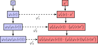
Figure 1: Computational graph for the computation of $f^{\prime}(c)\cdot x^{\prime}$.

$$\begin{array}[]{c}(c,\ x^{\prime})\\ (\varphi_{1}(c),\ \varphi^{\prime}_{1}(c)\cdot x^{\prime})\\ (\varphi_{2}\left(\varphi_{1}(c)\right),\ \varphi^{\prime}_{2}\left(\varphi_{1}(c)\right)\cdot\varphi^{\prime}_{1}(c)x^{\prime})\\ (\varphi_{3}\left(\varphi_{2}\left(\varphi_{1}(c)\right)\right),\ \varphi^{\prime}_{3}\left(\varphi_{2}\left(\varphi_{1}(c)\right)\right)\cdot\varphi^{\prime}_{2}\left(\varphi_{1}(c)\right)\varphi^{\prime}_{1}(c)x^{\prime})\end{array}$$

and taking the second entry of the final pair. As we see, the first element of each pair appears as an argument of the functions $\varphi_{i},\varphi^{\prime}_{i}$ in the following pair, while the second element appears as a factor (from the right) to the second element in the following pair.

Regarding the computation of $y^{\prime}\cdot f^{\prime}(c)$, we have obviously

$$y^{\prime}\cdot f^{\prime}(c)=y^{\prime}\cdot\varphi^{\prime}_{3}\left(\varphi_{2}\left(\varphi_{1}(c)\right)\right)\cdot\varphi^{\prime}_{2}\left(\varphi_{1}(c)\right)\cdot\varphi^{\prime}_{1}(c).$$

The computation of this derivative can now be achieved by the computing the following two lists of real numbers:

$$\begin{array}[]{c}c\\ \varphi_{1}(c)\\ \varphi_{2}(\varphi_{1}(c))\\ \varphi_{3}(\varphi_{2}(\varphi_{1}(c)))\end{array}\ \ \ \ \begin{array}[]{c}y^{\prime}\\ y^{\prime}\cdot\varphi^{\prime}_{3}\left(\varphi_{2}\left(\varphi_{1}(c)\right)\right)\\ y^{\prime}\varphi^{\prime}_{3}\left(\varphi_{2}\left(\varphi_{1}(c)\right)\right)\cdot\varphi^{\prime}_{2}\left(\varphi_{1}(c)\right)\\ y^{\prime}\varphi^{\prime}_{3}\left(\varphi_{2}\left(\varphi_{1}(c)\right)\right)\varphi^{\prime}_{2}\left(\varphi_{1}(c)\right)\cdot\varphi^{\prime}_{1}(c)\end{array}$$

and taking the last entry of the second list. Here, each entry (apart from $y^{\prime}$) in the second list consists of values of $\varphi^{\prime}_{i}$ evaluated at an element of the first list (note that the order is reversed) and the previous entry as a factor (from the left).

Figure 2: Computational graph for the computation of $y^{\prime}\cdot f^{\prime}(c)$.

In both examples, the computation of $\varphi_{3}(\varphi_{2}(\varphi_{1}(c)))$ is actually unnecessary to obtain the sought derivative. This value is, however, computed in all models we will consider in this article.

If now the functions $\varphi_{1},\varphi_{2},\varphi_{3}$ and their derivatives $\varphi^{\prime}_{1},\varphi^{\prime}_{2},\varphi^{\prime}_{3}$ are implemented in the system, then the evaluation of values $\varphi_{i}(v_{i}),\varphi^{\prime}_{i}(v_{i})$ for some $v_{i}$ means simply calling these functions/derivatives with suitable inputs. The computation of $f^{\prime}(c)\cdot x^{\prime}$ or $y^{\prime}\cdot f^{\prime}(c)$ then becomes nothing else than obtaining values $\varphi_{i}(v_{i}),\varphi^{\prime}_{i}(v_{i})$, performing a multiplication and passing the results on. That is, neither is some derivative evaluated symbolically, nor is some differential or difference quotient computed. In that sense, the derivative of $f$ is computed ‘automatically’.

2.2 The setting in general

As mentioned above, (First Order) Automatic Differentiation, in its simplest form, is concerned with the computation of derivatives of a differentiable function $f:X\to\mathbb{R}^{m}$, on an open set $X\subset\mathbb{R}^{n}$. The assumption made is that each $f_{j}:X\to\mathbb{R}$ in

$$f(x_{1},...,x_{n})=\left(\begin{array}[]{c}f_{1}(x_{1},...,x_{n})\\ \vdots\\ f_{m}(x_{1},...,x_{n})\end{array}\right),\ \ \textrm{for all}\ (x_{1},...,x_{n})\in X,$$

consists (to be defined more precisely later) of several sufficiently smooth so-called elementary (or elemental) functions $\varphi_{i}:U_{i}\to\mathbb{R}$, defined on open sets $U_{i}\subset\mathbb{R}^{n_{i}}$, with $i\in I$ for some index set $I$. The set of elementary functions $\{\varphi_{i}\ |\ i\in I\}$ has to be given and can, in principle, consist of arbitrary functions as long as these are sufficiently often differentiable. However, certain functions are essential for computational means, including addition and multiplication, constant, trigonometric, exponential functions etc. Figure 3 shows a table of such a (minimal) list. A more comprehensive list can be found, for example, in [9, Table 2.3].

Figure 3: Table of essential elementary functions according to Griewank and Walther [9]. The domains are chosen such that the functions are differentiable.

All elementary functions will be implemented in the system together with their gradients.

Automatic Differentiation now does not compute the actual mapping
$\mathbf{x}\mapsto J_{f}(\mathbf{x})$, which maps a vector $\mathbf{x}\in X$ to the Jacobian $J_{f}(\mathbf{x})$ of $f$ at $\mathbf{x}$. Instead, directional derivatives of $f$ or left-hand products of row-vectors with its Jacobian at a fixed vector $\mathbf{c}\in X$ are determined. That is, given $\mathbf{c}\in X$ and $\mathbf{\overset{\rightharpoonup}{x}}\in\mathbb{R}^{n}$ or $\mathbf{\overset{\leftharpoonup}{y}}\in\mathbb{R}^{1\times m}$, we determine either

$$J_{f}(\mathbf{c})\cdot\mathbf{\overset{\rightharpoonup}{x}}\ \ \ \ \ \textrm{or}\ \ \ \ \ \mathbf{\overset{\leftharpoonup}{y}}\cdot J_{f}(\mathbf{c}).$$

(This is not a subtle difference, since, while $\mathbf{x}\mapsto J_{f}(\mathbf{x})$ is a matrix-valued function, $J_{f}(\mathbf{c})\cdot\mathbf{\overset{\rightharpoonup}{x}}$ and $\mathbf{\overset{\leftharpoonup}{y}}\cdot J_{f}(\mathbf{c})$ are vectors or one-row matrices, respectively, in euclidean space.)

The computation of directional derivatives of $J_{f}(\mathbf{c})$ is referred to as the Forward Mode of AD, or Forward AD, while the computation of $\mathbf{\overset{\leftharpoonup}{y}}\cdot J_{f}(\mathbf{c})$ is referred to as the Reverse Mode of AD, or Reverse AD. We may give the following, informal descriptions:

Let $f:X\to\mathbb{R}^{m}$ consist of (not necessarily distinct!) elementary functions $\varphi_{1},...,\varphi_{\mu}$. Then

• Forward Automatic Differentiation is the computation of $J_{f}(\mathbf{c})\cdot\mathbf{\overset{\rightharpoonup}{x}}$ for fixed $\mathbf{c}\in X$ and $\mathbf{\overset{\rightharpoonup}{x}}\in\mathbb{R}^{n}$ through the successive computation of pairs of real numbers

  $$\left(\varphi_{1}(\mathbf{c_{1}}),\ \nabla\varphi_{1}(\mathbf{c_{1}})\cdot\mathbf{\overset{\rightharpoonup}{x_{1}}}\right),...,\left(\varphi_{\mu}(\mathbf{c_{\mu}}),\ \nabla\varphi_{\mu}(\mathbf{c_{\mu}})\cdot\mathbf{\overset{\rightharpoonup}{x_{\mu}}}\right)\in\mathbb{R}^{2}$$

  for suitable vectors $\mathbf{c_{i}}\in U_{i},\mathbf{\overset{\rightharpoonup}{x_{i}}}\in\mathbb{R}^{n_{i}}$, $i=1,...,\mu$.

• Reverse Automatic Differentiation is the computation of $\mathbf{\overset{\leftharpoonup}{y}}\cdot J_{f}(\mathbf{c})$ for fixed $\mathbf{c}\in X$ and $\mathbf{\overset{\leftharpoonup}{y}}\in\mathbb{R}^{1\times m}$ through the computation of the two lists of real numbers

  $$\varphi_{1}(\mathbf{c_{1}}),...,\varphi_{\mu}(\mathbf{c_{\mu}})\in\mathbb{R}$$

  and $$v_{1}\cdot\frac{\partial\varphi_{1}}{\partial v_{k}}(\mathbf{c_{1}})+v_{1,k}\ ,...,\ v_{\mu}\cdot\frac{\partial\varphi_{\mu}}{\partial v_{k}}(\mathbf{c_{\mu}})+v_{\mu,k}\ \in\mathbb{R},\ \ k=1,...,n_{i},$$

  for suitable vectors $\mathbf{c_{i}}\in U_{i}$ and suitable numbers $v_{i},v_{i,k}\in\mathbb{R}$, $i=1,...,\mu$.

Of course, the vectors and numbers $\mathbf{c_{i}},\mathbf{\overset{\rightharpoonup}{x_{i}}},v_{i},v_{i,k}$ are determined in a certain way; as is the order of in which the computations are performed.

As mentioned before, the function $f$ has to be constructed using elementary functions. Loosely speaking, we may say that $f$ has to be a composition of elements of $\{\varphi_{i}\ |\ i\in I\}$. However, this is not quite correct from a strictly mathematically point of view. Since all elementary functions are real-valued, it is clear that a composition $\varphi_{\mu}\circ\cdots\circ\varphi_{1}$ can not be defined, as soon as one of the $\varphi_{2},...,\varphi_{\mu}$ is multivariate. Admittedly, this is a rather technical and not really important issue, but, for completeness, we give the following inductive definition:

Definition 2.1.

• We call a function $h:X\to\mathbb{R}$ on open $X\subset\mathbb{R}^{n}$ automatically differentiable, if

  • $h\in\{\varphi_{i}\ |\ i\in I\}$ or

  • there exist functions $h_{k}:X_{k}\to\mathbb{R}$ on open sets $X_{k}\subset\mathbb{R}^{n_{k}}$, $k=1,...,\ell$, such that for all $\mathbf{x}=(x_{1},...,x_{n})\in X$, there exist $n_{0}\geq 0$ many $x_{0,1},...,x_{0,n_{0}}\in\{x_{1},...,x_{n}\}$ and, for $k=1,...,\ell-1$, $l=1,...,n_{k}$, there exist $n_{k}$ many $x_{k,l}\in\{x_{1},...,x_{n}\}\cap X_{k}$, with

    $$h(\mathbf{x})$$

    $$=h_{\ell}(x_{0,1},...,x_{0,n_{0}},h_{1}(x_{1,1},...,x_{1,n_{1}}),...,h_{\ell-1}(x_{\ell-1,1},...,x_{\ell-1,n_{\ell-1}})),$$

    and $h_{\ell}\in\{\varphi_{i}\ |\ i\in I\}$ and, for $k=1,...,\ell-1$, each $h_{k}$ is automatically differentiable.

• We call a function $f:X\to\mathbb{R}^{m}$ with $f(\mathbf{x})=\left(\begin{array}[]{c}f_{1}(\mathbf{x})\\ \vdots\\ f_{m}(\mathbf{x})\end{array}\right)$ for all $\mathbf{x}\in X$ automatically differentiable, if each $f_{j}:X\to\mathbb{R}$ is automatically differentiable.

Example 2.2.

The function $h:\mathbb{R}^{2}\to\mathbb{R}$ given by

$$h(x_{1},x_{2}) =\sin(x_{2})+5*\cos(x_{1}*x_{1}).$$

is automatically differentiable.

If we set $h_{3}=+$, $h_{1}=\sin$ and $h_{2}:\mathbb{R}\to\mathbb{R}$ with $h_{2}(x_{1})=5\cos(x_{1}^{2})$, we have

$$h(x_{1},x_{2})=h_{3}(h_{1}(x_{2}),h_{2}(x_{1})),$$

where clearly $h_{3}$ and $h_{1}$ are elementary. So consider $h_{2}$:

Set $h_{2,3}=*$, $h_{2,1}:\mathbb{R}\to\mathbb{R}$ with $h_{2,1}(x_{1})=5$ and $h_{2,2}:\mathbb{R}\to\mathbb{R}$ with $h_{2,2}(x_{1})=\cos(x_{1}^{2})$. Then

$$h_{2}(x_{1})=h_{2,3}(h_{2,1}(x_{1}),h_{2,2}(x_{1})),$$

where $h_{2,3}$ and $h_{2,1}$ are elementary. So consider $h_{2,2}$:

Setting $h_{2,2,2}=\cos$ and $h_{2,2,1}=*$ gives

$$h_{2,2}(x_{1})=h_{2,2,2}(h_{2,2,1}(x_{1},x_{1})),$$

where clearly, both, $h_{2,2,2}$ and $h_{2,2,1}$ are elementary functions.

Thus, by definition, $h_{2,2}$ is automatically differentiable, which makes $h_{2}$ automatically differentiable and, hence, $h$ is automatically differentiable.

From now on, without necessarily stating it explicitly, we will always assume that our function $f:X\to\mathbb{R}^{m}$ is automatically differentiable in the sense of Definition 2.1.

One may, rightfully, ask why we use an inductive description of automatically differentiable functions, instead of just describing them as compositions of suitable multi-variable, multi-dimensional mappings. However, from a computational point of view, one should note that an automatically differentiable $f:X\to\mathbb{R}^{m}$ will usually be given in the form of Definition 2.1, such that expressing $f$ as a composition may require additional work.

Nevertheless, expressing $f$ as a composition is indeed the basic step in an elementary description of Automatic Differentiation, which we describe in the next Section. We will describe other (equivalent) approaches which work directly with functions of the form of Definition 2.1 in later sections.

3 Forward AD—An elementary approach

In this approach, the function $f$ is described as a composition of multi-variate and multi-dimensional mappings. Differentiating this composition to obtain $J_{f}(\mathbf{c})\cdot\mathbf{\overset{\rightharpoonup}{x}}$, for given $\mathbf{c}\in X\subset\mathbb{R}^{n}$ and $\mathbf{\overset{\rightharpoonup}{x}}\in\mathbb{R}^{n}$, leads, by the chain rule, to a product of matrices. This method has, for example, been described in [21, Section 2] and, comprehensively, in the works of Griewank [8] and Griewank and Walther [9]. We follow mainly the notation of [8].

The simple idea is to express $f$ as a composition of the form

$$f=P_{Y}\circ\Phi_{\mu}\circ\cdots\circ\Phi_{1}\circ P_{X}.$$

Here, $P_{X}:X\to H$ is the (linear) natural embedding of the domain $X\subset\mathbb{R}^{n}$ into the so-called state space $H:=\mathbb{R}^{n+\mu}$, where $\mu$ is the total number of (not necessarily distinct) elementary functions $\varphi_{i}$ of which $f$ consists. Each
$\Phi_{i}:H\to H$, referred to as an elementary transition, corresponds to exactly one such elementary function. The mapping $P_{Y}:H\to\mathbb{R}^{m}$ is some suitable linear projection of $H$ down into $\mathbb{R}^{m}$.

Determining now $J_{f}(\mathbf{c})\cdot\mathbf{\overset{\rightharpoonup}{x}}$ for fixed $\mathbf{c}\in X$ and fixed $\mathbf{\overset{\rightharpoonup}{x}}\in\mathbb{R}^{n}$ becomes, by the chain rule, the evaluation of the matrix-vector product

$$J_{f}(\mathbf{c})\cdot\mathbf{\overset{\rightharpoonup}{x}} =P_{Y}\cdot\Phi^{\prime}_{\mu,\mathbf{c}}\ \cdots\ \Phi^{\prime}_{1,\mathbf{c}}\cdot P_{X}\cdot\mathbf{\overset{\rightharpoonup}{x}},$$ (3.1)

where $\Phi^{\prime}_{i,\mathbf{c}}$ denotes the Jacobian of $\Phi_{i}$ at $\left(\Phi_{i-1}\circ\cdots\circ\Phi_{1}\circ P_{X}\right)(\mathbf{c})$.

The process is now performed in a particular ordered fashion, which we describe in the following.

The evaluation of $f$ at some point $\mathbf{x}=(x_{1},...,x_{n})$ can be described by a so-called evaluation trace $\mathbf{v}^{[0]}=\mathbf{v}^{[0]}(\mathbf{x}),...,\mathbf{\mathbf{v}}^{[\mu]}=\mathbf{v}^{[\mu]}(\mathbf{x})$, where each $\mathbf{\mathbf{v}}^{[i]}\in H$ is a so-called state vector, representing the state of the evaluation after $i$ steps. More precisely, we set

$$\mathbf{\mathbf{v}}^{[0]}:=P_{X}(x_{1},...,x_{n})=(x_{1},...,x_{n},0,...,0)\ \ \textrm{and}\ \ \mathbf{\mathbf{v}}^{[i]}=\Phi_{i}(\mathbf{\mathbf{v}}^{[i-1]}),\ \ i=1,...,\mu.$$

The elementary transitions $\Phi_{i}$ are now given by imposing some suitable ordering on the $\mu$ elementary functions $\varphi_{k}$ of which $f$ consists, such that $\varphi_{i}$ is the $i$-th elementary function with respect to this order, and by setting

$$\Phi_{i}\left(\begin{array}[]{c}v_{1}\\ \vdots\\ v_{n+\mu}\end{array}\right)=\left(\begin{array}[]{c}v_{1}\\ \vdots\\ v_{n+i-1}\\ \varphi_{i}(v_{i_{1}},...,v_{i_{n_{i}}})\\ v_{n+i+1}\\ \vdots\\ v_{n+\mu}\end{array}\right),\ \ \textrm{for all}\ \left(\begin{array}[]{c}v_{1}\\ \vdots\\ v_{n+\mu}\end{array}\right)\in H,$$

and $v_{i_{1}},...,v_{i_{n_{i}}}\in\{v_{1},...,v_{n+i-1}\}\cap U_{i}$ (where $U_{i}\subset\mathbb{R}^{n_{i}}$ is the open domain of $\varphi_{i}$). Note that this is not a definition in the strict sense, since we neither specify the ordering of the $\varphi_{i}$, nor the arguments $v_{i_{1}},...,v_{i_{n_{i}}}$ of each $\varphi_{i}$. These will depend on the actual functions $f$ and $\varphi_{i}$. (Compare the example below.)

Therefore, we have

$$\mathbf{v}^{[i]}(\mathbf{x})=\Phi_{i}(\mathbf{\mathbf{v}}^{[i-1]}(\mathbf{x}))=\left(\begin{array}[]{c}\mathbf{\mathbf{v}}^{[i-1]}_{1}(\mathbf{x})=x_{1}\\ \vdots\\ \mathbf{\mathbf{v}}^{[i-1]}_{n}(\mathbf{x})=x_{n}\\ \vdots\\ \mathbf{\mathbf{v}}^{[i-1]}_{n+i-1}(\mathbf{x})\\ \varphi_{i}(v_{i_{1}}(\mathbf{x}),...,v_{i_{n_{i}}}(\mathbf{x}))\\ 0\\ \vdots\\ 0\end{array}\right)=\left(\begin{array}[]{c}\mathbf{\mathbf{v}}^{[i-1]}_{1}=x_{1}\\ \vdots\\ \mathbf{\mathbf{v}}^{[i-1]}_{n}=x_{n}\\ \vdots\\ \mathbf{\mathbf{v}}^{[i-1]}_{n+i-1}\\ \varphi_{i}(v_{i_{1}},...,v_{i_{n_{i}}})\\ 0\\ \vdots\\ 0\end{array}\right),$$

for $v_{i_{1}}=v_{i_{1}}(\mathbf{x}),...,v_{i_{n_{i}}}=v_{i_{n_{i}}}(\mathbf{x})\in\{\mathbf{\mathbf{v}}^{[i-1]}_{1},...,\mathbf{\mathbf{v}}^{[i-1]}_{n+i-1}\}\cap U_{i}$.

It is clear that, for the above to make sense, the ordering imposed on the elementary functions $\varphi_{k}$ must have the property that all arguments in $\varphi_{i}(v_{i_{1}},...,v_{i_{n_{i}}})$ have already been evaluated, before $\varphi_{i}$ is applied.

The definition of the projection $P_{Y}:H\to\mathbb{R}^{m}$ depends on the ordering imposed on the $\varphi_{k}$. If this ordering is such that we have

$$f_{1}(x_{1},...,x_{n})=\mathbf{\mathbf{v}}^{[\mu]}_{n+\mu-m}\ ,...,\ f_{m}(x_{1},...,x_{n})=\mathbf{\mathbf{v}}^{[\mu]}_{n+\mu},$$

we can obviously choose $P_{Y}(v_{1},...,v_{n+\mu})=(v_{n+\mu-m},...,v_{n+\mu})$.

Example 3.1.

The following is a trivial modification of an example taken from [8, page 332].

Consider the function $f:\mathbb{R}^{2}\to\mathbb{R}^{2}$ given by

$$f(x_{1},x_{2})=\left(\begin{array}[]{c}\exp(x_{1})*\sin(x_{1}+x_{2})\\ x_{2}\end{array}\right).$$

Choose $H=\mathbb{R}^{7}$ and $f=P_{Y}\circ\Phi_{5}\circ\Phi_{4}\circ\Phi_{3}\circ\Phi_{2}\circ\Phi_{1}\circ P_{X}$ with

$$P_{X}:\mathbb{R}^{2}\to\mathbb{R}^{7},\ \ \textrm{with}\ \ P_{X}(x_{1},x_{2})=(x_{1},x_{2},0,0,0,0,0),$$

$\Phi_{i}:\mathbb{R}^{7}\to\mathbb{R}^{7}$, $i=1,...,5$, with

$$\Phi_{1}\left(v_{1},v_{2},v_{3},v_{4},v_{5},v_{6},v_{7}\right)=(v_{1},v_{2},\exp(v_{1}),v_{4},v_{5},v_{6},v_{7}),$$

$$\Phi_{2}\left(v_{1},v_{2},v_{3},v_{4},v_{5},v_{6},v_{7}\right)=(v_{1},v_{2},v_{3},v_{1}+v_{2},v_{5},v_{6},v_{7}),$$

$$\Phi_{3}\left(v_{1},v_{2},v_{3},v_{4},v_{5},v_{6},v_{7}\right)=(v_{1},v_{2},v_{3},v_{4},\sin(v_{4}),v_{6},v_{7}),$$

$$\Phi_{4}\left(v_{1},v_{2},v_{3},v_{4},v_{5},v_{6},v_{7}\right)=(v_{1},v_{2},v_{3},v_{4},v_{5},v_{3}*v_{5},v_{7}),$$

$$\Phi_{5}\left(v_{1},v_{2},v_{3},v_{4},v_{5},v_{6},v_{7}\right)=\left(v_{1},v_{2},v_{3},v_{4},v_{5},v_{6},v_{2}\right)$$

and

$$P_{Y}:\mathbb{R}^{7}\to\mathbb{R}^{2},\ \ \textrm{with}\ \ P_{Y}(v_{1},v_{2},v_{3},v_{4},v_{5},v_{6},v_{7})=(v_{6},v_{7}).$$

Analogously to the evaluation of $f(\mathbf{x})$, the evaluation of the matrix-vector product (3.1) for some $\mathbf{c}\in\mathbb{R}^{n}$ and some $\mathbf{\overset{\rightharpoonup}{x}}=(x_{1}^{\prime},...,x_{n}^{\prime})\in\mathbb{R}^{n}$ can be expressed as an evaluation trace $\mathbf{v^{\prime}}^{[0]}=\mathbf{v^{\prime}}^{[0]}(\mathbf{c},\mathbf{\overset{\rightharpoonup}{x}}),...,\mathbf{v^{\prime}}^{[\mu]}=\mathbf{v^{\prime}}^{[\mu]}(\mathbf{c},\mathbf{\overset{\rightharpoonup}{x}})$, where

$$\mathbf{v^{\prime}}^{[0]}:=P_{X}\cdot\mathbf{\overset{\rightharpoonup}{x}}=(x_{1}^{\prime},...,x_{m}^{\prime},0,...,0)\ \ \ \textrm{and}\ \ \ \mathbf{\mathbf{v^{\prime}}}^{[i]}:=\Phi^{\prime}_{i,\mathbf{c}}\cdot\mathbf{v^{\prime}}^{[i-1]},\ \ i=1,...,\mu.$$

By the nature of the elementary transformations $\Phi_{i}$, each Jacobian
$\Phi^{\prime}_{i,\mathbf{c}}:=J_{\Phi_{i}}(\mathbf{v}^{[i-1]}(\mathbf{c}))$ will be of the form

$$\Phi^{\prime}_{i,\mathbf{c}}=\left(\begin{array}[]{cccccc}1&\cdots&0&0&\cdots&0\\ \vdots&\ddots&\vdots&\vdots&\cdots&\vdots\\ 0&\cdots&1&0&\cdots&0\\ \frac{\partial\varphi_{i}}{\partial v_{1}}(\cdots)&\cdots&\cdots&\cdots&\cdots&\frac{\partial\varphi_{i}}{\partial v_{n+\mu}}(\cdots)\\ 0&\cdots&0&1&\cdots&0\\ \vdots&\vdots&\vdots&\vdots&\ddots&\vdots\\ 0&\cdots&0&0&\cdots&1\end{array}\right)\leftarrow\ (n+i)\textrm{-th row},$$ (3.9)

where $\frac{\partial\varphi_{i}}{\partial v_{k}}(\cdots)=\frac{\partial\varphi_{i}}{\partial v_{k}}(v_{i_{1}}(\mathbf{c}),...,v_{i_{n_{i}}}(\mathbf{c}))$ is interpreted as $0$ if $\varphi_{i}$ does not depend on $v_{k}$.

Thus, each $\mathbf{\mathbf{v^{\prime}}}^{[i]}$ will be of the form

$$\mathbf{\mathbf{v^{\prime}}}^{[i]}=\left(\begin{array}[]{c}\mathbf{\mathbf{v^{\prime}}}^{[i-1]}_{1}=x^{\prime}_{1}\\ \vdots\\ \mathbf{\mathbf{v^{\prime}}}^{[i-1]}_{n}=x^{\prime}_{n}\\ \vdots\\ \mathbf{\mathbf{v^{\prime}}}^{[i-1]}_{n+i-1}\\ \nabla\varphi_{i}(v_{i_{1}},...,v_{i_{n_{i}}})\cdot\left(\begin{array}[]{c}v^{\prime}_{i_{1}}\\ \vdots\\ v^{\prime}_{i_{n_{i}}}\end{array}\right)\\ 0\\ \vdots\\ 0\end{array}\right),$$

for $v^{\prime}_{i_{1}}=v^{\prime}_{i_{1}}(\mathbf{c},\mathbf{\overset{\rightharpoonup}{x}}),...,v^{\prime}_{i_{n_{i}}}=v^{\prime}_{i_{n_{i}}}(\mathbf{c},\mathbf{\overset{\rightharpoonup}{x}})\in\{\mathbf{\mathbf{v^{\prime}}}^{[i-1]}_{1},...,\mathbf{v^{\prime}}^{[i-1]}_{n+i-1}\}$, where the
$v^{\prime}_{i_{1}},...,v^{\prime}_{i_{n_{i}}}$ correspond exactly to the $v_{i_{1}},...,v_{i_{n_{i}}}$. That is, if $v_{i_{j}}=\mathbf{v}^{[i-1]}_{l}(\mathbf{c})$, then $v^{\prime}_{i_{j}}=\mathbf{v^{\prime}}^{[i-1]}_{l}(\mathbf{c},\mathbf{\overset{\rightharpoonup}{x}})$.

The directional derivative of $f$ at $\mathbf{c}$ in direction of $\mathbf{\overset{\rightharpoonup}{x}}$ is then simply

$$J_{f}(\mathbf{c})\cdot\mathbf{\overset{\rightharpoonup}{x}}=P_{Y}\cdot\mathbf{v^{\prime}}^{[\mu]}.$$

Example 3.2.

Let $c_{1},c_{2},x^{\prime}_{1},x^{\prime}_{2}\in\mathbb{R}$. The computation of $J_{f}((c_{1},c_{2}))\cdot\left(\begin{array}[]{c}x^{\prime}_{1}\\ x^{\prime}_{2}\end{array}\right)$ with $f:\mathbb{R}^{2}\to\mathbb{R}^{2}$ given by

$$f(x_{1},x_{2})=\left(\begin{array}[]{c}\exp(x_{1})*\sin(x_{1}+x_{2})\\ x_{2}\end{array}\right)$$

has five evaluation trace pairs $[\mathbf{v}^{[0]},\mathbf{v^{\prime}}^{[0]}],...,[\mathbf{v}^{[5]},\mathbf{v^{\prime}}^{[5]}]$, where

$$\mathbf{v}^{[0]}=(c_{1},c_{2},0,0,0,0,0)\ \ \textrm{and}\ \ \mathbf{v^{\prime}}^{[0]}=(x^{\prime}_{1},x^{\prime}_{2},0,0,0,0,0)$$

and

$$\mathbf{\mathbf{v}}^{[5]}=\left(\begin{array}[]{c}c_{1}\\ c_{2}\\ \exp(c_{1})\\ c_{1}+c_{2}\\ \sin(c_{1}+c_{2})\\ \exp(c_{1})*\sin(c_{1}+c_{2})\\ c_{2}\end{array}\right),$$

$$\mathbf{\mathbf{v^{\prime}}}^{[5]}=\left(\begin{array}[]{c}x^{\prime}_{1}\\ x^{\prime}_{2}\\ \exp(c_{1})x^{\prime}_{1}\\ x^{\prime}_{1}+x^{\prime}_{2}\\ \cos(c_{1}+c_{2})(x^{\prime}_{1}+x^{\prime}_{2})\\ \sin(c_{1}+c_{2})\exp(c_{1})x^{\prime}_{1}+\exp(c_{1})\cos(c_{1}+c_{2})(x^{\prime}_{1}+x^{\prime}_{2})\\ x^{\prime}_{2}\end{array}\right).$$

Then $J_{f}((c_{1},c_{2}))\cdot\left(\begin{array}[]{c}x^{\prime}_{1}\\ x^{\prime}_{2}\end{array}\right)=P_{Y}\cdot\mathbf{\mathbf{v^{\prime}}}^{[5]}$, which is

$$\left(\begin{array}[]{c}\big{(}\sin(c_{1}+c_{2})\exp(c_{1})+\exp(c_{1})\cos(c_{1}+c_{2})\big{)}x^{\prime}_{1}+\exp(c_{1})\cos(c_{1}+c_{2})x^{\prime}_{2}\\ x^{\prime}_{2}\end{array}\right).$$

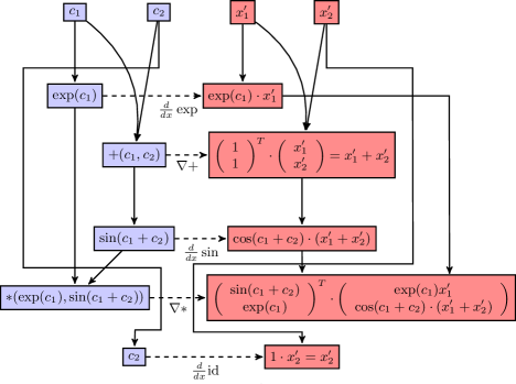
Figure 4: Computational graph for Example 3.2 with elements of $\mathbf{v}^{[5]}$ in blue and of $\mathbf{v^{\prime}}^{[5]}$ in red.

Note that in the evaluation process, given the $\Phi_{i}$, each pair $[\mathbf{v}^{[i]},\mathbf{v^{\prime}}^{[i]}]$ depends only on the previous pair $[\mathbf{v}^{[i-1]},\mathbf{v^{\prime}}^{[i-1]}]$ and the given vectors $\mathbf{c},\mathbf{\overset{\rightharpoonup}{x}}$. (Since $\mathbf{v}^{[i]}=\Phi_{i}(\mathbf{v}^{[i-1]})$ and $\mathbf{v^{\prime}}^{[i]}=J_{\Phi_{i}}(\mathbf{v}^{[i-1]}(\mathbf{c}))\cdot\mathbf{v^{\prime}}^{[i-1]}$.) Therefore, in an implementation, one can actually overwrite $[\mathbf{v}^{[i-1]},\mathbf{v^{\prime}}^{[i-1]}]$ by $[\mathbf{v}^{[i]},\mathbf{v^{\prime}}^{[i]}]$ in each step.

Note further that the $(n+i)$-th entry in each pair $[\mathbf{v}^{[i]},\mathbf{v^{\prime}}^{[i]}]$ is of the form

$$\left(\varphi_{i}(v_{i_{1}},...,v_{i_{n_{i}}}),\nabla\varphi_{i}(v_{i_{1}},...,v_{i_{n_{i}}})\cdot\left(\begin{array}[]{c}v^{\prime}_{i_{1}}\\ \vdots\\ v^{\prime}_{i_{n_{i}}}\end{array}\right)\right)\in\mathbb{R}^{2},$$ (3.13)

i.e. consisting of a value of $\varphi_{i}$ and a directional derivative of this elementary function. Since the previous $n+i-1$ entries are identical to the first
$n+i-1$ entries of $[\mathbf{v}^{[i-1]},\mathbf{v^{\prime}}^{[i-1]}]$, the computation of $[\mathbf{v}^{[i]},\mathbf{v^{\prime}}^{[i]}]$ is effectively the computation of (3.13).

We summarize the discussion of this Section:

Theorem 3.3.

By the above, given $\mathbf{c}\in X\subset\mathbb{R}^{n}$ and $\mathbf{\overset{\rightharpoonup}{x}}\in\mathbb{R}^{n}$, the evaluation of $J_{f}(\mathbf{c})\cdot\mathbf{\overset{\rightharpoonup}{x}}$ of an automatically differentiable function $f:X\to\mathbb{R}^{m}$ can be achieved by computing the evaluation trace pairs $[\mathbf{v}^{[i]},\mathbf{v^{\prime}}^{[i]}]$. This process is equivalent to the computation of the pairs (3.13).

The following section is concerned with a method which uses this last fact directly from the start. The approach about to be described also provides a better understanding on how an Automatic Differentiation system could actually be implemented. A question which may not be quite clear from the discussion so far.

4 Forward AD—An approach using Dual Numbers

Many descriptions and implementation of Forward AD actually use a slightly different approach than the elementary one that we have just described. Instead of expressing the function whose derivative one wants to compute as a composition, the main idea in this ‘alternative’ approach is to lift this function (and all elementary functions) to (a subset of) the algebra of dual numbers $\mathcal{D}$. This method has, for example, been described in [14], [20] and [23].

Dual numbers, introduced by Clifford [3], are defined as $\mathcal{D}:=(\mathbb{R}^{2},+,\cdot)$, where addition is defined component-wise, as usual, and multiplication is defined as

$$(x_{1},y_{1})\cdot(x_{2},y_{2}):=(x_{1}x_{2},x_{1}y_{2}+y_{1}x_{2}),\ \ \ \forall\ (x_{1},y_{1}),(x_{2},y_{2})\in\mathbb{R}^{2}.$$

It is easy to verify that $\mathcal{D}$ with these operations is an associative and commutative algebra over $\mathbb{R}$ with multiplicative unit $(1,0)$ and that the element $\varepsilon:=(0,1)$ is nilpotent of order two.

Analogously to a complex number, we write a dual number $z=(x,y)$ as $z=x+y\varepsilon$, where we identify each $x\in\mathbb{R}$ with $(x,0)$. We will further use the notation $(x,x^{\prime})$ instead of $(x,y)$, i.e. we write $z=x+x^{\prime}\varepsilon$. The $x^{\prime}$ in this representation will be referred to as the dual part of $z$.

We now define an extension of a differentiable, real-valued function
$h:X\to\mathbb{R}$, defined on open $X\subset\mathbb{R}^{n}$, to a function $\widehat{h}:\mathcal{D}^{n}\supset X\times\mathbb{R}^{n}\to\mathcal{D}$ defined on a subset of the dual numbers, by setting

$$\widehat{h}(x_{1}+x_{1}^{\prime}\varepsilon,...,x_{n}+x^{\prime}_{n}\varepsilon):=h(x_{1},...,x_{n})+\left(\nabla h(x_{1},...,x_{n})\cdot\left(\begin{array}[]{c}x^{\prime}_{1}\\ \vdots\\ x^{\prime}_{n}\end{array}\right)\right)\cdot\varepsilon.$$ (4.4)

This definition easily extends to differentiable functions $f:X\to\mathbb{R}^{m}$, where
$\widehat{f}:\mathcal{D}^{n}\supset X\times\mathbb{R}^{n}\to\mathcal{D}^{m}$ is defined via

$$\widehat{f}(x_{1}+x_{1}^{\prime}\varepsilon,...,x_{n}+x^{\prime}_{n}\varepsilon) :=\left(\begin{array}[]{c}\widehat{f}_{1}(x_{1}+x_{1}^{\prime}\varepsilon,...,x_{n}+x^{\prime}_{n}\varepsilon)\\ \vdots\\ \widehat{f}_{m}(x_{1}+x_{1}^{\prime}\varepsilon,...,x_{n}+x^{\prime}_{n}\varepsilon)\end{array}\right)$$ (4.8)

$$\ =f(x_{1},...,x_{n})+\left(J_{f}(x_{1},...,x_{n})\cdot\left(\begin{array}[]{c}x^{\prime}_{1}\\ \vdots\\ x^{\prime}_{n}\end{array}\right)\right)\varepsilon.$$ (4.12)

The following statement shows that definition (4.4) makes sense. I.e., that it is compatible with the natural extension of functions which are defined via usual arithmetic, i.e. polynomials, and analytic functions. That is:

Proposition 4.1.

Definition (4.4) is compatible with the “natural” extensions of

• real-valued constant functions

• projections of the form $(x_{1},..,x_{n})\mapsto x_{k}$,

• the arithmetic operations $+$, $*$ $:\mathbb{R}^{2}\to\mathbb{R}$ and
  $/:\{(x_{1},x_{2})\in\mathbb{R}^{2}\ |\ x_{2}\neq 0\}\to\mathbb{R}$, with

  $$+(x_{1},x_{2}):=x_{1}+x_{2},\ \ \ *(x_{1},x_{2}):=x_{1}\cdot x_{2},\ \ \ /(x_{1},x_{2}):=\frac{x_{1}}{x_{2}}\ .$$

• (multivariate) polynomials and rational functions

• (multivariate) real analytic functions

to subsets of $\mathcal{D}$, $\mathcal{D}^{2}$ or $\mathcal{D}^{n}$, respectively.

Proof.

(i) and (ii) follow easily from the definition.

(iii): We have

$$\widehat{+}\big{(}x_{1}+x^{\prime}_{1}\varepsilon,x_{2}+x^{\prime}_{2}\varepsilon\big{)}= +(x_{1},x_{2})+\left(\nabla+(x_{1},x_{2})\cdot\left(\begin{array}[]{c}x_{1}^{\prime}\\ x_{2}^{\prime}\end{array}\right)\right)\varepsilon$$

$$=(x_{1}+x_{2})+\left(\left(\begin{array}[]{c}1\\ 1\end{array}\right)^{T}\cdot\left(\begin{array}[]{c}x_{1}^{\prime}\\ x_{2}^{\prime}\end{array}\right)\right)\varepsilon$$

$$=(x_{1}+x_{2})+(x^{\prime}_{1}+x^{\prime}_{2})\varepsilon$$

$$=(x_{1}+x^{\prime}_{1}\varepsilon)+(x_{2}+x^{\prime}_{2}\varepsilon)$$

and, since $\varepsilon^{2}=0$,

$$\widehat{*}(x_{1}+x^{\prime}_{1}\varepsilon,x_{2}+x^{\prime}_{2}\varepsilon) =*(x_{1},x_{2})+\left(\nabla*(x_{1},x_{2})\cdot\left(\begin{array}[]{c}x_{1}^{\prime}\\ x_{2}^{\prime}\end{array}\right)\right)\varepsilon$$

$$=(x_{1}\cdot x_{2})+\left(\left(\begin{array}[]{c}x_{2}\\ x_{1}\end{array}\right)^{T}\cdot\left(\begin{array}[]{c}x_{1}^{\prime}\\ x_{2}^{\prime}\end{array}\right)\right)\varepsilon$$

$$=(x_{1}\cdot x_{2})+(x_{2}x^{\prime}_{1}+x_{1}x^{\prime}_{2})\varepsilon$$

$$=(x_{1}+x^{\prime}_{1}\varepsilon)\cdot(x_{2}+x^{\prime}_{2}\varepsilon).$$

Finally, considering division, it is easy to see that the multiplicative inverse of a dual numbers $x+x^{\prime}\varepsilon$ is defined if, and only if, $x\neq 0$ and given by $\frac{1}{x}+\left(-\frac{x^{\prime}}{x^{2}}\right)\varepsilon$.

Then, for $x_{2}\neq 0$, since $\varepsilon^{2}=0$,

$$\widehat{/}(x_{1}+x^{\prime}_{1}\varepsilon,x_{2}+x^{\prime}_{2}\varepsilon) =/(x_{1},x_{2})+\left(\nabla/(x_{1},x_{2})\cdot\left(\begin{array}[]{c}x_{1}^{\prime}\\ x_{2}^{\prime}\end{array}\right)\right)\varepsilon$$

$$=\frac{x_{1}}{x_{2}}+\left(\left(\begin{array}[]{c}\frac{1}{x_{2}}\\[4.30554pt] -\frac{x_{1}}{x_{2}^{2}}\end{array}\right)^{T}\cdot\left(\begin{array}[]{c}x_{1}^{\prime}\\ x_{2}^{\prime}\end{array}\right)\right)\varepsilon$$

$$=\frac{x_{1}}{x_{2}}+\left(\frac{x^{\prime}_{1}}{x_{2}}-\frac{x_{1}\cdot x^{\prime}_{2}}{x_{2}^{2}}\right)\varepsilon$$

$$=(x_{1}+x^{\prime}_{1}\varepsilon)\cdot\left(\frac{1}{x_{2}}+\left(-\frac{x^{\prime}_{2}}{x_{2}^{2}}\right)\varepsilon\right)$$

$$=\frac{x_{1}+x^{\prime}_{1}\varepsilon}{x_{2}+x^{\prime}_{2}\varepsilon}\ .$$

(iv): This will follow from Proposition 4.2 in connection with (iii).

(v): We will recall the definition of multi-variate Taylor series in Section 6. For the moment, let $T_{k}(h;\mathbf{c})$ denote the $k$-th degree (multi-variate) Taylor polynomial of $h:X\to\mathbb{R}$ about $\mathbf{c}\in X$. Since $h$ is real analytic, we have

$$T_{k}(h;\mathbf{c})(x_{1},...,x_{n})\to h(x_{1},...,x_{n})\ \ \ (k\to\infty)$$

for all $(x_{1},...,x_{n})\in V$, where $V$ is an open neighbourhood of $\mathbf{c}$. It is well-known, that then

$$\frac{\partial}{\partial x_{j}}T_{k}(h;\mathbf{c})(x_{1},...,x_{n})\to\frac{\partial}{\partial x_{j}}h(x_{1},...,x_{n})\ \ \ (k\to\infty)$$

on $V$ (see for example [13, Chapter II.1]). Since addition and multiplication are continuous, then also

$$\left(\nabla T_{k}(h;\mathbf{c})(x_{1},...,x_{n})\cdot\mathbf{\overset{\rightharpoonup}{x}}\right)\to\left(\nabla h(x_{1},...,x_{n})\cdot\mathbf{\overset{\rightharpoonup}{x}}\right)\ \ \ (k\to\infty)$$

on $V$, for any fixed $\mathbf{\overset{\rightharpoonup}{x}}=(x^{\prime}_{1},...,x^{\prime}_{n})\in\mathbb{R}^{n}$. Consequently,

$$\widehat{T_{k}}(h;\mathbf{c})(x_{1}+x^{\prime}_{1}\varepsilon,...,x_{n}+x^{\prime}_{n}\varepsilon)\to\widehat{h}(x_{1}+x^{\prime}_{1}\varepsilon,...,x_{n}+x^{\prime}_{n}\varepsilon)\ \ \ (k\to\infty),$$

for all $(x_{1}+x^{\prime}_{1}\varepsilon,...,x_{n}+x^{\prime}_{n}\varepsilon)\in V\times\mathbb{R}^{n}$. ∎

To use definition (4.4) for Automatic Differentiation, we need to show that it behaves well for automatically differentiable functions as defined in Definition 2.1. Basically, we need to show that (4.4) is compatible with the chain rule.

Proposition 4.2.

Let $h:X\to\mathbb{R}$ defined on open $X\subset\mathbb{R}^{n}$ be automatically differentiable, $h\notin\{\varphi_{i}\ |\ i\in I\}$. Then

$$\widehat{h}(\mathbf{x}+\mathbf{\overset{\rightharpoonup}{x}}\varepsilon)$$

$$=\widehat{h}_{\ell}(x_{0,1}+\varepsilon x^{\prime}_{0,1},...,x_{0,n_{0}}+\varepsilon x^{\prime}_{0,n},\widehat{h}_{1}(x_{1,1}+\varepsilon x^{\prime}_{1,1},...,x_{1,n_{1}}+\varepsilon x^{\prime}_{1,n_{1}}),$$

$$\ \ \ \ \ ...,\widehat{h}_{\ell-1}(x_{\ell-1,1}+\varepsilon x^{\prime}_{\ell-1,1},...,x_{\ell-1,n_{\ell-1}}+\varepsilon x^{\prime}_{\ell-1,n_{\ell-1}})),$$ (4.13)

for all $\mathbf{x}+\varepsilon\mathbf{\overset{\rightharpoonup}{x}}:=(x_{1}+\varepsilon x^{\prime}_{1},...,x_{n}+\varepsilon x^{\prime}_{n})\in X\times\mathbb{R}^{n}$, with
$x_{k,i}+x^{\prime}_{k,i}\in\{x_{1}+\varepsilon x^{\prime}_{1},...,x_{n}+\varepsilon x^{\prime}_{n}\}\cap X_{k}$.

Proof.

We prove this statement by direct computation. In the following, denote

$$\mathbf{x_{k}}:=(x_{k,1},...,x_{k,n_{k}})\in X_{k}\subset\mathbb{R}^{n_{k}}\ \ \textrm{and}\ \ \mathbf{\overset{\rightharpoonup}{x}_{k}}:=(x^{\prime}_{k,1},...x^{\prime}_{k,n_{k}})\in X_{k}\times\mathbb{R}^{n_{k}}.$$

Then the right hand-side of equation (4.2) is equal to

$$\widehat{h_{\ell}}\left(\mathbf{x_{0}},h_{1}(\mathbf{x_{1}})+\left(\nabla h_{1}(\mathbf{x_{1}})\cdot\mathbf{\overset{\rightharpoonup}{x}_{k}}\right)\varepsilon,\right.$$

$$\left.\ \ \ \ \ ...,h_{\ell-1}(\mathbf{x_{\ell-1}})+\left(\nabla h_{\ell-1}(\mathbf{x_{\ell-1}})\cdot\mathbf{\overset{\rightharpoonup}{x}_{\ell-1}}\right)\varepsilon\right)$$ (4.14)

$$=h_{\ell}\left(\mathbf{x_{0}},h_{1}(\mathbf{x_{1}}),...,h_{\ell-1}(\mathbf{x_{\ell-1}})\right)+\left(\nabla h_{\ell}\left(...\right)\cdot\left(\begin{array}[]{c}x^{\prime}_{0,1}\\ \vdots\\ x^{\prime}_{0,n}\\ \nabla h_{1}(\mathbf{x_{1}})\cdot\mathbf{\overset{\rightharpoonup}{x}_{1}}\\ \vdots\\ \nabla h_{\ell-1}(\mathbf{x_{\ell-1}})\cdot\mathbf{\overset{\rightharpoonup}{x}_{\ell-1}}\end{array}\right)\right)\varepsilon,$$ (4.21)

where

$$\nabla h_{\ell}\left(...\right) :=\nabla h_{\ell}\left(\mathbf{x_{0}},h_{1}(\mathbf{x_{1}}),...,h_{\ell-1}(\mathbf{x_{\ell-1}})\right)$$

$$=\frac{dh_{\ell}}{d(\mathbf{x_{0}},h_{1}(\mathbf{x_{1}}),...,h_{\ell-1}(\mathbf{x_{\ell-1}}))}(\mathbf{x_{0}},h_{1}(\mathbf{x_{1}}),...,h_{\ell-1}(\mathbf{x_{\ell-1}})).$$

The left hand side of (4.2) is obviously equal to

$$h(\mathbf{x})+\left(\nabla h(\mathbf{x})\cdot\mathbf{\overset{\rightharpoonup}{x}}\right)\cdot\varepsilon.$$ (4.22)

By assumption, $h(\mathbf{x})=h_{\ell}(\mathbf{x_{0}},h_{1}(\mathbf{x_{1}}),...,h_{\ell-1}(\mathbf{x_{\ell-1}}))$. Further, by the chain rule,

$$\nabla h(\mathbf{x})\cdot\mathbf{\overset{\rightharpoonup}{x}} =\frac{dh_{\ell}}{d\mathbf{x}}(\mathbf{x_{0}},h_{1}(\mathbf{x_{1}}),...,h_{\ell-1}(\mathbf{x_{\ell-1}}))\cdot\mathbf{\overset{\rightharpoonup}{x}}$$

$$=\nabla h_{\ell}\left(\mathbf{x_{0}},h_{1}(\mathbf{x_{1}}),...,h_{\ell-1}(\mathbf{x_{\ell-1}})\right)$$

$$\ \ \ \ \cdot\frac{d\left(\mathbf{x}\mapsto(\mathbf{x_{0}},h_{1}(\mathbf{x_{1}}),...,h_{\ell-1}(\mathbf{x_{\ell-1}})\right)}{d\mathbf{x}}\left(\mathbf{x}\right)\cdot\mathbf{\overset{\rightharpoonup}{x}}.$$

Now, $\frac{d\left(\mathbf{x}\mapsto(\mathbf{x_{0}},h_{1}(\mathbf{x_{1}}),...,h_{\ell-1}(\mathbf{x_{\ell-1}})\right)}{d\mathbf{x}}\left(\mathbf{x}\right)$ equals

$$\left(\begin{array}[]{ccc}\frac{\partial(\mathbf{x}\mapsto x_{0,1})}{\partial x_{1}}(\mathbf{x})&\cdots&\frac{\partial(\mathbf{x}\mapsto x_{0,1})}{\partial x_{n}}(\mathbf{x})\\ \vdots&\vdots&\vdots\\ \frac{\partial(\mathbf{x}\mapsto x_{0,n_{0}})}{\partial x_{1}}(\mathbf{x})&\cdots&\frac{\partial(\mathbf{x}\mapsto x_{0,n_{0}})}{\partial x_{n}}(\mathbf{x})\\[4.30554pt] \frac{\partial(\mathbf{x}\mapsto h_{1}(\mathbf{x_{1}}))}{\partial x_{1}}(\mathbf{x})&\cdots&\frac{\partial(\mathbf{x}\mapsto h_{1}(\mathbf{x_{1}}))}{\partial x_{n}}(\mathbf{x})\\[4.30554pt] \vdots&\vdots&\vdots\\ \frac{\partial(\mathbf{x}\mapsto h_{\ell-1}(\mathbf{x_{\ell-1}}))}{\partial x_{1}}(\mathbf{x})&\cdots&\frac{\partial(\mathbf{x}\mapsto h_{\ell-1}(\mathbf{x_{\ell-1}}))}{\partial x_{n}}(\mathbf{x})\end{array}\right)$$

Hence,

$$\frac{d\left(\mathbf{x}\mapsto(\mathbf{x_{0}},h_{1}(\mathbf{x_{1}}),...,h_{\ell-1}(\mathbf{x_{\ell-1}})\right)}{d\mathbf{x}}\left(\mathbf{x}\right)\cdot\mathbf{\overset{\rightharpoonup}{x}}=\left(\begin{array}[]{c}x^{\prime}_{0,1}\\ \vdots\\ x^{\prime}_{0,n}\\ \nabla h_{1}(\mathbf{\overset{\rightharpoonup}{x}_{1}})\cdot\mathbf{\overset{\rightharpoonup}{x}_{1}}\\ \vdots\\ \nabla h_{\ell-1}(\mathbf{x_{\ell-1}})\cdot\mathbf{\overset{\rightharpoonup}{x}_{\ell-1}}\end{array}\right)$$

Thus, (4) equals (4.22) and we are done. ∎

We can now automatically compute directional derivatives $J_{f}(\mathbf{c})\cdot\mathbf{\overset{\rightharpoonup}{x}}$ of an automatically differentiable function $f:X\to\mathbb{R}^{m}$, on open $X\subset\mathbb{R}^{n}$, at fixed $\mathbf{c}=(c_{1},...,c_{n})\in\mathbb{R}^{n}$ in direction of fixed $\mathbf{\overset{\rightharpoonup}{x}}=(x_{1}^{\prime},...,x_{n}^{\prime})\in\mathbb{R}^{n}$ by computing the directional derivatives $\nabla f_{j}(\mathbf{c})\cdot\mathbf{\overset{\rightharpoonup}{x}}$ in the following way:

Theorem 4.3.

Assume that definition 4.4 is implemented for all elementary functions in the set $\{\varphi_{i}\ |\ i\in I\}$. Then the directional derivative $\nabla f_{j}(\mathbf{c})\cdot\mathbf{\overset{\rightharpoonup}{x}}$ of an automatically differentiable function $f_{j}:X\to\mathbb{R}$ can be computed ‘automatically’ through extending $f_{j}$ to $X\times\mathbb{R}^{n}\subset\mathcal{D}^{n}$, and evaluating the dual part of $\widehat{f}_{j}(c_{1}+x^{\prime}_{1}\varepsilon,...,c_{n}+x^{\prime}_{n}\varepsilon)$.

Proof.

Each $f_{j}$ is automatically differentiable. By assumption, the case $f_{j}\in\{\varphi_{i}\ |\ i\in I\}$ is clear: We simply obtain the pair $\widehat{f}_{j}(c_{1}+x^{\prime}_{1}\varepsilon,...,c_{n}+x^{\prime}_{n}\varepsilon)$ by calling $f_{j}$ and $\nabla f_{j}$ and computing the gradient-vector product. The sought directional derivative is the dual part (second entry) of that pair.

So assume that there exists real-valued $h_{1},...,h_{\ell}$ on open sets $X_{k}\subset\mathbb{R}^{n_{k}}$, such that for all $\mathbf{x}\in X$,

$$f_{j}(\mathbf{x})=h_{\ell}(x_{0,1},...,x_{0,n_{0}},h_{1}(x_{1,1},...,x_{1,n_{1}}),...,h_{\ell-1}(x_{\ell-1,1},...,x_{\ell-1,n_{\ell-1}})),$$

for suitable $x_{k,j}$, with $h_{\ell}\in\{\varphi_{i}\ |\ i\in I\}$ and $h_{1},...,h_{\ell-1}$ automatically differentiable.

We proceed by induction on the depth of $f_{j}$.

Base case: Assume that each $h_{1},...,h_{\ell}\in\{\varphi_{i}\ |\ i\in I\}$. Extending $f_{j}$ to $X\times\mathbb{R}^{n}\subset\mathcal{D}^{n}$ leads to the extension of $h_{1},...,h_{\ell}$ to sets $X_{k}\times\mathbb{R}^{n_{k}}\subset\mathcal{D}^{n_{k}}$. Since definition 4.4 is implemented for all functions in $\{\varphi_{i}\ |\ i\in I\}$,

$$\widehat{h}_{k}(c_{k,1}+x^{\prime}_{k,1}\varepsilon,...,c_{k,n_{k}}+x^{\prime}_{k,n_{k}}\varepsilon)$$

is defined for all $h_{k}$ and computed by calling $h_{k}$ and all $\nabla h_{k}$ with suitable inputs and computing the gradient-vector product. By Proposition 4.2, the computation of

$$\widehat{h}_{\ell}(c_{0,1}+x^{\prime}_{0,1}\varepsilon,...,c_{0,n_{0}}+x^{\prime}_{0,n_{0}}\varepsilon,\widehat{h}_{1}(\cdots),...,\widehat{h}_{\ell-1}(\cdots)),$$

which is performed last, gives $\widehat{f}_{j}(c_{1}+x^{\prime}_{1}\varepsilon,...,c_{n}+x^{\prime}_{n}\varepsilon)$, whose dual part is $\nabla f_{j}(\mathbf{c})\cdot\mathbf{\overset{\rightharpoonup}{x}}$.

Induction step: Assume that $h_{j_{0}}\in\{h_{1},...,h_{\ell-1}\}$ is not an elementary function. Again, we extend $f_{j}$ to $X\times\mathbb{R}^{n}\subset\mathcal{D}^{n}$, which leads to the extension of $h_{1},...,h_{\ell}$ to sets $X_{k}\times\mathbb{R}^{n_{k}}\subset\mathcal{D}^{n_{k}}$. Since $h_{j_{0}}$ is still automatically differentiable

$$\widehat{h}_{j_{0}}(c_{j_{0},1}+x^{\prime}_{j_{0},1}\varepsilon,...,c_{j_{0},n_{j_{0}}}+x^{\prime}_{j_{0},n_{j_{0}}}\varepsilon)$$

is computed by Induction Assumption. Then again, the computation of

$$\widehat{h}_{\ell}(c_{0,1}+x^{\prime}_{0,1}\varepsilon,...,c_{0,n_{0}}+x^{\prime}_{0,n_{0}}\varepsilon,\widehat{h}_{1}(\cdots),...,\widehat{h}_{\ell-1}(\cdots))$$

(note that $h_{\ell}$ is elementary) gives, by Proposition 4.2, the dual number $\widehat{f}_{j}(c_{1}+x^{\prime}_{1}\varepsilon,...,c_{n}+x^{\prime}_{n}\varepsilon)$. ∎

Example 4.4.

Consider the function $f:\mathbb{R}^{2}\to\mathbb{R}$ given by

$$f(x_{1},x_{2}) =x_{2}*\cos(x_{1}^{2}+3)=x_{2}*\cos(x_{1}*x_{1}+3).$$

Let $c_{1},c_{2},x^{\prime}_{1},x^{\prime}_{2}\in\mathbb{R}$. We evaluate the value of $\widehat{f}$ at $c_{1}+x^{\prime}_{1}\varepsilon$ and $c_{2}+x^{\prime}_{2}\varepsilon$. By definition (4.4), Proposition 4.1 and Proposition 4.2,

$$\widehat{f}(c_{1}+x^{\prime}_{1}\varepsilon,c_{2}+x^{\prime}_{2}\varepsilon)$$

$$=(c_{2}+x^{\prime}_{2}\varepsilon)*\cos((c_{1}+x^{\prime}_{1}\varepsilon)^{2}+3)$$

$$=(c_{2}+x^{\prime}_{2}\varepsilon)*\cos(c_{1}^{2}+2c_{1}x^{\prime}_{1}\varepsilon+3)$$

$$=(c_{2}+x^{\prime}_{2}\varepsilon)*\cos((c_{1}^{2}+3)+2c_{1}x^{\prime}_{1}\varepsilon)$$

$$=(c_{2}+x^{\prime}_{2}\varepsilon)*(\cos(c_{1}^{2}+3)-\sin(c_{1}^{2}+3)2c_{1}x^{\prime}_{1}\varepsilon)$$

$$=c_{2}\cos(c_{1}^{2}+3)+\left(-2c_{1}c_{2}\sin(c_{1}^{2}+3)x^{\prime}_{1}+\cos(c_{1}^{2}+3)x^{\prime}_{2}\right)\varepsilon.$$

By Theorem 4.3, the dual part of this expression is $\nabla f(c_{1},c_{2})\cdot\left(\begin{array}[]{c}x^{\prime}_{1}\\ x^{\prime}_{2}\end{array}\right)$. That is,

$$\nabla f(c_{1},c_{2})\cdot\left(\begin{array}[]{c}x^{\prime}_{1}\\ x^{\prime}_{2}\end{array}\right)=-2c_{1}c_{2}\sin(c_{1}^{2}+3)x^{\prime}_{1}+\cos(c_{1}^{2}+3))x^{\prime}_{2}.$$

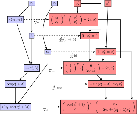
Figure 5: Computational graph for Example 4.4 with primal parts in blue and dual parts in red.

Figure 6: Minimal Haskell example, showing the implementation of Forward AD for Example 4.4 and the test case $\frac{\partial f}{\partial x_{1}}(5,2)$. Compare also the basically identical work in [17, Subsection 2.1].

Thus, a (basic) implementation of an Automatic Differentiation System can be realised by implementing (4.4) for all elementary functions. Usually, this is done by simply overloading elementary functions. Constant functions will usually be identified with real numbers, which themselves will be lifted to dual number with zero dual part (see Figure 6).

Note again that at no time during the described process any symbolic differentiation takes place. Instead, since each ‘top-level’ function $h_{\ell}$ of an automatically differentiable function is elementary, we are computing and passing on pairs

$$\left(\varphi_{i}(c_{i,1},...,c_{i,n_{i}}),\nabla\varphi_{i}(c_{i,1},...,c_{i,n_{i}})\cdot\left(\begin{array}[]{c}x^{\prime}_{i,1}\\ \vdots\\ x^{\prime}_{i,n_{i}}\end{array}\right)\right)\in\mathbb{R}^{2},$$ (4.26)

which computes ‘automatically’ the directional derivatives $\nabla f_{j}(\mathbf{c})\cdot\mathbf{\overset{\rightharpoonup}{x}}$ and, therefore, the directional derivative $J_{f}(\mathbf{c})\cdot\mathbf{\overset{\rightharpoonup}{x}}$.

Note further that the pairs (4.26) are exactly the same pairs as the ones in (3.13). This means that the processes described in this and in the previous Section reduce to exactly the same computations.

Indeed, if we store the pairs $(c_{i},x^{\prime}_{i})$ and (4.26) in an array, we obtain the evaluation trace pairs $[\mathbf{v}^{[i]},\mathbf{v^{\prime}}^{[i]}]$. In summary:

Theorem 4.5.

By the above, given $\mathbf{c}\in X\subset\mathbb{R}^{n}$ and $\mathbf{\overset{\rightharpoonup}{x}}\in\mathbb{R}^{n}$, the evaluation of $J_{f}(\mathbf{c})\cdot\mathbf{\overset{\rightharpoonup}{x}}$ of an automatically differentiable function $f:X\to\mathbb{R}^{m}$ can be achieved through the lifting of each $f_{j}$ to a function $\widehat{f}_{j}:X\times\mathbb{R}^{n}\to\mathcal{D}$ as defined in (4.4) and by evaluating $\widehat{f}_{j}(c_{1}+x^{\prime}_{1}\varepsilon,...,c_{n}+x^{\prime}_{n}\varepsilon)$. This process is equivalent to the computation of the evaluation trace pairs $[\mathbf{v}^{[i]},\mathbf{v^{\prime}}^{[i]}]$, as described in the previous section, and to the computation of the pairs (4.26) in suitable order.

5 Comparison with Symbolic Differentiation—Some Thoughts on Complexity

Before we move on to further descriptions of Forward AD and to a brief description of the Reverse Mode, we take a look at some example cases to demonstrate how Automatic Differentiation solves some complexity issues which appear in systems which use symbolic differentiation.

Assume that we want to obtain the derivative of a composition $f$ of uni-variate elementary functions $\varphi_{1},...,\varphi_{n}:\mathbb{R}\to\mathbb{R}$, that is,

$$f=\varphi_{n}\circ\cdots\circ\varphi_{1},$$

at a certain value $c\in\mathbb{R}$.

A symbolic differentiation system will first use the chain rule to determine the derivative function $f^{\prime}$, which is given by

$$f^{\prime}(x)=\varphi^{\prime}_{n}(\varphi_{n-1}(\cdots(\varphi_{1}(x))))\cdot\varphi^{\prime}_{n-1}(\varphi_{n-2}(\cdots(\varphi_{1}(x))))\cdot\ \cdots\ \cdot\varphi^{\prime}_{2}(\varphi_{1}(x))\cdot\varphi^{\prime}_{1}(x),$$

for all $x\in\mathbb{R}$, and then compute $f^{\prime}(c)$ by substituting $x$ by $c$. That is, each factor is computed and the results are multiplied. Hence, the system computes the following values:

$$\varphi^{\prime}_{1}(c)$$

$$\varphi_{1}(c),\ \varphi^{\prime}_{2}(\varphi_{1}(c))$$

$$\varphi_{1}(c),\ \varphi_{2}(\varphi_{1}(c)),\ \varphi^{\prime}_{3}(\varphi_{2}(\varphi_{1}(c)))$$

$$\varphi_{1}(c),\ \varphi_{2}(\varphi_{1}(c)),\ \varphi_{3}(\varphi_{2}(\varphi_{1}(c))),\ \varphi^{\prime}_{4}(\varphi_{3}(\varphi_{2}(\varphi_{1}(c))))$$

$$\vdots$$

$$\varphi_{1}(c),\ \varphi_{2}(\varphi_{1}(c)),\ \varphi_{3}(\varphi_{2}(\varphi_{1}(c))),...,\ \varphi^{\prime}_{n}(\varphi_{n-1}(\cdots(\varphi_{1}(c))))$$

As we see many expressions will be computed multiple times (loss of sharing). If we ignore the time the system needs to determine $f^{\prime}$, as well as the time for performing multiplications, and set the cost for the computation of each value of $\varphi_{i},\varphi^{\prime}_{i}$ as $1$, then the total cost of computing $f^{\prime}(c)$ is

$$1+2+3+\cdots+n=\sum_{k=1}^{n}k=\frac{n(n+1)}{2}\in\mathcal{O}(n^{2}).$$

In comparison, a Forward Automatic Differentiation system will perform a computation of pairs starting with $\big{(}\varphi_{1}(c),\varphi^{\prime}_{1}(c)\cdot 1\big{)}$, where the $(i+1)$-st pair for $i\geq 1$ looks like

$$\big{(}\varphi_{i+1}(v_{i}),\ \varphi^{\prime}_{i+1}(v_{i})\cdot v^{\prime}_{i}\big{)},$$

for some $v_{i},v^{\prime}_{i}\in\mathbb{R}$. See the computational graph in Figure 1 in Subsection 2.1 for the case $n=3$ (set $x^{\prime}=1$). If we again ignore costs for multiplications, the cost for evaluating each pair is $2$. Hence, the total costs of evaluating $f^{\prime}(c)$ via Automatic Differentiation is $2n$.

In [19] the example of a product of the form

$$f=\varphi_{n}*\cdots*\varphi_{1}=*(\varphi_{n},\ *(\varphi_{n-1},*(\cdots(*(\varphi_{2},\varphi_{1})))))$$

is given. Here, the evaluation of the derivative of $f^{\prime}(c)$ at some $c\in\mathbb{R}$ by a symbolic differentiation system will first use the product rule to compute $f^{\prime}$ given by

$$f^{\prime}(x)= \varphi^{\prime}_{n}(x)\cdot(\varphi_{n-1}(x)\cdots\varphi_{1}(x))+\varphi^{\prime}_{n-1}(x)\cdot(\varphi_{n}(x)\cdot\varphi_{n-2}(x)\cdots\varphi_{1}(x))$$

$$+\cdots+\varphi^{\prime}_{1}(x)\cdot(\varphi_{n}(x)\cdots\varphi_{2}(x)),$$

for all $x\in\mathbb{R}$, and then again substitute $x$ by $c$. Again, many function values will be computed multiple times. Since we have $n$ functions in each summand and $n$ summands, ignoring cost for multiplications and addition, the computation of $f^{\prime}(c)$ has a total cost of $n^{2}$.

In contrast, a Forward Automatic Differentiation system will compute pairs starting with

$$\big{(}\varphi_{1}(c),\ \varphi^{\prime}_{1}(c)\cdot 1\big{)},\ \big{(}\varphi_{2}(c),\ \varphi^{\prime}_{2}(c)\cdot 1\big{)},\ \left(\varphi_{1}(c)*\varphi_{2}(c),\ \left(\begin{array}[]{c}\varphi_{2}(c)\\ \varphi_{1}(c)\end{array}\right)^{T}\cdot\left(\begin{array}[]{c}\varphi_{1}^{\prime}(c)\\ \varphi^{\prime}_{2}(c)\end{array}\right)\right)$$

where the remaining pairs for $i\geq 2$ look like

$$\big{(}\varphi_{i+1}(c),\ \varphi^{\prime}_{i+1}(c)\cdot 1\big{)},\ \ \left(\varphi_{i+1}(c)*v_{i},\ \left(\begin{array}[]{c}v_{i}\\ \varphi_{i+1}(c)\end{array}\right)^{T}\cdot\left(\begin{array}[]{c}\varphi^{\prime}_{i+1}(c)\\ v^{\prime}_{i}\end{array}\right)\right)$$

for some $v_{i},v^{\prime}_{i}\in\mathbb{R}$. Since the $3$rd, $5$th, $7$th etc. pairs are those which are created by lifting $*$ to the dual numbers, they contain only additions and multiplications of values which have already been computed. Hence, for simplicity, we may discard these pairs with regards to the costs of the evaluations of $f^{\prime}(c)$. Thus, the total cost of computing $f^{\prime}(c)$ is the cost of computing the $n$ pairs $\big{(}\varphi_{i+1}(c),\ \varphi^{\prime}_{i+1}(c)\cdot 1\big{)}$ which is $2n$.

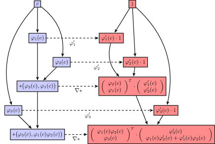
Figure 7: Computational graph for the computation of $f^{\prime}(c)=\frac{d}{dx}\left(\varphi_{n}*\cdots*\varphi_{1}\right)(c)$ in the case $n=3$.

A further advantage of Forward AD, at least in many implementation, is the efficient handling of common intermediate expressions feeding into several subsequent intermediates. Consider for this the case of a sum of the $n$ elementary uni-variate functions $\varphi_{i}$ each composed with another univariate elementary function $\psi:\mathbb{R}\to\mathbb{R}$:

$$f=(\varphi_{1}\circ\psi)+\cdots+(\varphi_{n}\circ\psi)=+(\varphi_{n}\circ\psi,\ +(\varphi_{n-1}\circ\psi,+(\cdots(+(\varphi_{2}\circ\psi,\varphi_{1}\circ\psi)))))$$

The derivative $f^{\prime}$ is in this case obviously given by

$$f^{\prime}(x)=\psi^{\prime}(x)\cdot\varphi^{\prime}_{1}(\psi(x))+\cdots+\psi^{\prime}(x)\cdot\varphi^{\prime}_{n}(\psi(x)),$$

for all $x\in\mathbb{R}$. To determine $f^{\prime}(c)$, a symbolic differentiation system will evaluate $\psi(c)$ in each summand, that is $n$ times (and possibly, if the expression $\psi^{\prime}(x)$ is not factored out, $\psi^{\prime}(c)$ as well $n$-times). Hence, the computational cost of evaluating $f^{\prime}(c)$ is at least $2n+1$ (if $\psi^{\prime}(x)$ is factored out, $3n$ otherwise), where we again ignore costs for additions and multiplications and for determining the derivative function $f^{\prime}$. If we want to obtain the value $f(c)$, too, the cost increases to $4n+1$ (or $6n$, respectively).

In this particular case, some realisations of a Forward Automatic Differentiation system might evaluate $\psi^{\prime}(c)$ $n$-times as well. However, in many implementations the value $\psi(c)$ will be assigned to a new variable $z$, such that

$$f(c)=\varphi_{1}(z)+\cdots+\varphi_{n}(z)\ \ \textrm{and}\ \ f^{\prime}(c)=z^{\prime}\cdot\varphi^{\prime}_{1}(z)+\cdots+z^{\prime}\cdot\varphi^{\prime}_{n}(z),$$

where $z^{\prime}:=\psi^{\prime}(c)$. The Forward AD system will then compute pairs starting with

$$\big{(}z,\ z^{\prime}\cdot 1\big{)},\ \ \big{(}\varphi_{1}(z),\ \varphi^{\prime}_{1}(z)\cdot z^{\prime}\big{)},\ \ \big{(}\varphi_{2}(z),\ \varphi^{\prime}_{2}(z)\cdot z^{\prime}\big{)},$$

$$\big{(}\varphi_{1}(z)+\varphi_{2}(z),\ \varphi^{\prime}_{1}(z)\cdot z^{\prime}+\varphi^{\prime}_{2}(z)\cdot z^{\prime}\big{)}\ \ \textrm{etc.}$$

Clearly, in this process the values (numbers) $\psi(c)=z$ and $\psi^{\prime}(c)=z^{\prime}$ are computed only once. If we again ignore costs for additions and multiplications (including the cost for computing pairs created by lifting $+$), the total cost of determining both $f(c)$ and $f^{\prime}(c)$ is the cost of computing the $n+1$ pairs $\big{(}z,\ z^{\prime}\cdot 1\big{)}$, $\big{(}\varphi_{i}(z),\ \varphi^{\prime}_{i}(z)\cdot z^{\prime}\big{)}$, $i=1,...,n$, which is $2n+2$.

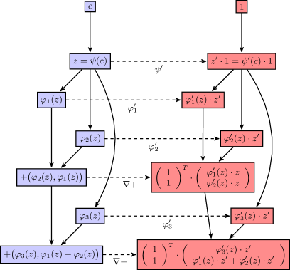
Figure 8: Computational graph for the computation of $f(c)=\varphi_{1}(z)+\cdots+\varphi_{n}(z)$ and $f^{\prime}(c)=z^{\prime}\cdot\varphi^{\prime}_{1}(z)+\cdots+z^{\prime}\cdot\varphi^{\prime}_{n}(z)$ in the case $n=3$, where $z:=\psi(c)$ and $z^{\prime}:=\psi^{\prime}(c)$.

Note that the substitution $z:=\psi(x)$ in a symbolic differentiation system would not have the same effect of avoiding redundant calculations. Since $\psi(x)$ is not a number, but an algebraic expression, to obtain $f^{\prime}(c)$ the variable $x$ would still have to be substituted by $c$ in each instance of $z$ in $f^{\prime}(x)=z^{\prime}\cdot\varphi^{\prime}_{1}(z)+\cdots+z^{\prime}\cdot\varphi^{\prime}_{n}(z)$.

Of course, the situation is more difficult when the function $f$ is more complicated or when multi-variate elementary functions other than $+$ or $*$ are involved. However, we hope to have demonstrated that, in general, Forward Automatic Differentiation avoids redundant computations of common sub-expressions and does not suffer from the same complexity issues as symbolic computation.

6 Forward AD and Taylor Series expansion

In the literature (see, for example, [20, Section 2]), definition (4.4) is sometimes described as being obtained by evaluating the Taylor series expansion of $\widehat{h}$ about $(x_{1}+x_{1}^{\prime}\varepsilon,...,x_{n}+x^{\prime}_{n}\varepsilon)$.

To understand this argument, recall that the Taylor series of an infinitely many times differentiable multivariate function $h:X\to\mathbb{R}$ on an open set $X\subset\mathbb{R}^{n}$ about some point $\mathbf{c}=(c_{1},...,c_{n})\in X$ is given by

$$T(h;\mathbf{c})(\mathbf{x})=\sum_{k_{1}+\cdots+k_{n}=0}^{\infty}\frac{(x_{1}-c_{1})^{k_{1}}\cdots(x_{n}-c_{n})^{k_{n}}}{k_{1}!\cdots k_{n}!}\frac{\partial^{k_{1}+\cdots+k_{n}}h}{\partial x_{1}^{k_{1}}\cdots\partial x_{n}^{k_{n}}}(\mathbf{c}),$$

for all $\mathbf{x}=(x_{1},...,x_{n})\in X$.

Let now $\tilde{h}:\mathcal{D}^{n}\supset X\times\mathbb{R}^{n}\to\mathcal{D}$ be an extension of $h$ to the dual numbers (that is $\tilde{h}|_{X}=h$). We define the Taylor series of $\tilde{h}$ about some vector of dual numbers $(\mathbf{c},\mathbf{\overset{\rightharpoonup}{c}}):=(c_{1}+c^{\prime}_{1}\varepsilon,...,c_{n}+c^{\prime}_{n}\varepsilon)\in X\times\mathbb{R}^{n}$ analogously to the real case. That is,

$$T(\tilde{h};(\mathbf{c},\mathbf{\overset{\rightharpoonup}{c}}))((\mathbf{x},\mathbf{\overset{\rightharpoonup}{x}}) )$$

$$=\sum_{k_{1}+\cdots+k_{n}=0}^{\infty}\Bigg{(} \frac{(x_{1}-c_{1}+(x^{\prime}_{1}-c^{\prime}_{1})\varepsilon)^{k_{1}}\cdots(x_{n}-c_{n}+(x^{\prime}_{n}-c^{\prime}_{n})\varepsilon)^{k_{n}}}{k_{1}!\cdots k_{n}!}$$

$$\cdot\frac{\partial^{k_{1}+\cdots+k_{n}}\tilde{h}}{\partial x_{1}^{k_{1}}\cdots\partial x_{n}^{k_{n}}}((\mathbf{c},\mathbf{\overset{\rightharpoonup}{c}}))\Bigg{)},$$

for all $(\mathbf{x},\mathbf{\overset{\rightharpoonup}{x}}):=(x_{1}+x^{\prime}_{1}\varepsilon,...,x_{n}+x^{\prime}_{n}\varepsilon)\in X\times\mathbb{R}^{n}$.

Trivially, this series converges for $(\mathbf{x},\mathbf{\overset{\rightharpoonup}{x}})=(\mathbf{c},\mathbf{\overset{\rightharpoonup}{c}})$. Further, due to $\varepsilon^{2}=0$, the Taylor series about any $(\mathbf{x},\mathbf{0})=(x_{1}+0\varepsilon,...,x_{n}+0\varepsilon)\in X\times\mathbb{R}^{n}$ converges for the arguments $(\mathbf{x},\mathbf{\overset{\rightharpoonup}{x}})=(x_{1}+x^{\prime}_{1}\varepsilon,...,x_{n}+x^{\prime}_{n}\varepsilon)$, for all $\mathbf{\overset{\rightharpoonup}{x}}\in\mathbb{R}^{n}$. We have, identifying $\mathbf{x}$ with $(\mathbf{x},\mathbf{0})$,

$$T(\tilde{h};\mathbf{x})(\mathbf{x},\mathbf{\overset{\rightharpoonup}{x}}) =\sum_{k_{1}+\cdots+k_{n}=0}^{\infty}\frac{(x^{\prime}_{1}\varepsilon)^{k_{1}}\cdots(x^{\prime}_{n}\varepsilon)^{k_{n}}}{k_{1}!\cdots k_{n}!}\frac{\partial^{k_{1}+\cdots+k_{n}}}{\partial x_{1}^{k_{1}}\cdots\partial x_{n}^{k_{n}}}\tilde{h}(\mathbf{x})$$

$$=\sum_{k_{1}+\cdots+k_{n}=0}^{1}\frac{(x^{\prime}_{1}\varepsilon)^{k_{1}}\cdots(x^{\prime}_{n}\varepsilon)^{k_{n}}}{k_{1}!\cdots k_{n}!}\frac{\partial^{k_{1}+\cdots+k_{n}}}{\partial x_{1}^{k_{1}}\cdots\partial x_{n}^{k_{n}}}\tilde{h}(\mathbf{x})$$ (6.1)

$$=\tilde{h}(\mathbf{x})+\sum_{j=1}^{n}\frac{\partial}{\partial x_{j}}\tilde{h}(\mathbf{x})\cdot x^{\prime}_{j}\varepsilon$$

$$=\tilde{h}(\mathbf{x})+\left(\nabla\tilde{h}(\mathbf{x})\cdot\left(\begin{array}[]{c}x^{\prime}_{1}\\ \vdots\\ x^{\prime}_{n}\end{array}\right)\right)\varepsilon=h(\mathbf{x})+(\nabla h(\mathbf{x})\cdot\mathbf{\overset{\rightharpoonup}{x}})\varepsilon,$$ (6.5)

where $\nabla\tilde{h}(\mathbf{x}):=\left(\frac{\partial\tilde{h}}{\partial x_{1}}(\mathbf{x})\cdots\frac{\partial\tilde{h}}{\partial x_{n}}(\mathbf{x})\right)=\nabla h(\mathbf{x})$.

As we see, the right-hand side of the last equation is equal to
$\widehat{h}(x_{1}+x^{\prime}_{1}\varepsilon,...,x_{n}+x^{\prime}_{n}\varepsilon)$ in definition (4.4). Hence, if we choose $\tilde{h}$ as $\widehat{h}$, we obtain

$$\widehat{h}(x_{1}+x^{\prime}_{1}\varepsilon,...,x_{n}+x^{\prime}_{n}\varepsilon)=T(\widehat{h};(x_{1},...,x_{n}))(x_{1}+x^{\prime}_{1}\varepsilon,...,x_{n}+x^{\prime}_{n}\varepsilon).$$ (6.6)

That is:

Proposition 6.1.

The extension of an infinitely many times differentiable $h:X\to\mathbb{R}$, on open $X\subset\mathbb{R}^{n}$, to a set $X\times\mathbb{R}^{n}\subset\mathcal{D}^{n}$ as defined in (4.4), is the (unique) function $\widehat{h}$, with the property that the images of any $(x_{1}+x^{\prime}_{1}\varepsilon,...,x_{n}+x^{\prime}_{n}\varepsilon)\in X\times\mathbb{R}^{n}$ under $\widehat{h}$ and $T(\widehat{h};(x_{1},...,x_{n}))$ are equal.

It is clear that the statement remains true if we replace ‘infinitely many times differentiable’ by ‘differentiable’ and $T(\widehat{h};(x_{1},...,x_{n}))$ by the first-degree Taylor polynomial $T_{1}(\widehat{h};(x_{1},...,x_{n}))$.

Since we identify $X$ with its natural embedding into $\mathcal{D}^{n}$, we can replace $\tilde{h}(\mathbf{x})$ by $h(\mathbf{x})$ in the right-hand side of (6). It is custom to do this in the left-hand side of (6) as well. That is, one usually writes $T({h};(x_{1},...,x_{n}))$ instead of $T(\tilde{h};(x_{1},...,x_{n}))$ or $T(\widehat{h};(x_{1},...,x_{n}))$.

By (6.6), it is obvious that one can describe the process of determining the directional derivatives $\nabla f_{j}(\mathbf{c})\cdot\mathbf{\overset{\rightharpoonup}{x}}$ of each $f_{j}$ in terms of Taylor series expansion, if $f_{j}$ is infinitely many times differentiable, or its first-degree Taylor polynomial, otherwise.

Proposition 6.2.

Given $\mathbf{c}\in X\subset\mathbb{R}^{n}$ and $\mathbf{\overset{\rightharpoonup}{x}}\in\mathbb{R}^{n}$, the evaluation of $J_{f}(\mathbf{c})\cdot\mathbf{\overset{\rightharpoonup}{x}}$ of an automatically differentiable function $f:X\to\mathbb{R}^{m}$ can be achieved through the lifting of each $f_{j}$ to a function on $X\times\mathbb{R}^{n}$ and evaluating its first-degree Taylor polynomial $T_{1}(f_{j};\mathbf{c})(\mathbf{c},\mathbf{\overset{\rightharpoonup}{x}})$ about $\mathbf{c}=(\mathbf{c},\mathbf{0})$ at $(\mathbf{c},\mathbf{\overset{\rightharpoonup}{x}})$ as given in (6). This process is equivalent to the computations of the first-degree Taylor polynomials of the elementary functions $\varphi_{i}$ about suitable $\mathbf{c_{i}}$ at suitable $(\mathbf{c_{i}},\mathbf{\overset{\rightharpoonup}{x_{i}}})$, which is equivalent to the computation of the pairs (4.26) in suitable order.

Taylor series expansion or Taylor polynomials can also be used to compute higher-order partial derivatives which we discuss briefly in Section 8 (see also the work in [9, Chapter 13]).

7 Forward AD, Differential Geometry and Category Theory

In recent literature (see [19]) the extension of differentiable functions $h:X\to\mathbb{R}$ on open $X\subset\mathbb{R}^{n}$ to a function $\widehat{h}:\mathcal{D}^{n}\supset X\times\mathbb{R}^{n}\to\mathcal{D}$ is described in terms of the push-forward operator known from Differential Geometry. We shortly summarize the discussion provided in [19].

Let $M,N$ be differentiable manifolds, $TM,TN$ their tangent bundles and let $h:M\to N$ be a differentiable function. The push-forward (or differential) $T(h)$ of $h$ can be defined as

$$T(h):TM\to TN\ \ \ \textrm{with}\ \ T(h)(\mathbf{x},\mathbf{\overset{\rightharpoonup}{x}})=(h(\mathbf{x}),d_{\mathbf{x}}h(\mathbf{\overset{\rightharpoonup}{x}})),$$

where $d_{\mathbf{x}}h(\mathbf{\overset{\rightharpoonup}{x}})$ is the push-forward (or differential) of $h$ at $\mathbf{x}$ applied to $\mathbf{\overset{\rightharpoonup}{x}}$.

If now $f:X\to\mathbb{R}^{m}$ on open $X\subset\mathbb{R}^{n}$ is a differentiable function, this reads

$$T(f):X\times\mathbb{R}^{n}\to\mathbb{R}^{m}\times\mathbb{R}^{m}\ \ \ \textrm{with}\ \ T(f)(\mathbf{x},\mathbf{\overset{\rightharpoonup}{x}})=\left(f(\mathbf{x}),\ J_{f}(\mathbf{x})\cdot\mathbf{\overset{\rightharpoonup}{x}}\right).$$

Considering $X\times\mathbb{R}^{n}$ as a subset of $\mathcal{D}^{n}$ and identifying $\mathbb{R}^{m}\times\mathbb{R}^{m}$ with $\mathcal{D}^{m}$, in light of (4.8), this means nothing else than

$$T(f)=\widehat{f}.$$

Furthermore, in the special case of a real-valued and infinitely many times differentiable function $f_{j}:X\to\mathbb{R}$ on open $X\subset\mathbb{R}^{n}$ we also have, by equation (6.6),

$$T(f_{j})(\mathbf{x},\mathbf{\overset{\rightharpoonup}{x}})=T(f_{j};\mathbf{x})(\mathbf{x},\mathbf{\overset{\rightharpoonup}{x}}),\ \ \forall(\mathbf{x},\mathbf{\overset{\rightharpoonup}{x}})\in X\times\mathbb{R}^{n},$$

which justifies using the letter $T$ for both, the push-forward and the Taylor-series of $f_{j}$ in this setting.

It is well-known that $T(id_{M})=id_{TM}$ and that

$$T(h_{2}\circ h_{1})=T(h_{2})\circ T(h_{1}),$$

for all $h_{1}:M\to N$ and $h_{2}:N\to L$, for differentiable manifolds $M,N,L$. That is, the mapping given by

$$M\mapsto TM$$

$$h\mapsto T(h)$$

is a functor from the category of differentiable manifolds to the category of vector bundles (see, for example, [18, III, §2]). Furthermore, since $T\mathbb{R}=\mathbb{R}^{2}$, one can even consider the algebra of dual number $\mathcal{D}$ as the image of $\mathbb{R}$ under $T$, equipped with the push-forwards of addition and multiplication. I.e.,

$$(\mathcal{D},+,\cdot)=\left(T\mathbb{R},T(+),T(*)\right).$$

Extending this to higher dimensions, the lifting of a differentiable function
$f:X\to\mathbb{R}^{m}$ on open $X\subset\mathbb{R}^{n}$ to a function $\widehat{f}$ on a set $X\times\mathbb{R}^{n}\subset\mathcal{D}^{n}$ may be considered as the application of the functor $T$ to $X$, $\mathbb{R}^{m}$ and $f$. In other words,

$$\widehat{f}:X\times\mathbb{R}^{n}\to\mathcal{D}^{m}\ \ \ =\ \ \ T(f):TX\to T\mathbb{R}^{m}\ \ \ =\ \ \ T\left(f:X\to\mathbb{R}^{m}\right).$$

In summary, the Forward Mode of AD may also be studied from viewpoints of Differential Geometry and Category Theory. This fact may be used to generalise the concept of Forward AD to functions operating on differentiable manifolds other than open subsets of $\mathbb{R}^{n}$.

8 Higher-Order Partial Differentiation

8.1 Truncated Polynomial Algebras

The computation of higher-order partial derivatives of a sufficiently often and automatically differentiable function $f_{j}:U\to\mathbb{R}$ on open $U\subset\mathbb{R}^{n}$ can, for example, be achieved through the extension of $f_{j}$ to a function defined on a truncated polynomial algebra. This approach has, for instance, been described by Berz in [1] with further elaborations to be found in [5] and the work in [17] and [20] extending the idea (for the two latter, see the following subsection).

Indeed, the extension of $f_{j}$ to a function on dual numbers as given in definition (4.4) can already be considered in the context of truncated polynomials, since $\mathcal{D}\cong\mathbb{R}[X]/(X^{2})$.

Let now $\mathbb{N}\ni n,N\geq 1$ and consider the algebra $\mathbb{R}[X_{1},...,X_{n}]/I_{N}$, where

$$I_{N}:=\left(\left\{X_{1}^{k_{1}}\cdots X_{n}^{k_{n}}\ |\ (k_{1},...,k_{n})\in\mathbb{N}^{n}\ \textrm{with}\ k_{1}+\cdots+k_{n}>N\right\}\right)$$

is the ideal generated by all monomials of order $N+1$. Then

$$\mathbb{R}[X_{1},...,X_{n}]/I_{N}\cong\left\{\sum_{k_{1}+\cdots+k_{n}=0}^{N}x_{(k_{1},...,k_{n})}X_{1}^{k_{1}}\cdots X_{n}^{k_{n}}\ |\ x_{(k_{1},...,k_{n})}\in\mathbb{R}\right\}$$

consists of all polynomials in $X_{1},...,X_{n}$ of degree $\leq N$.

Denote

$$\mathfrak{f}_{i}:=x_{i,(0,...,0)}+\sum_{k_{1}+\cdots+k_{n}=1}^{N}x_{i,(k_{1},...,k_{n})}X_{1}^{k_{1}}\cdots X_{n}^{k_{n}}$$

and, for simplicity, identify $x_{i}:=x_{i,(0,...,0)}$. Let further $U\subset\mathbb{R}^{n}$ be open and define

$$\left(\mathbb{R}[X_{1},...,X_{n}]/I_{N}\right)^{n}_{U}$$

$$:=\left\{(\mathfrak{f}_{1},...,\mathfrak{f}_{n})\in\left(\mathbb{R}[X_{1},...,X_{n}]/I_{N}\right)^{n}\ |\ (x_{1},...,x_{n})\in U\right\}.$$

That is, $\left(\mathbb{R}[X_{1},...,X_{n}]/I_{N}\right)^{n}_{U}$ consists of vectors of polynomials in
$\mathbb{R}[X_{1},...,X_{n}]/I_{N}$ with the property that the vector consisting of the trailing coefficients lies in $U$.

We now define an extension of an $N$-times differentiable, real-valued function $h:U\to\mathbb{R}$ to a function $\widehat{\widehat{h}}:\left(\mathbb{R}[X_{1},...,X_{n}]/I_{N}\right)^{n}_{U}\to\mathbb{R}[X_{1},...,X_{n}]/I_{N}$ via

$$\widehat{\widehat{h}}(\mathfrak{f}_{1},...,\mathfrak{f}_{n})$$

$$:=\sum_{k_{1}+\cdots+k_{n}=0}^{N}\frac{\left(\mathfrak{f}_{1}-x_{1}\right)^{k_{1}}\cdots\left(\mathfrak{f}_{n}-x_{n}\right)^{k_{n}}}{k_{1}!\cdots k_{n}!}\frac{\partial^{k_{1}+\cdots+k_{n}}h}{\partial x_{1}^{k_{1}}\cdots\partial x_{n}^{k_{n}}}(x_{1},...,x_{n})$$ (8.1)

In other words, $\widehat{\widehat{h}}$ is the unique function with the property that the images of any $(\mathfrak{f}_{1},...,\mathfrak{f}_{n})$ under $\widehat{\widehat{h}}$ and its $N$-th degree Taylor polynomial
$T_{N}(\widehat{\widehat{{h}}};(x_{1},...,x_{n}))$ about $(x_{1},...,x_{n})$ are equal.

The reason for this definition becomes apparent when we apply $\widehat{\widehat{h}}$ to a vector of polynomials of the form $(x_{1}+X_{1},...,x_{n}+X_{n})$. Then

$$\widehat{\widehat{h}}(x_{1}+X_{1},...,x_{n}+X_{n})$$

$$=h(\mathbf{x})+\sum_{k_{1}+\cdots+k_{n}=1}^{N}\frac{1}{k_{1}!\cdots k_{n}!}X_{1}^{k_{1}}\cdots X_{n}^{k_{n}}\frac{\partial^{k_{1}+\cdots+k_{n}}h}{\partial x_{1}^{k_{1}}\cdots\partial x_{n}^{k_{n}}}(\mathbf{x}),$$

for $\mathbf{x}=(x_{1},...,x_{n})$.

One can now compute partial derivatives of order $N$ of a sufficiently often and automatically differentiable function $f_{j}:U\to\mathbb{R}$ by implementing (8.1) for all elementary functions $\varphi_{i}$. This leads to the extension of $f_{j}$ to $\widehat{\widehat{f_{j}}}$ and one obtains a partial derivative $\frac{\partial^{k_{1}+\cdots+k_{n}}f_{j}}{\partial x_{1}^{k_{1}}\cdots\partial x_{n}^{k_{n}}}(\mathbf{c})$ at a given $\mathbf{c}=(c_{1},...,c_{n})\in U$ as the ($k_{1}!\cdots k_{n}!$)-th multiple of the coefficient of $X_{1}^{k_{1}}\cdots X_{n}^{k_{n}}$ in
$\widehat{\widehat{f_{j}}}(c_{1}+X_{1},...,c_{n}+X_{n})$.

Of course, to show that this method actually works, one needs to prove an analogue of Proposition 4.2. However, we will omit the proof here.

Obviously, this method requires the computation of the $N$-th Taylor polynomial, or, equivalently, of the Taylor coefficients up to degree $N$, of each elementary function $\varphi_{i}$ appearing in $f_{j}$. The complexity of this problem is discussed in detail in [9, pages 306–308]: If no restrictions on an elementary function $\varphi_{i}$ is given, even in the uni-variate case, order-$N^{3}$ arithmetic operations may be required. However, in practice all elementary functions $\varphi_{i}$ are solutions of linear ODEs which reduces the computational costs of their Taylor coefficients to $kN^{2}+\mathcal{O}(N)$ for $k\in\{1,2,3\}$ (see [9, (13.7) and Proposition 13.1]).

We further remark that Berz in [1], instead of $\mathbb{R}[X_{1},...,X_{n}]/I_{N}$, actually uses the algebra

$$\left\{\sum_{k_{1}+\cdots+k_{n}=0}^{N}x_{(k_{1},...,k_{n})}\frac{X_{1}^{k_{1}}}{k_{1}!}\cdots\frac{X_{n}^{k_{n}}}{k_{n}!}\ |\ x_{(k_{1},...,k_{n})}\in\mathbb{R}\right\},$$

where multiplication is defined via

$$\left(\sum_{r_{1}+\cdots+r_{n}=0}^{N}x_{(r_{1},...,r_{n})}\frac{X_{1}^{r_{1}}}{r_{1}!}\cdots\frac{X_{n}^{r_{n}}}{r_{n}!}\right)\cdot\left(\sum_{s_{1}+\cdots+s_{n}=0}^{N}y_{(s_{1},...,s_{n})}\frac{X_{1}^{s_{1}}}{s_{1}!}\cdots\frac{X_{n}^{s_{n}}}{s_{n}!}\right)$$ (8.2)

$$=\sum_{k_{1}+\cdots+k_{n}=0}^{N}(k_{1}+\cdots+k_{n})!\cdot z_{(k_{1},...,k_{n})}\frac{X_{1}^{k_{1}}}{k_{1}!}\cdots\frac{X_{n}^{k_{n}}}{k_{n}!}.$$ (8.3)

for $z_{(k_{1},...,k_{n})}:=\left(\sum_{(r_{1},...,r_{n})+(s_{1},...,s_{n})=(k_{1},...,k_{n})}x_{(r_{1},...,r_{n})}y_{(s_{1},...,s_{n})}\right)$. This obviously makes no real difference to the theory, the main advantage is that after lifting a function $h$ to this algebra, one can extract partial derivatives directly, without the need to multiply with $k_{1}!\cdots k_{n}!$.

8.2 Differential Algebra and Lazy Evaluation

Differential algebra is an area which has originally been developed to provide algebraic tools for the study of differential equations (see, for example, the original work by Ritt [24] or the introductory article [12]). In the context of Automatic Differentiation it was utilized in [17], [16].

A differential algebra is an algebra $\mathcal{A}$ with a mapping $\delta:\mathcal{A}\to\mathcal{A}$ called a derivation, which satisfies

$$\delta(a+b)=\delta(a)+\delta(b)\ \ \ \textrm{and}\ \ \ \delta(a\cdot b)=\delta(a)\cdot b+a\cdot\delta(b),$$

for all $a,b\in\mathcal{A}$. If $\mathcal{A}$ is a field, it is called a differential field. Examples for differential fields or algebras are the set of (real or complex) rational functions with any partial differential operator or polynomial algebras $\mathbb{R}[X_{1},...,X_{n}]$ with a formal partial derivative.Truncated polynomial algebras as described in the previous section can be made into differential algebras as well, however, as Garczynski in [5] points out, a formal (partial) derivative is not a derivation in that case. (For instance, the mapping $D\cdot X:\mathbb{R}[X]/(X^{2})\to\mathbb{R}[X]/(X^{2})$ with $(D\cdot X)(x+x^{\prime}X)=x^{\prime}X$ is a derivation, but the formal derivative $D$ with $D(x+x^{\prime}X)=x^{\prime}$ is not.)

Karczmarczuk describes now in [17] a system in which, through a lazy evaluation, to each object $a\in\mathcal{A}$ in a differential field $\mathcal{A}$, the sequence

$$\left(\delta^{n}(a)\right)_{n\in\mathbb{N}}=(a,\delta(a),\delta^{2}(a),\delta^{3}(a),...)$$

is assigned. In the case of an infinitely many times differentiable univariate function $h:J\to\mathbb{R}$, on open $J\subset\mathbb{R}$, and the differential operator as derivation, this obviously gives $(h,h^{\prime},h^{\prime\prime},h^{\prime\prime\prime},...)$.

The set $\{\left(\delta^{n}(a)\right)_{n\in\mathbb{N}}\ |\ a\in\mathcal{A}\}$ now forms a differential algebra itself, where addition is defined entry-wise, multiplication is given by

$$\left(\delta^{n}(a)\right)_{n\in\mathbb{N}}\cdot\left(\delta^{n}(b)\right)_{n\in\mathbb{N}}:=\left(\delta^{n}(a\cdot b)\right)_{n\in\mathbb{N}}$$

$$=\left(a\cdot b,a\cdot\delta(b)+\delta(a)\cdot b,a\cdot\delta^{2}(b)+2(\delta(a)\cdot\delta(b))+\delta^{2}(a)\cdot b,\right.$$

$$\left.\ \ \ \ \ a\cdot\delta^{3}(b)+3(\delta^{2}(a)\cdot\delta(b))+3(\delta(a)\cdot\delta^{2}(b))+\delta^{3}(a)\cdot b,...\right)$$

$$=\left(\sum_{k_{a}+k_{b}=n}\frac{n!}{k_{a}!k_{b}!}\delta^{k_{a}}(a)\cdot\delta^{k_{b}}(b)\right)_{n\in\mathbb{N}}$$ (8.4)

and the derivation, denoted by $df$, is the right-shift operator, given by

$$df(a,\delta(a),\delta^{2}(a),\delta^{3}(a),...)=(\delta(a),\delta^{2}(a),\delta^{3}(a),\delta^{4}(a),...),$$

for all $a,b\in\mathcal{A}$. (These definition are given recursively in the original work; for implementation details, see [17, Subsections 3.2–3.3].)

To utilize these ideas for Automatic Differentiation, the assignment
$\varphi_{i}\mapsto\left(\delta^{n}(\varphi_{i})\right)_{n\in\mathbb{N}}$ is implemented for all uni-variate infinitely many times differentiable elementary functions $\varphi_{i}:J_{i}\to\mathbb{R}$, defined on open $J_{i}\subset\mathbb{R}$, and the elementary functions $+$, $*$ and $/$ are replaced by addition, multiplication and division on the $\left(\delta^{n}(\varphi_{i})\right)_{n\in\mathbb{N}}$. This then generates for any univariate automatically differentiable function $f:J\to\mathbb{R}$, on open $J\subset\mathbb{R}$, which is constructable by the $\varphi_{i}$, $+$, $*$ and $/$, the sequence $(f,f^{\prime},f^{\prime\prime},f^{\prime\prime\prime},...)$. The $N$-the derivative of $f$ is then the first entry (which is distinguished in the implementation in [17]) in $df^{N}(f,f^{\prime},f^{\prime\prime},f^{\prime\prime\prime},...)$.

However, since a differential algebra/field is an abstract concept, this approach can, in principle, be applied to other objects than differentiable functions

We only remark that Karczmarczuk briefly describes in [15] a generalisation to the multi-variate case. Kalman in [14] also constructs a system which appears to be similar.

Comparing (8.2) with (8.2) shows that the multiplication on
$\{\left(\delta^{n}(a)\right)_{n\in\mathbb{N}}\ |\ a\in\mathcal{A}\}$ is identical to the multiplication on the algebra used by Berz. Hence, one can express the described system, at least in the case of $a=h$ being a differentiable function, in terms of polynomial algebras. That is, consider the truncated algebra $\left\{\sum_{k=0}^{N}x_{k}\frac{X^{k}}{k!}\ |\ x_{k}\in\mathbb{R}\right\}$ with multiplication as in (8.2) and define an extension of a differentiable $h:J\to\mathbb{R}$ to a mapping

$$\widehat{\tilde{h}}:\left\{\mathfrak{f}=x+\sum_{k=1}^{N}x_{k}\frac{X^{k}}{k!}\ |\ x\in J,x_{k}\in\mathbb{R}\right\}\to\left\{\sum_{k=0}^{N}x_{k}\frac{X^{k}}{k!}\ |\ x_{k}\in\mathbb{R}\right\}$$

via

$$\widehat{\tilde{h}}(\mathfrak{f}):=\sum_{k=0}^{N}\left(\mathfrak{f}-x\right)^{k}\frac{1}{k!}\frac{d^{k}h}{{dx}^{k}}(x),$$

for all $\mathfrak{f}\in\left\{\mathfrak{f}=x+\sum_{k=1}^{N}x_{k}\frac{X^{k}}{k!}\ |\ x\in J,x_{k}\in\mathbb{R}\right\}$. Then, for all $x\in J$,

$$\widehat{\tilde{h}}(x+X)=h(x)+\sum_{k=1}^{N}\frac{X^{k}}{k!}\frac{d^{k}h}{{dx}^{k}}(x),$$

which corresponds to the tuple $(h(x),h^{\prime}(x),h^{\prime\prime}(x),...,h^{(N)}(x))$. The lazy evaluation technique in [17] increases the degree of truncation $N$ successively ad infinitum to compute any entry of the sequence $(h(x),h^{\prime}(x),h^{\prime\prime}(x),h^{\prime\prime\prime}(x),...)$ for any $x\in J$.

Similarly, Pearlmutter and Siskind describe in [20] the lifting of a multi-variate function $h:U\to\mathbb{R}$ to a function on $\left(\mathbb{R}[X_{1},...,X_{n}]/I_{N}\right)^{n}_{U}$ as defined in (8.1), and then, through a lazy evaluation, increase the degree of truncation $N$ successively. This computes any entry of the sequence
$\left(\frac{\partial^{k_{1}+\cdots+k_{n}}h}{\partial x_{1}^{k_{1}}\cdots\partial x_{n}^{k_{n}}}(\mathbf{x})\right)_{(k_{1},...,k_{n})\in\mathbb{N}^{n}}$ (given in some order), for any vector $\mathbf{x}\in U$.

9 The Reverse Mode of AD

Let, as before, $f:X\to\mathbb{R}^{m}$ on open $X\subset\mathbb{R}^{n}$ be automatically differentiable. As already mentioned, the Reverse Mode of Automatic Differentiation evaluates products of the Jacobian of $f$ with row vectors. That is, it computes

$$\mathbf{\overset{\leftharpoonup}{y}}\cdot J_{f}(\mathbf{c}),\ \ \ \ \textrm{for fixed}\ \mathbf{c}\in X\ \textrm{and}\ \mathbf{\overset{\leftharpoonup}{y}}\in\mathbb{R}^{1\times m}.$$

To our knowledge, there exists currently no method to achieve this computation, which resembles Forward AD using dual numbers. Instead, an elementary approach, similar to the Forward AD approach in Section 3 will have to suffice. The Reverse Mode is, for example, described in [8], [9] and [21]. We follow mainly the discussion in [8].

Express again $f$ as the composition $P_{Y}\circ\Phi_{\mu}\circ\cdots\circ\Phi_{1}\circ P_{X}$, with $P_{X}$, $P_{Y}$ and the $\Phi_{i}$ as in Section 3. The computation of $\mathbf{\overset{\leftharpoonup}{y}}\cdot J_{f}(\mathbf{c})$ is, by the chain rule, the evaluation of the product

$$\mathbf{\overset{\leftharpoonup}{y}}\cdot J_{f}(\mathbf{c}) =\mathbf{\overset{\leftharpoonup}{y}}\cdot P_{Y}\cdot\Phi^{\prime}_{\mu,\mathbf{c}}\ \cdots\ \Phi^{\prime}_{1,\mathbf{c}}\cdot P_{X}$$

$$\Leftrightarrow\ \ \ \ J_{f}(\mathbf{c})^{T}\cdot\mathbf{\overset{\leftharpoonup}{y}}^{T} =P_{X}^{T}\cdot\Phi^{\prime T}_{1,\mathbf{c}}\ \cdots\ \Phi^{\prime T}_{\mu,\mathbf{c}}\cdot P_{Y}^{T}\cdot\mathbf{\overset{\leftharpoonup}{y}}^{T},$$ (9.1)

where again $\Phi^{\prime}_{i,\mathbf{c}}$ denotes the Jacobian of $\Phi_{i}$ at $\left(\Phi_{i-1}\circ\cdots\circ\Phi_{1}\circ P_{X}\right)(\mathbf{c})$.

Obviously, the sequence of state vectors $\mathbf{\mathbf{v}}^{[i]}\in H=\mathbb{R}^{n+\mu}$ is the same as in the Forward Mode case. (Here, $\mu$ is, of course, again the total number of elementary functions which make up the function $f$.) The difference lies in the computation of the evaluation trace of (9), which we denote by $\mathbf{\mathbf{\overline{v}}}^{[\mu]}=\mathbf{\mathbf{\overline{v}}}^{[\mu]}(\mathbf{c},\mathbf{\overset{\leftharpoonup}{y}}),...,\mathbf{\mathbf{\overline{v}}}^{[0]}=\mathbf{\mathbf{\overline{v}}}^{[0]}(\mathbf{c},\mathbf{\overset{\leftharpoonup}{y}})$.

For simplicity, assume $P_{Y}(v_{1},...,v_{n+\mu})=(v_{n+\mu-m},...,v_{n+\mu})$, for all
$(v_{1},...,v_{n+\mu})\in H$ and denote $\mathbf{\overset{\leftharpoonup}{y}}^{T}=(y_{1}^{\prime},...,y_{m}^{\prime})$. We define the evaluation trace of (9) as

$$\mathbf{\mathbf{\overline{v}}}^{[\mu]}:=P_{Y}^{T}\cdot\mathbf{\overset{\leftharpoonup}{y}}^{T}=(0,...,0,y_{1}^{\prime},...,y_{m}^{\prime})\ \ \textrm{and}\ \ \mathbf{\mathbf{\overline{v}}}^{[i-1]}:=\Phi^{\prime T}_{i,\mathbf{c}}\cdot\mathbf{\mathbf{\overline{v}}}^{[i]}.$$

By (3.9),

$$\ \ \ \ \ \ \ \ \ \ \ \ \ \ \ \ \ \ \ \ \ \ \ \ \ \ (n+i)\textrm{-th column}$$

$$\ \ \ \ \ \ \ \ \ \ \ \ \ \ \ \ \ \ \ \ \ \ \ \ \ \ \ \ \ \ \ \ \ \ \downarrow$$

$$\Phi^{\prime T}_{i,\mathbf{c}}=\left(\begin{array}[]{ccccccc}1&\cdots&0&\frac{\partial\varphi_{i}}{\partial v_{1}}(\cdots)&0&\cdots&0\\ \vdots&\ddots&\vdots&\vdots&\vdots&&\vdots\\ 0&\cdots&1&\vdots&0&\cdots&0\\ 0&\cdots&0&\vdots&1&\cdots&0\\ \vdots&&\vdots&\vdots&\vdots&\ddots&\vdots\\ 0&\cdots&0&\ \ \ \frac{\partial\varphi_{i}}{\partial v_{n+\mu}}(\cdots)&0&\cdots&1\end{array}\right),$$

where $\frac{\partial\varphi_{i}}{\partial v_{k}}(\cdots)=\frac{\partial\varphi_{i}}{\partial v_{k}}(v_{i_{1}}(\mathbf{c}),...,v_{i_{n_{i}}}(\mathbf{c}))$ is interpreted as $0$ if $\varphi_{i}$ does not depend on $v_{k}$, and the $v_{i_{1}}(\mathbf{c}),...,v_{i_{n_{i}}}(\mathbf{c})\in\{\mathbf{\mathbf{v}}^{[i-1]}_{1}(\mathbf{c}),...,\mathbf{\mathbf{v}}^{[i-1]}_{n+i-1}(\mathbf{c})\}$.

Therefore, each $\mathbf{\mathbf{\overline{v}}}^{[i-1]}$ is of the form

$$\mathbf{\mathbf{\overline{v}}}^{[i-1]} =\left(\begin{array}[]{c}\mathbf{\overline{v}}^{[i]}_{n+i}\cdot\frac{\partial\varphi_{i}}{\partial v_{1}}(\cdots)+\mathbf{\overline{v}}^{[i]}_{1}\\ \vdots\\ \mathbf{\overline{v}}^{[i]}_{n+i}\cdot\frac{\partial\varphi_{i}}{\partial v_{n+i-1}}(\cdots)+\mathbf{\overline{v}}^{[i]}_{n+i-1}\\[8.61108pt] \mathbf{\overline{v}}^{[i]}_{n+i}\cdot\frac{\partial\varphi_{i}}{\partial v_{n+i}}(\cdots)\\[8.61108pt] \mathbf{\overline{v}}^{[i]}_{n+i}\cdot\frac{\partial\varphi_{i}}{\partial v_{n+i+1}}(\cdots)+\mathbf{\overline{v}}^{[i]}_{n+i+1}\\ \vdots\\ \mathbf{\overline{v}}^{[i]}_{n+i}\cdot\frac{\partial\varphi_{i}}{\partial v_{n+\mu}}(\cdots)+\mathbf{\overline{v}}^{[i]}_{n+\mu}\end{array}\right)$$ (9.9)

$$=\mathbf{\overline{v}}^{[i]}_{n+i}\ \cdot\ \left(\begin{array}[]{c}\frac{\partial\varphi_{i}}{\partial v_{1}}(\cdots)\\ \vdots\\ \frac{\partial\varphi_{i}}{\partial v_{n+i-1}}(\cdots)\\[8.61108pt] \frac{\partial\varphi_{i}}{\partial v_{n+i}}(\cdots)\\[8.61108pt] \frac{\partial\varphi_{i}}{\partial v_{n+i+1}}(\cdots)\\ \vdots\\ \frac{\partial\varphi_{i}}{\partial v_{n+\mu}}(\cdots)\end{array}\right)+\left(\begin{array}[]{c}\mathbf{\overline{v}}^{[i]}_{1}\\ \vdots\\ \mathbf{\overline{v}}^{[i]}_{n+i-1}\\ 0\\ \mathbf{\overline{v}}^{[i]}_{n+i+1}\\ \vdots\\ \mathbf{\overline{v}}^{[i]}_{n+\mu}\end{array}\right)$$ (9.24)

The value $\mathbf{\overset{\leftharpoonup}{y}}\cdot J_{f}(\mathbf{c})$ is then given by

$$\left(\mathbf{\overset{\leftharpoonup}{y}}\cdot J_{f}(\mathbf{c})\right)^{T}=P^{T}_{X}\cdot\mathbf{\overline{v}}^{[0]}.$$

If we let $\overline{\varphi}_{i}:H\to\mathbb{R}$ be an extension of $\varphi_{i}:U_{i}\to\mathbb{R}$ to $H$ with $\frac{\partial\overline{\varphi}_{i}}{\partial v_{k}}=0$ if $\varphi_{i}$ does not depend on $v_{k}$, and define $\mathbf{\mathbf{\overline{v}}}^{[i,*]}\in H$ by $\mathbf{\mathbf{\overline{v}}}^{[i,*]}_{k}=\mathbf{\mathbf{\overline{v}}}^{[i]}_{k}$, for $k\neq n+i$, and $\mathbf{\mathbf{\overline{v}}}^{[i,*]}_{n+i}=0$, then we can rewrite (9.9) as

$$\mathbf{\mathbf{\overline{v}}}^{[i-1]}=\left(\mathbf{\overline{v}}^{[i]}_{n+i}\cdot\nabla\overline{\varphi}_{i}(v_{1},...,v_{n+\mu})\right)^{T}+\mathbf{\mathbf{\overline{v}}}^{[i,*]}.$$

The expression on the right is the analogue of the term

$$\nabla\varphi_{i}(v_{i_{1}},...,v_{i_{n_{i}}})\cdot\left(\begin{array}[]{c}v^{\prime}_{i_{1}}\\ \vdots\\ v^{\prime}_{i_{n_{i}}}\end{array}\right),$$

which appears in the process of Forward AD, where the main difference is the appearance of the added vector $\mathbf{\mathbf{\overline{v}}}^{[i,*]}$.

Note that, in contrast to Forward AD, the sequence of evaluation trace pairs $[\mathbf{\mathbf{v}}^{[i]},\mathbf{\overline{v}}^{[i]}]$ appears in reverse order (that is, $[\mathbf{\mathbf{v}}^{[\mu]},\mathbf{\overline{v}}^{[\mu]}],...,[\mathbf{\mathbf{v}}^{[1]},\mathbf{\overline{v}}^{[1]}]$). In particular, unlike to Forward AD, it is not efficient to overwrite the previous pair in each computational step. Indeed, since the state vector $\mathbf{v}^{[i]}$ is needed to compute $\mathbf{\overline{v}}^{[i]}$, the pairs $[\mathbf{\mathbf{v}}^{[i]},\mathbf{\overline{v}}^{[i]}]$ are not computed (as pairs) at all. Instead, one first evaluates the evaluation trace $\mathbf{\mathbf{v}}^{[1]},...,\mathbf{\mathbf{v}}^{[\mu]}$, stores these values, and then uses them to compute the $\mathbf{\overline{v}}^{[\mu]},...,\mathbf{\overline{v}}^{[1]}$ afterwards.

Example 9.1.

Consider the function

$$f:\mathbb{R}\to\mathbb{R}^{2},\ \ \ \textrm{with}\ \ f(x)=\left(\begin{array}[]{c}x\\ \exp(x)*\sin(x)\end{array}\right).$$

We want to determine $(y^{\prime}_{1}\ \ y^{\prime}_{2})\cdot J_{f}(c)$ for fixed $\mathbf{\overset{\leftharpoonup}{y}}=(y^{\prime}_{1}\ \ y^{\prime}_{2})\in\mathbb{R}^{1\times 2}$ and $\mathbf{c}=c\in\mathbb{R}$.

Set $H=\mathbb{R}^{5}$ and $f=P_{Y}\circ\Phi_{4}\circ\Phi_{3}\circ\Phi_{2}\circ\Phi_{1}\circ P_{X}$ with

$$P_{X}:\mathbb{R}\to\mathbb{R}^{5},\ \ \textrm{with}\ \ P_{X}(x)=(x,0,0,0,0),$$

$$\Phi_{1}:\mathbb{R}^{5}\to\mathbb{R}^{5},\ \ \textrm{with}\ \ \Phi_{1}\left(v_{1},v_{2},v_{3},v_{4},v_{5}\right)=(v_{1},\exp(v_{1}),v_{3},v_{4},),$$

$$\Phi_{2}:\mathbb{R}^{5}\to\mathbb{R}^{5},\ \ \textrm{with}\ \ \Phi_{2}\left(v_{1},v_{2},v_{3},v_{4},v_{5}\right)=(v_{1},v_{2},\sin(v_{1}),v_{4},v_{5}),$$

$$\Phi_{3}:\mathbb{R}^{5}\to\mathbb{R}^{5},\ \ \textrm{with}\ \ \Phi_{3}\left(v_{1},v_{2},v_{3},v_{4},v_{5}\right)=(v_{1},v_{2},v_{3},v_{1},v_{5}),$$

$$\Phi_{4}:\mathbb{R}^{5}\to\mathbb{R}^{5},\ \ \textrm{with}\ \ \Phi_{4}\left(v_{1},v_{2},v_{3},v_{4},v_{5}\right)=(v_{1},v_{2},v_{3},v_{4},v_{2}*v_{3}),$$

$$P_{Y}:\mathbb{R}^{5}\to\mathbb{R},\ \ \textrm{with}\ \ P_{Y}(v_{1},v_{2},v_{3},v_{4},v_{5})=(v_{4},v_{5}).$$

Clearly, we obtain the evaluation trace $\mathbf{v}^{[0]}(c),...,\mathbf{v}^{[4]}(c)$ with

$$\mathbf{v}^{[0]}(c)=\left(\begin{array}[]{c}c\\ 0\\ 0\\ 0\\ 0\end{array}\right),...,\mathbf{v}^{[4]}(c)=\left(\begin{array}[]{c}c\\ \exp(c)\\ \sin(c)\\ c\\ \exp(c)*\sin(c)\end{array}\right).$$

The Reverse Mode of Automatic Differentiation produces now the vectors
$\mathbf{\overline{v}}^{[4]},...,\mathbf{\overline{v}}^{[0]}$ with
$\mathbf{\overline{v}}^{[4]}=\left(\begin{array}[]{c}0\\ 0\\ 0\\ y^{\prime}_{1}\\ y^{\prime}_{2}\end{array}\right),\mathbf{\overline{v}}^{[3]}=\left(\begin{array}[]{c}0\\ y^{\prime}_{2}\cdot\sin(c)\\ y^{\prime}_{2}\cdot\exp(c)\\ y^{\prime}_{1}\\ 0\end{array}\right),\mathbf{\overline{v}}^{[2]}=\left(\begin{array}[]{c}y^{\prime}_{1}\\ y^{\prime}_{2}\sin(c)\\ y^{\prime}_{2}\exp(c)\\ 0\\ 0\end{array}\right)$,
$\mathbf{\overline{v}}^{[1]}=\left(\begin{array}[]{c}y^{\prime}_{2}\exp(c)\cdot\cos(c)+y^{\prime}_{1}\\ y^{\prime}_{2}\sin(c)\\ 0\\ 0\\ 0\end{array}\right)$ and finally
$\mathbf{\overline{v}}^{[0]}=\left(\begin{array}[]{c}y^{\prime}_{2}\sin(c)\cdot\exp(c)+\big{(}y^{\prime}_{2}\exp(c)\cos(c)+y^{\prime}_{1}\big{)}\\ 0\\ 0\\ 0\\ 0\end{array}\right)$
Then

$$(y^{\prime}_{1}\ \ y^{\prime}_{2})\cdot J_{f}(c)=P_{X}^{T}\cdot\mathbf{\overline{v}}^{0}=y^{\prime}_{1}+y^{\prime}_{2}\exp(c)(\sin(c)+\cos(c)).$$

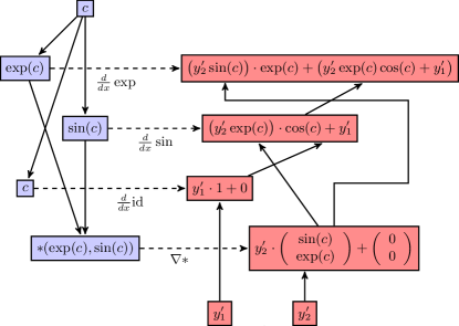
Figure 9: Computational graph for Example 9.1 with elements of $\mathbf{v}^{[4]}$ in blue and the evaluation of the directional derivative in red.

Figure 10: Minimal (not optimal!) F# example, similar to work in the library DiffSharp [10], [11], showing the implementation of the Reverse Mode for Example 9.1 with the test case $c=5$, $\mathbf{\overset{\leftharpoonup}{y}}=(1\ 1)$. (An optimal version would account for fan-out at each node.)

We summarize:

Theorem 9.2.

By the above, given $\mathbf{c}\in X\subset\mathbb{R}^{n}$ and $\mathbf{\overset{\leftharpoonup}{y}}\in\mathbb{R}^{1\times m}$, the evaluation of $\mathbf{\overset{\leftharpoonup}{y}}\cdot J_{f}(\mathbf{c})$ for an automatically differentiable function $f:X\to\mathbb{R}^{m}$ can be achieved by computing the vectors $\mathbf{\mathbf{v}}^{[0]},...,\mathbf{\mathbf{v}}^{[\mu]}$ and $\mathbf{\overline{v}}^{[\mu]},...,\mathbf{\overline{v}}^{[0]}$, where the computation of each $\mathbf{\overline{v}}^{[i-1]}$ is effectively the computation of the real numbers

$$\mathbf{\overline{v}}^{[i]}_{n+i}\cdot\frac{\partial\varphi_{i}}{\partial v_{k}}(v_{i_{1}}(\mathbf{c}),...,v_{i_{n_{i}}}(\mathbf{c}))+\mathbf{\overline{v}}^{[i]}_{k},\ \ \ k\neq n+i,$$

and $$\mathbf{\overline{v}}^{[i]}_{n+i}\cdot\frac{\partial\varphi_{i}}{\partial v_{n+i}}(v_{i_{1}}(\mathbf{c}),...,v_{i_{n_{i}}}(\mathbf{c})).$$

Comparing the complexity of Reverse AD with the one of symbolic differentiation for the examples given in Section 5 gives similar results as the comparison of Forward AD with symbolic differentiation. (See, for example, Figure 2 for the case of a composition of $3$ uni-variate functions.)

Acknowledgements: I like to thank Felix Filozov for his advice and his help with the code in Figure 6, Atılım Güneş Baydin for his advice and his help with the code in Figure 10 and Barak Pearlmutter for general valuable advice. I am further very thankful to the anonymous referees for valuable criticism and suggestions which led to a significant improvement of this paper.  

Funding: This work was supported by Science Foundation Ireland grant
09/IN.1/I2637.

 

Philipp Hoffmann
National University of Ireland, Maynooth
Department of Computer Science
Maynooth, County Kildare
Ireland
email: philipp.hoffmann@cs.nuim.ie philip.hoffmann@maths.ucd.ie

9.1 Reverse AD as the Dual Concept of Forward AD

If $h:M\to N$ is a differentiable function between differentiable manifolds $M$ and $N$, $\mathbf{x}\in M$ and $T_{\mathbf{x}}M$, $T_{h(\mathbf{x})}N$ are the tangent spaces of $M$ and $N$ at $\mathbf{x}$ and $h(\mathbf{x})$, respectively, then the push-forward of $h$ at $\mathbf{x}$ is a mapping $d_{\mathbf{x}}h:T_{\mathbf{x}}M\to T_{h(\mathbf{x})}N$. Its dual mapping (or transpose) is called the pull-back of $h$ at $\mathbf{x}$ and is the unique mapping

$$d^{*}_{\mathbf{x}}h:T^{*}_{h(\mathbf{x})}N\to T^{*}_{\mathbf{x}}M,\ \ \ \textrm{with}\ \ d^{*}_{\mathbf{x}}h(\mathbf{\overset{\leftharpoonup}{y}})=\mathbf{\overset{\leftharpoonup}{y}}\circ d_{\mathbf{x}}h,\ \ \forall\ \mathbf{\overset{\leftharpoonup}{y}}\in T^{*}_{h(\mathbf{x})}N,$$

where $T^{*}_{h(\mathbf{x})}N,T^{*}_{\mathbf{x}}M$ are the dual spaces of $T_{\mathbf{x}}M$ and $T_{h(\mathbf{x})}N$, respectively.

As mentioned in Section 7, in our case of a differentiable $f:X\to\mathbb{R}^{m}$ on open $X\subset\mathbb{R}^{n}$, the push-forward of $f$ at $\mathbf{x}\in X$, is given by $d_{\mathbf{x}}f(\mathbf{\overset{\rightharpoonup}{x}})=J_{f}(\mathbf{x})\cdot\mathbf{\overset{\rightharpoonup}{x}}$ for all $\mathbf{\overset{\rightharpoonup}{x}}\in\mathbb{R}^{n}$ and is, hence, a mapping $d_{\mathbf{x}}f$ from $\mathbb{R}^{n}$ to $\mathbb{R}^{m}$. The pull-back of $f$ at $\mathbf{x}$ then has to be a mapping $d^{*}_{\mathbf{x}}f:\mathbb{R}^{1\times m}\to\mathbb{R}^{1\times n}$ and has to be given by the matrix product

$$d^{*}_{\mathbf{x}}f(\mathbf{\overset{\leftharpoonup}{y}})=\mathbf{\overset{\leftharpoonup}{y}}\cdot J_{f}(\mathbf{x}),\ \ \forall\ \mathbf{\overset{\leftharpoonup}{y}}\in\mathbb{R}^{1\times m}.$$

Indeed, since matrix multiplication is associative, given $\mathbf{x}$, we have trivially

$$\left(\mathbf{\overset{\leftharpoonup}{y}}\circ d_{\mathbf{x}}f\right)(\mathbf{\overset{\rightharpoonup}{x}})=\mathbf{\overset{\leftharpoonup}{y}}\cdot\left(J_{f}(\mathbf{x})\cdot\mathbf{\overset{\rightharpoonup}{x}}\right)=\left(\mathbf{\overset{\leftharpoonup}{y}}\cdot J_{f}(\mathbf{x})\right)\cdot\mathbf{\overset{\rightharpoonup}{x}}=\left(d^{*}_{\mathbf{x}}h(\mathbf{\overset{\leftharpoonup}{y}})\right)(\mathbf{\overset{\rightharpoonup}{x}}),$$

for all $\mathbf{\overset{\leftharpoonup}{y}}\in\mathbb{R}^{1\times m},\mathbf{\overset{\rightharpoonup}{x}}\in\mathbb{R}^{n}$.

That is, the vector $\mathbf{\overset{\leftharpoonup}{y}}\cdot J_{f}(\mathbf{c})$ computed by the Reverse Mode of AD is the pull-back of $f$ at $\mathbf{c}\in X$ applied to $\mathbf{\overset{\leftharpoonup}{y}}$.

Hence, while one can define Forward AD in a general differential geometric setting as the application of the push-forward of $h$ to $(\mathbf{c},\mathbf{\overset{\rightharpoonup}{x}})\in TM$, Reverse AD may be defined as the computation of the pull-back of $h$ at $\mathbf{c}\in M$ applied to $\mathbf{\overset{\leftharpoonup}{y}}\in T^{*}_{h(\mathbf{c})}N$.

References

[1] M. Berz, Differential algebraic description of beam dynamics to very high orders, Particle Accelerators 24 (1989),
109–124.
[2] C. H. Bischof. On the Automatic Differentiation of Computer Programs and an Application to Multibody Systems,
IUTAM Symposium on Optimization of Mechanical Systems Solid Mechanics and its Applications 43 (1996),
41–48.
[3] W. K. Clifford, Preliminary Sketch of Bi-quaternions, Proceedings of the London Mathematical Society 4 (1873), 381–395.
[4] L. Dixon, Automatic Differentiation: Calculation of the Hessian, In: Encyclopedia of Optimization, second edition, Springer Science+Business Media, LLC., 2009, 133–137.
[5] V. Garczynski, Remarks on differential algebraic approach to particle beam optics by M. Berz, Nuclear Instruments and Methods in Physics Research Section A, 334 (2-3) (1993), 294–298.
[6] R. M. Gower, M. P. Mello, A new framework for the computation of Hessians, Optimization Methods and Software
27 (2) (2012), 251–273.
[7] A. Griewank, Achieving Logarithmic Growth of Temporal and Spatial Complexity in Reverse Automatic Differentiation,
Optimization Methods and Software 1 (1992), 35–54.
[8] A. Griewank, A Mathematical View of Automatic Differentiation, Acta Numerica 12 (2003), 321–398.
[9] A. Griewank and A. Walther, Evaluating Derivatives: Principles and Techniques of Algorithmic Differentiation, second edition, SIAM, Philadelphia, PA, 2008.
[10] A. G. Baydin, B. A. Pearlmutter, DiffSharp: Automatic Differentiation Library, version of 17th June 2015, http://diffsharp.github.io/DiffSharp/.
[11] A. G. Baydin, B. A. Pearlmutter, A. A. Radul, J. M. Siskind, Automatic differentiation and machine learning: a survey. arXiv preprint. arXiv:1502.05767 (2015).
[12] J. H. Hubbard and B. E. Lundell, A First Look at Differential Algebra, American Mathematical Monthly 118 (3) (2011), 245–261.
[13] F. John, Partial Differential Equations, second edition, Springer-Verlag, New York-Heidelberg-Berlin, 1975.
[15] J. Karczmarczuk, Functional Coding of Differential Forms, Proc First Scottish Workshop on Functional Programming, Stirling, Scotland, 1999.
[16] J. Karczmarczuk, Functional Differentiation of Computer Programs, Proc of the III ACM SIGPLAN International Conference on Functional Programming, Baltimore, MD, 1998, 195–203.
[17] J. Karczmarczuk, Functional Differentiation of Computer Programs, Higher-Order and Symbolic Computation
14 (1) (2001), 35–57.
[18] S. Lang, Introduction to Differentiable Manifolds, second edition, Springer-Verlag, New York-Heidelberg-Berlin, 2002.
[19] O. Manzyuk, A Simply Typed -Calculus of Forward Automatic Differentiation, Electronic Notes in Theoretical Computer Science 286 (2012), 257–272.
[20] B. A. Pearlmutter and J. M. Siskind, Lazy Multivariate Higher-Order Forward-Mode AD,
Proc of the 2007 Symposium on Principles of Programming Languages, Nice, France, 2007, 155–160.
[21] B. A. Pearlmutter and J. M. Siskind, Reverse-Mode AD in a Functional Framework: Lambda the Ultimate Backpropagator, TOPLAS 30 (2) (2008), 1–36.
[22] L. B. Rall, Differentiation and generation of Taylor coefficients in Pascal-SC, In: A New Approach to Scientific Computation, Academic Press, New York, 1983, 291–309.
[23] L. B. Rall, The Arithmetic of Differentiation, Mathematics Magazine 59, (1986), 275–282.
[24] J. Ritt, Differential Algebra, American Mathematical Society Colloquium Publications, vol. XXXIII, American Mathematical
Society, New York, 1950.
[25] J. M. Siskind and B. A. Pearlmutter, Nesting Forward-Mode AD in a Functional Framework, Higher-Order and Symbolic Computation 21 (4) (2008),361–376.
[26] R. Wengert, A Simple Automatic Derivative Evaluation Program, Communications of the ACM 7 (8) (1964), 463–464.