Constraining neutrino electromagnetic properties by germanium detectors

Abstract

The electromagnetic properties of neutrinos, which are either trivial or negligible in the context of the Standard Model, can probe new physics and have significant implications in astrophysics and cosmology. The current best direct limits on the neutrino millicharges and magnetic moments are both derived from data taken with germanium detectors with low thresholds at keV levels. In this paper, we discuss in detail a robust, ab initio method: the multiconfiguration relativistic random phase approximation, that enables us to reliably understand the germanium detector response at the sub-keV level, where atomic many-body physics matters. Using existing data with sub-keV thresholds, limits on reactor antineutrino’s millicharge, magnetic moment, and charge radius squared are derived. The projected sensitivities for next generation experiments are also given and discussed.

I Introduction

Investigations of neutrino properties continue to be an accretive field of emerging interests to both theoretical and experimental physicists. Their nonzero masses, as suggested by neutrino oscillation experiments with various sources, already hint the necessity of extending the Standard Model (SM) to accommodate massive neutrinos. It is no wonder that their properties such as absolute masses, mass hierarchy, Dirac or Majorana nature, and precise mixing parameters are among the most actively pursued topics in neutrino physics for their great discovery potential.

Another interesting venue to look for surprises in neutrinos is their nontrivial electromagnetic (EM) properties (see, e.g., Giunti and Studenikin (2014); *Broggini:2012df; *Wong:2005pa for recent reviews). In the SM, neutrinos are strictly neutral. Their tiny charge radii squared, magnetic dipole moments, anapole moments (require parity violation in addition), and electric dipole moments (require both parity and time-reversal violation in addition) only arise in forms of radiative corrections (in some cases, finite mass terms and flavor mixing matrix have to be included). Going beyond the SM, there are numerous conjectures of larger neutrino EM moments, including neutrinos being millicharged. The present best upper limits on some of these moments, either set directly by experiments, or inferred indirectly from observational evidences combined with theoretical arguments, are orders of magnitude larger than the SM predictions (see Olive et al. (2014) and references therein for the current status). As a result, this leaves space for new physics. Also, the additional EM interactions with the copious amount of neutrinos in the universe will have significant implications for astrophysics and cosmology.

It was recently identified Wong et al. (2010); Chen et al. (2014a) that the unexplored interaction channel of neutrino-induced atomic ionization:

$$\nu+\mathrm{A}\rightarrow\nu+\mathrm{A}^{-}+e^{-}\,,$$

is an interesting avenue to study possible neutrino electromagnetic effects, and has the potentials of producing surprises. The germanium atom (Ge) is selected for the studies, since there are matured Ge detector techniques with low (at the atomic transition range of keV) threshold and good resolution to resolve possible spectra structures and peaks and end-points, which are essential to provide smoking-gun positive signatures. Existing data from the TEXONO and GEMMA experiments with reactor neutrinos already provide bounds on neutrino magnetic moments Li et al. (2003); Wong et al. (2007); Beda et al. (2012, 2013), neutrino charge radius Deniz et al. (2010), and milli-charges Gninenko et al. (2007); Studenikin (2013). New generations of Ge detectors capable of measuring events as low as 100 eV are expected to further expand the sensitivities Lin et al. (2009); Li et al. (2013); Zhao et al. (2013); Agnese et al. (2014).

To interpret experimental data and put limits on these moments, an important theoretical input: the differential cross section formulae for neutrino scattering in detectors, is necessary (see, e.g., Ref. Kouzakov and Studenikin (2014) for a recent review of neutrino-atom collision theory). While the conventional approach of treating the atomic electrons as free particles is considered a good approximation at high energies, at sub-keV regime, which is similar to atomic scales, proper treatments of many-electron dynamics in atomic ionization must be incorporated for a better understanding of detector responses at low energies.

Motivated by this goal, we recently applied ab initio calculations in the framework of multiconfiguration relativistic random phase approximation (MCRRPA) theory to study the atomic ionization of germanium by neutrino scattering. Partial results were reported in Chen et al. (2014b) and Chen et al. (2014a), which dealt with the neutrino magnetic moment and millicharge, respectively.

The purpose of this article is twofold: On the theory part, we present our approach in full details, elaborate in particular the benchmark calculations that serve as a concrete basis on which the method and uncertainty estimate can be justified, and consider all observables that can be probed by atomic ionization. Comparisons with previous works  Fayans et al. (1992); Kopeikin et al. (1997); Fayans et al. (2001); Kopeikin et al. (2003); Wong et al. (2010); Voloshin (2010); Kouzakov and Studenikin (2011); Kouzakov et al. (2011) are given so that differences in various approaches and the applicability of various approximation schemes at the sub-keV regime can be clearly examined.

The organization of this paper is as follows. In Section II, we give the general formulation of atomic ionization by neutrinos, and mention two widely-used approximation schemes: free electron approximation and equivalent photon approximation in II.1 and II.2, respectively. Our approach to atomic many-body problems: the multiconfiguration relativistic random phase approximation, is outlined in Section III.1, and its application to the structure and photoionization of germanium atoms are described in Section III.2 and III.3, subsequently. In Section IV.1, we present and discuss our results for germanium ionization by neutrino scattering, and compare with existing works. Limits on neutrino electromagnetic moments are derived in Section IV.2 by using realistic reactor antineutrino spectra and data. As there have been proposals of using neutrinos from tritium $\beta$ decay to study neutrino magnetic moment Kopeikin et al. (2003); Giomataris and Vergados (2004); McLaughlin and Volpe (2004), our calculation for this case is presented in Section IV.3. The summary is in Section V, and the technical details of multipole expansion, which is relevant to our calculations, is in Appendix A.

II Formulation of Atomic Ionization by Neutrinos

Consider the ionization of an atom A by scattering a neutrino $\nu_{l}$ ($l$ denoting the flavor eigenstate) off atomic bound electrons

$$\nu_{l}+\mathrm{A}\rightarrow\nu_{l}+\mathrm{A}^{+}+e^{-}\,.$$ (1)

For $l=\mu,\tau$, the process only proceeds through the neutral weak interaction (in $t$-channel), while for $l=e$, the charged weak interaction (in $s$-channel) also contributes. Using a Feirz reordering, the general low-energy weak scattering amplitude can be compactly gathered in one formula

$$\mathcal{M}^{(w)}=\frac{G_{F}}{\sqrt{2}}j_{\mu}^{(w)}(c_{V}\mathcal{J}^{\mu}-c_{A}\mathcal{J}_{5}^{\mu})\,,$$ (2)

where $G_{F}$ is the Fermi constant. The neutrino weak current

$$j_{\mu}^{(w)}=\bar{\nu}(k_{2},s_{2})\gamma_{\mu}(1-\gamma_{5})\nu(k_{1},s_{1})\,,$$ (3)

takes on the usual Dirac bilinear form with $k_{1}=(\omega_{1},\vec{k_{1}})$, $k_{2}=(\omega_{2},\vec{k_{2}})$ being the four-momenta and $s_{1}$, $s_{2}$ being the helicity states of the neutrino before and after scattering, respectively. The energy and 3-momentum transfer by the neutrinos are defined as

$$q^{\mu}=(T,\vec{q})=(\omega_{1}-\omega_{2},\vec{k}_{1}-\vec{k}_{2})\,.$$ (4)

The atomic (axial-)vector current, $\mathcal{J}_{(5)}^{\mu}$,

$$\mathcal{J}_{(5)}^{\mu}\equiv\braket{\Psi_{f}}{\hat{\mathcal{J}}_{(5)}^{\mu}(-\vec{q})}{\Psi_{i}}=\int d^{3}x\,e^{i\vec{q}\cdot\vec{x}}\braket{\Psi_{f}}{\hat{\bar{\psi}}_{e}(\vec{x})\gamma^{\mu}(\gamma_{5})\hat{\psi}_{e}(\vec{x})}{\Psi_{i}}\,,$$ (5)

is the matrix element of a one-electron (axial-)vector current operator $\hat{\mathcal{J}}_{(5)}^{\mu}(-\vec{q})$ (in momentum space) evaluated with many-body atomic initial and final states, $\ket{\Psi_{i}}$ and $\ket{\Psi_{f}}$. The vector and axial-vector coupling constants are

$$c_{V}=-\frac{1}{2}+2\sin^{2}\theta_{w}+\delta_{l,e}\,, \qquad c_{A}=-\frac{1}{2}+\delta_{l,e}\,,$$ (6)

where $\theta_{w}$ is the Weinberg angle. The extra Kronecker delta is added to account for the additional $s$-channel scattering for $\nu_{e}$.

Now suppose a neutrino has nonzero electromagnetic (EM) moments; in the most general case, the associated EM current can be expressed as

$$j_{\mu}^{(\gamma)}= \bar{\nu}(k_{2},s_{2})\left[F_{1}(q^{2})\gamma_{\mu}-i(F_{2}(q^{2})+iF_{E}(q^{2})\gamma_{5})\sigma_{\mu\nu}q^{\nu}+F_{A}(q^{2})(q^{2}\gamma_{\mu}-\not{q}q_{\mu})\gamma_{5}\right]\nu(k_{1},s_{1})$$ (7)

where $q^{2}\equiv q_{\mu}q^{\mu}$. The four terms $F_{1}(q^{2})$, $F_{2}(q^{2})$, $F_{A}(q^{2})$, and $F_{E}(q^{2})$ are referred as the charge, anomalous magnetic, anapole, and electric dipole form factors, respectively. Up to the order of $q^{2}$ in $j_{\mu}^{(\gamma)}$, we define the electric charge, charge radius squared, magnetic dipole moment, anapole moment, and electric dipole moment of a neutrino by

$$\mathbbm{q}_{\nu} =F_{1}(0)\,,$$

$$\braket{\mathbbm{r}_{\nu}^{2}} =\left.6\frac{d}{dq^{2}}F_{1}(q^{2})\right|_{q^{2}\rightarrow 0}\,,$$

$$\bbkappa_{\nu} =F_{2}(0)\,,$$

$$\mathbbm{a}_{\nu} =F_{A}(0)\,,$$

$$\mathbbm{d}_{\nu} =F_{E}(0)\,,$$ (8)

respectively, and they are all measured in the fundamental charge units $e$. Note that the existence of $\mathbbm{a}_{\nu}$ violates parity conservation, and $\mathbbm{d}_{\nu}$ violates both parity and time-reversal conservation. Also, in the Standard Model, the values of both $\braket{\mathbbm{r}_{\nu}^{2}}$ and $\mathbbm{a}_{\nu}$ arising from electroweak radiative corrections are not gauge-independent quantities; only after the full radiative corrections being considered are the gauge-independent, physical observables resulted in Musolf and Holstein (1991). While there are attempts to define these moments in gauge-independent manners, but still controversial. Here we do not concern ourselves further with such subtleties, but just practically assume these exotic moments, whose definitions are consistent with current conservation as obviously seen in Eq. (7), exist, and study their contributions in scattering processes.

Any nonzero EM moments of a neutrino therefore generate additional contributions to the atomic ionization process; they are given by the associated EM scattering amplitude 

$$\mathcal{M}^{(\gamma)}=\frac{4\pi\alpha}{q^{2}}j_{\mu}^{(\gamma)}\mathcal{J}^{\mu}\,.$$ (9)

Before presenting the complete scattering formula, we discuss a few kinematical considerations that help to reduce the full result to a simpler form.

First, as neutrinos are much lighter than all the energy scales relevant to the atomic ionization processes of concern, an ultrarelativistic limit $m_{\nu}\rightarrow 0$ is considered a good approximation. In such cases, the chirality and helicity states of a neutrino are the same, so scattering amplitudes of neutrino-helicity-flipping interactions with $\bbkappa_{\nu}$ and $\mathbbm{d}_{\nu}$, do not interfere with ones of neutrino-helicity-conserving interactions. On the other hand, since weak interactions and those with $\mathbbm{q}_{\nu}$, $\braket{\mathbbm{r}_{\nu}^{2}}$, and $\mathbbm{a}_{\nu}$ all preserve helicity, there are interference terms between the weak and EM amplitudes. Their magnitudes are important when constraints of $\mathbbm{q}_{\nu}$, $\braket{\mathbbm{r}_{\nu}^{2}}$, and $\mathbbm{a}_{\nu}$ are to be extracted from experimental data.

Second, the interaction with $\braket{\mathbbm{r}_{\nu}^{2}}$ apparently takes a four-Fermi contact form (evidenced by the $1/q^{2}$ photon propagator being cancelled by the $q^{2}$ factor in the associated current), and so does the interaction with $\mathbbm{a}_{\nu}$ Musolf and Holstein (1991). As a result, the combined EM scattering amplitude

$$\mathcal{M}^{(\braket{\mathbbm{r}_{\nu}^{2}}+\mathbbm{a}_{\nu})}=4\pi\alpha[\bar{\nu}\gamma_{\mu}(\nicefrac{{1}}{{6}}\braket{\mathbbm{r}_{\nu}^{2}}+\mathbbm{a}_{\nu}\gamma_{5})\nu]\mathcal{J}^{\mu}\,,$$ (10)

look similar to $\mathcal{M}^{(w)}$, except no coupling to the atomic axial-vector current $\mathcal{J}_{5}^{\mu}$.

Third, by the identities

$$\bar{\nu}_{L}\gamma_{\mu}\nu_{L}=-\bar{\nu}_{L}\gamma_{\mu}\gamma_{5}\nu_{L}\,,\quad\bar{\nu}_{R}\sigma_{\mu\nu}\nu_{L}=-\bar{\nu}_{R}\sigma_{\mu\nu}\gamma_{5}\nu_{L}\,,$$ (11)

one deduces that $\braket{\gamma_{\nu}^{2}}$ and $a_{\nu}$ can not be distinguished in ultrarelativistic neutrino scattering and should effectively appear as one moment, the effective charge radius squared:

$$\braket{\mathbbm{r}_{\nu}^{2}}^{(\mathrm{eff})}=\braket{\mathbbm{r}_{\nu}^{2}}-6\mathbbm{a}_{\nu}\,.$$ (12)

The same argument applies to $\kappa_{\nu}$ and $d_{\nu}$ that they appear as one effective anomalous magnetic moment:

$$\bbkappa_{\nu}^{(\mathrm{eff})}=\bbkappa_{\nu}-i\mathbbm{d}_{\nu}\,.$$ (13)

Starting from the total scattering amplitude, $\mathcal{M}^{(w)}+\mathcal{M}^{(\gamma)}$, and following the standard procedure, the single differential cross section with respect to neutrino energy deposit $T$ for an inclusive process with a unpolarized target is obtained. When there is only weak scattering, the result is

$$\dfrac{d\sigma^{(w)}}{dT} = \dfrac{G_{F}^{2}}{\pi}(E_{\nu}-T)^{2}\int d\cos\theta\,\cos^{2}\dfrac{\theta}{2}\Big{\{}R_{00}^{(w)}-\dfrac{T}{|\vec{q}|}R_{03+30}^{(w)}+\dfrac{T^{2}}{|\vec{q}|^{2}}R_{33}^{(w)}$$ (14)

$$+ \left(\tan^{2}\dfrac{\theta}{2}-\dfrac{q^{2}}{2|\vec{q}|^{2}}\right)R_{11+22}^{(w)}+\tan\dfrac{\theta}{2}\sqrt{\tan^{2}\dfrac{\theta}{2}-\dfrac{q^{2}}{|\vec{q}|^{2}}}R_{12+21}^{(w)}\Big{\}}$$

where $\theta$ is the neutrino scattering angle, $E_{\nu}$ is the incident neutrino energy. The atomic weak response functions

$$R_{\mu\nu}^{(w)} = \frac{1}{2J_{i}+1}\sum_{M_{J_{i}}}\sum_{f}\braket{\Psi_{f}}{c_{V}\hat{\mathcal{J}}_{\mu}-c_{A}\hat{\mathcal{J}}_{5\mu}}{\Psi_{i}}\braket{\Psi_{f}}{c_{V}\hat{\mathcal{J}}_{\nu}-c_{A}\hat{\mathcal{J}}_{5\nu}}{\Psi_{i}}^{*}$$ (15)

$$\times\delta(T+E_{i}-E_{f})\,,$$

involve a sum of the final scattering states $\ket{\Psi_{f}}$ and a spin average of the initial states $\ket{\Psi_{i}}=\ket{J_{i},M_{J_{i}},\ldots}$, and the Dirac delta function imposes energy conservation. The Greek indices $\mu,\nu$ take values $0,1,2,3$, and without loss of generality, the direction of $\vec{q}$ is taken to be the quantization axis with $\mu=3$.

The contributions from the helicity-conserving (h.c.) interactions with $\mathbbm{q}_{\nu}$ and $\braket{\mathbbm{r}_{\nu}}^{\mathrm{(eff)}}$, as they interfere with the weak scattering, can be compactly included by the following substitution

$$\frac{d\sigma^{(w)}}{dT}\rightarrow\frac{d\sigma^{(\mathrm{h.c.})}}{dT}\,, \quad\mathrm{with}\,c_{V}\rightarrow c_{V}+2\sqrt{2}\pi\frac{\alpha}{G_{F}}(\frac{1}{q^{2}}\mathbbm{q}_{\nu}^{2}+\frac{1}{6}\braket{\mathbbm{r}_{\nu}^{2}}^{(\mathrm{eff})})\,.$$ (16)

It should be pointed out that the inclusion of $\mathbbm{q}_{\nu}$ is only formally, as it goes with a kinematics-dependent term $1/q^{2}$ that differentiates its contribution from the other contact interactions.

As will be explicitly shown later, the contribution from $\mathbbm{q}_{\nu}$ with the current upper limit $\lesssim 10^{-12}$ derived from direct measurements dominates over the weak scattering. When the $\mathbbm{q}_{\nu}$-weak interference terms are much less important, it is convenient to isolate the pure Coulomb (coul) scattering part,

$$\dfrac{d\sigma^{(\mathrm{coul})}}{dT} =\mathbbm{q}_{\nu}^{2} (2\pi\alpha^{2})\left(1-\frac{T}{E_{\nu}}\right)\int d\cos\theta\,\Big{\{}\dfrac{(2E_{\nu}-T)^{2}-|\vec{q}|^{2}}{|\vec{q}|{}^{4}}R_{00}^{(\gamma)}$$ (17)

$$- \left[\dfrac{q^{2}+4E_{\nu}(E_{\nu}-T)}{2|\vec{q}|^{2}q^{2}}+\dfrac{1}{q^{2}}\right]R_{11+22}^{(\gamma)}\Big{\}}\,,$$

which is proportional to $\mathbbm{q}_{\nu}^{2}$. In such cases, we apply the approximated form

$$\left.\frac{d\sigma^{(\mathrm{h.c.})}}{dT}\right|_{\mathrm{large\,}\mathbbm{q}_{\nu}}\approx\left.\frac{d\sigma^{(\mathrm{h.c.})}}{dT}\right|_{c_{V}\rightarrow c_{V}+\frac{\sqrt{2}\pi\alpha}{3G_{F}}\braket{\mathbbm{r}_{\nu}^{2}}^{(\mathrm{eff})}}+\frac{d\sigma^{(\mathrm{coul})}}{dT}\,.$$ (18)

On the other hand, the contribution from the the helicity-violating (h.v.) interaction with $\bbkappa_{\nu}^{(\mathrm{eff})}$ has no interference with the helicity-conserving part so that

$$\dfrac{d\sigma}{dT} =\dfrac{d\sigma^{(\mathrm{h.c.})}}{dT}+\dfrac{d\sigma^{(\mathrm{h.v.})}}{dT}\,,$$ (19)

with

$$\dfrac{d\sigma^{(\mathrm{h.v.})}}{dT} = (\bbkappa_{\nu}^{2}+\mathbbm{d}_{\nu}^{2})(2\pi\alpha^{2})\left(1-\frac{T}{E_{\nu}}\right)\int d\cos\theta\,\Big{\{}-\dfrac{(2E_{\nu}-T)^{2}q^{2}}{|\vec{q}|{}^{4}}\,R_{00}^{(\gamma)}$$ (20)

$$+\dfrac{q^{2}+4E_{\nu}(E_{\nu}-T)}{2|\vec{q}|^{2}}R_{11+22}^{(\gamma)}\Big{\}}\,.$$

Note that the EM response functions appearing in Eqs. (17) and (20) are related to the weak response functions by setting $c_{V}=1$ and $c_{A}=0$ in Eq. (15)

$$\left.R_{\mu\nu}^{(w)}\right|_{c_{V}=1,c_{A}=0}\rightarrow R_{\mu\nu}^{(\gamma)}\,,$$ (21)

as EM interactions only couple to vector currents (which result in $R_{12+21}^{(\gamma)}=0$). Because of vector current conservation, the longitudinal part of a spatial current density $(\mu=3)$ is related to the charge density ($\mu=0$). Therefore the response functions $R_{03+30}^{(\gamma)}$ and $R_{33}^{(\gamma)}$ are subsumed in $R_{00}^{(\gamma)}$ .

A couple of important remarks on kinematics in $\nicefrac{{d\sigma}}{{dT}}$ are due here: (i) For fixed $E_{\nu}$ and $T$, the square of four momentum transfer $q^{2}$ in the ultrarelativistic limit is determined by the neutrino scattering angle $\theta$

$$q^{2}=-4E_{\nu}^{2}\sin^{2}(\frac{\theta}{2})-m_{\nu}^{2}\frac{T^{2}}{E_{\nu}^{2}}\,.$$ (22)

It will not vanish even at the forward angle $\theta=0$ as long as the neutrino is not massless $m_{\nu}\neq 0$. (This is important for scattering with $\mathbbm{q}_{\nu}$). (ii) By four momentum conservation, the integration variable $\cos\theta$ is constrained by

$$\min\left\{1,\max\left[-1,\dfrac{E_{\nu}^{2}+(E_{\nu}-T)^{2}-2M_{\mathrm{A}}(T-B)}{2E_{\nu}(E_{\nu}-T)}\right]\right\}\leq\cos\theta\leq 1\,,$$ (23)

where $M_{\mathrm{A}}$ is the atomic mass and $B$ is the binding energy of the ejected electron.

To evaluate $\nicefrac{{d\sigma}}{{dT}}$, the most challenging task is the calculation of all relevant atomic response functions, Eqs.(15,21). Before discussing our ab initio approach in next section, we review a couple of simple approximation schemes that work in certain kinematic regimes and by which tedious many-body calculations can be spared.

II.1 Free Electron Approximation

In case of high energy scattering when electron binding energy is comparatively negligible, a conceptually straightforward approach is to use a neutrino-free-electron scattering formula $\nicefrac{{d\sigma^{(0)}}}{{dT}}$. The number of atomic electrons can be freed depends on the neutrino energy deposition $T$. By introducing a step function $\theta(T-B_{i})$ to judge whether the $i$th electron, with binding energy $B_{i}$, can contribute to the scattering process, one obtains the conventional scattering formula based on the free electron approximation

$$\left.\dfrac{d\sigma}{dT}\right|_{\mathrm{FEA}}=\sum_{i=1}^{Z}\theta(T-B_{i})\left.\dfrac{d\sigma^{(0)}}{dT}\right|_{q^{2}=-2m_{e}T}\,.$$ (24)

Despite FEA enjoys a lot of success in many situations, its applicability is not always self-evident, in particular when issues like relevant energy scales and kinematics of concern arise. For example, as it was shown explicitly in Ref. for hydrogen-like atoms: (i) The borderline incident neutrino energy above which FEA can apply is the binding momentum $\sim Zm_{e}\alpha$, instead of the binding energy $\sim Z^{2}m_{e}\alpha^{2}$. (ii) Because FEA only has a specific $q^{2}=-2m_{e}T$ in contrary to an allowed range prescribed by Eqs. (22,23) for the realistic case, it fails to be valid for relativistic muon scattering and nonrelativistic WIMP scattering. Therefore, to reduce the potential errors caused this conventional practice in particular for detector’s response at low energies is an important theoretical task.

II.2 Equivalent Photon Approximation

In typical EM scattering with ultrarelativistic charged particles, it was long established that the equivalent photon approximation (EPA) is well founded von Weizsacker (1934); Williams (1934); Greiner and Reinhardt (2009). Such processes mostly happen with peripheral scattering angles, i.e., $q^{2}\rightarrow 0$; it is thus obvious from Eq. (17) that the contribution from the transverse response function $R_{11+22}^{(\gamma)}$ dominates and the longitudinal part $R_{00}^{(\gamma)}$ can be ignored. As the “on-shell” transverse response function is directly linked to the total cross section of photoabsorption

$$\sigma_{\mathrm{abs}}^{(\gamma)}(T) =\dfrac{2\pi^{2}\alpha}{T}R_{11+22}^{(\gamma)}(q^{2}=0)\,,$$ (25)

the EPA further approximates $R_{11+22}^{(\gamma)}(q^{2})\approx R_{11+22}^{(\gamma)}(0)$ so that the Coulomb differential cross section for $\mathbbm{q}_{\nu}$

$$\left.\dfrac{d\sigma^{(\mathrm{coul})}}{dT}\right|_{\mathrm{EPA}} =-\mathbbm{q}_{\nu}^{2}(\frac{\alpha}{\pi})(1-\frac{T}{E_{\nu}})\sigma_{\mathrm{abs}}^{(\gamma)}(T)\int\,d\cos\theta\left[\dfrac{q^{2}+4E_{\nu}(E_{\nu}-T)}{2|\vec{q}|^{2}q^{2}}+\dfrac{1}{q^{2}}\right]\,,$$ (26)

can be directly determined by experiment.

Applying similar procedure to EM scattering with $\bbkappa_{\nu}$ and $\mathbbm{d}_{\nu}$:

$$\left.\dfrac{d\sigma^{(\mathrm{h.v.})}}{dT}\right|_{\mathrm{EPA}} =(\bbkappa_{\nu}^{2}+\mathbbm{d}_{\nu}^{2})(\frac{\alpha}{\pi})(1-\frac{T}{E_{\nu}})\sigma_{\mathrm{abs}}^{(\gamma)}(T)\int\,d\cos\theta\left[\dfrac{q^{2}+4E_{\nu}(E_{\nu}-T)}{2|\vec{q}|^{2}}\right]\,,$$ (27)

the cross section formula differs noticeably from the previous case by missing of the $1/q^{2}$ enhancement in the real photon limit. For more discussions about why there should not be atomic-enhanced sensitivities to neutrino magnetic moments at low energies, in contrary to what was claimed in Ref. Wong et al. (2010) (which is based on a slight different twist of Eq. 27), we refer readers to Refs. Voloshin (2010); Chen et al. (2013) for details.

III ab initio Description of Germanium

To go beyond the simple approximation schemes mentioned in the last section and evaluate the cross section formulae more reliably at low energies, the structure and ionization of detector atoms have to be considered on a more elaborate basis. In this section, we first introduce our approach to the atomic many-body problems: the multiconfiguration relativistic random phase approximation (MCRRPA) theory. In the following subsections, we present our results for the structure and photoionization of germanium atoms, respectively, and benchmark the quality of MCRRPA as reliable approach to describe the responses of germanium detectors.

III.1 The MCRRPA Theory

The relativistic random-phase approximation (RRPA) has been applied, with remarkable successes, to photoexcitation and photoionization of closed-shell atoms and ions of high nuclear charge, such as heavy noble gas atoms, where the ground state is well isolated from the excited states. For other closed-shell systems, such as alkaline-earth atoms, which have low-lying excited states, such applications have been less successful, owing to the importance of two-electron excitations which are omitted in the RRPA. The MCRRPA theory is a generalization RRPA by using a multiconfiguration wave function as the reference state which is suitable for treating photoexcitation and photoionization of closed-shell and certain open-shell systems of high nuclear charge. The great success it achieved in various atomic radiative processes can be found in Refs. Huang et al. (1995). A detailed formulation of the MCRRPA has been given in a previous paper Huang and Johnson (1982), and we summarize the essential features here.

One way to derive the MCRRPA equations is through linearizing the time-dependent multiconfiguration Hartree-Fock (TDHF) equations.  For a N-electron atomic system, the time-dependent relativistic Hamiltonian is given by

$$H(t)=H_{0}+V(t)\,,$$ (28)

where the unperturbed Hamiltonian

$$H_{0}={\displaystyle\sum_{i=1}^{N}h(\vec{r}_{i})+{\displaystyle\sum_{i<j}^{N}\dfrac{e^{2}}{r_{ij}}\,,}}$$ (29)

contains the sum of single-electron Dirac Hamiltonians

$$h(\vec{r})=c\vec{\alpha}\cdot\vec{p}+\beta c^{2}-\frac{Z}{r}\,,$$ (30)

and the Coulomb repulsion between two-electron pairs (the latter summation); and the time-dependent external perturbation

$$V(t)=\sum_{i=1}^{N}v_{+}(\vec{r}_{i})e^{-i\omega t}+\sum_{i=1}^{N}v_{-}(\vec{r}_{i})e^{+i\omega t}\,,$$ (31)

takes a harmonic form and induces transitions between atomic states. Note that atomic units (a.u.) are employed throughout this paper.

Let $\Phi(t)$ be the time-dependent solution of the wave equation

$$i\frac{\partial\Phi(t)}{\partial t}=H(t)\Phi(t)\,,$$ (32)

our point of departure to obtaining $\Phi(t)$ is through the time-dependent variational principle

$$\left<\delta\Phi(t)\left|\left[i\frac{\partial}{\partial t}-H(t)\right]\right|\Phi(t)\right>=0\,.$$ (33)

Without loss of generality, it is convenient to factor out from $\Phi(t)$ the phase due to the time-evolution of the stationary state of $H_{0}$

$$\Phi(t)=e^{-iEt}\Psi(t)\,,$$ (34)

with $E$ denoting the energy eigenvalue of $H_{0}$. As a result, the time-dependent variational principle is recast as

$$\left<\delta\Psi(t)\left|\left[E+i\frac{\partial}{\partial t}-H(t)\right]\right|\Psi(t)\right>=0\,.$$ (35)

For an atomic state with angular momentum JM and parity $\pi$, the multiconfiguration Hartree-Fock approximation assumes the wave function $\Psi(t)$ as a superposition of configuration wave functions $\psi_{a}(t)$ of the same JM and $\pi$, viz.

$$\Psi(t)={\displaystyle\sum_{a}C_{a}(t)\psi_{a}(t)\,,}$$ (36)

where a is a configuration index, and $C_{a}(t)$ are time-dependent weights. The configuration wave functions $\psi_{a}(t)$ are built up from one-electron orbitals $u_{\alpha}(t)$. To guarantee the normalization of $\Psi(t)$

$$\left<\Psi(t)|\Psi(t)\right>=1\,,$$ (37)

the following subsidiary conditions

$$\left<u_{\alpha}(t)|u_{\beta}(t)\right> =\delta_{\alpha\beta}\,,$$ (38)

$$\left<\psi_{a}(t)|\psi_{b}(t)\right> =\delta_{ab}\,,$$ (39)

$$\sum_{a}C_{a}^{\star}(t)C_{a}(t) =1\,,$$ (40)

are imposed. Since the perturbation $V(t)$ that induces atomic transitions is harmonic in time, both $C_{a}(t)$ and $u_{\alpha}(t)$ assume the following expansion

$$C_{a}(t)=C_{a}+\left[C_{a}\right]_{+}e^{-i\omega t}+\left[C_{a}\right]_{-}e^{+i\omega t}\ldots,$$ (41)

$$u_{\alpha}(t)=u_{\alpha}+w_{\alpha+}e^{-i\omega t}+w_{\alpha-}e^{+i\omega t}+\ldots,$$ (42)

where “$\ldots$” denotes higher harmonic responses.

Approximate time-dependent solution of Eq. (35) are thus obtained with the wave function, Eq. (36), constrained by Eqs. (37–42). The terms $C_{a}$ and $u_{\alpha}$, which are independent of the external field, lead to the usual stationary multiconfiguration Dirac-Fock (MCDF) description of an atomic state and this gives the initial state wave function $\ket{\Psi_{i}}$ of our problem. The terms $\left[C_{a}\right]_{\pm}$ and $w_{\alpha\pm}$, which are induced by the external field, lead to equations describing the linear response of the atomic state to the external field; these linear response equations are called the multiconfiguration relativistic random-phase approximation (MCRRPA) equations Huang and Johnson (1982); Johnson and Huang (1982). Furthermore, the incoming wave boundary condition is incorporated to yield the physical asymptotic Coulomb wave function that describes an outgoing continuum electron with a residual ion in the final state $\bra{\Psi_{f}}$ of our problem. Since the external perturbation $V(t)$ may have components with nonvanishing angular momentum and with odd parity, the atomic wave function contains terms of mixed angular momentum and parity. If one starts from a single-configuration reference state, the MCRRPA equations reduce to the usual RRPA equations.

To make connection with the general scattering formalism set up in the last section, we note that the perturbing field components $v_{\pm}$ take the matrix form

$$\left<\Psi_{f},\,E_{f}=E_{i}\pm\omega\left|v_{\pm}^{(w,\gamma)}\right|\Psi_{i}\right>=\left.\mathcal{M}^{(w,\gamma)}\right|_{E_{f}=E_{i}\pm\omega}\,,$$ (43)

and they cause atomic excitation and de-excitation by an energy quantum $\omega$, respectively. Therefore, in the process of solving the MCRRPA equations, the corresponding scattering amplitudes are simultaneously determined.

Another important point to mention in our implementation of the MCRRPA scheme is the choice of the spherical-wave basis. As a result, all transition operators are cast into spherical multipole operators. The key step in the spherical multipole expansion is breaking down the atomic charge density operator $\hat{\mathcal{J}^{0}}(-\vec{q})$ into a series of charge multipole operators $\hat{C}_{JM}$ , and the atomic 3-current density operator $\hat{\mathcal{J}}^{i}(-\vec{q})$ into a series of longitudinal $\hat{L}_{JM}$, transverse electric $\hat{E}_{JM}$, and transverse magnetic $\hat{M}_{JM}$ multipole operators, with $JM$ denoting the angular momentum quantum numbers. The advantages of such an implementation include: (i) The three-dimensional equation of motion for each orbital is reduced to a one-dimensional equation. (ii) Each multipole operator has its own angular momentum and parity selection rules, so the MCRRPA equations can be divided into smaller blocks in which numerical calculations can be performed more efficiently. (iii) For $1/|\vec{q}|$ larger than the size of the atom, the multipole expansion converges rapidly. For the axial charge $\hat{\mathcal{J}}_{5}^{0}(-\vec{q})$ and 3-current $\hat{\mathcal{J}}_{5}^{i}(-\vec{q})$, four more types of multipole operators $\hat{C}_{JM}^{5}$, $\hat{L}_{JM}^{5}$, $\hat{E}_{JM}^{5}$, and $\hat{M}_{JM}^{5}$, are to be introduced. Each of them has opposite parity selection rule compared to its vector counterpart. The details of the multipole expansion is given in Appendix A.

III.2 Atomic Structure of Germanium by MCDF

For the germanium atom, we chose the multiconfiguration reference state to be

$$\Psi=C_{1}\left(4p_{1/2}^{2}\right)_{0}+C_{2}\left(4p_{3/2}^{2}\right)_{0}\,,$$ (44)

a linear combination of two configurations with total angular momentum $J=0$ and parity $\pi=\mathrm{even}$, where the coefficients $C_{1}$ and $C_{2}$ are the configuration weights. The notation $\left(4l_{j}^{2}\right)$ denotes symbolically an anti-symmetrized wave function constructed from two electrons in the valence orbital $4l_{j}$. The rest of the electrons in the 10 inner orbitals $4s_{1/2}$, $3d_{5/2}$, $3d_{3/2}$, $3p_{3/2}$, $3p_{1/2}$, $3s_{1/2}$, $2p_{3/2}$, $2p_{1/2}$, , $2s_{1/2}$, and $1s_{1/2}$ form the closed core.

The ground-state wave function obeying the MCDF equations is solved by the computer code Desclaux (1975), which yields all the core and valence orbitals, and the configuration weights $C_{1}$ and $C_{2}$. In Table 1, all calculated orbital binding energies are shown and compared with the edge energies extracted from photoabsorption data of germanium solids (to be discussed in the next section). In Table 1, the configuration weights and their corresponding percentages are given.

Table 1: The binding energies (in eV) of the atomic germanium orbits from the present MCDF calculations. The experimental data are the edge energies extracted from photoabsorption data of germanium solids.

Label				MCDF		Exp.a
Subshell		Orbital
$N_{III}$		$4p_{1/2}$		7.8
$N_{II}$		$4p_{3/2}$		8.0
$N_{I}$		$4s_{1/2}$		15.4
$M_{V}$		$3d_{5/2}$		43.1		29.3
$M_{IV}$		$3d_{3/2}$		43.8		29.9
$M_{III}$		$3p_{3/2}$		140.1		120.8
$M_{II}$		$3p_{1/2}$		144.8		124.9
$M_{I}$		$3s_{1/2}$		201.5		180.1
$L_{III}$		$3p_{3/2}$		1255.6		1217.0
$L_{II}$		$3p_{1/2}$		1287.9		1248.1
$L_{I}$		$2s_{1/2}$		1454.4		1414.6
$K$		$1s_{1/2}$		11185.5		11103.1
aFrom Ref. Henke et al. (1993).

Table 2: Configuration weights of the germanium atom in its ground state ($J^{\pi}=0^{+}$) from the present MCDF calculations.

Valence Configuration		Configuration Weight		Percentage
$4p_{1/2}^{\,2}$		0.84939		72.15$\%$
$4p_{3/2}^{\,2}$		0.52776		27.85 $\%$

III.3 Photoabsorption of Germanium by MCRRPA

To further benchmark the MCRRPA method, in particular its applicability to the atomic bound-to-free transition of germanium, we consider the photoabsorption of germanium above the ionization threshold, for which experimental data are available.

In the multipole expansion scheme, an external perturbing field with parameters $J$ and $\lambda$ gives rise to one-particle-one-hole excitation channels which are restricted by the angular momentum and parity conservation. Suppose one of the atomic bound electron in the $nl_{j}$ orbital is promoted to a free continuum state $\epsilon l_{j^{\prime}}^{\prime}$ ($\epsilon$ denotes the kinetic energy) by this $J\lambda$ perturbing field, the relevant quantum numbers then satisfy the following selection rules:

$$\left|\,j-J\right|\,\leqslant\,j^{\prime}\,\leqslant\left|\,j+J\right|,\quad(\mathrm{Angular\>Momentum\>Selection\>Rule})$$ (45)

$$l+l^{\prime}+J+\lambda-1=\mathrm{even}.\quad(\mathrm{Parity\>Selection\>Rule})$$ (46)

As a result, in response to the multipole perturbations (with different $J\lambda$), the germanium atom (a many-body ${}^{1}S_{0}$ state) is excited to a state mixed with components of different total angular momenta and parities.

For example, consider the case arising from excitations of the two valence electrons in the valence orbitals $4p_{1/2}$ or $4p_{3/2}$. There are 5 possible excitation channels responding to the electric-type dipole excitation (by a $E_{J=1}$ operator):

$\qquad\qquad 4p_{1/2}\rightarrow\epsilon s_{1/2},$

$\qquad\qquad 4p_{1/2}\rightarrow\epsilon d_{3/2},$

$\qquad\qquad 4p_{3/2}\rightarrow\epsilon s_{1/2},$

$\qquad\qquad 4p_{3/2}\rightarrow\epsilon d_{3/2},$

$\qquad\qquad 4p_{3/2}\rightarrow\epsilon d_{5/2}.$

Besides the above valence-excitation channels, the 10 inner core orbitals give rise to additional 24 channels. In total, when one considers all possible excitations from all orbitals, there are 29 excitation channels to be taken into account in the electric-type dipole excitation. These 29 interacting jj-coupled channels are all included in our MCRRPA framework to account for the final ionic-state electron correlations. The corresponding MCRRPA equations comprise a system of coupled differential equations up to 29 channels with 116 unknown radial functions to be numerically solved in a self-consistent manner.

To obtain the total photoabsorption cross section, all electric-type ($E_{J}$) and magnetic-type ($M_{J}$) multipole excitations which contribute to the on-shell transverse response function, $R_{11+22}^{(\gamma)}(q^{2}=0)$, are summed. For photons with energy $T\lesssim 10\,\mathrm{keV}$, it is found that high-order multipole transition probabilities decrease rapidly in an exponential mode. We choose the cut-off value $J_{\mathrm{cut}}$ in the multipole expansion by the following recursive procedure: We first sum over the multipole transition probabilities up to a definite polarity order (which should be high enough so the rapidly-decreasing pattern starts to show), and extrapolate the corrections from succeeding higher multipoles by a proper exponential form. Then $J_{\mathrm{cut}}$ is fixed once the contributions from $\sum_{J>J_{\mathrm{cut}}}$ is estimated, by the exponential law, to be below 1% of the total from $\sum_{J\leq J_{\mathrm{cut}}}$.

In Fig. 1(a), the photoabsorption cross sections from the MCRRPA method and experimental data are shown for incident photon energies ranging from 10 eV to 10 keV. The MCRRPA results agree very well with experiments for photon energies larger than 80 eV, with errors uniformly below the $5\%$ level. The discrepancy below 80 eV is relatively large and we believe it is due to the fact that the experimental data were taken from solid-phase Ge targets, whose wave functions and orbital binding energies, in particular for outer-shell electrons, are affected by nearby atoms and therefore different from the ones of a single atom. As shown by Table 1 and Fig. 1(a), the solid effects are especially significant for the 3d orbitals. On the other hand, the inner-shell electrons are less affected by crystal structure; as a result, our calculation well-reproduces the data of photon energies $T\geq 100\,\mathrm{eV}$, where cross sections are dominated by ionization of inner-shell electrons. To estimate the degree to which our MCRRPA results will be affected by the solid effects in the $T\geq 100\,\mathrm{eV}$ region, we carried out a parallel calculation in which the theoretical ionization thresholds are artificially aligned with the experimental ones. The results, plotted in Fig. 1(b), show that the deviations from experimental data are still kept below the $10\%$ level. Therefore, we estimate the theoretical uncertainty due to the solid effects to be $\lesssim 10\%$ in the $T\geq 100\,\mathrm{eV}$ region.

Figure 1: Photoabsorption cross sections of Ge. The data are taken from Ref. Henke et al. (1993). The MCRRPA line in panel (a) shows our numerical results; the one in panel (b) is obtained by forcing all shell energies aligned to the experimental edge energies.

Summing up this section, we demonstrate that our MCRRPA approach is capable of giving a good description of a germanium atom and its photoabsorption process with photon energy larger than 100 eV. In other words, the many-body wave functions, single particle basis states, and relevant transition matrix elements thus obtained should be good approximations to the exact answers. In the next section, we shall apply this approach to germanium ionization by neutrinos.

IV Ionization of Germanium by Neutrinos

As shown in Eqs. (14,17,20), ionization of germanium by neutrinos depends on various atomic response functions $R$’s, which need explicit many-body calculations. The only differences in calculating the response functions for this case from the ones for photoionization are (i) different atomic current operators are involved, and (ii) different kinematics are probed (the former are mostly off-shell, while the latter are purely on-shell). Therefore, it is straightforward to treat the problem in the MCRRPA framework simply by taking more types of multipole operators and their off-shellness into account. Both aspects are not expected to generate additional complexity or problems in many-body physics, therefore, one can take similar confidence on MCRRPA in this case as what has been acquired in the photoabsorption case with $T\geq 100\,\mathrm{eV}$.

Because $q^{2}$ in a $t$-channel scattering process is space-like, i.e., $q^{2}<0$ or $T^{2}<|\vec{q}|^{2}$, an off-shell current operator typically yields a multipole expansion which converges more slowly than its on-shell counterpart. Here we use an example to demonstrate a multipole expansion scheme is still valid and effective for the cases we are interested. Consider an incident neutrino with 1 MeV energy (a typical value for reactor antineutrinos) and depositing 1 keV energy to the detector through the charge-type multipole operators $\hat{C}_{JM}$ in weak, magnetic moment, or millicharge interactions. The contributions of $\hat{C}_{JM}$ to the differential cross sections $d\sigma/dT$ in these three cases are plotted in Fig. 2(a), (b), and (c), respectively. All these plots feature exponential decay behaviors with increasing multipolarity $J$, and they are fitted to be proportional to $e^{-0.15J}$, $e^{-0.14J}$, and $e^{-0.10J}$, respectively. Therefore, we can apply the same cutoff procedure mentioned in the last section in multipole expansions and control the higher-multipole uncertainty at the $1\%$ level. For the entire kinematics considered in this work, it is found that the cutoff values $J_{\mathrm{cut}}$ are no more than $50-60$.

Figure 2: Normalized contributions from the series of charge multipole operators $C_{J}$’s to differential cross sections for (a) weak interaction, (b) magnetic moment interaction, and (c) millicharge interaction. The incident neutrino has 1 MeV energy and deposits 1 keV energy.

IV.1 Results and Discussion

In this section, we present our calculated differential cross sections for germanium ionization with two representative incident neutrino energies: (a) $E_{\nu}=1\,\mathrm{MeV}$ and (b) $E_{\nu}=10\,\mathrm{keV}$. The former case is typical for reactor antineutrinos, while the latter case gives an example of very low energy neutrinos, e.g., ones from tritium $\beta$ decay.

IV.1.1 Weak Interaction

The differential cross sections due to the weak interaction, i.e., Eq. (14), are given in Fig. 3 (see also Fig. 2 in Ref. Chen et al. (2014b)). As shown in panel (a), our MCRRPA calculation and the conventional FEA scheme gradually converge when the energy transfer is larger than 1 keV. On the other hand, below $T=1\,\mathrm{keV},$ FEA starts to overestimate the differential cross sections. In other words, we found the atomic binding effect suppress the weak scattering cross sections at low energies in comparison to the free scattering picture. This conclusion is consistent with previous explicit many-body calculations Fayans et al. (1992); Kopeikin et al. (1997); Fayans et al. (2001); Kopeikin et al. (2003).

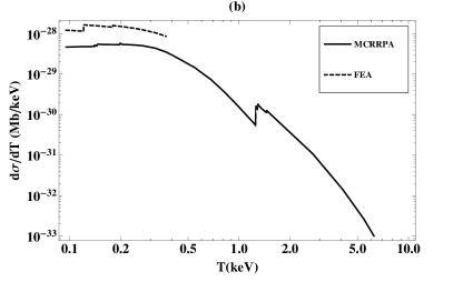
Figure 3: Differential cross sections for germanium ionization by neutrino weak interaction with neutrino incident energies (a) $E_{\nu}=$1 MeV and (b) $E_{\nu}=$ 10 keV. (See also Fig. 2 in Ref. Chen et al. (2014b))

In very low energy neutrino scattering, the FEA scheme has another severe problem that comes with its specific kinematic constrain: $q^{2}=-2m_{e}T$. This leads to a maximum energy transfer $T_{\mathrm{max}}\approx 0.38\,\mathrm{keV}$ for a 10-keV neutrino beam–as shown by the sharp cutoff for the FEA curve in panel (b); while there is no such cutoff expected in a neutrino–atom ionization process. Experiments with good energy resolution should be able to discern this difference.

IV.1.2 Magnetic Moment Interaction

The differential cross sections due to the interaction with $\bbkappa_{\nu}^{(\mathrm{eff})}$, i.e., Eq. (20), are given in Fig. 4 (see also Fig. 2 in Ref. Chen et al. (2014b)). The comparison of the MCRRPA and FEA results shows very similar features as the case of weak scattering: FEA overestimates in the $T\lesssim 1\,\mathrm{keV}$ region and gradually converges to MCRRPA for $T\gtrsim 1\,\mathrm{keV}$, and our conclusion in this case is also consistent with previous explicit many-body calculations Fayans et al. (1992); Kopeikin et al. (1997); Fayans et al. (2001); Kopeikin et al. (2003).

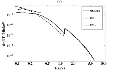
Figure 4: Differential cross sections for germanium ionization by neutrino magnetic moment interaction with neutrino incident energies (a) $E_{\nu}=$1 MeV and (b) $E_{\nu}=$ 10 keV, in units of $\bbkappa_{\nu}^{\mathrm{(eff)}2}$. (See also Fig. 2 in Ref. Chen et al. (2014b))

As there have been quite extensive recent discussions about the role of atomic structure in scattering by neutrino magnetic moments, we try to clarify the confusion which is caused by the applicabilities of various approximation schemes:

1. EPA: It was first claimed in Ref. Wong et al. (2010) that atomic structure can greatly enhance the sensitivity to $\bbkappa_{\nu}^{(\mathrm{eff})}$ by orders of magnitude than the FEA prediction in the $T<1\,\mathrm{keV}$ region for germanium. However, later works inspired by this, using various approaches, all came to the opposite conclusion Voloshin (2010); Kouzakov and Studenikin (2011); Kouzakov et al. (2011); Chen et al. (2014b). The source of the huge overestimation in Ref. Wong et al. (2010): the use of an unconventional EPA scheme, was pointed out in Ref. Chen et al. (2013) by considering a simple case of hydrogen atoms. Applying the same scheme to germanium, the results are shown by the EPA^∗ curves in Fig. 4. In panel (a), one clearly sees the orders-of-magnitude enhancement that EPA^∗ predicts. On the other hand, in panel (b), EPA^∗ does agree well with MCRRPA for $T>1\,\mathrm{keV}$. This is consistent with the feature pointed out in Ref. Chen et al. (2013): When incident neutrino energy (in this case, 10 keV) falls below the scale of atomic binding momentum (in this case, 35 keV for the most important $3p$ shell), the EPA^∗ works incidentally.

2. The Voloshin sum rules: Quantum-mechanical sum rules for neutrino weak and magnetic-moment scattering were derived by Voloshin Voloshin (2010) and refined in later works Kouzakov and Studenikin (2011); Kouzakov et al. (2011). Using several justified assumptions, the sum rules concluded that treating atomic electrons as free particles be a good approximation. One important step in these sum rules is extending the integration over $q^{2}$ (equivalent to integration over the neutrino scattering angle $\theta$ for a fixed $T$) from the physical range $[T^{2},4E_{\nu}^{2}]$ to $[0,\infty)$. In this sense, the sum-rule results, or equivalently the FEA results, can be interpreted as upper limits for realistic $d\sigma/dT$, and this is consistent with our MCRRPA curves being under the FEA ones in Figs. 3 and 4. However, the larger discrepancy between realistic calculations and FEA at sub-keV energies seems to be in contradiction with the sum-rule-FEA argument: With low $T$, only outer-shell electrons are ionized, so the sum rules should work even better, not worse, since these electrons are less bound, or closer to be free electrons. The main reason, as pointed out in Ref. Kouzakov and Studenikin (2014), is the missing of two-electron correlation in the sum rule derivation, which plays a more important role at low energies.

IV.1.3 Millicharge Interaction

The differential cross sections due to the interaction quadratic in $\mathbbm{q}_{\nu}$, i.e., Eq. (17), are given in Fig. 5. While the linear term due to the EM–weak interference can be calculated straightforwardly, it can be safely ignored at the current and projected sensitivity levels of direct experiments with $\mathbbm{q}_{\nu}\sim 10^{-12}-10^{-13}$.

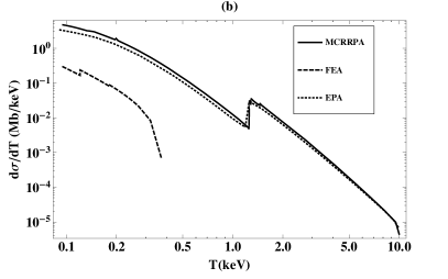
Figure 5: Differential cross sections for germanium ionization by neutrino millicharge interaction with neutrino incident energies (a) $E_{\nu}=$1 MeV and (b) $E_{\nu}=$ 10 keV, in units of $\mathbbm{q}_{\nu}^{2}$.

Unlike the previous two cases that FEA works well for neutrino weak and magnetic moment scattering with big enough incident energy $E_{\nu}$ and energy deposition $T$, it underestimates the millicharge scattering cross sections, in particular in the most interested sub-keV region of $T$. Instead, it is EPA that works much better in this case. The main reason, as pointed out in Ref. Chen et al. (2013), is due to the kinematic factor $1/q^{2}$ that goes along the transverse response function $R_{11+22}^{(\gamma)}$ in Eq. (17). This factor weights more the forward scattering region with $q^{2}\rightarrow 0$, where photons behave like real particles. For the same reason one can see that the FEA constraint: $q^{2}=-2m_{e}T$ deviates substantially from the true kinematics of this scattering process.

Because of the same $1/q^{2}$ factor, we also note that the differential cross section contains a logarithmic term $\log(E_{\nu}/m_{\nu})$, which diverges at the limit of massless neutrinos Chen et al. (2014a). While it is known that neutrinos are not massless, their masses have not been determined precisely yet. Instead of using the current upper limit $m_{\nu_{e}}<2\,\mathrm{eV}$ as the cutoff value in this logarithm to present our results in this paper, we adopt the Debye length of germanium solid: 0.68 $\mu\mathrm{m}$ which characterizes the scale of screen Coulomb interaction and acts like a 0.29 eV mass cutoff (a value also similar to the projected sensitivity on $m_{\nu_{e}}$ by the KATRIN experiment). The uncertainty in cross sections due to this one-order-of-magnitude difference in the mass cutoff is about $20\%$.

IV.1.4 Charge Radius Interaction

The differential cross sections due to the interaction with $\braket{\mathbbm{r}_{\nu}^{2}}^{(\mathrm{eff})}$, i.e., by taking $d\sigma^{(\mathrm{h.c.})}/dT-d\sigma^{(w)}/dT$ with $\mathbbm{q}_{\nu}=0$ in Eq. (16), are given in Fig. 6. Since the charge radius interaction takes the same contact form as the weak interaction, it is natural to expect the failure of the EPA scheme, so not shown in the figure. The main difference between the charge radius and weak interactions is that the former depends on the atomic vector-current response, while the latter on the atomic vector-minus-axial-vector-current (V-A) response. However, as can be seen from the comparison of Figs. 6 and 3, both differential cross sections share very similar $T$-dependence. The differences between the MCRRPA and FEA results are also similar to the case of weak scattering.

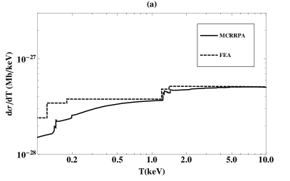
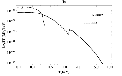
Figure 6: Differential cross sections for germanium ionization by neutrino charge radius interaction with neutrino incident energies (a) $E_{\nu}=$1 MeV and (b) $E_{\nu}=$ 10 keV, in units of $2c_{V}\rho+\rho^{2}$ and $\rho\equiv\frac{\sqrt{2}\pi}{3}\frac{\alpha}{G_{F}}\braket{\mathbbm{r}_{\nu}^{2}}^{(\mathrm{eff})}$.

IV.2 Reactor Antineutrinos

Existing data from reactor neutrino experiments using germanium ionization detectors Li et al. (2003); Wong et al. (2007); Beda et al. (2012, 2013) provide excellent platform to investigate the atomic ionization effects induced by neutrino electromagnetic interactions. The sensitivities depend on the detectable threshold of the differential cross section, as well as the neutrino flux but are mostly independent to the neutrino energy. Therefore, the enormous $\bar{\nu}_{e}$ flux (order of $10^{13}\,\mathrm{cm^{-2}\,s^{-1}}$, at a typical distance of $20\,\mathrm{m}$ from the reactor core) at the MeV-range energy from nuclear power reactors is a well-suited source. The germanium detectors, with their excellent energy resolution and sub-keV threshold, are ideal as means of studying these effects. The experimental features as peaks or edges at the definite $K$- and $L$-X-rays energies as well as with predictable intensity ratios provide potential smoking-gun signatures of these effects Wong et al. (2010); Chen et al. (2014a).

Denoting the reactor $\bar{\nu}_{e}$ spectrum by $\phi(E_{\nu})$, the measured differential spectra $\braket{d\sigma/dT}$ is related to the theoretical formulae of Eqs. 14, 17 and 20, via:

$$\left\langle\frac{d\sigma}{dT}\right\rangle=\frac{\int dE_{\nu}\,\phi(E_{\nu})\frac{d\sigma}{dT}(E_{\nu})}{\int dE_{\nu}\,\phi(E_{\nu})}\,.$$ (47)

The measurable spectra due to weak interactions, neutrino magnetic moments at $\bbkappa_{\nu}^{\mathrm{(eff)}}=10^{-11}\,\mu_{\mathrm{B}}$, milli-charges at $\mathbbm{q}_{\nu}=10^{-12}\,e$ and charge radius at $\braket{\mathbbm{r}_{\nu}^{2}}^{(\mathrm{eff})}=[6\times 10^{-3}\,\mathrm{fm}]^{2}$ at a reactor $\bar{\nu}_{e}$ flux of $10^{13}\,\mathrm{cm}^{-2}\,\mathrm{s}^{-1}$ are depicted in Fig. 7. These are compared with most sensitive data set from the TEXONO Li et al. (2003); Wong et al. (2007) and GEMMA Beda et al. (2012, 2013) experiments and the corresponding limits at 90% CL are listed in Table IV.2. Standard algorithms were adopted to provide best-fit and confidence intervals to the data (see, for example, the Statistics Section of Ref. Olive et al. (2014)). Also shown are the potential sensitivities of a realistic next-generation measurements using Ge with sensitivities as low as 100 eV and at a background level of 1 count/kg-keV-day.

Both Fig. 7 and Table IV.2 confirm the merits of detectors with low-threshold and good energy resolution in the studies of $\bbkappa_{\nu}^{\mathrm{(eff)}}$ and $\mathbbm{q}_{\nu}$, where the $d\sigma/dT$ formulae are enhanced as $T\rightarrow 0$. For $\braket{\mathbbm{r}_{\nu}^{2}}^{(\mathrm{eff})}$, detectors with larger mass like CsI(Tl) Deniz et al. (2010) making measurements at the MeV energy range to benefit from the better signal-to-background ratios would provide better sensitivities. .

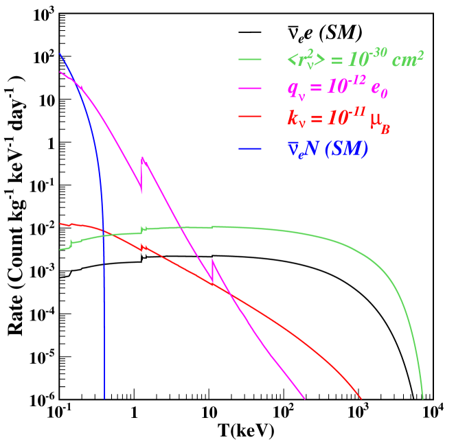
Figure 7: Expected measurable spectra with Ge on the various neutrino electromagnetic effects from reactor neutrinos ($\bar{\nu}_{e}$) at a flux of $10^{13}\,\mathrm{cm}^{-2}\,\mathrm{s}^{-1}$. The spectra from SM weak processes involving the electrons ($\bar{\nu}_{e}e$) and the nucleus ($\bar{\nu}_{e}N$) are also included for comparisons.

Data Set	Reactor-$\bar{\nu}_{e}$	Data Strength	Analysis	Bounds at 90% CL
	Flux	Reactor ON/OFF	Threshold	$\bbkappa_{\bar{\nu}_{e}}^{\mathrm{(eff)}}$	$\mathbbm{q}_{\bar{\nu}_{e}}$	$\langle\mathbbm{r}_{\bar{\nu}_{e}}^{2}\rangle^{\mathrm{(eff)}}$
	(${\rm\times 10^{13}~{}cm^{-2}s^{-1}}$)	(kg-days)	(keV)	($\times 10^{-11}~{}\mu_{{\rm B}}$)	($\times 10^{-12}$)	($\times 10^{-30}~{}\mbox{$\mathrm{cm}$}^{2}$)
TEXONO 187 kg CsI Deniz et al. (2010)	0.64	29882.0/7369.0	3000	< 22.0	< 170	< 0.033
TEXONO 1 kg Ge Li et al. (2003); Wong et al. (2007)	0.64	570.7/127.8	12	< 7.4	< 8.8	< 1.40
GEMMA 1.5 kg Ge Beda et al. (2012, 2013)	2.7	1133.4/280.4	2.8	< 2.9	< 1.1	< 0.80
TEXONO Point-Contact Ge Chen et al. (2014b, a)	0.64	124.2/70.3	0.3	< 26.0	< 2.1	< 3.20
Projected Point-Contact Ge	2.7	800/200	0.1	< 1.7	< 0.06	< 0.74
Sensitivity at $1\%$ of SM	—	—	—	$\sim$0.023	$\sim$0.0004	$\sim$0.0014

Summary of experimental limits at 90% CL on the various neutrino electromagnetic parameters studied in this work using selected reactor neutrino data. The projected sensitivities of measurements at the specified realistically experimental parameters are also shown. The last row illustrates the effective lower bounds to the sensitivities when a 1% measurement of the SM cross-section could be achieved, at threshold of 0.1 keV for $\bbkappa_{\bar{\nu}_{e}}^{\mathrm{(eff)}}$and $\mathbbm{q}_{\bar{\nu}_{e}}$, and 3 MeV for $\langle\mathbbm{r}_{\bar{\nu}_{e}}^{2}\rangle^{\mathrm{(eff)}}$, respectively.

IV.3 Neutrinos of Tritium $\beta$ Decay

The possibility of using the very low energy $\beta$ neutrinos from tritium decay to constrain neutrino magnetic moments was discussed in Refs. Kopeikin et al. (2003); Giomataris and Vergados (2004); McLaughlin and Volpe (2004). In Fig. 8, we compare the convoluted differential cross sections calculated by our MCRRPA approach, Ref. Kopeikin et al. (2003), and the FEA scheme.

As shown by the figure, below $T<1\,\mathrm{keV}$, FEA predicts larger cross sections for both neutrino weak and magnetic moment scattering than the two realistic many-body calculations. This echoes our previous argument that the Voloshin sum rule and FEA only poses an upper limit on cross sections, and the binding of an electron is not the only factor that determines whether FEA can be a good approximation or not. For $T>0.9\,\mathrm{keV}$ and $T>0.5\,\mathrm{keV}$, FEA predictions drop quickly below the realistic calculations for weak and magnetic moment scattering, respectively. This is mainly because the maximum energy transfer allowed by FEA: $T_{\max}=1.2\,\mathrm{keV}$ ($Q$ value for tritium $\beta$ decay is 18.6 keV) heavily restricts the allowed final-state phase space for scattering.

While our MCRRPA approach agrees with the previous many-body calculations Kopeikin et al. (2003) in the $T>0.9\,\mathrm{keV}$ and $T>0.5\,\mathrm{keV}$ regions for weak and magnetic moment scattering, respectively; our results are comparatively smaller at lower $T$. This discrepancy is mostly related to the treatments in atomic many-body physics: (i) Ref. Kopeikin et al. (2003) adopted the same framework as Refs. Fayans et al. (1992); Kopeikin et al. (1997); Fayans et al. (2001) by using the relativistic Dirac-Hartree-Fock method with a local exchange potential to solve the atomic ground-state structure, while we used he exact non-local Fock potential. (ii) The local exchange potential used by Ref. Kopeikin et al. (2003) is adapted from Ref.Moruzzi et al. (1978). This local exchange potential is designed to describe the ground-state structure of several metals (with Z<50) in the framework of density functional theory (DFT), therefore, it is not a surprise that it fits better the $M$-shell single particle energies of germanium crystal than our atomic calculations, because solid effects have been accounted for to some extent. (iii) It is known to be challenging to extend DFT to excited states (such as the ionization states which are relevant here); it is not clear how well the simplified mean-field scheme used by Ref. Kopeikin et al. (2003) can reproduce the photoabsorption data, say for $T>100\,\mathrm{eV}$—which we take as a very important benchmark for the computation of transition matrix elements.

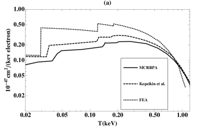
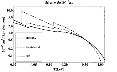
Figure 8: Differential cross sections of germanium ionization by neutrinos of tritium $\beta$ decay through (a) weak and (b) neutrino magnetic moment interaction assuming $\bbkappa_{\nu}^{\mathrm{(eff)}}=5\times 10^{-12}\mu_{\mathrm{B}}$.

V Summary and Prospects

In this paper, we show that the multiconfiguration relativistic random phase approximation provides a good description for the structure of germanium atoms and the photoabsorption data of germanium solid at photon energy $\gtrsim 80\,\mathrm{eV}$. These benchmark calculations justify a good understanding of how germanium detectors respond to neutrinos, through weak and possible electromagnetic interactions, with a threshold as low as $100\,\mathrm{eV}$.

After taking atomic ionization effects into account, existing reactor neutrino data with germanium detectors Beda et al. (2012, 2013) provide the most stringent direct experimental limits on neutrino millicharge and magnetic moments: $1.1\times 10^{-12}\,e$ and $2.9\times 10^{-11}\,\mu_{\mathrm{B}}$ at 90% confidence level, respectively. Future experiments with 100 eV threshold can target at the $10^{-14}\,e$ and $10^{-12}\,\mu_{\mathrm{B}}$ sensitivity range. In particular, there is substantial enhancement of the millicharge-induced cross section at low energy, providing smoking-gun signatures for positive signals. Charge-radius-induced interactions, on the other hand, do not have enhancement at low energy, such that the best sensitivities are obtained in experiment Deniz et al. (2010) with larger detector mass operating at the MeV energy range where the signal-to-background ratio is much more favorable.

The approach explored in this article as well as adopted by current laboratory experiments and astrophysics studies rely on searching possible anomalous effects relative to those produced by SM electroweak processes. It would therefore be experimentally difficult to probe non-standard effects less than, for example, 1% that of SM. There are certain fundamental (limited by physics rather than technology) lower bounds where such laboratory limits and astrophysics constraints can reach, as illustrated in Table IV.2. This limitation can be evaded, at least conceptually, by the analog of "appearance" experiments with the studies of detector channels where the SM background vanishes. For instance, in the case of Majorana neutrinos with transition magnetic moments, one can look for signatures of final-state neutrinos with a different flavor in a pure and intense neutrino beam which passes through a dense medium or an intense magnetic field. While there is no fundamental constraint to the lower reach of the sensitivities, realistic experiments are still many order-of-magnitude less sensitive than the reactor neutrino bounds Gonzalez-Garcia et al. (1996); Frère et al. (1997).

Appendix A Multipole Expansion

First we set up the coordinate system so that the 3-momentum transfer by neutrinos is along the $z$-axis, i.e., the Cartesian unit vector $\hat{e}_{3}=\vec{q}/|\vec{q}|$. The transformation between the unit vectors in the spherical ($\hat{\epsilon}^{\lambda=\pm 1,0}$) and Cartesian ($\hat{e}^{i=1,2,3}$) systems is then given by

$$\hat{\epsilon}^{\pm 1}=\mp\frac{1}{\sqrt{2}}(\hat{e}^{1}\pm i\hat{e}^{2})\,,\qquad\hat{\epsilon}^{0}=\hat{e}^{3}\,.$$ (48)

The spherical component of a vector $\vec{V}$, denoted by $\lambda$,  is

$$V^{\lambda}=\hat{\epsilon}^{\lambda}\cdot\vec{V}\,.$$ (49)

According to Eq. (43), the perturbing field that gives rise to atomic ionization by neutrino electromagnetic interactions takes the form

$$\left<\Psi_{f}\left|v_{+}^{(\gamma)}\right|\Psi_{i}\right> =\frac{4\pi\alpha}{q^{2}}\left\{j_{0}^{(\gamma)}\left\langle\Psi_{f}\left|\int d^{3}x\,e^{i\vec{q}\cdot\vec{x}}\hat{\mathcal{J}^{0}}(\vec{x})\right|\Psi_{i}\right\rangle\right.$$

$$\left.+\sum_{\lambda=\pm 1,0}(-1)^{\lambda}j_{\lambda}^{(\gamma)}\left\langle\Psi_{f}\left|\int d^{3}x\,e^{i\vec{q}\cdot\vec{x}}\hat{\epsilon}^{-\lambda}\cdot\hat{\vec{\mathcal{J}}}(\vec{x})\right|\Psi_{i}\right\rangle\right\}\,.$$ (50)

Using the relations

$$e^{i\vec{q}\cdot\vec{x}} =\sum_{J=0}^{\infty}\sqrt{4\pi(2J+1)}i^{J}j_{J}(\kappa r)Y_{J}^{0}(\Omega_{x})\,,$$ (51)

$$e^{i\vec{q}\cdot\vec{x}}\hat{\epsilon}^{0} =\frac{-i}{\kappa}\sum_{J=0}^{\infty}\sqrt{4\pi(2J+1)}i^{J}\overrightarrow{\nabla}\left[j_{J}(\kappa r)Y_{J}^{0}(\Omega_{x})\right]\,,$$ (52)

$$e^{i\vec{q}\cdot\vec{x}}\hat{\epsilon}^{\pm 1} =-\sum_{J\geq 1}\sqrt{2\pi(2J+1)}i^{J}\left\{\frac{1}{\kappa}\overrightarrow{\nabla}\times\left[j_{J}(\kappa r)\mathcal{Y}_{JJ1}^{\pm 1}(\Omega_{x})\right]\pm j_{J}(\kappa r)\mathcal{Y}_{JJ1}^{\pm 1}(\Omega_{x})\right\}\,,$$ (53)

where $|\vec{q}|\equiv\kappa$, $|\vec{x}|\equiv r$, $j_{J}(\kappa r)$ is the spherical Bessel function of order $J$, $Y_{J}^{M}(\Omega_{x})$ the spherical harmonics, and $\mathcal{Y}_{Jl1}^{M}(\Omega_{x})$ the vector spherical harmonics formed by adding $Y_{l}^{m}(\Omega_{x})$ and $\hat{\epsilon}^{\lambda}$ to be an angular momentum eigenstate $\ket{JM}$:

$$\mathcal{Y}_{Jl1}^{M}(\Omega_{x})\equiv\sum_{m\lambda}\left\langle lm1\lambda|l1JM\right\rangle Y_{l}^{m}(\Omega_{x})\hat{\epsilon}^{\lambda}\,,$$ (54)

the perturbing field is expanded as

$$\left<\Psi_{f}\left|v_{+}^{(\gamma)}\right|\Psi_{i}\right> =\frac{4\pi\alpha}{q^{2}}\left\{\sum_{J=0}^{\infty}\sqrt{4\pi(2J+1)}i^{J}\left[j_{0}^{(\gamma)}\braket{\hat{C}_{J0}(\kappa)}-j_{3}^{(\gamma)}\braket{\hat{L}_{J0}(\kappa)}\right]\right.$$

$$\left.+\sum_{J\geq 1}^{\infty}\sqrt{2\pi(2J+1)}i^{J}\sum_{\lambda=\pm 1}j_{\lambda}^{(\gamma)}\left[\braket{\hat{E}_{J-\lambda}(\kappa)}-\lambda\braket{\hat{M}_{J-\lambda}(\kappa)}\right]\right\}\,.$$ (55)

The various spherical multipole operators are defined by

$$\hat{C}_{JM}(\kappa) = \int d^{3}x\,[j_{J}(kr)Y_{JM}]\,\hat{\mathcal{J}}^{0}(\vec{x})\,,$$ (56)

$$\hat{L}_{JM}(\kappa) = \frac{i}{\kappa}\int d^{3}x\,\overrightarrow{\nabla}[j_{J}(\kappa r)Y_{JM}(\Omega_{x})]\cdot\hat{\vec{\mathcal{J}}}(\vec{x})$$ (57)

$$\hat{E}_{JM}(k) = \frac{1}{\kappa}\int d^{3}x\,\overrightarrow{\nabla}\times[j_{J}(\kappa r)\mathcal{Y}_{JJ1}^{M}(\Omega_{x})]\cdot\hat{\vec{\mathcal{J}}}(\vec{x})$$ (58)

$$\hat{M}_{JM}(k) = \int d^{3}x\,[j_{J}(\kappa r)\mathcal{Y}_{JJ1}^{M}(\Omega_{x})]\cdot\hat{\vec{\mathcal{J}}}(\vec{x})\,.$$ (59)

Each operator has its specific angular momentum and parity selections rules that restrict the possible initial-to-final-state transitions.

When dealing with weak interactions, the axial vector current operator $\hat{\mathcal{J}}_{5}(\vec{x})$ generates additional four types of multipole operators $\hat{C}_{JM}^{5}$, $\hat{L}_{JM}^{5}$, $\hat{E}_{JM}^{5}$, and $\hat{M}_{JM}^{5}$. They are obtained simply by replacing the vector current operator $\hat{\mathcal{J}}(\vec{x})$ with $\hat{\mathcal{J}}_{5}(\vec{x})$ in the above definitions.

References

- Giunti and Studenikin (2014) C. Giunti and A. Studenikin, (2014), arXiv:1403.6344 [hep-ph] .
- Broggini et al. (2012) C. Broggini, C. Giunti, and A. Studenikin, Adv. High Energy Phys. 2012, 459526 (2012).
- Wong and Li (2005) H. T. Wong and H. B. Li, Mod. Phys. Lett. A 20, 1103 (2005).
- Olive et al. (2014) K. Olive et al. (Particle Data Group), Chin. Phys. C 38, 090001 (2014).
- Wong et al. (2010) H. T. Wong, H.-B. Li, and S.-T. Lin, Phys. Rev. Lett. 105, 061801 (2010), erratum: arXiv:1001.2074v3.
- Chen et al. (2014a) J.-W. Chen, H.-C. Chi, H.-B. Li, C.-P. Liu, L. Singh, et al., (2014a), arXiv:1405.7168 [hep-ph] .
- Li et al. (2003) H. B. Li et al., Phys. Rev. Lett. 90, 131802 (2003).
- Wong et al. (2007) H. T. Wong et al., Phys. Rev. D 75, 012001 (2007).
- Beda et al. (2012) A. Beda et al., Adv. High Energy Phys. 2012, 350150 (2012).
- Beda et al. (2013) A. G. Beda et al., Phys. Part. Nucl. Lett. 10, 139 (2013).
- Deniz et al. (2010) M. Deniz et al. (TEXONO Collaboration), Phys. Rev. D 82, 033004 (2010), arXiv:1006.1947 [hep-ph] .
- Gninenko et al. (2007) S. Gninenko, N. Krasnikov, and A. Rubbia, Phys. Rev. D 75, 075014 (2007), arXiv:hep-ph/0612203 [hep-ph] .
- Studenikin (2013) A. Studenikin, (2013), arXiv:1302.1168 [hep-ph] .
- Lin et al. (2009) S. T. Lin et al., Phys. Rev. D 79, 061101 (2009).
- Li et al. (2013) H. B. Li et al., Phys. Rev. Lett. 110, 261301 (2013).
- Zhao et al. (2013) W. Zhao et al., Phys. Rev. D 88, 052004 (2013).
- Agnese et al. (2014) R. Agnese et al. (SuperCDMS Collaboration), Phys. Rev. Lett. 112, 241302 (2014), arXiv:1402.7137 [hep-ex] .
- Kouzakov and Studenikin (2014) K. A. Kouzakov and A. I. Studenikin, (2014), arXiv:1406.4999 [hep-ph] .
- Chen et al. (2014b) J.-W. Chen, H.-C. Chi, K.-N. Huang, C.-P. Liu, H.-T. Shiao, et al., Phys. Lett. B 731, 159 (2014b), arXiv:1311.5294 [hep-ph] .
- Fayans et al. (1992) S. Fayans, V. Y. Dobretsov, and A. Dobrotsvetov, Phys. Lett. B 291, 1 (1992).
- Kopeikin et al. (1997) V. I. Kopeikin, L. A. Mikaelyan, V. V. Sinev, and S. A. Fayans, Phys. At. Nucl. 60, 1859 (1997).
- Fayans et al. (2001) S. Fayans, L. Mikaelyan, and V. Sinev, Phys. Atom. Nucl. 64, 1475 (2001).
- Kopeikin et al. (2003) V. Kopeikin, L. Mikaelian, and V. Sinev, Phys. Atom. Nucl. 66, 707 (2003).
- Voloshin (2010) M. B. Voloshin, Phys. Rev. Lett. 105, 201801 (2010), erratum: ibid. 106, 059901 (2011).
- Kouzakov and Studenikin (2011) K. A. Kouzakov and A. I. Studenikin, Phys. Lett. B 696, 252 (2011).
- Kouzakov et al. (2011) K. A. Kouzakov, A. I. Studenikin, and M. B. Voloshin, Phys. Rev. D 83, 113001 (2011).
- Giomataris and Vergados (2004) Y. Giomataris and J. D. Vergados, Nucl. Instrum. Meth. A 530, 330 (2004).
- McLaughlin and Volpe (2004) G. C. McLaughlin and C. Volpe, Phys. Lett. B 591, 229 (2004).
- Musolf and Holstein (1991) M. J. Musolf and B. R. Holstein, Phys. Rev. D 43, 2956 (1991).
- von Weizsacker (1934) C. F. von Weizsacker, Z. Phys. 88, 612 (1934).
- Williams (1934) E. J. Williams, Phys. Rev. 45, 729 (1934).
- Greiner and Reinhardt (2009) W. Greiner and J. Reinhardt, Quantum Electrodynamics, 4th ed. (Springer, 2009).
- Chen et al. (2013) J.-W. Chen, C.-P. Liu, C.-F. Liu, and C.-L. Wu, Phys. Rev. D 88, 033006 (2013).
- Huang et al. (1995) K.-N. Huang, H.-C. Chi, and H.-S. Chou, Chin. J. Phys. 33, 565 (1995).
- Huang and Johnson (1982) K.-N. Huang and W. R. Johnson, Phys. Rev. A 25, 634 (1982).
- Huang (1982) K.-N. Huang, Phys. Rev. A 26, 734 (1982).
- Johnson and Huang (1982) W. R. Johnson and K.-N. Huang, Phys. Rev. Lett. 48, 315 (1982).
- Desclaux (1975) J. P. Desclaux, Comp. Phys. Comm. 9, 31 (1975).
- Henke et al. (1993) B. L. Henke, E. M. Gullikson, and J. C. Davis, At. Data Nucl. Data Tables 54, 181 (1993).
- Moruzzi et al. (1978) V. L. Moruzzi, J. F. Janak, and A. R. Williams, Calculated Electronic Properties of Metals (Pergamon, Oxford, 1978).
- Gonzalez-Garcia et al. (1996) M. Gonzalez-Garcia, F. Vannucci, and J. Castromonte, Phys. Lett. B 373, 153 (1996), arXiv:hep-ph/9510316 [hep-ph] .
- Frère et al. (1997) J. Frère, R. Nevzorov, and M. Vysotsky, Phys. Lett. B 394, 127 (1997), arXiv:hep-ph/9608266 [hep-ph] .