Incorporating Views on Marginal Distributions in the Calibration of Risk Models

Abstract

Entropy based ideas find wide-ranging applications in finance for calibrating models of portfolio risk as well as options pricing. The abstracted problem, extensively studied in the literature, corresponds to finding a probability measure that minimizes relative entropy with respect to a specified measure while satisfying constraints on moments of associated random variables. These moments may correspond to views held by experts in the portfolio risk setting and to market prices of liquid options for options pricing models. However, it is reasonable that in the former settings, the experts may have views on tails of risks of some securities. Similarly, in options pricing, significant literature focuses on arriving at the implied risk neutral density of benchmark instruments through observed market prices. With the intent of calibrating models to these more general stipulations, we develop a unified entropy based methodology to allow constraints on both moments as well as marginal distributions of functions of underlying securities. This is applied to Markowitz portfolio framework, where a view that a particular portfolio incurs heavy tailed losses is shown to lead to fatter and more reasonable tails for losses of component securities. We also use this methodology to price non-traded options using market information such as observed option prices and implied risk neutral densities of benchmark instruments.

1 Introduction

Entropy based ideas have found a number of popular applications in finance over the last two decades. A key application involves portfolio optimization where we often have a prior probability model and some independent expert views on the assets involved. If such views are of the form of constraints on moments, entropy based methods are used (see, e.g., Meucci [16]) to arrive at a ‘posterior’ probability measure that is closest in the sense of minimizing relative entropy or $I$-divergence to the prior probability model while satisfying those moment constraints. Another important application involves calibrating the risk neutral probability measure used for pricing options (see, e.g., Buchen and Kelly [6], Stutzer [20], Avellaneda et al. [2]). Here, entropy based ideas are used to arrive at a probability measure that correctly prices given liquid options (which are expectations of option payoffs) while again being closest to a specified prior probability measure.

As indicated, in the existing literature the conditions imposed on the posterior measure correspond to constraints on the moments of the underlying random variables. However, the constraints that arise in practice may be more general. For instance, in portfolio optimization settings, an expert may have a view that a certain index of stocks has a fat-tailed t-distribution, and is looking for a posterior joint distribution as a model of stock returns that satisfies this requirement while being closest to a prior model, that may, for instance, be based on historical data.

Similarly, a view on the risk neutral density of a certain financial instrument would also be reasonable if it is heavily traded, e.g., futures contract on a market index, and such views on marginal densities can be used to better price less liquid instruments that are correlated with the heavily traded instrument. There is now a sizable literature that focuses on estimating the implied risk neutral density from the observed option prices of an asset that has a highly liquid options market (see [14] for a comprehensive review). In [12], Figlewski notes that the implied risk neutral density of the US market portfolio, as a whole entity, implicitly captures market’s expectations, investors’ risk preferences and sensitivity to information releases and events. This is usually not possible with just a finite number of constraints on expected values of payoffs from options. So in the options pricing scenario, views on the posterior measure could include, for example, those on the the implied risk neutral density of a security price estimated from certain heavily traded options written on that security. See, for example, Avellaneda [1] for a discussion on the need to use all the available econometric information and stylized market facts to accurately calibrate mathematical models.

Motivated by these considerations, in this paper we devise a methodology to arrive at a posterior probability measure when the constraints on this measure are of a general nature that, apart from moment constraints, include specifications of marginal distributions of functions of underlying random variables as well.

Related literature: The evolving literature on updating models for portfolio optimization to include specified views builds upon the pioneering work of Black and Litterman [4]. They consider variants of Markowitz’s model where the subjective views of portfolio managers are used as constraints to update models of the market using ideas from Bayesian analysis. Their work focuses on Gaussian framework with views restricted to linear combinations of expectations of returns from different securities. Since then a number of variations and improvements have been suggested (see, e.g., [17], [18] and [19]). Earlier, Avellaneda et al. [2] used weighted Monte Carlo methodology to calibrate asset pricing models to market data (also see Glasserman and Yu [13]). Buchen and Kelly in [6] and Stutzer in [20] use the entropy approach to calibrate one-period asset pricing models by selecting a pricing measure that correctly prices a set of benchmark instruments while minimizing $I$-divergence from a prior specified model, that may, for instance be estimated from historical data (see the recent survey article [15]).

Our contributions: As mentioned earlier, we focus on examples related to portfolio optimization and options pricing. It is well known that for views expressed as a finite number of moment constraints, the optimal solution to the $I$-divergence minimization can be characterized as a probability measure obtained by suitably exponentially twisting the original measure; this exponentially twisted measure is known in literature as the Gibbs measure (see, for instance, [9]). We generalize this to allow cases where the expert views may specify marginal probability distribution of functions of random variables involved. We show that such views, in addition to views on moments of functions of underlying random variables can be easily incorporated. In particular, under technical conditions, we characterize the optimal solution with these general constraints, when the objective is $I$-divergence and show the uniqueness of the resulting optimal probability measure.

As an illustration, we apply our results to portfolio modeling in Markowitz framework where the returns from a finite number of assets have a multivariate Gaussian distribution and expert view is that a certain portfolio of returns is fat-tailed. We show that in the resulting probability measure, under mild conditions, all correlated assets are similarly fat-tailed. Hence, this becomes a reasonable way to incorporate realistic tail behavior in a portfolio of assets. Generally speaking, the proposed approach may be useful in better risk management by building conservative tail views in mathematical models. We also apply our results to price an option which is less liquid and written on a security that is correlated with another heavily traded asset whose risk neutral density is inferred from the options market prices. We conduct numerical experiments on practical examples that validate the proposed methodology.

Organization of the paper: We formulate the model selection problem as an optimization problem in Section 2, and derive the posterior probability model as its solution in Section 3. In Section 4, we apply our results to the portfolio problem in the Markowitz framework and develop explicit expressions for the posterior probability measure. There we also show how a view that a portfolio of assets has a ‘regularly varying’ fat-tailed distribution renders a similar fat-tailed marginal distribution to all assets correlated to this portfolio. Further, we numerically test our proposed algorithms on practical examples. In Section 5, we illustrate the applicability of the proposed framework in options pricing scenario. Finally, we end in Section 6 with a brief conclusion. All but the simplest proofs are relegated to the Appendix.

2 The Model Selection Problem

In this section, we briefly review the notion of relative entropy between probability measures and use it to formally state our model selection problem.

2.1 Relative Entropy and its Variational Representation

Let $(\Omega,\mathcal{F})$ denote a measurable space and $\mathcal{P}$ denote the set of all probability measures on $(\Omega,\mathcal{F}).$ If a measure $\nu$ on $(\Omega,\mathcal{F})$ is absolutely continuous with respect to $\mu,$ we denote this by $\nu\ll\mu.$ For any $\nu,\mu\in\mathcal{P},$ the relative entropy of $\nu$ with respect to $\mu$ (also known as $I$-divergence or Kullback-Leibler divergence) is defined as

$$D(\nu||\mu):=\begin{cases}\int\log\left(\frac{{\mathnormal{d}}\nu}{{\mathnormal{d}}\mu}\right){\mathnormal{d}}\nu,&\text{ if }\nu\ll\mu,\\ \infty,&\text{ otherwise.}\end{cases}$$

For any bounded measurable function $\psi$ mapping $\Omega$ into $\mathbb{R},$ it is well known that,

$$\log\int_{\Omega}e^{\psi}d\mu=\sup_{\nu}\left\{\int_{\Omega}\psi\,d\nu-D(\nu\mid\mid\mu)\right\}.$$ (1)

Furthermore, this supremum is attained at $\nu^{*}$ given by:

$$\frac{d\nu^{*}}{d\mu}=\frac{e^{\psi}}{\int e^{\psi}\,d\mu}.$$ (2)

See, for instance, [10] for a proof of this and for other concepts related to relative entropy.

2.2 Problem Formulation

Let the random vectors ${\bf X}=(X_{1},\ldots,X_{m})$ and ${\bf Y}=(Y_{1},\ldots,Y_{n})$ denote the risk factors associated with the prior reference risk model, which is specified as a joint probability density $f({\bf x,y})$ over ${\bf X}$ and ${\bf Y}.$ This model, typically arrived using statistical analysis of historical data, is used for risk analysis (such as calculating expected shortfall, VaR, etc.), or for choosing optimal positions in portfolios. However, the market presents itself with additional information, usually in the form of ‘views’ of experts (or) current market observables. These views can be simple moment constraints as in,

$$\int_{\bf x,y}h_{i}({\bf x,y})\mathbb{P}({\mathnormal{d}}{\bf x},{\mathnormal{d}}{\bf y})=c_{i},i=1,\ldots,k,$$

(or) as detailed as constraints over marginal densities:

$$\int_{\bf y}\mathbb{P}({\mathnormal{d}}{\bf x},{\mathnormal{d}}{\bf y})=g({\bf x})\text{ for all {\bf x}},$$

where $c_{i},i=1,\ldots,k$ are constants, $g(\cdot)$ is a given marginal density of ${\bf X}$ and $\mathbb{P}(\cdot)$ is the unknown probability measure governing the risk factors. Then our objective is to identify a probability model that has minimum relative entropy with respect to the prior model $f(\cdot,\cdot)$ while agreeing with the views on moments of ${\bf Y}$ and marginal distribution of ${\bf X}.$ Though relative entropy $D(\cdot||\cdot)$ is not a metric, it has been widely used to discriminate between probability measures in the context of model calibration (see [7], [6], [20],[3], [1], [2], [16] and [15]). Let $\mathcal{P}(f)$ denote the collection of probability density functions which are absolutely continuous with respect to the density $f(\cdot,\cdot)$ (a density $\tilde{f}(\cdot,\cdot)$ is said to be absolutely continuous with respect to $f(\cdot,\cdot)$ if for almost every $x$ and $y$ such that $f(x,y)=0,$ $\tilde{f}(x,y)$ also equals $0$). Formally, the resulting optimization problem ${\bf O_{1}}$ is:

$$\min_{\tilde{f}\in\mathcal{P}(f)}\int\log\left(\frac{\tilde{f}(\mathbb{x},\mathbb{y})}{f(\mathbb{x},\mathbb{y})}\right)\tilde{f}(\mathbb{x},\mathbb{y})d\mathbb{x}d\mathbb{y},$$

subject to:

$$\int_{\mathbb{y}}\tilde{f}(\mathbb{x},\mathbb{y})d\mathbb{y}=g(\mathbb{x})\,\,\,\text{for all}\,\,\,\mathbb{x},\text{ and }$$ (3a)

$$\int_{\mathbb{x},\mathbb{y}}h_{i}(\mathbb{x},\mathbb{y})\tilde{f}(\mathbb{x},\mathbb{y})d\mathbb{x}d\mathbb{y}=c_{i},i=1,2\ldots,k.$$ (3b)

3 Solution to the Optimization Problem ${\bf O_{1}}$

Some notation is needed to proceed further. For any $\mbox{\boldmath{$\lambda$}}=(\lambda_{1},\lambda_{2},\ldots,\lambda_{k})\in\mathbb{R}^{k},$ let

$$f_{\mbox{\boldmath{$\lambda$}}}(\mathbb{y}|\mathbb{x}):=\frac{\exp(\sum_{i=1}^{k}\lambda_{i}h_{i}(\mathbb{x},\mathbb{y})){f}(\mathbb{y}|\mathbb{x})}{\int_{\mathbb{y}}\exp(\sum_{i=1}^{k}\lambda_{i}h_{i}(\mathbb{x},\mathbb{y})){f}(\mathbb{y}|\mathbb{x}){\mathnormal{d}}\mathbb{y}}=\frac{\exp(\sum_{i=1}^{k}\lambda_{i}h_{i}(\mathbb{x},\mathbb{y})){f}(\mathbb{x},\mathbb{y})}{\int_{\mathbb{y}}\exp(\sum_{i=1}^{k}\lambda_{i}h_{i}(\mathbb{x},\mathbb{y})){f}(\mathbb{x},\mathbb{y}){\mathnormal{d}}\mathbb{y}}$$

whenever the denominator exists. Further, let $f_{\mbox{\boldmath{$\lambda$}}}(\mathbb{x},\mathbb{y}):=f_{\mbox{\boldmath{$\lambda$}}}(\mathbb{y}|\mathbb{x})\times g(\mathbb{x})$ denote a joint density function of $(\mathbb{X},\mathbb{Y})$ and $\mathbb{E}_{\mbox{\boldmath{$\lambda$}}}[\cdot]$ denote the expectation under $f_{\mbox{\boldmath{$\lambda$}}}(\cdot,\cdot)$. Let $m_{g}(\cdot)$ be the measure corresponding to the probability density $g(\cdot)$ on $\mathbb{R}^{m}.$ For a mathematical claim that depends on ${\bf x}\in\mathbb{R}^{m},$ say $S({\bf x}),$ we write $S({\bf x})$ for almost all ${\bf x},$ with respect to $g({\bf x}){\mathnormal{d}}{\bf x}$ to mean that $m_{g}(\{{\bf x}:S({\bf x})\text{is false}\})=0.$

Theorem 1.

If there exists a $\mbox{\boldmath{$\lambda$}}=(\lambda_{1},\ldots,\lambda_{k})\in\mathbb{R}^{k}$ such that

1. $\int_{\mathbb{y}}\exp(\sum_{i}\lambda_{i}h_{i}({\bf x,y})){f}(\mathbb{x},\mathbb{y})d\mathbb{y}<\infty$ for almost all $\mathbb{x}$ with respect to $g(\mathbb{x})d\mathbb{x}$, and

2. $E_{\mbox{\boldmath{$\lambda$}}}[h_{i}(\mathbb{X},\mathbb{Y})]=c_{i},$ for $i=1,\ldots,k,$

then $f_{\mbox{\boldmath{$\lambda$}}}(\cdot)$ is an optimal solution to the optimization problem ${\bf O_{1}}$.

It is natural to ask for conditions under which such a $\mbox{\boldmath{$\lambda$}}=(\lambda_{1},\ldots,\lambda_{k})$ exists. Here, we provide a simple condition in Remark 1 below. A further set of elaborate conditions can be found in Theorem 3.1 of [8].

Remark 1 (On the existence of $\lambda$).

For every $(c_{1},\ldots,c_{k})$ in the interior of convex hull of the support of the probability density function induced on $\mathbb{R}^{k}$ by the mapping $({\bf x},{\bf y})\longmapsto(h_{1}({\bf x},{\bf y}),\ldots,h_{k}({\bf x},{\bf y})),$ it follows from Theorem 3.1 of [8] that there exists a $(\lambda_{1},\ldots,\lambda_{k})$ satisfying conditions of Theorem 1.

Proof of Theorem 1.

In view of (3a), we may fix the marginal distribution of $\mathbb{X}$ to be $g(\mathbb{x})$ and re-express the objective as

$$\min_{\tilde{f}(\cdot|\mathbb{x})\in{\cal P}({f}(\cdot|\mathbb{x})),\forall\mathbb{x}}\int_{\mathbb{x},\mathbb{y}}\log\left(\frac{\tilde{f}(\mathbb{y}|\mathbb{x})}{f(\mathbb{y}|\mathbb{x})}\right)\tilde{f}(\mathbb{y}|\mathbb{x})g(\mathbb{x})d\mathbb{y}d\mathbb{x}+\int_{\mathbb{x}}\log\left(\frac{g(\mathbb{x})}{f(\mathbb{x})}\right)g(\mathbb{x})d\mathbb{x}\,.$$

The second integral is a constant and can be dropped from the objective. The first integral can be expressed as

$$\int_{\mathbb{x}}\min_{\tilde{f}(\cdot|\mathbb{x})\in{\cal P}({f}(\cdot|\mathbb{x}))}\left(\int_{\mathbb{y}}\log\frac{\tilde{f}(\mathbb{y}|\mathbb{x})}{f(\mathbb{y}|\mathbb{x})}\tilde{f}(\mathbb{y}|\mathbb{x})d\mathbb{y}\right)g(\mathbb{x})d\mathbb{x}\,.$$

Similarly the moment constraints can be re-expressed as

$$\int_{\mathbb{x},\mathbb{y}}h_{i}(\mathbb{x},\mathbb{y})\tilde{f}(\mathbb{y}|\mathbb{x})g(\mathbb{x})d\mathbb{x}d\mathbb{y}=c_{i},\,\,\,i=1,2,...,k.$$

This, in turn, is same as:

$$\int_{\mathbb{x}}\left(\int_{\mathbb{y}}h_{i}(\mathbb{x},\mathbb{y})\tilde{f}(\mathbb{y}|\mathbb{x})d\mathbb{y}\right)g(\mathbb{x})d\mathbb{x}=c_{i},\,\,\,i=1,2,...,k\,.$$

Then, the Lagrangian for this $k$ constraint problem is,

$$\int_{\mathbb{x}}\left[\min_{\tilde{f}(\cdot|\mathbb{x})\in{\cal P}({f}(\cdot|\mathbb{x}))}\int_{\mathbb{y}}\left(\log\frac{\tilde{f}(\mathbb{y}|\mathbb{x})}{f(\mathbb{y}|\mathbb{x})}\tilde{f}(\mathbb{y}|\mathbb{x})-\sum_{i=1}^{k}\delta_{i}h_{i}(\mathbb{x},\mathbb{y})\tilde{f}(\mathbb{y}|\mathbb{x})\right)d\mathbb{y}\right]g(\mathbb{x})d\mathbb{x}+\sum_{i=1}^{k}\delta_{i}c_{i},$$

for $\delta_{i}\in\mathbb{R}.$ Note that by (2),

$$\min_{\tilde{f}(\cdot|\mathbb{x})\in{\cal P}({f}(\cdot|\mathbb{x}))}\int_{\mathbb{y}}\left(\log\frac{\tilde{f}(\mathbb{y}|\mathbb{x})}{f(\mathbb{y}|\mathbb{x})}\tilde{f}(\mathbb{y}|\mathbb{x})-\sum_{i}\delta_{i}h_{i}(\mathbb{x},\mathbb{y})\tilde{f}(\mathbb{y}|\mathbb{x})\right)dy$$

has the solution

$$f_{\mbox{\boldmath{$\delta$}}}(\mathbb{y}|\mathbb{x})=\frac{\exp(\sum_{i}\delta_{i}h_{i}(\mathbb{x},\mathbb{y})){f}(\mathbb{y}|\mathbb{x})}{\int_{\mathbb{y}}\exp(\sum_{i}\delta_{i}h_{i}(\mathbb{x},\mathbb{y})){f}(\mathbb{y}|\mathbb{x})d\mathbb{y}}=\frac{\exp(\sum_{i}\delta_{i}h_{i}(\mathbb{x},\mathbb{y})){f}(\mathbb{x},\mathbb{y})}{\int_{\mathbb{y}}\exp(\sum_{i}\delta_{i}h_{i}(\mathbb{x},\mathbb{y})){f}(\mathbb{x},\mathbb{y})d\mathbb{y}},$$

where we write $\delta$ for $(\delta_{1},\delta_{2},\ldots,\delta_{k})$. Now taking $\mbox{\boldmath{$\delta$}}=\mbox{\boldmath{$\lambda$}}$, it follows from the Assumptions (a) and (b) in the statement of Theorem 1 that $f_{\mbox{\boldmath{$\lambda$}}}(\mathbb{x},\mathbb{y})=f_{\mbox{\boldmath{$\lambda$}}}(\mathbb{y}|\mathbb{x})g(\mathbb{x})$ is a solution to the optimization problem ${\bf O_{1}}\,.$ ∎

In Theorem 2, we give conditions that ensure uniqueness of a solution to the optimization problem ${\bf O_{1}}$ whenever it exists. The proof of Theorem 2 is presented in the Appendix.

Theorem 2.

Suppose that for almost all ${\mathbb{x}}$ w.r.t. $g(\mathbb{x})d\mathbb{x}$, conditional on $\mathbb{X}=\mathbb{x}$, the random variables $h_{1}(\mathbb{x},\mathbb{Y}),h_{2}(\mathbb{x},\mathbb{Y}),\ldots,h_{k}(\mathbb{x},\mathbb{Y})$ are linearly independent. Then, if a solution to the constraint equations

$$E_{\mbox{\boldmath{$\lambda$}}}[h_{i}(\mathbb{X},\mathbb{Y})]=c_{i},i=1,\ldots,k$$

exists, it is unique.

Remark 2.

Theorem 1, as stated, is applicable when the updated marginal distribution of a sub-vector $\mathbb{X}$ of the given random vector $(\mathbb{X},\mathbb{Y})$ is specified. More generally, constraints on marginal densities and moments of functions of the given random vector can also be incorporated by a routine change of variable technique. This is illustrated below:

Let $\mathbb{Z}=(Z_{1},Z_{2},\ldots,Z_{N})$ denote a random vector taking values in $S\subseteq\mathbb{R}^{N}$ and having a (prior) density function $f_{\mathbb{Z}}(\cdot).$ Suppose the constraints on ${\bf Z}$ are as follows:

1. $\left(v_{1}(\mathbb{Z}),v_{2}(\mathbb{Z}),\ldots,v_{k_{1}}(\mathbb{Z})\right)$ have a joint density function given by $g(\cdot)$.

2. The moments of $v_{k_{1}+1}(\mathbb{Z}),\ldots,v_{k_{2}}(\mathbb{Z})$ are, respectively, $c_{1},\ldots,c_{k_{2}-k_{1}}.$

where $0\leq k_{1}\leq k_{2}\leq N$ and $v_{1}(\cdot),\,v_{2}(\cdot),\,\ldots,\,v_{k_{2}}(\cdot)$ are some functions on $S$. If the total number of constraints $k_{2}$ is smaller than $N,$ we define $N-k_{2}$ additional functions $v_{k_{2}+1}(\cdot),\,v_{k_{2}+2}(\cdot),\,\ldots,\,v_{N}(\cdot)$ such that the function $v:S\rightarrow\mathbb{R}^{N}$ defined by $v(\mathbb{z})=\left(v_{1}(\mathbb{z}),v_{2}(\mathbb{z}),\ldots,v_{N}(\mathbb{z})\right)$ has a non-singular Jacobian almost everywhere. That is,

$$J(\mathbb{z}):=\text{det}\left(\left(\frac{\partial v_{i}}{\partial z_{j}}\right)_{i,j}\right)\neq 0\,\,\text{for almost all}\,\,\mathbb{z}\,\,\text{w.r.t.}\,f_{\mathbb{Z}}.$$

This happens if the function $v$ is locally invertible almost everywhere. Now to compute the posterior density that minimizes the relative entropy with respect to the prior density $f_{\bf Z}(\cdot)$ while satisfying constraints (i) and (ii), we let

$$X_{i}=v_{i}(\mathbb{Z})\text{ for }i\leq k_{1},\mathbb{X}=(X_{1},\ldots,X_{k_{1}}),\text{ and }$$

$$Y_{i}=v_{k_{1}+i}(\mathbb{Z})\text{ for }i\leq N-k_{1},\mathbb{Y}=(Y_{1},\ldots,Y_{N-k_{1}}).$$

If we use $f(\cdot,\cdot)$ to denote the prior density function corresponding to $(\mathbb{X},\mathbb{Y})$ and $w(\cdot)$ to denote the local inverse function of $v(\cdot),$ then by the change of variables formula for densities,

$$f(\mathbb{x},\mathbb{y})=f_{\mathbb{Z}}\left(w(\mathbb{x},\mathbb{y})\right)[J\left(w(\mathbb{x},\mathbb{y})\right)]^{-1}.$$

Further, the constraints (i) and (ii) translate in terms of $(\mathbb{X},\mathbb{Y})$ into:

1. $\mathbb{X}\,\,\text{have joint density given by}\,\,g(\cdot)$ and

2. For $i=1,\ldots,k_{2}-k_{1},$ the expected value of $Y_{i}$ is $c_{i}.$

Setting $k=k_{2}-k_{1}$, it follows from Theorem 1 that the optimal joint density function of $(\mathbb{X},\mathbb{Y})$ is:

$$f_{\mbox{\boldmath{$\lambda$}}}(\mathbb{x},\mathbb{y})=\frac{e^{\lambda_{1}y_{1}+\lambda_{2}y_{2}+\cdots+\lambda_{k}y_{k}}f(\mathbb{x},\mathbb{y})}{\int_{y}e^{\lambda_{1}y_{1}+\lambda_{2}y_{2}+\cdots+\lambda_{k}y_{k}}f(\mathbb{x},\mathbb{y})\,d\mathbb{y}}\times g(\mathbb{x})\,,$$

where $\mathbb{\lambda}_{k}$s are chosen such that $\mathbb{E}_{\mbox{\boldmath{$\lambda$}}}[Y_{i}]=c_{i},i=1,\ldots,k.$ Again by changing the variables, it follows that the optimal density of $\mathbb{Z}$ is given by:

$$\tilde{f}_{\mathbb{Z}}(\mathbb{z})=f_{\mbox{\boldmath{$\lambda$}}}(v_{1}(\mathbb{z}),v_{2}(\mathbb{z}),\ldots,v_{N}(\mathbb{z}))J(\mathbb{z})\,\,.\,\,$$

It can be easily seen that the case of Jacobian being identity matrix corresponds to no change of variables, and we recover the solution to the original optimization problem ${\bf O_{1}}.$

Remark 3.

Suppose that a portfolio performance measure of interest is an expectation of some random variable $r(\mathbb{X},\mathbb{Y})$ under the posterior measure $f_{\mbox{\boldmath{$\lambda$}}}({\bf x,y}).$ Few examples of this measure include expected portfolio return, portfolio variance, or the probability that the portfolio loss exceeds a threshold. For $\mbox{\boldmath{$\gamma$}}\in\mathbb{R}^{k},$ let

$$\Pi(\mbox{\boldmath{$\gamma$}})=\mathbb{E}_{\mbox{\boldmath{$\gamma$}}}[r(\mathbb{X},\mathbb{Y})].$$

Then computing the sensitivity $\partial\Pi(\mbox{\boldmath{$\lambda$}})/\partial c_{i}$ is of practical interest (recall that $c_{i}$ is specified in Equation (3b)). This follows through an easy extension of analysis in [1]. Note that

$$\frac{\partial\Pi(\mbox{\boldmath{$\lambda$}})}{\partial c_{i}}=\sum_{j}\left(\frac{\partial\Pi(\mbox{\boldmath{$\gamma$}})}{\partial\gamma_{j}}\right)_{\mbox{\boldmath{$\gamma$}}=\mbox{\boldmath{$\lambda$}}}\frac{\partial\lambda_{j}}{\partial c_{i}}.$$

Further we have $\mathbb{E}_{\mbox{\boldmath{$\lambda$}}}[h_{i}({\bf X,Y})]=c_{i}.$ Following the lines of proof in the Appendix of [6], it can be verified that

$$\frac{\partial\Pi(\mbox{\boldmath{$\gamma$}})}{\partial\gamma_{j}} =\mathbb{E}\left[\textnormal{Cov}_{\mbox{\boldmath{$\gamma$}}}(r(\mathbb{X},\mathbb{Y}),h_{j}(\mathbb{X},\mathbb{Y})|\mathbb{X})\right],\text{ and }$$

$$\frac{\partial c_{i}}{\partial\lambda_{j}} =\mathbb{E}\left[\textnormal{Cov}_{\mbox{\boldmath{$\lambda$}}}(h_{i}(\mathbb{X},\mathbb{Y}),h_{j}(\mathbb{X},\mathbb{Y})|\mathbb{X})\right],$$

where

$$\textnormal{Cov}_{\mbox{\boldmath{$\gamma$}}}(r(\mathbb{X},\mathbb{Y}),h_{j}(\mathbb{X},\mathbb{Y})|\mathbb{X})=\mathbb{E}_{\mbox{\boldmath{$\gamma$}}}[r(\mathbb{X},\mathbb{Y})h_{j}(\mathbb{X},\mathbb{Y})|\mathbb{X}]-\mathbb{E}_{\mbox{\boldmath{$\gamma$}}}[r(\mathbb{X},\mathbb{Y})|\mathbb{X})\mathbb{E}_{\mbox{\boldmath{$\gamma$}}}(h_{j}(\mathbb{X},\mathbb{Y})|\mathbb{X}].$$

Let $V_{ij}=\partial c_{i}/\partial\lambda_{j}$ and $V$ be the matrix with $V_{ij}$ as its entries. Let $U=V^{-1}.$ Then using Implicit Function Theorem on $\mathbb{E}_{\mbox{\boldmath{$\lambda$}}}[h_{i}({\bf X,Y})]=c_{i},$ we have that

$$\frac{\partial\lambda_{j}}{\partial c_{i}}=U_{ij},$$

where $U_{ij}$ is the $(i,j)^{th}$ entry of the matrix $U.$ In particular,

$$\frac{\partial\Pi(\mbox{\boldmath{$\lambda$}})}{\partial c_{i}}=\sum_{j}\mathbb{E}\left[\textnormal{Cov}_{\mbox{\boldmath{$\lambda$}}}(r(\mathbb{X},\mathbb{Y}),h_{j}(\mathbb{X},\mathbb{Y})|\mathbb{X})\right]U_{ij}.$$

Similarly, suppose that the density function $g(\cdot)$ depends on a parameter $\alpha,$ which we express as $g_{\alpha}(\cdot),$ then it follows that

$$\frac{\partial\Pi(\mbox{\boldmath{$\lambda$}})}{\partial\alpha}=\mathbb{E}_{\mbox{\boldmath{$\lambda$}}}\left[r(\mathbb{X},\mathbb{Y})\frac{\frac{\partial g_{\alpha}(\mathbb{X})}{\partial\alpha}}{g_{\alpha}(\mathbb{X})}\right].$$

4 Portfolio Modeling in Markowitz Framework

In this section we apply the methodology developed in Section 3 to the Markowitz framework: Namely to the setting where there are $N$ assets whose returns under the ‘prior distribution’ are multivariate Gaussian. Here, we explicitly identify the posterior distribution that incorporates views/constraints on marginal distribution of some random variables and moment constraints on other random variables. As mentioned in the introduction, an important application of our approach is that if for a particular portfolio of assets, say an index, it is established that the return distribution is fat-tailed (specifically, the pdf is a regularly varying function), say with the density function $g(\cdot)$, then by using that as a constraint, one can arrive at an updated posterior distribution for all the underlying assets. Furthermore, we show that if an underlying asset has a non-zero correlation with this portfolio under the prior distribution, then under the posterior distribution, this asset has a tail distribution similar to that given by $g(\cdot)$.

Let $(\mathbb{X},\mathbb{Y})=(X_{1},X_{2},\ldots,X_{N-k},Y_{1},Y_{2},\ldots,Y_{k})$ have a $N$ dimensional multivariate Gaussian distribution with mean $\mbox{\boldmath{$\mu$}}=(\mbox{\boldmath{$\mu$}}_{\mathbb{x}},\mbox{\boldmath{$\mu$}}_{\mathbb{y}})$ and the variance-covariance matrix

$$\mathbb{\Sigma}=\left(\begin{array}[]{cc}\mathbb{\Sigma}_{\mathbb{xx}}&\mathbb{\Sigma}_{\mathbb{xy}}\\ \mathbb{\Sigma}_{\mathbb{yx}}&\mathbb{\Sigma}_{\mathbb{yy}}\end{array}\right).$$

Let $g(\cdot)$ be a given probability density function on $\mathbb{R}^{N-k}$ with finite first moments along each component and $\mathbb{a}$ be a given vector in $\mathbb{R}^{k}$. Then we look for a posterior measure $\tilde{\mathbb{P}}(\cdot)$ that satisfies the view that

$${\bf X}\,\,\text{has probability density function}\,\,g(\cdot)\,\,\text{and}\,\,\tilde{\mathbb{E}}(\mathbb{Y})=\mathbb{a}.$$

As discussed in Remark 2 (see also Example 2 in Section 5), when the view is on marginal distributions of linear combinations of underlying assets, and/or on moments of linear functions of the underlying assets, the problem can be easily transformed to the above setting by a suitable change of variables.

To find a distribution of $(\mathbb{X},\mathbb{Y})$ which incorporates the above views, we solve the minimization problem ${\bf O_{2}}$:

$$\min_{\tilde{f}\in{\cal P}(f)}\int_{(\mathbb{x},\mathbb{y})\in\mathbb{R}^{N-k}\times\mathbb{R}^{k}}\log\left(\frac{\tilde{f}(\mathbb{x},\mathbb{y})}{f(\mathbb{x},\mathbb{y})}\right)\tilde{f}(\mathbb{x},\mathbb{y})\,d\mathbb{x}d\mathbb{y}$$

subject to the constraint:

$$\int_{\mathbb{y}\in\mathbb{R}^{k}}\tilde{f}(\mathbb{x},\mathbb{y})d\mathbb{y}=g(\mathbb{x})\,\,\,\,\text{ for all }\mathbb{x}$$

and

$$\int_{\mathbb{x}\in\mathbb{R}^{N-k}}\int_{\mathbb{y}\in\mathbb{R}^{k}}\mathbb{y}\tilde{f}(\mathbb{x},\mathbb{y})d\mathbb{y}d\mathbb{x}=\mathbb{a},$$ (4)

where $f(\mathbb{x},\mathbb{y})$ is the density of $N$-variate normal distribution denoted by $\mathcal{N}_{N}(\mbox{\boldmath{$\mu$}},\mathbb{\Sigma})$.

Proposition 1.

Under the assumption that $\Sigma_{\mathbb{xx}}$ is invertible, the optimal solution to ${\bf O_{2}}$ is given by

$$\tilde{f}(\mathbb{x},\mathbb{y})=\tilde{f}(\mathbb{y}|\mathbb{x})\times g(\mathbb{x})$$ (5)

where $\tilde{f}(\mathbb{y}|\mathbb{x})$ is the probability density function of

$$\mathcal{N}_{k}\left(\mathbb{a}+\mathbb{\Sigma}_{\mathbb{yx}}\mathbb{\Sigma}_{\mathbb{xx}}^{-1}(\mathbb{x}-\mathbb{E}_{g}[\mathbb{X}])\,,\,\mathbb{\Sigma}_{\mathbb{yy}}-\mathbb{\Sigma}_{\mathbb{yx}}\mathbb{\Sigma}_{\mathbb{xx}}^{-1}\mathbb{\Sigma}_{\mathbb{xy}}\right)$$

where $\mathbb{E}_{g}[\mathbb{X}]$ is the expectation of ${\bf X}$ under the density function $g(\cdot)$.

Tail behavior of the marginals of the posterior distribution: We now specialize to the case where $\mathbb{X}$ (also denoted by $X$) is a real valued random variable so that $N=k+1$, and Assumption 1 below is satisfied by pdf $g(\cdot).$ Specifically, $(X,\mathbb{Y})$ is distributed as $\mathcal{N}_{k+1}(\mbox{\boldmath{$\mu$}},\mathbb{\Sigma})$ with

$$\mbox{\boldmath{$\mu$}}^{T}=(\mu_{x},\mbox{\boldmath{$\mu$}}_{\mathbb{y}}^{T})\,\,\,\text{and}\,\,\,\mathbb{\Sigma}=\left(\begin{array}[]{cc}\sigma_{xx}&\mbox{\boldmath{$\sigma$}}_{x\mathbb{y}}^{T}\\ \mbox{\boldmath{$\sigma$}}_{x\mathbb{y}}&\mathbb{\Sigma}_{\mathbb{yy}}\end{array}\right)$$

where $\mbox{\boldmath{$\sigma$}}_{x\mathbb{y}}=(\sigma_{xy_{{}_{1}}},\sigma_{xy_{{}_{2}}},...,\sigma_{xy_{{}_{k}}})^{T}$ with $\sigma_{xy_{{}_{i}}}=\textnormal{Cov}(X,Y_{i}).$

Assumption 1.

The pdf $g(\cdot)$ is regularly varying: that is, there exists a constant $\alpha>1$ (we require $\alpha>1$ so that $g(\cdot)$ is integrable) such that

$$\lim_{t\rightarrow\infty}\frac{g(\eta t)}{g(t)}=\frac{1}{\eta^{\alpha}}$$

for all $\eta>0$ (see, for instance, [11]). In addition, for any $a\in\mathbb{R}$ and $b\in\mathbb{R}^{+},$

$$\frac{g(b(t-s-a))}{g(t)}\leq h(s)$$ (6)

for some non-negative function $h(\cdot)$ independent of $t$ (but possibly depending on $a$ and $b$) with the property that $\mathbb{E}h(Z)<\infty$ whenever $Z$ has a Gaussian distribution.

Remark 4.

Assumption 1 holds, for instance, when $g(\cdot)$ corresponds to $t$-distribution with $n$ degrees of freedom, that is,

$$g(s)=\frac{\Gamma(\frac{n+1}{2})}{\sqrt{n\pi}\Gamma(\frac{n}{2})}\left(1+\frac{s^{2}}{n}\right)^{-\left(\frac{n+1}{2}\right)}\,,$$

Clearly, $g(\cdot)$ is regularly varying with $\alpha=n+1$. To see (6), note that

$$\frac{g(b(t-s-a))}{g(t)}=\frac{(1+t^{2}/n)^{(n+1)/2}}{(1+b^{2}(t-s-a)^{2}/n)^{(n+1)/2}}\,\,\,.$$

Putting $t^{\prime}={bt}/{\sqrt{n}},s^{\prime}={b(s+a)}/{\sqrt{n}}$ and $c={1}/{b}$ we have

$$\frac{(1+t^{2}/n)}{(1+b^{2}(t-s-a)^{2}/n)}=\frac{1+c^{2}t^{\prime 2}}{1+(t^{\prime}-s^{\prime})^{2}}\,\,\,.$$

Now (6) readily follows from the fact that

$$\frac{1+c^{2}t^{\prime 2}}{1+(t^{\prime}-s^{\prime})^{2}}\leq\max\{1,c^{2}\}+c^{2}s^{\prime 2}+c^{2}|s^{\prime}|,$$

for any two real numbers $s^{\prime}$ and $t^{\prime}$. To verify the last inequality, note that if $t^{\prime}\leq s^{\prime}$ then $\frac{1+c^{2}t^{\prime 2}}{1+(t^{\prime}-s^{\prime})^{2}}\leq 1+c^{2}s^{\prime 2}$ and if $t^{\prime}>s^{\prime}$ then

$$\frac{1+c^{2}t^{\prime 2}}{1+(t^{\prime}-s^{\prime})^{2}}=\frac{1+c^{2}(t^{\prime}-s^{\prime}+s^{\prime})^{2}}{1+(t^{\prime}-s^{\prime})^{2}} = \frac{1+c^{2}(t^{\prime}-s^{\prime})^{2}}{1+(t^{\prime}-s^{\prime})^{2}}+c^{2}s^{\prime 2}+c^{2}s^{\prime}\frac{2(t^{\prime}-s^{\prime})}{1+(t^{\prime}-s^{\prime})^{2}}$$

$$\leq \max\{1,c^{2}\}+c^{2}s^{\prime 2}+c^{2}|s^{\prime}|.$$

Note that if $h(x)=x^{m}$ or $h(x)=\exp(\lambda x)$ for any $m$ or $\lambda$ then the last condition in Assumption 1 holds.

From Proposition (1), we note that the posterior distribution of $(X,\mathbb{Y})$ is $\tilde{f}(x,\mathbb{y})=g(x)\times\tilde{f}(\mathbb{y}|x),$ where $\tilde{f}(\mathbb{y}|x)$ is the probability density function of

$$\mathcal{N}_{k}\left(\mathbb{a}+\left(\frac{x-\mathbb{E}_{g}(X)}{\sigma_{xx}}\right)\mbox{\boldmath{$\sigma$}}_{x\mathbb{y}},\mathbb{\Sigma}_{\mathbb{yy}}-\frac{1}{\sigma_{xx}}\mbox{\boldmath{$\sigma$}}_{x\mathbb{y}}\mbox{\boldmath{$\sigma$}}_{x\mathbb{y}}^{t}\right),$$

where $\mathbb{E}_{g}(X)$ is the expectation of $X$ under the density function $g(\cdot).$ Let $\tilde{f}_{Y_{1}}(\cdot)$ denote the marginal density of $Y_{1}$ under the above posterior distribution. Theorem 3 states a key result of this section.

Theorem 3.

Under Assumption 1, if $\sigma_{xy_{{}_{1}}}\neq 0$, then

$$\lim_{s\to\infty}\frac{\tilde{f}_{Y_{{}_{1}}}(s)}{g(s)}=\left(\frac{\sigma_{xy_{1}}}{\sigma_{xx}}\right)^{\alpha-1}.$$ (7)

From (7), we have that

$$\lim_{x\rightarrow\infty}\frac{\tilde{P}(Y_{1}>x)}{P(X>x)}=\left(\frac{\sigma_{xy_{{}_{1}}}}{\sigma_{xx}}\right)^{\alpha-1},$$

where $\tilde{P}(\cdot)$ denotes the posterior probability measure associated with ${\bf Y}$.

4.1 Numerical Experiments

To facilitate visual comparisons, we first consider a small two asset portfolio model in Markowitz framework in Example 1 where we observe how the view that a portfolio has a fat tailed distribution affects the marginal distribution of the individual assets. We then consider a more realistic setting involving a portfolio of 6 global indices whose VaR (value-at-risk) is evaluated. The model parameters are estimated from historical data. We then use the proposed methodology to incorporate a view that return from one of the index has a $t$-distribution, along with views on the moments of returns of some linear combinations of the indices.

Example 1.

We consider a small portfolio modeling example involving two assets $A_{1}$ and $A_{2}$. We assume that the prior distribution of returns $(Z_{1},Z_{2})$ from assets $(A_{1},A_{2})$ is bivariate Gaussian. Specifically,

$$\left[\begin{array}[]{c}Z_{1}\\ Z_{2}\end{array}\right]\sim\mathcal{N}\left(\left[\begin{array}[]{c}1\\ 1\end{array}\right],\left[\begin{array}[]{cc}9.1&3.0\\ 3.0&1.1\end{array}\right]\right).$$

Suppose the portfolio management team has the following views on these securities:

1. A bench mark portfolio consisting of $70\%$ in $A_{1}$ and $30\%$ in $A_{2}$ is expected to generate $1.5\%$ average return, while having a much heavier tail compared to a Gaussian distribution. This may be modeled as a $t$-distribution with $3$ degrees of freedom and mean equaling $1.5\%$.

2. Security $A_{2}$ will generate $1.5\%$ average return.

Let $X=0.7Z_{1}+0.3Z_{2}\text{ and }Y=Z_{2}.$ Then the above views correspond to $X$ having a density function given by

$$g(x)=\frac{2}{2.4120\times\pi\sqrt{3}[1+\frac{1}{3}(\frac{x-1.5}{2.4120})^{2}]^{2}},$$

and the expectation of $Y$ being equal to 1.5. Under the prior distribution we have:

$$\left[\begin{array}[]{c}X\\ Y\end{array}\right]=\left[\begin{array}[]{cc}0.7&0.3\\ 0.0&1.0\end{array}\right]\left[\begin{array}[]{c}Z_{1}\\ Z_{2}\end{array}\right]\sim\mathcal{N}\left(\left[\begin{array}[]{c}1\\ 1\end{array}\right],\left[\begin{array}[]{ccc}5.818&2.43\\ 2.43&1.1\end{array}\right]\right).$$

Therefore we see that ${\sigma_{xx}}=5.818$, $\sigma_{xy}=2.43$ and $\sigma_{yy}=1.1$, so that $\sigma_{yy}-\frac{1}{\sigma_{xx}}\sigma_{xy}\sigma_{xy}^{t}=0.08506.$ In this case $a=1.5$. Therefore

$$a+\left(\frac{x-\mathbb{E}_{g}(X)}{\sigma_{xx}}\right)\sigma_{xy}=1.5+\frac{(x-1.5)}{5.818}\times 2.43=0.8735+0.4177x.$$

By Proposition 1, the posterior distribution of $(X,Y)$ is given by

$$\frac{3.42876}{\sqrt{2\pi}}\text{exp}\left(-5.8782(y-0.41767x-0.8735)^{2}\right)\times\frac{2}{2.4120\times\pi\sqrt{3}\left(1+\frac{1}{3}(\frac{x-1.5}{2.4120})^{2}\right)^{2}}.$$

Then the posterior distribution of $(Z_{1},Z_{2})$ is given by

$$\tilde{f}(z_{1},z_{2})=\frac{3.42876\times 0.7}{\sqrt{2\pi}}\text{exp}\left(-5.8782(0.29237z_{1}-0.8747z_{2}+0.8735)^{2}\right)$$

$$\times\frac{2}{2.4120\times\pi\sqrt{3}\left(1+\frac{1}{3}(\frac{0.7z_{1}+0.3z_{2}-1.5}{2.4120})^{2}\right)^{2}}.$$

(a) Prior marginal density of $X$ is normal with mean=1 and variance=5.818. Posterior density is t with df=3,mean=1.5 and scale=$\sqrt{5.818}=2.412$

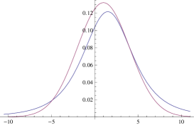
(b) Prior marginal density of $Z_{1}$ is normal with mean=1 and variance=9.1. Posterior density has mean (and mode) 1.5 and heavier tails .

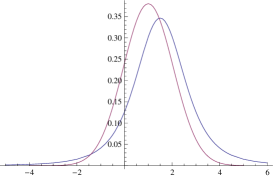
(c) Prior marginal density of $Z_{2}$ is normal with mean=1 and variance=1.1. Posterior density has mean (and mode) 1.5 and heavier tails.

Figure 1: Prior and posterior marginal densities under a constraint on the marginal density of a portfolio.

In Figure 1 we compare the marginal densities of $X$, $Z_{1}$ and $Z_{2}$ under prior and posterior distributions. We note that incorporating the constraint that $X$ has a fat-tailed density renders the asset returns from $A_{1}$ and $A_{2}$ to be similarly fat-tailed.

Example 2.

We consider an equally weighted portfolio in six global indices: ASX (the S$\&$P/ASX200, Australian stock index), DAX (the German stock index), EEM (the MSCI emerging market index), FTSE (the FTSE100, London Stock Exchange), Nikkei (the Nikkei225, Tokyo Stock Exchange) and S$\&$P (the Standard and Poor 500). Let $Z_{1},Z_{2},\ldots,Z_{6}$ denote the weekly rate of returns from ASX, DAX, EEM, FTSE, Nikkei and S$\&$P, respectively. We take prior distribution of $(Z_{1},Z_{2},\ldots,Z_{6})$ to be multivariate Gaussian with mean vector

$$[0.062\%\quad 0.28\%\quad 0.045\%\quad 0.13\%\quad 0.24\%\quad 0.26\%]$$

and variance-covariance matrix

$$\left(\begin{array}[]{cccccc}0.4285&0.4018&0.4394&0.3550&0.0269&0.3194\\ 0.4018&0.8139&0.6542&0.5353&0.0558&0.5274\\ 0.4394&0.6542&0.9278&0.5248&0.0060&0.5486\\ 0.3550&0.5353&0.5248&0.4791&0.0371&0.4220\\ 0.0269&0.0558&0.0060&0.0371&0.7606&0.0420\\ 0.3194&0.5274&0.5486&0.4220&0.0420&0.4801\end{array}\right)\times 10^{-3}$$

estimated from the historical prices of these indices (over the period Jan 2010 to Dec 2013). Assuming a notional amount of 1 million, the historical value-at-risk (VaR) and VaR under the prior distribution for our portfolio for different confidence levels are reported, respectively, in the second and third column of Table 1. Next, suppose that we expect the indices ASX, EEM and S$\&$P to strengthen and have expected weekly rates of return as $0.1\%,0.1\%\text{ and }0.35\%$ respectively. Further, consider an independent expert view that returns on DAX will exhibit a heavy-tailed behaviour. Specifically, let the expert views be:

• $\tilde{E}Z_{1}=0.1\%,\tilde{E}Z_{3}=0.1\%,\tilde{E}Z_{4}=0.13\%,\tilde{E}Z_{5}=0.24\%,\tilde{E}Z_{6}=0.35\%$ and

• $Z_{2}$ has a $t$-distribution with 3 degrees of freedom.

The fourth column in Table 1 reports VaRs at different confidence levels under the posterior distribution obtained after incorporating views only on expected returns (that xzis, only View (a)). We see that these do not differ much from those under the prior distribution. This can be contrasted with the fifth column where we have reported the VaRs (computed from 100,000 samples) under the posterior distribution obtained after including View (b) that $Z_{2}$ has $t$-distribution as well as the View (a) on the expected rates of return.

VaR at	Historical VaR	Prior distribution	Posterior with View (a)	Posterior with Views (a) and (b)	Posterior with Views (a) and (c)
0.9975	67,637	56,402	56,705	79,549	67,860
0.9950	56,048	51,895	52,198	63,301	58,416
0.9925	45,524	49,099	49,402	55,853	54,067
0.9500	29,682	33,746	34,049	29,544	33,080
0.7500	13,794	14,829	15,312	12,163	13,970
0.5000	2,836	1,680	2,983	1,968	2,078

Table 1: The second column reports VaR obtained from historical returns and the third column reports VaR under the prior multivariate normal distribution. While the fourth column is for VaR from posterior distribution after including view on expected returns (that is, View (a)) the fifth and sixth columns corresponds to VaR from posterior distribution after incorporating views both on density and expected returns

Next, suppose that we have the assumption of heavy-tailed density on returns of a different asset rather than DAX; for example, consider the following view:

• A $t$-distribution models returns on S$\&$P better. Specifically, let us say that a $t$-distribution with 6 degrees of freedom is more representative of the tail behaviour of observed values of $Z_{6}.$

The VaRs corresponding to the posterior distribution obtained after incorporating Views (a) and (c) are reported in Column 6 of Table 1. It can be observed from Columns 5 and 6 of Table 1 that unlike posterior distribution which includes views only on expected rates of return, marked differences occur from prior VaRs if heavy-tailed distribution is assumed for any component asset.

5 Applications to Options Pricing

In this section, we consider an options pricing scenario where the implied risk neutral densities of certain highly liquid assets can be used as views to calibrate models for pricing options written over assets that may be less actively traded but correlated with the liquid assets. We show that such views on densities get easily incorporated through our optimization problem $\bf{O_{1}}.$

In the option pricing scenario, an effective way to price an option is through evaluating its expected payoff with respect to the risk neutral density implied by the option prices observed in the market. However, as discussed in [5], estimating implied risk neutral densities require availability of data over a large number of strikes. There exists a huge body of literature on extracting implied risk neutral density from observed option prices of highly liquid stocks that are traded at many strikes (see [14] for a comprehensive review). However, for a stock which is not actively traded, estimation of implied risk neutral density is difficult, and in such cases, the implied risk neutral density available for some heavily traded benchmark asset which is representative of the market and correlated with the stock of our interest can be posed as a view/constraint on the marginal distribution. This view can then be incorporated in the prior Black-Scholes model to arrive at a posterior model which is more representative of the observed options prices. To illustrate the applicability of our framework to the option pricing problem, we provide an example here.

Example 3.

Consider the problem of pricing an out of the money call option on IBM stock trading at USD 82.98 on Jan 5, 2005. This option with strike at USD 88 is set to expire after 72 days, that is on March 18, 2005. The annual risk free interest rate is $2.69\%.$ We may have further relevant additional information in the market: For example, if there is an in the money option at strike price USD 80 on the same IBM stock for the same maturity which is traded heavily at USD 4.53, this additional information presents itself as the following constraint on risk neutral density:

$$e^{-D}\mathbb{E}[(X-80)^{+}]=4.53,$$ (8)

where $X$ is the value of IBM stock at maturity, $D$ is the discount factor and $\mathbb{E}[\cdot]$ is the expectation operator with respect to the risk neutral measure. Further, it is easy to obtain the daily closing bid and ask prices for some highly liquid instruments like Standard and Poor’s 500 Index options. S&P500 index is widely accepted as the proxy for U.S. market portfolio. As mentioned in the Introduction, its risk neutral density implied by the traded options encompasses information that can be expressed via constraints on expectations (like option prices, mean rate of return, etc.) and much more (like market sentiments, risk preferences, sensitivity to new information, etc.); see [12] for a detailed discussion on this. The S&P500 option price data and the risk free rate that we use are from Table 1 in [12] (this facilitates in utilizing the same implied risk neutral density extracted from the option prices in [12]). Let $Y$ denote the value of S&P500 index at maturity and $g_{\textnormal{rnd}}(\cdot)$ denote the risk neutral density of $Y$ implied by the option prices. Then the following constraint gets imposed on the joint risk neutral density $f_{X,Y}(\cdot,\cdot)$:

$$\int f_{X,Y}(x,y){\mathnormal{d}}x=g_{\textnormal{rnd}}(y),\text{ for all }y.$$ (9)

For computing the prior joint risk neutral density, we calibrate multi-asset Black-Scholes model from the historical data of IBM and S&P500 prior to Jan 5, 2005 obtained from Yahoo Finance. This results in a normal prior with covariance matrix

$$\begin{bmatrix}3.969&-0.4721\\ -0.4721&4.489\end{bmatrix}\times 10^{-5}$$

on log-returns of the IBM stock and S&P500 index respectively. The overall problem naturally manifests into finding a posterior density close to the specified risk neutral lognormal prior $f(\cdot,\cdot)$ while satisfying constraints (8) and (9). From Theorem 2, the posterior joint risk neutral density $f_{\textnormal{pos}}(\cdot,\cdot)$ is of the following form:

$$f_{\textnormal{pos}}(x,y)=e^{\lambda(x-80)^{+}}f(x|y)g_{\textnormal{rnd}}(y),$$

where $\lambda$ solving

$$\int_{x,y}(x-80)^{+}e^{\lambda(x-80)^{+}}f(x|y)g_{\textnormal{rnd}}(y){\mathnormal{d}}x{\mathnormal{d}}y=4.53e^{D}$$

is found to be 0.2479 numerically. This can then be used to compute the price of the out of the money IBM option with strike at USD 88 as below:

$$e^{-D}\int_{x,y}(x-88)^{+}e^{0.2479(x-80)^{+}}f(x|y)g_{\textnormal{rnd}}(y){\mathnormal{d}}x{\mathnormal{d}}y=1.17.$$

It is easy to incorporate additional option price constraints as in (8) and find a posterior risk neutral density that is consistent with all the observed option prices along with the implied marginal risk neutral density.

6 Conclusion

In this article, we built upon the existing methodologies that use relative entropy based ideas for incorporating mathematically specified views/constraints to a given financial model to arrive at a more accurate one. Our key contribution is that we extend the proposed methodology to allow for constraints on marginal distributions of functions of underlying variables in addition to moment constraints. In addition, we specialized our results to the Markowitz portfolio modeling framework where multivariate Gaussian distribution is used to model asset returns. Here, we developed closed-form solutions for the updated posterior distribution. In case when there is a constraint that a marginal of a single portfolio of assets has a fat-tailed distribution, we showed that under the posterior distribution, marginal of all assets with non-zero correlation with this portfolio have similar fat-tailed distribution. This may be a reasonable and a simple way to incorporate realistic tail behavior in a portfolio of assets. We also illustrated an application of the proposed framework in option pricing setting. Finally, we numerically tested the proposed methodology on simple examples.

Acknowledgement: The authors would like to thank Paul Glasserman for directional suggestions that greatly helped this effort.

Appendix: Proofs

Here we provide proofs of Theorem 2, Proposition 1 and Theorem 3.

Proof of Theorem 2:   Let $F:\mathbb{R}^{k}\rightarrow\mathbb{R}$ be a function defined as

$$F(\mbox{\boldmath{$\lambda$}})=\int_{\mathbb{x}}\log\left(\int_{\mathbb{y}}\exp\left(\sum_{l}\lambda_{l}h_{l}(\mathbb{x},\mathbb{y})\right)f(\mathbb{y}|\mathbb{x})d\mathbb{y}\right)g(\mathbb{x})d\mathbb{x}-\sum_{l}\lambda_{l}c_{l}.$$

Then,

$$\frac{\partial F}{\partial\lambda_{i}} = \int_{\mathbb{x}}\left(\frac{\int_{\mathbb{y}}h_{i}(\mathbb{x},\mathbb{y})\exp\left(\sum_{l}\lambda_{l}h_{l}(\mathbb{x},\mathbb{y})\right)f(\mathbb{y}|\mathbb{x})d\mathbb{y}}{\int_{\mathbb{y}}\exp\left(\sum_{l}\lambda_{l}h_{l}(\mathbb{x},\mathbb{y})\right)f(\mathbb{y}|\mathbb{x})d\mathbb{y}}\right)g(\mathbb{x})d\mathbb{x}-c_{i}$$

$$= \int_{\mathbb{x}}\left(\int_{\mathbb{y}}h_{i}(\mathbb{x},\mathbb{y})\frac{\exp\left(\sum_{l}\lambda_{l}h_{l}(\mathbb{x},\mathbb{y})\right)f(\mathbb{y}|\mathbb{x})}{\int_{\mathbb{y}}\exp\left(\sum_{l}\lambda_{l}h_{l}(\mathbb{x},\mathbb{y})\right)f(\mathbb{y}|\mathbb{x})d\mathbb{y}}\,d\mathbb{y}\right)g(\mathbb{x})d\mathbb{x}-c_{i}$$

$$= \int_{\mathbb{x}}\left(\int_{\mathbb{y}}h_{i}(\mathbb{x},\mathbb{y})f_{\mbox{\boldmath{$\lambda$}}}(\mathbb{y}|\mathbb{x})d\mathbb{y}\right)g(\mathbb{x})d\mathbb{x}-c_{i}$$

$$= \int_{\mathbb{x}}\int_{\mathbb{y}}h_{i}(\mathbb{x},\mathbb{y})f_{\mbox{\boldmath{$\lambda$}}}(\mathbb{x},\mathbb{y})d\mathbb{x}d\mathbb{y}-c_{i}$$

$$= \mathbb{E}_{\mbox{\boldmath{$\lambda$}}}[h_{i}(\mathbb{X},\mathbb{Y})]-c_{i}.$$

Hence the set of equations given by $\mathbb{E}_{\mbox{\boldmath{$\lambda$}}}[h_{i}(\mathbb{X},\mathbb{Y})]=c_{i},i=1,\ldots,k$ is equivalent to:

$$\left(\frac{\partial F}{\partial\lambda_{1}},\frac{\partial F}{\partial\lambda_{2}},\ldots,\frac{\partial F}{\partial\lambda_{k}}\right)=0\,.$$ (10)

The solution to this set of equations exist when the prior model is such that

$$\nabla\log\mathbb{E}\left[\exp\left(\sum_{l=1}^{k}\lambda_{l}h_{l}(\bf{X,Y})\right)\right]=(c_{1},\ldots,c_{k})^{T},$$

for some $\lambda=(\lambda_{1},\ldots,\lambda_{k})$ in $\mathbb{R}^{k}.$ Since

$$\frac{\partial}{\partial\lambda_{j}}f_{\mbox{\boldmath{$\lambda$}}}(\mathbb{y}|\mathbb{x})=h_{j}(\mathbb{x},\mathbb{y})f_{\mbox{\boldmath{$\lambda$}}}(\mathbb{y}|\mathbb{x})-\left(\int_{\mathbb{y}}h_{j}(\mathbb{x},\mathbb{y})f_{\mbox{\boldmath{$\lambda$}}}(\mathbb{y}|\mathbb{x})d\mathbb{y}\right)\times f_{\mbox{\boldmath{$\lambda$}}}(\mathbb{y}|\mathbb{x}),$$

we have

$$\frac{\partial^{2}F}{\partial\lambda_{j}\partial\lambda_{i}} = \int_{\mathbb{x}}\left(\int_{\mathbb{y}}h_{i}(\mathbb{x},\mathbb{y})\frac{\partial}{\partial\lambda_{j}}f_{\mbox{\boldmath{$\lambda$}}}(\mathbb{y}|\mathbb{x})\,d\mathbb{y}\right)g(\mathbb{x})\,d\mathbb{x}$$

$$= \int_{\mathbb{x}}\left(\int_{\mathbb{y}}h_{i}(\mathbb{x},\mathbb{y})h_{j}(\mathbb{x},\mathbb{y})f_{\mbox{\boldmath{$\lambda$}}}(\mathbb{y}|\mathbb{x})d\mathbb{y}\right)g(\mathbb{x})d\mathbb{x}$$

$$-\int_{\mathbb{x}}\left(\int_{\mathbb{y}}h_{j}(\mathbb{x},\mathbb{y})f_{\mbox{\boldmath{$\lambda$}}}(\mathbb{y}|\mathbb{x})d\mathbb{y}\right)\left(\int_{\mathbb{y}}h_{i}(\mathbb{x},\mathbb{y})f_{\mbox{\boldmath{$\lambda$}}}(\mathbb{y}|\mathbb{x})d\mathbb{y}\right)g(\mathbb{x})d\mathbb{x}$$

$$= \mathbb{E}_{g(\mathbb{x})}\left[\mathbb{E}_{\mbox{\boldmath{$\lambda$}}}[h_{i}(\mathbb{X},\mathbb{Y})h_{j}(\mathbb{X},\mathbb{Y})\mid\mathbb{X}]\right]-\mathbb{E}_{g(\mathbb{x})}\left[\mathbb{E}_{\mbox{\boldmath{$\lambda$}}}[h_{j}(\mathbb{X},\mathbb{Y})\mid\mathbb{X}]\times\mathbb{E}_{\mbox{\boldmath{$\lambda$}}}[h_{i}(\mathbb{X},\mathbb{Y})\mid\mathbb{X}]\right]$$

$$= \mathbb{E}_{g(\mathbb{x})}\left[\text{Cov}_{\mbox{\boldmath{$\lambda$}}}[h_{i}(\mathbb{X},\mathbb{Y}),h_{j}(\mathbb{X},\mathbb{Y})\mid\mathbb{X}]\right],$$

where $E_{g(\mathbb{x})}$ denote expectation with respect to the density function $g(\mathbb{x})$. By our assumption, it follows that the Hessian of $F(\cdot)$ is positive definite. Thus, the function $F(\cdot)$ is strictly convex in $\mathbb{R}^{k}$. Therefore if there exists a solution to (10), then it is unique. Since (10) is equivalent to our constraints that $\mathbb{E}_{\mbox{\boldmath{$\lambda$}}}[h_{i}(\mathbb{X},\mathbb{Y})]=c_{i},$ the theorem follows. $\Box$

Proof of Proposition 1:   By Theorem 1, $\tilde{f}(\mathbb{x},\mathbb{y})=g(\mathbb{x})\times\tilde{f}(\mathbb{y}|\mathbb{x}),$ where

$$\tilde{f}(\mathbb{y}|\mathbb{x})=\frac{e^{\mbox{\boldmath{$\lambda$}}^{T}\mathbb{y}}f(\mathbb{y}|\mathbb{x})}{\int e^{\mbox{\boldmath{$\lambda$}}^{T}\mathbb{y}}f(\mathbb{y}|\mathbb{x})d\mathbb{y}}.$$

Here the superscript $T$ corresponds to the transpose. Now $f(\mathbb{y}|\mathbb{x})$ is the $k$-variate normal density with mean vector $\mbox{\boldmath{$\mu$}}_{\mathbb{y}|\mathbb{x}}=\mbox{\boldmath{$\mu$}}_{\mathbb{y}}+\mathbb{\Sigma}_{\mathbb{yx}}\mathbb{\Sigma}_{\mathbb{xx}}^{-1}(\mathbb{x}-\mbox{\boldmath{$\mu$}}_{\mathbb{x}})$ and the variance-covariance matrix $\mathbb{\Sigma}_{\mathbb{y}|\mathbb{x}}=\mathbb{\Sigma}_{\mathbb{yy}}-\mathbb{\Sigma}_{\mathbb{yx}}\mathbb{\Sigma}_{\mathbb{xx}}^{-1}\mathbb{\Sigma}_{\mathbb{xy}}.$ Hence $\tilde{f}(\mathbb{y}|\mathbb{x})$ is the normal density with mean $(\mbox{\boldmath{$\mu$}}_{\mathbb{y}|x}+\mathbb{\Sigma}_{\mathbb{y}|\mathbb{x}}\mbox{\boldmath{$\lambda$}})$ and variance-covariance matrix $\mathbb{\Sigma}_{\mathbb{y}|\mathbb{x}}$. Now the moment constraint equation (4) implies:

$$\mathbb{a} = \int_{\mathbb{x}\in\mathbb{R}^{N-k}}\int_{\mathbb{y}\in\mathbb{R}^{k}}\mathbb{y}\tilde{f}(\mathbb{x},\mathbb{y})d\mathbb{y}d\mathbb{x}$$

$$= \int_{\mathbb{x}\in\mathbb{R}^{N-k}}g(\mathbb{x})\left(\int_{\mathbb{y}\in\mathbb{R}^{k}}\mathbb{y}\tilde{f}(\mathbb{y}|\mathbb{x})d\mathbb{y}\right)d\mathbb{x}$$

$$= \int_{\mathbb{x}\in\mathbb{R}^{N-k}}g(\mathbb{x})\left(\mbox{\boldmath{$\mu$}}_{\mathbb{y}|\mathbb{x}}+\mathbb{\Sigma}_{\mathbb{y}|\mathbb{x}}\mbox{\boldmath{$\lambda$}}\right)d\mathbb{x}$$

$$= \int_{\mathbb{x}\in\mathbb{R}^{N-k}}g(\mathbb{x})\left(\mbox{\boldmath{$\mu$}}_{\mathbb{y}}+\mathbb{\Sigma}_{\mathbb{yx}}\mathbb{\Sigma}_{\mathbb{xx}}^{-1}(\mathbb{x}-\mbox{\boldmath{$\mu$}}_{\mathbb{x}})+\mathbb{\Sigma}_{\mathbb{y}|\mathbb{x}}\mbox{\boldmath{$\lambda$}}\right)d\mathbb{x}$$

$$= \mbox{\boldmath{$\mu$}}_{\mathbb{y}}+\mathbb{\Sigma}_{\mathbb{yx}}\mathbb{\Sigma}_{\mathbb{xx}}^{-1}(\mathbb{E}_{g}[\mathbb{X}]-\mbox{\boldmath{$\mu$}}_{\mathbb{x}})+\mathbb{\Sigma}_{\mathbb{y}|\mathbb{x}}\mbox{\boldmath{$\lambda$}}.$$

Therefore, to satisfy the moment constraint, we must take

$$\mbox{\boldmath{$\lambda$}}=\mathbb{\Sigma}_{\mathbb{y}|\mathbb{x}}^{-1}\left[\mathbb{a}-\mbox{\boldmath{$\mu$}}_{\mathbb{y}}-\mathbb{\Sigma}_{\mathbb{yx}}\mathbb{\Sigma}_{\mathbb{xx}}^{-1}(\mathbb{E}_{g}[\mathbb{X}]-\mbox{\boldmath{$\mu$}}_{\mathbb{x}})\right]\,.$$

Putting the above value of $\lambda$ in $(\mbox{\boldmath{$\mu$}}_{\mathbb{y}|\mathbb{x}}+\mathbb{\Sigma}_{\mathbb{y}|\mathbb{x}}\mbox{\boldmath{$\lambda$}})$ we see that $\tilde{f}(\mathbb{y}|\mathbb{x})$ is the normal density with mean $\mathbb{a}+\mathbb{\Sigma}_{\mathbb{yx}}\mathbb{\Sigma}_{\mathbb{xx}}^{-1}(\mathbb{x}-E_{g}[\mathbb{X}])$ and variance-covariance matrix $\mathbb{\Sigma}_{\mathbb{y}|\mathbb{x}}.$ $\Box$

Proof of Theorem 3:   We have

$$\tilde{f}(\mathbb{y}|x)=D\exp\left(-\frac{1}{2}(\mathbb{y}-\tilde{\mbox{\boldmath{$\mu$}}}_{\mathbb{y}|x})^{t}\mathbb{\Sigma}_{\mathbb{y}|x}^{-1}(\mathbb{y}-\tilde{\mbox{\boldmath{$\mu$}}}_{\mathbb{y}|x})\right)$$

for an appropriate constant $D$, where

$$\tilde{\mbox{\boldmath{$\mu$}}}_{\mathbb{y}|x}=\mathbb{a}+\left(\frac{x-E_{g}(X)}{\sigma_{xx}}\right)\mbox{\boldmath{$\sigma$}}_{x\mathbb{y}}.$$

Suppose that the stated assumptions hold for $i=1$. Under the optimal distribution, the marginal density of $Y_{1}$ is

$$\tilde{f}_{Y_{1}}(y_{1})=\int_{(x,y_{2},...,y_{k})}D\exp\left(-\frac{1}{2}(\mathbb{y}-\tilde{\mbox{\boldmath{$\mu$}}}_{\mathbb{y}|x})^{t}\mathbb{\Sigma}_{\mathbb{y}|x}^{-1}(\mathbb{y}-\tilde{\mbox{\boldmath{$\mu$}}}_{\mathbb{y}|x})\right)g(x)dxdy_{2}...dy_{k}.$$

Now the limit in (7) is equal to:

$$\lim_{y_{1}\to\infty}\int_{(x,y_{2},y_{3},...,y_{k})}D\exp\left(-\frac{1}{2}(\mathbb{y}-\tilde{\mbox{\boldmath{$\mu$}}}_{\mathbb{y}|x})^{t}\mathbb{\Sigma}_{\mathbb{y}|x}^{-1}(\mathbb{y}-\tilde{\mbox{\boldmath{$\mu$}}}_{\mathbb{y}|x})\right)\times\frac{g(x)}{g(y_{1})}dxdy_{2}...dy_{k}.$$

The term in the exponent is:

$$-\frac{1}{2}\sum_{i=1}^{k}\left(\mathbb{\Sigma}_{\mathbb{y}|x}^{-1}\right)_{ii}\left((y_{i}-a^{\prime}_{i})-x\frac{\sigma_{xy_{i}}}{\sigma_{xx}}\right)^{2}-\frac{1}{2}\sum_{i\neq j}\left(\mathbb{\Sigma}_{\mathbb{y}|x}^{-1}\right)_{ij}\left((y_{i}-a^{\prime}_{i})-x\frac{\sigma_{xy_{{}_{i}}}}{\sigma_{xx}}\right)\left((y_{j}-a^{\prime}_{j})-x\frac{\sigma_{xy_{{}_{j}}}}{\sigma_{xx}}\right)$$

where $a^{\prime}_{i}=a_{i}-{E_{g}(X)}\sigma_{xy_{i}}/{\sigma_{xx}}.$ Now we make the following substitutions:

$$(x,y_{2},y_{3},...,y_{k})\longmapsto\mathbb{y}^{\prime}=(y_{1}^{\prime},y_{2}^{\prime},y_{3}^{\prime},...,y_{k}^{\prime}),$$

$$y_{1}^{\prime}=(y_{1}-a^{\prime}_{1})-x\frac{\sigma_{xy_{{}_{1}}}}{\sigma_{xx}},\text{ and }y_{i}^{\prime}=(y_{i}-a^{\prime}_{i})-x\frac{\sigma_{xy_{{}_{i}}}}{\sigma_{xx}},i=2,3,...,k.$$

Assuming that $\sigma_{xy_{{}_{1}}}=\textnormal{Cov}(X,Y_{1})\neq 0$, the inverse map $\mathbb{y}^{\prime}=(y_{1}^{\prime},y_{2}^{\prime},y_{3}^{\prime},...,y_{k}^{\prime})\longmapsto(x,y_{2},y_{3},...,y_{k})$ is given by:

$$x=\frac{\sigma_{xx}}{\sigma_{xy_{1}}}(y_{1}-y^{\prime}_{1}-a^{\prime}_{1}),\quad\quad y_{i}=y^{\prime}_{i}+a^{\prime}_{i}+\frac{\sigma_{xy_{i}}}{\sigma_{xy_{1}}}(y_{1}-y^{\prime}_{1}-a^{\prime}_{1})\text{ for }i=2,3,...,k,$$

$$\text{with Jacobian}\ \ \left|\det\left(\frac{\partial(x,y_{2},y_{3},...,y_{k})}{\partial(y_{1}^{\prime},y_{2}^{\prime},y_{3}^{\prime},...,y_{k}^{\prime})}\right)\right|=\frac{\sigma_{xx}}{\sigma_{xy_{{}_{1}}}}.$$

The integrand then becomes

$$D\exp\left(\frac{1}{2}{\mathbb{y}^{\prime}}^{T}\mathbb{\Sigma}_{\mathbb{y}|x}^{-1}\mathbb{y}^{\prime}\right)\frac{g\left(\frac{\sigma_{xx}}{\sigma_{xy_{{}_{1}}}}(y_{1}-y^{\prime}_{1}-a^{\prime}_{1})\right)}{g(y_{1})}\frac{\sigma_{xx}}{\sigma_{xy_{{}_{1}}}}.$$

By assumption,

$$\frac{g\left(\frac{\sigma_{xx}}{\sigma_{xy_{1}}}(y_{1}-y^{\prime}_{1}-a^{\prime}_{1})\right)}{g(y_{1})}\leq h(y_{1})\,\,\text{for all}\,y_{1},$$

for some non-negative function $h(\cdot)$ such that $Eh(Z)<\infty$ when $Z$ has a Gaussian distribution. Therefore, by dominated convergence theorem, we have that

$$\lim_{y_{1}\to\infty} \int{D\exp\left(-\frac{1}{2}{\mathbb{y}^{\prime}}^{T}\mathbb{\Sigma}_{\mathbb{y}|x}^{-1}\mathbb{y}^{\prime}\right)\frac{g\left(\frac{\sigma_{xx}}{\sigma_{xy_{{}_{1}}}}(y_{1}-y^{\prime}_{1}-a^{\prime}_{1})\right)}{g(y_{1})}\frac{\sigma_{xx}}{\sigma_{xy_{{}_{1}}}}d\mathbb{y}^{\prime}}$$

$$= \int D\exp\left(-\frac{1}{2}{\mathbb{y}^{\prime}}^{T}\mathbb{\Sigma}_{\mathbb{y}|x}^{-1}\mathbb{y}^{\prime}\right)\lim_{y_{1}\to\infty}\frac{g\left(\frac{\sigma_{xx}}{\sigma_{xy_{{}_{1}}}}(y_{1}-y^{\prime}_{1}-a^{\prime}_{1})\right)}{g(y_{1})}\frac{\sigma_{xx}}{\sigma_{xy_{{}_{1}}}}d\mathbb{y}^{\prime}$$

$$= \int D\exp\left(-\frac{1}{2}{\mathbb{y}^{\prime}}^{T}\mathbb{\Sigma}_{\mathbb{y}|x}^{-1}\mathbb{y}^{\prime}\right)\lim_{y_{1}\to\infty}\frac{g\left(\frac{\sigma_{xx}}{\sigma_{xy_{{}_{1}}}}(y_{1}-y^{\prime}_{1}-a^{\prime}_{1})\right)}{g(y_{1}-y^{\prime}_{1}-a^{\prime}_{1})}\lim_{y_{1}\to\infty}\frac{g(y_{1}-y^{\prime}_{1}-a^{\prime}_{1})}{g(y_{1})}\frac{\sigma_{xx}}{\sigma_{xy_{{}_{1}}}}d\mathbb{y}^{\prime},$$

which, by our assumption on $g(\cdot)$, in turn equals

$$\int D\exp\left(-\frac{1}{2}{\mathbb{y}^{\prime}}^{T}\mathbb{\Sigma}_{\mathbb{y}|x}^{-1}\mathbb{y}^{\prime}\right)\times\left(\frac{\sigma_{xy_{1}}}{\sigma_{xx}}\right)^{\alpha}\times 1\times\frac{\sigma_{xx}}{\sigma_{xy_{1}}}d\mathbb{y}^{\prime}=\left(\frac{\sigma_{xy_{{}_{1}}}}{\sigma_{xx}}\right)^{\alpha-1}\,\,.\,\,\quad\quad\quad\quad\Box$$

References

• [1] M. Avellaneda. Minimum entropy calibration of asset-pricing models. International Journal of Theoretical and Applied Finance., 1:447–472, 1998.
• [2] M. Avellaneda, R. Buff, C. Friedman, N. Grandchamp, L. Kruk, and J. Newman. Weighted monte carlo: A new technique for calibrating asset pricing models. International Journal of Theoretical and Applied Finance., 4(1):91–119, March 2001.
• [3] M. Avellaneda, C. Friedman, R. Holmes, and D. Samperi. Calibrating volatility surfaces via relative entropy minimization. Applied Mathematical Finance., 4(1):37–64, March 1997.
• [4] F. Black and R. Litterman. Asset allocation: combining investor views with market equilibrium. Goldman Sachs Fixed Income Research, 1990.
• [5] D. T. Breeden and R. H. Litzenberger. Prices of state-contingent claims implicit in option prices. Journal of business, pages 621–651, 1978.
• [6] P. Buchen and M. Kelly. The maximum entropy distribution of an asset inferred from option prices. The Journal of Financial and Quantitative Analysis., 31(1):143–159, March 1996.
• [7] T. Cover and J. Thomas. Elements of Information Theory. John Wiley and Sons, Wiley series in Telecommunications, 1999.
• [8] I. Csiszar. I-divergence geometry of probability distribution and minimization problems. Annals of Probability, 3(1):146–158, 1975.
• [9] A. Dembo and O. Zeitouni. Large Deviations Techniques and Applications. Springer, Application of mathematics-38, 1998.
• [10] P. Dupuis and R. Ellis. A Weak Convergence Approach to the Theory of Large Deviations. Wiley, Wiley series in probability and statistics, 1986.
• [11] W. Feller. An Introduction to Probability Theory and its Applications,Vol-2. John Wiley and Sons Inc., New York, 1971.
• [12] S. Figlewski. Estimating the Implied Risk Neutral Density. Volatility and Time Series Econometrics: Essays in Honor of Robert Engle. Oxford University Press, 2009.
• [13] P. Glasserman and B. Yu. Large sample properties of weighted monte carlo estimators. Operation Research, 53(2):298–312, 2005.
• [14] J. C. Jackwerth. Option-implied risk-neutral distributions and risk aversion. Research Foundation of AIMR Charlotteville, 2004.
• [15] Y. Kitamura and M. Stutzer. Entropy-based estimation methods. In Encyclopedia of Quantitative Finance, pages 567–571. Wiley, 2010.
• [16] A. Meucci. Fully flexible views: theory and practice. Risk, 21(10):97–102, 2008.
• [17] J. Mina and J. Xiao. Return to riskmetrics: the evolution of a standard. RiskMatrics publications, 2001.
• [18] J. Pazier. Global portfolio optimization revisited: a least discrimination alternative to black-litterman. ICMA Centre Discussion Papers in Finance, July 2007.
• [19] E. Qian and S. Gorman. Conditional distribution in portfolio theory. Financial analyst journal., 57(2):44–51, March-April 1993.
• [20] M. Stutzer. A simple non-parametric approach to derivative security valuation. Journal of Finance, 101(5):1633–1652, 1997.