Quantized recurrence time in iterated open quantum dynamics

Abstract

The expected return time to the original state is a key concept characterizing systems obeying both classical or quantum dynamics. We consider iterated open quantum dynamical systems in finite dimensional Hilbert spaces, a broad class of systems that includes classical Markov chains and unitary discrete time quantum walks on networks. Starting from a pure state, the time evolution is induced by repeated applications of a general quantum channel, in each timestep followed by a measurement to detect whether the system has returned to the original state. We prove that if the superoperator is unital in the relevant Hilbert space (the part of the Hilbert space explored by the system), then the expectation value of the return time is an integer, equal to the dimension of this relevant Hilbert space. We illustrate our results on partially coherent quantum walks on finite graphs. Our work connects the previously known quantization of the expected return time for bistochastic Markov chains and for unitary quantum walks, and shows that these are special cases of a more general statement. The expected return time is thus a quantitative measure of the size of the part of the Hilbert space available to the system when the dynamics is started from a certain state.

I Introduction

An important task in physics is to observe the dynamics of systems and predict their future behavior. Monitoring the evolution of a classical system does not alter its dynamics in the ideal case; in quantum mechanics, however, frequent measurements may have dramatic effects due to the measurement back-action, e.g., freezing the dynamics, as in the quantum Zeno effect Mack et al. (2014); Chandrashekar (2010a), or losing coherence and thereby arriving at classical-like behaviorJoos (2003). The problem becomes even more complicated under realistic conditions, where the effects of the environment cannot be neglected and the introduced noise affects the fine quantum features needed for applications, e.g. in quantum informationLidar and Brun (2013).

Discretization, both in time and space, is inherent in the definition of many physical systems (e.g., networks), but can also occur as a result of an approximation to make a system numerically tractable. Iterations of a given generic time evolution step and assuming a countable number of different states of the system thus represents a large class of physical situations, including classical and quantum networksPerseguers et al. (2013). A generic way to represent a discretized iterative dynamical process, is a discrete time random walk on a graph, in both the classical and the quantum case.

Discrete-time quantum walks (DTQW)Venegas-Andraca (2012), quantum mechanical generalizations of random walks, have in the recent years enjoyed increasing attention from both theoretical and experimental Schreiber et al. (2010); Karski et al. (2009); Genske et al. (2013); Sansoni et al. (2012); Broome et al. (2010); Zähringer et al. (2010); Schreiber et al. (2011) physicists. The hallmark property of DTQWs is that they spread faster than classical random walks: on a regular graph, the variance of the position of the walker scales as $\mathcal{O}(t^{2})$ with the number $t$ of timesteps, rather than $\mathcal{O}(t)$ as in the classical case. This gives quantum search algorithms using DTQWsShenvi et al. (2003) the same quadratic speedup as possessed by the celebrated Grover algorithmGrover (1996) – all the more important since DTQWs can be used to implement universal quantum computation Lovett et al. (2010). Characterization of quantum walks using fundamental concepts might not only further our understanding of when and how the quantum speedup arises, but can also lead to new types of algorithms based on DTQWs.

One of the important concepts used to characterize iterative dynamical processes, such as random walks on graphs, is recurrence: whether a system returns to its initial state, and if so, how long this return takes. For finite, closed systems (where the dynamics conserves the phase-space volume), the Poincaré theorem guarantees that recurrence does take place, although the required time can be beyond the range of any conceivable experiment. The problem of this return time in classicalBarreira (2005) and quantum systems Casati et al. (1999) is an important question for many areas of physics, from chaos theory to the microscopic foundations of thermodynamics.

There is a broad class of classical iterative dynamical processes for which the recurrence time, i.e., the expected return time to an initial state $j$, turns out to be quantized, i.e., an integer $T_{j}$. This is the class of bistochastic processes, for which the completely mixed state is a stationary stateKemeny and Snell (1960). In this case, for each initial state $j$ the set $G_{j}$ of sites that are reachable from $j$ by iterations of the timestep form an irreducible component (all states in $G_{j}$, and only states in $G_{j}$ are reachable from each other). Since the process is bistochastic, in this irreducible component the uniform distribution is a stationary state. Consider now a trajectory of $N$ steps, started from state $j$, with $N\to\infty$; the number of times site $j$ is visited tends to $N/\left|{G_{j}}\right|$, where $\left|{G_{j}}\right|$ denotes the number of states in $G_{j}$. The average return time to state $j$ is the average time delay between such visits, which is $T_{j}=\left|{G_{j}}\right|$.

Generalizing the concept of the first return time to iterative quantum dynamical processes, Grünbaum et al.Grünbaum et al. (2013) have found a striking fact: its expectation value is quantized. To define a first return time, they suggested that every timestep, given by a unitary operator $U$, be followed by a measurement to detect whether the walker has returned to the initial state or not. Starting the system from a state $|{\Psi}\rangle$, they have found that the expected return time $T_{\Psi}$ is the dimension of the smallest eigenspace of $U$ that includes $|{\Psi}\rangle$, which is always an integer number, or infinity. Thus, the integer $T_{\Psi}$ is a measure of the size of the system accessible from the initial state, reminiscent of the classical case. This similarity is all the more surprising given that the proof of Grünbaum et al. is an intricate application of topological concepts to quantum physics.

In the present work, we address the problem of the recurrence time for all iterative open quantum dynamical systems (IOQDS; a.k.a. quantum dynamical semigroupsCirillo and Ticozzi (2014)): a broad class of processes that includes as special cases both the unitary case of Ref. Grünbaum et al., 2013 and classical Markov chains. The timestep of one period thus includes interaction with an environment, which can be beneficial for transportPlenio and Huelga (2008); Rebentrost et al. (2009). The timestep is defined by an arbitrary quantum channel (trace preserving completely positive map), represented by a superoperator $\mathcal{S}$, which is followed by a measurement to decide whether the system has returned or not. This iterated evolution can also be viewed as a generalized, open discrete time quantum walk Attal et al. (2012); Lardizabal and Souza (2014). We prove that whenever the timestep superoperator is unital, i.e., whenever the completely mixed state is a stationary state, $\mathcal{S}[\mathbb{I}]=\mathbb{I}$, the expected return time $T_{\Psi}$ to a pure state $|{\Psi}\rangle$ is an integer, equal to the dimension of the part of the Hilbert space that the system explores when started from $|{\Psi}\rangle$ (the relevant Hilbert space; more precisely, we only need $\mathcal{S}$ to be unital in this relevant Hilbert space).

This paper is structured as follows. In the next Section we fix the notation for iterated open quantum dynamical systems, i.e., generalized DTQWs, also introducing the concepts of the conditional density operators and of the relevant Hilbert space. In Section III we prove the main statement of our paper, that the expected return time for unital generalized DTQWs is equal to the dimension of the relevant Hilbert space. In Section IV we illustrate our results on DTQWs on finite graphs. Finally, we provide a short outlook on consequences of our results in Section V.

II First return time

We consider an iterated open quantum dynamical system, with dynamics that can be fully or partially coherent. The state is given by a time-dependent density operator $\rho:\mathcal{H}\to\mathcal{H}$ in a finite dimensional Hilbert space $\mathcal{H}$. The dynamics takes place in discrete time, $t\in\mathbb{N}$, starting from an initial pure state $|{\Psi}\rangle$,

$$\rho(0) =|{\Psi}\rangle\langle{\Psi}|,$$ (1)

and generated by a fixed superoperator $\mathcal{S}$. To describe a real physical process, $\mathcal{S}$ has to be trace preserving and completely positive (TPCP), i.e., a quantum channel. This is equivalent by the Stinespring–Kraus representation theorem Kraus et al. (1983) to the requirement that $\mathcal{S}$ can be written in terms of a discrete set of $D$ Kraus operators $A_{j}:\mathcal{H}\to\mathcal{H}$ as

$$\rho(t+1) =\mathcal{S}[\rho(t)]=\sum_{j=0}^{D-1}A_{j}\rho(t)A_{j}^{\dagger}.$$ (2)

The only restriction on the Kraus operators $A_{j}$ is the normalization condition

$$\sum_{j=0}^{D-1}A_{j}^{\dagger}A_{j}=\mathbb{I},$$ (3)

where $\mathbb{I}$ represents the unit operator on the whole Hilbert space $\mathcal{H}$.

II.1 Relevant Hilbert space

We can safely restrict our attention to the part of the Hilbert space that the system explores, started from $|{\Psi}\rangle$ and undergoing the iterations of $\mathcal{S}$. This is the relevant Hilbert space $\mathcal{H}_{\Psi}$, which we define via the limit of the series of projectors

$$\mathcal{\mathbb{I}}_{\Psi} =\lim_{n\to\infty}\text{supp}(\sum_{t=0}^{n}\rho(t)),$$ (4)

where $\text{supp}(\sigma)$ denotes the projector to the nonzero subspace (support) of a Hermitian operator $\sigma$. The relevant Hilbert space $\mathcal{H}_{\Psi}$ is the image of the operator $\mathcal{\mathbb{I}}_{\Psi}$ acting on $\mathcal{H}$.

The relevant Hilbert space $\mathcal{H}_{\Psi}$ is the smallest subspace of $\mathcal{H}$ that contains the state $|{\Psi}\rangle$ and fulfils the following property: for any positive semidefinite operator $\sigma:\mathcal{H}_{\Psi}\to\mathcal{H}_{\Psi}$, we have $\text{supp}(\mathcal{S}[\sigma])\subseteq\mathcal{H}_{\Psi}$. In the language of the Kraus operators of $\mathcal{S}$, as per Eq. (2), this reads that for all $j$, and any $|{\Phi}\rangle\in\mathcal{H}_{\Psi}$, we have $A_{j}|{\Phi}\rangle\in\mathcal{H}_{\Psi}$. These statements, proved in Appendix A, ensure that the restriction of the timestep operator $\mathcal{S}$ to the relevant Hilbert space, defined as

$$\mathcal{S}_{\Psi}[\rho]=\mathcal{S}[\mathcal{\mathbb{I}}_{\Psi}\rho\mathcal{\mathbb{I}}_{\Psi}]=\sum_{j=0}^{D-1}A_{j}\mathcal{\mathbb{I}}_{\Psi}\rho\mathcal{\mathbb{I}}_{\Psi}A_{j}^{\dagger},$$ (5)

for $\rho:\mathcal{H}\to\mathcal{H}$, can be used in place of $\mathcal{S}$ as long as we only consider an iterative quantum dynamics started from $|{\Psi}\rangle$. Since each of the Kraus operators map states from $\mathcal{H}_{\Psi}$ into states in $\mathcal{H}_{\Psi}$, the Kraus operators of $\mathcal{S}_{\Psi}$ are $A_{j}\mathcal{\mathbb{I}}_{\Psi}=\mathcal{\mathbb{I}}_{\Psi}A_{j}\mathcal{\mathbb{I}}_{\Psi}$.

The dimension of the relevant Hilbert space is equal to the trace of the projector $\mathcal{\mathbb{I}}_{\Psi}$,

$$\text{dim}(\mathcal{H}_{\Psi}) =\text{Tr}(\mathcal{\mathbb{I}}_{\Psi}).$$ (6)

The relevant Hilbert space is guaranteed to be finite dimensional if the full Hilbert space is finite dimensional.

II.2 Conditional dynamics

To define a first return time, we need to modify the dynamics and monitor whether the system returns to the initial state or not. At the end of every timestep, we perform a dichotomic measurement, with the projector corresponding to “return” given by $|{\Psi}\rangle\langle{\Psi}|$, and the projector of “no return” given by its complement, which acts on a general density operator $\sigma$ as

$$\mathcal{M}[\sigma] =(\mathbb{I}-|{\Psi}\rangle\langle{\Psi}|)\sigma(\mathbb{I}-|{\Psi}\rangle\langle{\Psi}|).$$ (7)

The first return time is the number of steps we need until we obtain “return”. The expected return time is the expectation value of this number.

A simple way to calculate the first return time in this monitored system is to use a conditional density operator $\rho_{\text{cond}}(t)$. This represents the state of the system under the condition that it has never returned to the origin. Using the superoperator $\mathcal{M}$ corresponding to “no return”, this conditional density operator reads

$$\rho_{\text{cond}}(t) =(\mathcal{M}\mathcal{S})^{t}[|{\Psi}\rangle\langle{\Psi}|]=(\mathcal{M}\mathcal{S}_{\Psi})^{t}[|{\Psi}\rangle\langle{\Psi}|],$$ (8)

for $t\in\mathbb{N}$, including $\rho_{\text{cond}}(0)=|{\Psi}\rangle\langle{\Psi}|$. The second equality above holds, since the projector $\mathcal{M}$ does not lead outside the relevant Hilbert space: for any positive semidefinite operator $\sigma$: $\mathcal{H}_{\Psi}\to\mathcal{H}_{\Psi}$, we have $\text{supp}(\mathcal{M}[\sigma])\subseteq\mathcal{H}_{\Psi}$, with $\mathcal{M}[\sigma]$ also positive semidefinite (but possibly $\text{Tr }(\mathcal{M}[\sigma])<\mathrm{Tr}\sigma$).

The trace of the conditional density operator $\rho_{\text{cond}}(t)$ is the probability $q_{t}$ that there was no return to the initial state up until time $t$,

$$q_{t} =\mathrm{Tr}\rho_{\text{cond}}(t).$$ (9)

We say that the dynamics is recurrent if this quantity converges to $0$.

II.3 Expected return time

In this paper we are interested in the expected return time $T_{\Psi}$, i.e., the expectation value of the first return time,

$$T_{\Psi} =\sum_{t=1}^{\infty}tp_{t},$$ (10)

where $p_{t}$ denotes the probability that the first return to $|{\Psi}\rangle$ happens at time $t$. We explicitly included the subscript $\Psi$ in the expected first return time $T_{\Psi}$, but we dropped it from other quantities, e.g., the return probabilities $p_{t}$, and the conditional probability density $\rho_{\text{cond}}(t)$ for notational simplicity. The return probabilities $p_{t}$ can be expressed in terms of the probabilities $q_{t}$ of “no return up until time $t$” as

$$p_{t} =q_{t-1}-q_{t},$$ (11)

since the operator $\mathcal{S}$ preserves the trace. Using this, the expected return time reads

$$T_{\Psi}=1+\sum_{t=1}^{\infty}q_{t}.$$ (12)

We can put Eq. (12) into a very suggestive form using the conditional density operators, Eq. (14). To do this, we define ${\tilde{\rho}}_{\text{cond}}(t)$ as

$${\tilde{\rho}}_{\text{cond}}(t) =\sum_{t^{\prime}=0}^{t}\rho_{\text{cond}}(t^{\prime}).$$ (13)

If the expected return time $T_{\Psi}$ is finite, the series of operators ${\tilde{\rho}}_{\text{cond}}(t)$ converges, and we can define its limit as

$${\tilde{\rho}}_{\text{cond}} =\lim_{t\to\infty}{\tilde{\rho}}_{\text{cond}}(t)=\sum_{t=0}^{\infty}\rho_{\text{cond}}(t)<\infty.$$ (14)

The expected return time $T_{\Psi}$ reads simply

$$T_{\Psi}=\mathrm{Tr}\,{\tilde{\rho}}_{\text{cond}}.$$ (15)

We remark that the conditional density operators $\rho_{\text{cond}}(t)$ span the same subspace as the operators $\rho(t)$,

$$\mathcal{\mathbb{I}}_{\Psi} =\text{supp}({\tilde{\rho}}_{\text{cond}}).$$ (16)

We relegate the proof of this statement to Appendix A.

III First return time for unital iterated open quantum dynamical systems

We now come to the central result of this work, which can be written succintly as

$$T_{\Psi} =\mathrm{Tr}\,\mathcal{\mathbb{I}}_{\Psi}\quad\quad\text{if}\quad\mathcal{S}[\mathcal{\mathbb{I}}_{\Psi}]=\mathcal{\mathbb{I}}_{\Psi},$$ (17)

i.e., whenever the superoperator $\mathcal{S}$ defining a timestep is unital on the relevant Hilbert space, the expected return time $T_{\Psi}$ is an integer, equal to the dimension of the relevant Hilbert space. In this Section we prove this statement by showing that the operator ${\tilde{\rho}}_{\text{cond}}$, defined in Eq. (14), is a projector, i.e.,

$${\tilde{\rho}}_{\text{cond}} =\mathcal{\mathbb{I}}_{\Psi}.$$ (18)

Eq. (17) is a direct consequence of Eq. (18) and Eq. (15).

The proof of Eq. (18) will be based on the properties of the steady states of the conditional dynamics in the relevant Hilbert space. If a positive semi-definite operator $\sigma:\mathcal{H}_{\Psi}\to\mathcal{H}_{\Psi}$ represents a steady state of the conditional dynamics, it is necessarily $\sigma=0$. We will first show that $\mathcal{\mathbb{I}}_{\Psi}-{\tilde{\rho}}_{\text{cond}}\geq 0$, and then we prove that it is a steady state of the conditional dynamics.

III.1 Unital iterated dynamics

We say that an IOQDS, with timestep superoperator $\mathcal{S}$, started from a pure state $|{\Psi}\rangle$ is $\Psi$-unital, if the restriction $\mathcal{S}_{\Psi}$ of the operator $\mathcal{S}$ to the effective Hilbert space is unital, i.e., if

$$\mathcal{S}_{\Psi}[\mathcal{\mathbb{I}}_{\Psi}] =\mathcal{S}[\mathcal{\mathbb{I}}_{\Psi}]=\mathcal{\mathbb{I}}_{\Psi}.$$ (19)

Thus a defining property of $\Psi$-unital IOQDSs is that the completely mixed state in the relevant Hilbert space $\mathcal{H}_{\Psi}$ is a steady state of $\mathcal{S}$. In terms of the Kraus operators $A_{j}$ of $\mathcal{S}$, $\Psi$-unitality is defined as the property

$$\sum_{j}A_{j}\mathcal{\mathbb{I}}_{\Psi}A_{j}^{\dagger}=\mathcal{\mathbb{I}}_{\Psi}.$$ (20)

For an IOQDS, $\Psi$-unitality implies that the dual $\mathcal{S}_{\Psi}^{\ast}$ of the unital superoperator $\mathcal{S}_{\Psi}$, defined via its Kraus decomposition as

$$\mathcal{S}_{\Psi}^{\ast}[\rho]=\sum_{j=0}^{D-1}\mathcal{\mathbb{I}}_{\Psi}A_{j}^{\dagger}\rho A_{j}\mathcal{\mathbb{I}}_{\Psi},$$ (21)

cf. Eq. (5), is not only positive, but also preserves the trace, and thus represents a valid physical operation. We note that since $\mathcal{\mathbb{I}}_{\Psi}$ is the projector to an invariant subspace, a sufficient but not necessary requirement for an IOQDS to be $\Psi$-unital is that the superoperator $\mathcal{S}$ be unital, i.e., $\mathcal{S}[\mathbb{I}]=\mathbb{I}$.

A useful property of unital TPCP superoperators $\mathcal{S}$ is that any steady state of $\mathcal{S}$ is also a steady state of its dual,

$$\mathcal{S}[\chi]=\chi\quad \Leftrightarrow\quad\mathcal{S}^{\ast}[\chi]=\chi.$$ (22)

This is a consequence of the nontrivial factHolbrook et al. (2003) that for any unital TPCP superoperator $\mathcal{S}$, all of its steady states $\chi$ commute with all of its Kraus operators $A_{j}$,

$$\mathcal{S}[\chi]=\chi\quad \Leftrightarrow\quad\forall j:[A_{j},\chi]=0.$$ (23)

III.2 First part of the proof: $\mathcal{\mathbb{I}}_{\Psi}-{\tilde{\rho}}_{\text{cond}}$ is positive semidefinite

We now prove that $\mathcal{\mathbb{I}}_{\Psi}-{\tilde{\rho}}_{\text{cond}}$ is a positive semidefinite operator. Since the support of ${\tilde{\rho}}_{\text{cond}}$ is in the relevant Hilbert space (as shown in Appendix A), this is equivalent to the statement that all eigenvalues of ${\tilde{\rho}}_{\text{cond}}$ are less than or equal to 1. This on the other hand follows from the statement – to be proved below – that for any time $t\in\mathbb{N}$ and any normalized density operator $\sigma$ in the relevant Hilbert space $\mathcal{H}_{\Psi}$,

$$\text{Tr }\left(\sigma{\tilde{\rho}}_{\text{cond}}(t)\right)\leq 1.$$ (24)

A corollary of this inequality is that for $\Psi$-unital IOQDSs with a finite dimensional relevant Hilbert space, the series defining ${\tilde{\rho}}_{\text{cond}}$ converges, and so, these dynamical processes are recurrent.

In order to prove Eq. (24), we rewrite the overlap of $\sigma$ and ${\tilde{\rho}}_{\text{cond}}(t)$ as

$$\text{Tr}\left(\sigma{\tilde{\rho}}_{\text{cond}}(t)\right) =\sum_{n=0}^{t}\text{Tr}\left(\sigma(\mathcal{M}\mathcal{S}_{\Psi})^{n}[|{\Psi}\rangle\langle{\Psi}|]\right),$$ (25)

where we used $\mathcal{S}_{\Psi}$ instead of $\mathcal{S}$ by virtue of Eq. . Now for any two density operators $\sigma$ and $\rho$, we have

$$\text{Tr}\left(\sigma\mathcal{M}[\mathcal{S}_{\Psi}[\rho]]\right) =\text{Tr }\big{(}\sigma(\mathbb{I}-|{\Psi}\rangle\langle{\Psi}|)\mathcal{S}_{\Psi}[\rho](\mathbb{I}-|{\Psi}\rangle\langle{\Psi}|)\big{)}$$

$$=\text{Tr}\left(\mathcal{S}_{\Psi}^{\ast}[\mathcal{M}[\sigma]]\rho\right).$$ (26)

Applying this relation $n$ times to the $n$th term in the sum in Eq. (25), we obtain

$$\text{Tr }\left(\sigma{\tilde{\rho}}_{\text{cond}}(t)\right) =\sum_{n=0}^{t}\langle{\Psi}|(\mathcal{S}_{\Psi}^{\ast}\mathcal{M})^{n}[\sigma]|{\Psi}\rangle.$$ (27)

This sum has a direct physical interpretation. Consider the filtered dynamics defined by $\sigma(0)=\sigma$, and $\sigma(n+1)=\mathcal{S}_{\Psi}^{\ast}\mathcal{M}[\sigma(n)]$ for $n\in\mathbb{N}$. Each term in the rhs of Eq. (27) is the number by which the trace of the conditional density operator $\sigma(n)$ decreases in each timestep due to the projection applied at the beginning of the timestep. Thus, this sum cannot exceed 1: at most, it is equal to $1$, in case the state $\sigma(n)$ decays to $0$ under the iterations of $\mathcal{S}_{\Psi}^{\ast}\mathcal{M}$. This proves Eq. (24), and, as a consequence, recurrence of $\Psi$-unital IOQDSs, as well as the relation ${\tilde{\rho}}_{\text{cond}}\leq\mathcal{\mathbb{I}}_{\Psi}$.

III.3 Second part of the proof: $\mathcal{\mathbb{I}}_{\Psi}-{\tilde{\rho}}_{\text{cond}}$ is a steady state of $\mathcal{M}\mathcal{S}$, and thus, vanishes

Let us now prove that the positive operator $\mathcal{\mathbb{I}}_{\Psi}-{\tilde{\rho}}_{\text{cond}}$ is proportional to a steady state of the conditional timestep operator $\mathcal{M}\mathcal{S}$,

$$\mathcal{M}\mathcal{S}[\mathcal{\mathbb{I}}_{\Psi}-{\tilde{\rho}}_{\text{cond}}] =\mathcal{\mathbb{I}}_{\Psi}-{\tilde{\rho}}_{\text{cond}}.$$ (28)

We prove this equation by writing it as the difference of two equations. First, because of the unitality of $\mathcal{S}$ in the relevant Hilbert space, we have

$$\mathcal{M}\mathcal{S}[\mathcal{\mathbb{I}}_{\Psi}] =\mathcal{M}[\mathcal{\mathbb{I}}_{\Psi}]=\mathcal{\mathbb{I}}_{\Psi}-|{\Psi}\rangle\langle{\Psi}|.$$ (29)

Second, because of the definition of ${\tilde{\rho}}_{\text{cond}}$, Eq. (14), we have

$$\mathcal{M}\mathcal{S}[{\tilde{\rho}}_{\text{cond}}] ={\tilde{\rho}}_{\text{cond}}-|{\Psi}\rangle\langle{\Psi}|.$$ (30)

Subtracting Eq. (30) from Eq. (29) gives Eq. (28).

We now show that the conditional timestep operator $\mathcal{M}\mathcal{S}$ can have no steady states in the relevant Hilbert space: For all positive semidefinite Hermitian operators $\chi:\mathcal{H}_{\Psi}\to\mathcal{H}_{\Psi}$,

$$\mathcal{M}\mathcal{S}[\chi]=\chi\quad \Longrightarrow\quad\chi=0.$$ (31)

To see this, consider a density operator $\chi$ that is a steady state of $\mathcal{M}\mathcal{S}$. For such a state, we must have $\mathrm{Tr}(\mathcal{M}\mathcal{S}[\chi])=\mathrm{Tr}\,\chi$, which is only possible if the projector $(\mathbb{I}-|{\Psi}\rangle\langle{\Psi}|)$ does nothing to $\mathcal{S}[\chi]$. Thus, $\chi$ is not only a steady state of $\mathcal{M}\mathcal{S}$, but of $\mathcal{S}$ as well,

$$\chi =\mathcal{M}\mathcal{S}[\chi]=\mathcal{S}[\chi].$$ (32)

As a consequence, $\mathcal{M}[\chi]=\chi$, and this can only hold if

$$\langle{\Psi}|\chi|{\Psi}\rangle =0.$$ (33)

Now consider the overlap of $\chi$ with the density operators $\rho(t)=\mathcal{S}^{t}[|{\Psi}\rangle\langle{\Psi}|]$. For all $t\in\mathbb{N}$, we obtain

$$\text{Tr }\left(\chi\mathcal{S}^{t}[|{\Psi}\rangle\langle{\Psi}|]\right) =\langle{\Psi}|(\mathcal{S}^{\ast})^{t}[\chi]|{\Psi}\rangle=\langle{\Psi}|\chi|{\Psi}\rangle=0$$ (34)

where we used Eq. (22). Since the eigenvectors of $\rho(t)$ span the relevant Hilbert space, this proves that $\chi=0$.

Combining Eq. (28) with the statement (31), we have $\mathcal{\mathbb{I}}_{\Psi}-{\tilde{\rho}}_{\text{cond}}=0$, which amounts to the theorem we set out to prove, Eq. (18).

IV Examples

Having proved that for $\Psi$-unital IOQDSs, the expected return time is equal to the dimension of the relevant Hilbert space, Eq. (17), we next illustrate the statement on a few examples. In all of these, the timestep superoperator $\mathcal{S}$ is obtained by concatenating two quantum channels: a fully coherent channel, defined via a unitary timestep operator $U$, followed by an incoherent quantum channel, whose Kraus operators we will denote by $B_{j}$. This construction allows us to controllably break unitarity, symmetry, and $\Psi$-unitality of the IOQDS.

IV.1 Uniform decoherence on star graphs

Figure 1: (Color online) A star graph of $M=6$ nodes, on which a quantum walk is started from the central node, 0. Each timestep consists of a coherent part, via a Hamiltonian, Eq. (35), with hopping along the continuous lines, followed by uniform decoherence with rate $d$, per Eq. (36). Although the full Hilbert space is 6 dimensional, in the absence of decoherence, the relevant Hilbert space is spanned by just 2 states, as explained in the text.

Our first example is a quantum walk on a star graph of $M$ nodes (or sites), as shown in Fig. 1. The unitary part of the timestep defined via a Hamiltonian as

$$U =e^{-iH}; \quad H =\sum_{j=1}^{M-1}v_{j}|{j}\rangle\langle{0}|+h.c.,$$ (35)

where $v_{j}\neq 0$ are arbitrary nonzero complex hopping amplitudes. During each timestep, a unitary operation by $U$ is followed by a decoherence process $\mathcal{D}$ of rate $d$, i.e., a suppression of the off-diagonal elements of the density matrix in the preferred basis given by the nodes of the graphs,

$$\left(\mathcal{D}[\rho]\right)_{m,n}=\begin{cases}\rho_{m,n},&\text{if $m=n$},\\ (1-d)\rho_{m,n},&\text{otherwise}.\end{cases}$$ (36)

The superoperator $\mathcal{S}$ for one complete timestep reads

$$\mathcal{S}[\rho]=\mathcal{D}[U\rho U^{\dagger}],$$ (37)

Tuning $d$ allows us to control the degree of decoherence, from fully coherent time evolution ($d=0$), to full decoherence ($d=1$). In the latter case the dynamics can be given as a classical Markov process.

The decoherence channel $\mathcal{D}$ also has a representation in terms of $M$ Kraus operators $B_{j}$, which read

$$B_{j} =\sqrt{d}|{j}\rangle\langle{j}|,\quad\text{for }j=0,\ldots,M-1;$$ (38a)

$$B_{M} =\sqrt{1-d}\,\mathbb{I}.$$ (38b)

To gain a more intuitive understanding of the dynamics, we can rewrite the Hamiltonian as

$$H =\bar{v}|{v}\rangle\langle{0}|+h.c.,$$ (39)

with

$$\bar{v} =\left(\sum_{j=1}^{M-1}\left|{v_{j}}\right|^{2}\right)^{1/2}; \quad|{v}\rangle =\bar{v}^{-1}\sum_{j=1}^{M-1}v_{j}|{j}\rangle.$$ (40)

Thus, it has only 2 eigenstates with support on $|{0}\rangle$, namely,

$$|{\pm}\rangle =\frac{1}{\sqrt{2}}\left(|{0}\rangle\pm|{v}\rangle\right).$$ (41)

That all other eigenstates have no overlap with $|{0}\rangle$ is clear because $\left|{\langle{0}|{+}\rangle}\right|^{2}+\left|{\langle{0}|{-}\rangle}\right|^{2}=1$. The other eigenstates form a subspace of 0 energy, spanned by the unnormalized and nonorthogonal, but linearly independent set of vectors $|{\Psi_{j}}\rangle$, with $j=1,\ldots,M-2$, defined as

$$|{\Psi_{j}}\rangle =\sum_{l=1}^{M-1}\frac{e^{ijl2\pi/M}}{v_{l}^{\ast}}|{l}\rangle.$$ (42)

The states $|{\Psi_{j}}\rangle$ are dark states: from these states, destructive interference between the hopping processes in the Hamiltonian prevent the system from getting to $|{0}\rangle$ during the unitary part of the timestep.

In the fully coherent case, defined as $d=0$, the eigenstates of the Hamiltonian $H$ are also steady states of the quantum walk. Since only two of these eigenstates have overlap with the initial state of the walk, $|{0}\rangle$, the relevant Hilbert space, spanned by $|{+}\rangle$ and $|{-}\rangle$, has dimension 2. Thus, in this fully coherent, unitary quantum walk, the expected return time is $T_{0}=\sum_{t=0}^{\infty}tp(t)=2$.

If the decoherence rate $d$ is nonzero, the states $|{\Psi_{j}}\rangle$ of Eq. (42) are no longer dark states, as the destructive interference isolating them from $|{0}\rangle$ is no longer complete. Thus, the relevant Hilbert space becomes the whole Hilbert space (no transition amplitude is 0), and the expected return time is equal to the number of nodes on the graph, $T_{0}=M$.

The fact that the expected return time is independent of the unitary operator $U$, as long as all hopping amplitudes $v_{j}$ are nonzero, can be surprising, given that the probability distribution of the return times $p_{t}$ is quite sensitive to the choice of $U$. We illustrate this in Fig. 2 on two random examples (for details on the numerical method, see Appendix B) with a graph consisting of $M=6$ nodes. It is certainly not evident to the naked eye, but confirmed by the simulations, that the expectation value of the return time for the examples shown is $T_{0}=2$ without decoherence, and $T_{0}=6$ with decoherence.

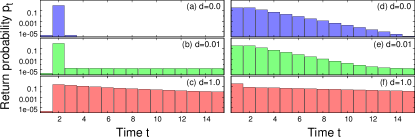
Figure 2: (Color online) Probability distributions of the first return time on a star graph of degree 6, for two different sets of random hopping amplitudes (left column, right column), and increasing decoherence rates (from top to bottom). The expected return time with no decoherence (top row) is $T_{0}=2$, with decoherence (middle and bottom row) it is $T_{0}=6$.

To understand how even an infinitesimal amount of decoherence can change the expected return time to $T_{0}=6$ from $T_{0}=2$, we explore the partial expected return time $T_{0}^{(L)}$, i.e., the expected return time after a finite number $L$ of timesteps. This quantity is defined by

$$T_{0}^{(L)} =\sum_{t=1}^{L}tp_{t}+(L+1)(1-\sum_{t=1}^{L}p_{t}),$$ (43)

where the DTQW is done for $L\in\mathbb{N}$ timesteps only, and if the walker does not return, it is assumed to return in timestep $L+1$. Although the expected return time $T_{0}$ does not depend on the hopping amplitudes $v_{j}$, the quantities $T_{0}^{(L)}$ do. To show the extent of this dependence, we sample the hopping amplitudes $v_{j}$ uniformly on the complex disk of unit radius and plot the median, the upper decile, and the lower decile of the distribution of the return times after $L$ timesteps $T_{0}^{(L)}$ in Fig. 3. As the number $L$ of observed timesteps increases, the range of the expected return times goes down, and the expected return times approach the asymptotic value.

Figure 3: (Color online) First return times after $L$ timesteps on a star graph of degree 6, as functions of decoherence rates $d$. The shaded areas are between the lower and upper decile, for $L=700$, $L=7000$, and $L=\infty$; the medians are shown with dashed lines.

IV.2 Breaking unitality: population transfer processes on complete graphs

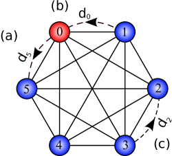
Figure 4: (Color online) A fully connected graph of $M=6$ nodes, on which a quantum walk is started from node 0. Each timestep consists of a coherent part, defined via a fixed random unitary operator (chosen uniformly from a Circular Unitary Ensemble), followed by an incoherent process that transfers population between two fixed sites, along a dashed line, as in Eq. (44). We consider three examples: where this population transfer delays the return (a), where it speeds up the return (b), and where it is neutral (c).

In a next set of examples we break unitality of a DTQW on a fully connected graph of $M$ nodes, in a controlled way. This is achieved using an asymmetric partial population transfer process that follows the coherent part of the timestep. If this population transfer is from a fixed “source” site to a fixed “target” site, it creates an accumulation of probability at the target site, and thus, is not unital. As a consequence, the expected return time will not be an integer, and will depend on the system parameters in a continuous way.

The incoherent partial population transfer from one fixed source site ($j+1$) to another fixed target site ($j$), with rate $d_{j}$, is defined via its Kraus operators $B_{0}^{(j)}$ and $B_{1}^{(j)}$, as

$$B_{0}^{(j)} =\sqrt{d_{j}}\,\big{|}\,{j}\,\big{\rangle}\big{\langle}\,(j+1)\,\text{mod}\,M\,\big{|};$$ (44a)

$$B_{1}^{(j)} =\mathbb{I}+(\sqrt{1-d_{j}}-1)|{j}\rangle\langle{j}|.$$ (44b)

The full timestep operator $\mathcal{S}$ of the DTQW of this Section consists of a unitary part, followed by partial population transfer,

$$\rho(t+1) =\mathcal{S}^{(j)}[\rho(t)]=\sum_{l=0,1}B_{l}^{(j)}U\rho(t)U^{\dagger}B_{l}^{(j)\dagger}$$ (45)

To study the effect of the asymmetric population transfer numerically, we used a fully connected graph of $M=6$ nodes, as shown in Fig. 4. There are 3 inequivalent ways of choosing the source and target nodes for the extra incoherent population transfer process, indicated by (a,b,c) in Fig. 4. In all of these cases, the population transfer breaks unitality, the expected return time $T_{0}$ can deviate from the number of nodes, $M$, and depends on the unitary operator $U$. To characterize this dependence, in each case we numerically determined the distribution of the expected return time $T_{0}$. We generated 2000 random instances of the operator $U$, picked uniformly from the set of unitary operators on the $M$-dimensional Hilbert space, using the circular unitary ensembleMezzadri (2007). For each value of the population transfer rate $d$, we calculated the median, and the upper and lower deciles of the distribution of the expected return time $T_{0}$.

Our numerical results, shown in Fig. 5, confirm that the asymmetric population transfer induces a spread of the expected return times. Moreover, depending on its direction, the population transfer can also change the average (median) of the return time. When the transfer is directed away from the initial state (i.e., the target site is $j=5$, case (a) in Fig. 4), the expected return times increase, as shown in Fig. 5(a). In the limit $d\to 1$, the expected return time diverges as $T_{0}\propto 1/(1-d)$, as it would in a classical walk. When the incoherent process drives the walker back towards the initial site ($j=0$, case (b) in Fig. 4), the average of the expected return time decreases as a function of the transfer rate, as shown in Fig. 5(b). In the limit $d\approx 1$, we find that the median is approximately half the number of sites, $M/2$, which matches the intuition that in this case, 2 out of $M$ sites correspond to successful return. Finally, for neutral population transfer ($j=2$, case (c) in Fig. 4), , as shown in Fig. 5(c), the expected return time $T_{0}$ acquires a spread due to the population transfer, but the median stays approximately independent of the population transfer rate.

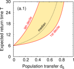
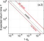
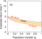
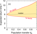
Figure 5: (Color online) The expected return time $T_{0}$ for a DTQW on a graph of 6 nodes, where a unitary operation is followed by asymmetric partial population tranfer towards the initial state. The unitary operator is picked at random from the circular unitary ensemble; thus, $T_{0}$ lies in the typical range shown by the shaded area, between the upper and lower decile (continuous lines), with the median also shown (dashed lines). If the population transfer is away from the origin, (a.1) and (a.2), the expected return times increase as a function of the population transfer rate. If it drives the walker back to the origin, (b), the expected return times decrease. For extra population transfer between two of the unobserved sites (c), the expected return time depends on the transfer rate.

IV.3 Breaking detailed balance but not unitality: Population transfer in a loop

Our final numerical example shows that asymmetric population transfer does not necessarily break unitality. We consider the population transfer to take place along a closed directed loop with uniform transfer rate $d$, as shown in Fig. 6, such that it induces a probability current. In that case, there is no detailed balance in the system, but the population transfer channel is unital, and so the expected return time does not deviate from the quantized value.

Figure 6: (Color online) A fully connected graph of 6 nodes, on which a quantum walk is started from node 0. Each timestep consists of a coherent part, defined via a Hamiltonian with random hopping amplitudes, followed by an incoherent process that transfers population in a loop along the dashed lines, as in Eqs. (46) and (47).

Each timestep consists of a unitary operation followed by the incoherent transfer,

$$\mathcal{S}[\rho]=\sum_{j=0}^{M}B_{j}U\rho U^{\dagger}B_{j}^{\dagger}.$$ (46)

The Kraus operators $B_{j}$ are defined as

$$B_{j} =\sqrt{d}|{j}\rangle\langle{j+1}|\quad\text{for }j=0,\ldots,M-2;$$ (47a)

$$B_{M-1} =\sqrt{d}|{M-1}\rangle\langle{0}|;$$ (47b)

$$B_{M} =\sqrt{1-d}\,\mathbb{I}.$$ (47c)

Since $\sum_{j=0}^{M}B_{j}B_{j}^{\dagger}=\mathbb{I}$, the whole timestep operator $\mathcal{S}$ is unital, and so the expected return time will be $M$, as confirmed by our numerics.

If the unitary operator $U$ is close to unity, it is worthwhile to look at the probability distribution of the return time $p_{t}$, since there is an interesting effect. $U=e^{-iH}$, where $H$ is a Hamiltonian with random hopping amplitudes uniformly distributed on the disk of radius $0.1$. In this case, almost no transitions happen during the coherent part of the timestep. Thus, for $d\approx 0$, we have $p_{1}\approx 1$, and the expected return time is $T_{0}=M$ only because of the exponential tail of the distribution. If the rate is $d\approx 1$, however, the walker is most likely taken on a round trip by the population transfer process, and so we obtain a peak in the distribution at $p_{M}\approx 1$. Fig. 7,

Figure 7: (Color online) Probability distributions of the first return time of a DTQW on a graph of degree 6, where a unitary operation is followed by an incoherent population transfer in a loop that includes all the sites. For the unitary part of the walk, we use $U=e^{-iH}$, with $H$ is a random Hermitian matrix with all matrix elements $\left|{H_{lm}}\right|<0.1$. Although the distributions are qualitatively different, their expectation values are all equal, $T_{0}=\sum_{t}tp_{t}=6$, because the walks are unital.

V Discussion

We proved that in iterated open quantum dynamical systems, unitality of the time evolution superoperator warrants that the expected return time is quantized. We introduced the concept of the relevant Hilbert space, which is spanned by the states of the system that can be reached from a given initial state, and proved that its dimension gives the expectation value of the first return time. Our work treats a broad class of physical systems on the same footing, including – as limiting cases – fully coherent iterated quantum dynamical systems (quantum walks), as well as classical Markov chains.

An immediate question raised by our work is: what about the expected return time in iterated quantum dynamical systems where the timestep superoperator is not unital? In the fully coherent case, this question does not arise, as the timestep superoperator can be constructed from a single unitary Kraus operator, and is thus always unital. In the fully classical limit, there is a well known answer to this question, given by the Kac lemmaKac (1947): the expected return time $T_{j}$ is the inverse of the maximum of the weight of the initial state $j$ in an equilibrium distribution (the maximum taken over all possible equilibria). Detailed analysis of our numerics, e.g., the data processed for Section IV.2, suggests that a statement analogous to the Kac lemma might hold for iterated open quantum dynamical systems. For an analytical treatment, however, more theoretical tools are needed, just as for the treatment of the recurrence to a more general initial condition, e.g., a subspace spanned by a set of initial statesBourgain et al. (2014).

As is often the case with classical concepts, the generalization of the notions of recurrence, and of the expected return time, from random walks to quantum walks is not unique. Besides the approach we take in this paper, there is an alternative route, an “ensemble approach”, useful to obtain estimations for efficiency of quantum protocols. This consists in letting the quantum walk run undisturbed and after a fixed time measure the position distribution of the walkerŠtefaňák et al. (2008), or its full quantum stateChandrashekar (2010b). The expected return time, defined in this way, does not necessarily take on an integer value even in the fully coherent case: it can exceed or stay below the dimension of the Hilbert spaceGrünbaum et al. (2013).

Recurrence is not only interesting for iterated open quantum dynamical systems, but for continous time processes as well, whose time evolution is prescribed by a quantum master equation. Here, to define a first return time, the time evolution is considered punctuated by measurements to detect the return of the walker. If these measurements are randomly timed, according to a Poisson process, the hitting times can become infinite even in the unitary caseVarbanov et al. (2008); no simple picture for the value of the return time has been yet found. The measurements can also be regularly timed: in this case, we obtain a continuous-time realization of the iterated open quantum dynamics, and our results considering the return time apply. In this latter case, it should be possible to cast the requirement of unitality, as well as the dimension of the relevant Hilbert space, in a simple formula for the Lindblad operators of the master equation. As an aside, there is a continuous-time generalization of the ensemble approach, with measurements that are either randomly distributed or regularly timedDarázs and Kiss (2010).

Our results give a concrete quantitative measure of the size of the part of the Hilbert space accessible from $|{\Psi}\rangle$. This could be a useful tool in the analysis of complex quantum networksFaccin et al. (2013, 2014). The expected return time $T_{\Psi}$, or, for a more detailed picture, the partial expected return times defined in Eq. (43), can be locally measured even with limited access to the full quantum network.

Appendix A Relevant Hilbert space

In this Section we prove some of the properties of the relevant Hilbert space used in the paper.

Take a Hilbert space $\mathcal{H}$, and take any superoperator $\mathcal{S}$, defined by its effect on density operators $\rho:\mathcal{H}\to\mathcal{H}$, via the Kraus operators $A_{j}$ as

$$\mathcal{S}[\rho]=\sum_{j=1}^{D}A_{j}\rho A_{j}^{\dagger}.$$ (48)

Take a pure state in the Hilbert space $|{\Psi}\rangle$. We denote by $\mathcal{M}$ the superoperator corresponding to filtering out the state $|{\Psi}\rangle$, i.e.,

$$\mathcal{M}[\rho]=(\mathbb{I}-|{\Psi}\rangle\langle{\Psi}|)\rho(\mathbb{I}-|{\Psi}\rangle\langle{\Psi}|).$$ (49)

We introduce a shorthand for (unnormalized) pure states obtainable from $|{\Psi}\rangle$ via the operators $A_{j}$. For each sequence $\underline{j}=(j_{1},\ldots,j_{t})$ of integers $j_{n}\in[1,D]$, we define

$$|{\underline{j}}\rangle =A_{j_{t}}\cdots A_{j_{2}}A_{j_{1}}|{\Psi}\rangle;$$ (50)

$$p_{\underline{j}} =\langle{\underline{j}}|{\underline{j}}\rangle.$$ (51)

The $t$th iterate of $|{\Psi}\rangle\langle{\Psi}|$ under $\mathcal{S}$ can be written with these states as

$$\mathcal{S}^{t}[|{\Psi}\rangle\langle{\Psi}|] =\sum_{j_{1}=1}^{D}\sum_{j_{2}=1}^{D}\ldots\sum_{j_{t}=1}^{D}|{\underline{j}}\rangle\langle{\underline{j}}|.$$ (52)

This is a probabilistic mixture of the pure states $|{\underline{j}}\rangle$ with weights $p_{\underline{j}}$.

Similarly, we use $|{\underline{j}}\rangle_{\text{cond}}$ to denote (unnormalized) pure states obtainable from $|{\Psi}\rangle$ via the operators $(\mathbb{I}-|{\Psi}\rangle\langle{\Psi}|)A_{j}$,

$$|{\underline{j}}\rangle_{\text{cond}} =(\mathbb{I}-|{\Psi}\rangle\langle{\Psi}|)A_{j_{t}}\cdots(\mathbb{I}-|{\Psi}\rangle\langle{\Psi}|)A_{j_{1}}|{\Psi}\rangle$$

$$=|{\underline{j}}\rangle+\sum_{n=2}^{t+1}c_{(j_{n},\ldots,j_{t})}(\underline{j})|{j_{n},\ldots,j_{t}}\rangle,$$ (53)

where the sequences $(j_{n},\ldots,j_{t})$ are obtained from the sequence $\underline{j}=(j_{1},\ldots,j_{t})$ by omitting the first $t-1$ elements (including the case $n=t+1$, where we obtain the empty sequence, for which according to Eq. (16), $|{\emptyset}\rangle=|{\Psi}\rangle$). The coefficients $c_{(j_{n},\ldots,j_{t})}(\underline{j})\in\mathbb{C}$ are complex numbers. The $t$th iterate of $|{\Psi}\rangle\langle{\Psi}|$ under $\mathcal{M}\mathcal{S}$ can be written using these states as

$$(\mathcal{M}\mathcal{S})^{t}[|{\Psi}\rangle\langle{\Psi}|] =\sum_{j_{1}=1}^{D}\sum_{j_{2}=1}^{D}\ldots\sum_{j_{t}=1}^{D}|{\underline{j}}\rangle_{\text{cond}}\langle{\underline{j}}|_{\text{cond}}.$$ (54)

The relevant Hilbert space $\mathcal{H}_{\Psi}(\mathcal{S},|{\Psi}\rangle)$ is the space spanned by the vectors $|{\underline{j}}\rangle$, for all admissible sequences $\underline{j}$ of any legth $t\in\mathbb{N}$. The projector to this subspace of $\mathcal{H}$ is the limit

$$\mathcal{\mathbb{I}}_{\Psi}(\mathcal{S},|{\Psi}\rangle) =\lim_{n\to\infty}\text{supp}(\sum_{t=0}^{n}\mathcal{S}^{n}[|{\Psi}\rangle\langle{\Psi}|]),$$ (55)

where $\text{supp}(\sigma)$ denotes the projector to the nonzero subspace (support) of a Hermitian operator $\sigma$.

It is clear by the construction of the set $\{|{\underline{j}}\rangle\}$ that the relevant Hilbert space is the smallest invariant subspace of $\mathcal{S}$ that contains $|{\Psi}\rangle$. It is an invariant subspace, since if $\sigma$ is a density operator in $\mathcal{H}_{\Psi}(\mathcal{S},|{\Psi}\rangle)$, then it can be decomposed as $\sigma=\sum_{\underline{j}}r_{\underline{j}}|{\underline{j}}\rangle\langle{\underline{j}}|$, and then $\mathcal{S}^{n}[\sigma]$ is also in $\mathcal{H}_{\Psi}(\mathcal{S},|{\Psi}\rangle)$, for any $n\in\mathbb{N}$. On the other hand, it contains $|{\Psi}\rangle$, and is the smallest such subspace, since it does not contain any state $|{\Phi}\rangle$ that is not reachable from $|{\Psi}\rangle$ by iterations of $\mathcal{S}$. Indeed, for such states $|{\Phi}\rangle$, we would have $\langle{\Phi}|\mathcal{S}^{t}[|{\Psi}\rangle\langle{\Psi}|]|{\Phi}\rangle=0$ for all $t\in\mathbb{N}$, and thus, they would be outside of $\mathcal{H}_{\Psi}(\mathcal{S},|{\Psi}\rangle)$.

We now show that the relevant Hilbert space is also spanned by the vectors $|{\underline{j}}\rangle_{\text{cond}}$, i.e., that

$$\mathcal{\mathbb{I}}_{\Psi}(\mathcal{S},|{\Psi}\rangle) =\mathcal{\mathbb{I}}_{\Psi}(\mathcal{M}\mathcal{S},|{\Psi}\rangle).$$ (56)

First, from the second line of Eq. (53), every vector ${|{\underline{j}}\rangle}_{\text{cond}}$ is expressed as a linear combination of vectors $|{\underline{j}}\rangle$, and so, $\mathcal{\mathbb{I}}_{\Psi}(\mathcal{M}\mathcal{S},|{\Psi}\rangle)\leq\mathcal{\mathbb{I}}_{\Psi}(\mathcal{S},|{\Psi}\rangle)$. On the other hand, every vector $|{\underline{j}}\rangle$ can be expressed as linear combination of $|{\underline{j}}\rangle_{\text{cond}}$ and of vectors $|{\underline{j}^{\prime}}\rangle_{\text{cond}}$, where the $\underline{j}^{\prime}$ are sequences shorter than $\underline{j}$. This can be shown using mathematical induction, started from sequences of length $t=1$, for which

$$|{(j_{j})}\rangle =|{(j_{1})}\rangle_{\text{cond}}+|{\Psi}\rangle\langle{\Psi}|{(j_{1})}\rangle,$$ (57)

and using Eq. (53) for the inductive step. Thus, $\mathcal{\mathbb{I}}_{\Psi}(\mathcal{S},|{\Psi}\rangle)\leq\mathcal{\mathbb{I}}_{\Psi}(\mathcal{M}\mathcal{S},|{\Psi}\rangle)$, and this, together with $\mathcal{\mathbb{I}}_{\Psi}(\mathcal{M}\mathcal{S},|{\Psi}\rangle)\leq\mathcal{\mathbb{I}}_{\Psi}(\mathcal{S},|{\Psi}\rangle)$ shown above, proves Eq. (56).

The results of this Appendix translate to DTQWs considered in the paper, and prove Eq. (16).

Appendix B Numerical methods for the expected return time

To study the expected return time numerically in more detail, we use the spectral decomposition of the conditional timestep operator $\mathcal{M}\mathcal{S}$. This method is applicable only if the matrix of $\mathcal{M}\mathcal{S}$ is diagonalizable, which is the generic case.

We first find all eigenstates $\chi_{n}$ of $\mathcal{M}\mathcal{S}$, for $n=1,\ldots,M^{2}$, with eigenvalues $\alpha_{n}\in\mathbb{C}$,

$$\forall n:\quad\mathcal{M}\mathcal{S}[\chi_{n}] =\alpha_{n}\chi_{n}.$$ (58)

The next step is to provide a decomposition of the initial state $|{\Psi}\rangle\langle{\Psi}|$ in terms of the eigenstates $\chi_{n}$,

$$|{\Psi}\rangle\langle{\Psi}| =\sum_{n}c_{n}\chi_{n}.$$ (59)

The coefficients $c_{n}\in\mathbb{C}$ in the decomposition can be found using the right eigenvectors of the matrix of $\mathcal{M}\mathcal{S}$. Using the above, we can write the expected return time as a geometric series, and obtain

$$T_{\Psi} =\text{Tr }{\tilde{\rho}}_{\text{cond}}=\sum_{n}\frac{c_{n}}{1-\alpha_{n}}\text{Tr }\chi_{n}.$$ (60)

To study convergence of the expected return time, we define the expected return time up until a finite number $L$ of timesteps, as

$$T_{\Psi}^{(L)} =\sum_{t=1}^{L}tp_{t}+(L+1)(1-\sum_{t=1}^{L}p_{t})=\sum_{t=0}^{L}q_{t},$$ (61)

efficiently calculated using the spectral decomposition as

$$T_{\Psi}^{(L)} =\text{Tr }\sum_{t=0}^{L}(\mathcal{M}\mathcal{S})^{t}[|{0}\rangle\langle{0}|]=\sum_{n}c_{n}\frac{\alpha_{n}^{L+1}-1}{\alpha_{n}-1}\text{Tr }\chi_{n}.$$ (62)

References

- Mack et al. (2014) G. Mack, S. Wallentowitz, and P. E. Toschek, Physics Reports 540, 1 (2014).
- Chandrashekar (2010a) C. Chandrashekar, Physical Review A 82, 052108 (2010a).
- Joos (2003) E. Joos, Decoherence and the Appearance of a Classical World in Quantum Theory, Physics and astronomy online library (Springer, 2003), ISBN 9783540003908, URL http://www.google.hu/books?id=6eTHcxeNxdUC.
- Lidar and Brun (2013) D. Lidar and T. Brun, Quantum Error Correction (Cambridge University Press, 2013), ISBN 9780521897877, URL http://books.google.hu/books?id=XV9sAAAAQBAJ.
- Perseguers et al. (2013) S. Perseguers, G. Lapeyre Jr, D. Cavalcanti, M. Lewenstein, and A. Acín, Reports on Progress in Physics 76, 096001 (2013).
- Venegas-Andraca (2012) S. Venegas-Andraca, Quantum Information Processing 11, 1015 (2012), ISSN 1570-0755, URL http://dx.doi.org/10.1007/s11128-012-0432-5.
- Schreiber et al. (2010) A. Schreiber, K. N. Cassemiro, V. Potoček, A. Gábris, P. J. Mosley, E. Andersson, I. Jex, and C. Silberhorn, Phys. Rev. Lett. 104, 050502 (2010), URL http://link.aps.org/doi/10.1103/PhysRevLett.104.050502.
- Karski et al. (2009) M. Karski, L. Förster, J.-M. Choi, A. Steffen, W. Alt, D. Meschede, and A. Widera, Science 325, 174 (2009), URL http://www.sciencemag.org/content/325/5937/174.full.
- Genske et al. (2013) M. Genske, W. Alt, A. Steffen, A. H. Werner, R. F. Werner, D. Meschede, and A. Alberti, Phys. Rev. Lett. 110, 190601 (2013), URL http://link.aps.org/doi/10.1103/PhysRevLett.110.190601.
- Sansoni et al. (2012) L. Sansoni, F. Sciarrino, G. Vallone, P. Mataloni, A. Crespi, R. Ramponi, and R. Osellame, Phys. Rev. Lett. 108, 010502 (2012), URL http://link.aps.org/doi/10.1103/PhysRevLett.108.010502.
- Broome et al. (2010) M. A. Broome, A. Fedrizzi, B. P. Lanyon, I. Kassal, A. Aspuru-Guzik, and A. G. White, Phys. Rev. Lett. 104, 153602 (2010), URL http://link.aps.org/doi/10.1103/PhysRevLett.104.153602.
- Zähringer et al. (2010) F. Zähringer, G. Kirchmair, R. Gerritsma, E. Solano, R. Blatt, and C. F. Roos, Phys. Rev. Lett. 104, 100503 (2010), URL http://link.aps.org/doi/10.1103/PhysRevLett.104.100503.
- Schreiber et al. (2011) A. Schreiber, K. N. Cassemiro, V. Potoček, A. Gábris, I. Jex, and C. Silberhorn, Phys. Rev. Lett. 106, 180403 (2011), URL http://link.aps.org/doi/10.1103/PhysRevLett.106.180403.
- Shenvi et al. (2003) N. Shenvi, J. Kempe, and K. B. Whaley, Phys. Rev. A 67, 052307 (2003), URL http://link.aps.org/doi/10.1103/PhysRevA.67.052307.
- Grover (1996) L. K. Grover, pp. 212–219 (1996), URL http://doi.acm.org/10.1145/237814.237866.
- Lovett et al. (2010) N. B. Lovett, S. Cooper, M. Everitt, M. Trevers, and V. Kendon, Phys. Rev. A 81, 042330 (2010), URL http://link.aps.org/doi/10.1103/PhysRevA.81.042330.
- Barreira (2005) L. Barreira, in IVth International Congress on Mathematical Physics (World Scientific, 2006) (Citeseer, 2005), vol. 415.
- Casati et al. (1999) G. Casati, G. Maspero, and D. L. Shepelyansky, Physical review letters 82, 524 (1999).
- Kemeny and Snell (1960) J. G. Kemeny and J. L. Snell, Finite Markov chains, vol. 356 (van Nostrand Princeton, NJ, 1960).
- Grünbaum et al. (2013) F. Grünbaum, L. Velazquez, A. Werner, and R. Werner, Communications in Mathematical Physics 320, 543 (2013), ISSN 0010-3616, URL http://dx.doi.org/10.1007/s00220-012-1645-2.
- Cirillo and Ticozzi (2014) G. I. Cirillo and F. Ticozzi, arXiv p. arXiv:1407.2566 (2014), URL http://arxiv.org/abs/1407.2566.
- Plenio and Huelga (2008) M. Plenio and S. Huelga, New J. Phys. (2008), URL http://iopscience.iop.org/1367-2630/10/11/113019.
- Rebentrost et al. (2009) P. Rebentrost, M. Mohseni, I. Kassal, S. Lloyd, and A. Aspuru-Guzik, New Journal of Physics 11, 033003 (2009), URL http://stacks.iop.org/1367-2630/11/i=3/a=033003.
- Attal et al. (2012) S. Attal, F. Petruccione, C. Sabot, and I. Sinayskiy, Journal of Statistical Physics 147, 832 (2012).
- Lardizabal and Souza (2014) C. F. Lardizabal and R. R. Souza, arXiv preprint arXiv:1402.0483 (2014).
- Kraus et al. (1983) K. Kraus, A. Böhm, and J. Dollard, States, Effects, and Operations Fundamental Notions of Quantum Theory, Lecture notes in physics (Springer, 1983), ISBN 9783540387251, URL http://books.google.hu/books?id=0l8dNQEACAAJ.
- Holbrook et al. (2003) J. Holbrook, D. Kribs, and R. Laflamme, Quantum Information Processing 2, 381 (2003), ISSN 1570-0755, URL http://dx.doi.org/10.1023/B%3AQINP.0000022737.53723.b4.
- Mezzadri (2007) F. Mezzadri, Notices of the AMS 54, 592 (2007).
- Kac (1947) M. Kac, Bulletin of the American Mathematical Society 53, 1002 (1947), URL http://projecteuclid.org/euclid.bams/1183511152.
- Bourgain et al. (2014) J. Bourgain, F. Grünbaum, L. Velázquez, and J. Wilkening, Communications in Mathematical Physics 329, 1031 (2014).
- Štefaňák et al. (2008) M. Štefaňák, I. Jex, and T. Kiss, Phys. Rev. Lett. 100, 020501 (2008), URL http://link.aps.org/doi/10.1103/PhysRevLett.100.020501.
- Chandrashekar (2010b) C. Chandrashekar, Central European Journal of Physics 8, 979 (2010b).
- Varbanov et al. (2008) M. Varbanov, H. Krovi, and T. A. Brun, Phys. Rev. A 78, 022324 (2008), URL http://link.aps.org/doi/10.1103/PhysRevA.78.022324.
- Darázs and Kiss (2010) Z. Darázs and T. Kiss, Phys. Rev. A 81, 062319 (2010), URL http://link.aps.org/doi/10.1103/PhysRevA.81.062319.
- Faccin et al. (2013) M. Faccin, T. Johnson, J. Biamonte, S. Kais, and P. Migdał, Phys. Rev. X 3, 041007 (2013), URL http://link.aps.org/doi/10.1103/PhysRevX.3.041007.
- Faccin et al. (2014) M. Faccin, P. Migdał, T. H. Johnson, V. Bergholm, and J. D. Biamonte, Phys. Rev. X 4, 041012 (2014), URL http://link.aps.org/doi/10.1103/PhysRevX.4.041012.