Information Sharing for Strong Neutrals on Social Networks - Exact Solutions for Consensus Times

Abstract

To analyze the nuances of the root concept of neutral in social networks, we focus on several related interpretations and suggest corresponding mathematical models for each of them from the family of information-sharing multi-agents network games known as Voter models and the Naming Games (NG). We solve the case of the strong neutrals known as the middle-roaders for global quantities such as expected times to consensus and local times. By using generating functions and treating the two extreme and middle opinions in this modification as a two balls, three urns version of the Voter model, we give closed-form expressions for the eigenvalues and eigenvectors of its Markov propagator. This modification of the two-opinions Naming Games is applicable to the roles and behaviour of neutrals in social forums or blogs, and represent a significant departure from the linguistic roots of the original NG.

1 Introduction

The Naming Games have been widely studied as a class of effective models for information sharing and opinion spread in social networks. Naming Games were first introduced in linguistics to model the convergence of social names or tags to a small or even single label [1], [2]. In the two opinions subclass (where the opinions or signals are denoted A and B) of the NG, the original model treats the neutrals as agents who have equal probability of signalling A or B. Thus, a speaker - listener pair chosen from the neutrals can either exit as a pair of purely A or B opinions agents. The neutral speaker has half probability of signalling A which is assumed to be received by the neutral listener with full fidelity who then, along with the speaker, becomes a purely A opinion agent. The same holds if the speaker signals the opinion B in which case, both speaker and listener switch from neutrals to purely B.

One of the previous point of departure from this original NG [3] is the listener-only version (LO-NG) analyzed in [4, 5] where the asymmetry between speaker and listener is changed significantly to empower the speaker in the sense that only the listener may switch to a different opinion type in a single time step. This was done at first to simplify the mathematical analysis of the NG but we emphasize another important aspect of the LO-NG, namely, that it more closely resemble social opinion dynamics and information sharing and less the original linguistic applications of the NG. Arguably, the agent that speaks is the more pro-active of the pair and seeks to convince the other of his opinions.

One aim in this paper is to analyze the nuances of the root concept of neutral in sociology settings where the above speaker - listener protocol have a range of asymmetry. We focus on three related interpretations of this concept, namely, (a) undecided as in binary elections or referendums to choose between two candidates A, B, (b) middle-roaders as in blogs or social forums on a single issue with FOR and AGAINST as the extreme opinions and possibly several intermediate opinions in between them, such as in the issue of gun control, and (c) erratic or flippant as in the listener only (LO-NG) versions of the two-opinions NG where the neutrals or AB agents speak the either opinion A or B with fixed probabilities.

Clearly, for category (a) the undecided neutrals (AB) will be more reluctant to speak than the decided agents (A or B), and this could be formalized by neutrals never chosen as speakers, only as listeners in the associated game. Otherwise, the interactions are the same as in the LO-NG.

In category (b) the middle-roaders in social forums say, are neither undecided nor flippant, but rather, are very likely to be staunch believers in their middle opinion or opinions (AB). This neutral behaviour can be formalized by what we call the M models, where the agents are divided into two disjoint classes, namely, (1) the extremers who hold the extreme opinions (A or B), convert other extremers to the opposite extreme opinion, and are converted to middle-roaders only by (single or multiple) exposure to the Devil’s Advocacy of middle-roaders given next, and (2) the middle-roader neutrals who do not interact with other neutrals, play the Devil’s Advocate when speaking to extremers ( eg, speak B to an A extremer or vice-versa), and when listening to an A(resp. B) extremer (once or multiple times) converts to the corresponding extreme opinion.

To put (b) into a wider context, we add for completeness another category (c) of middle-roader neutral behaviour who not only play the Devil’s Advocate when speaking to extremers, but when listening once or more times to an A (resp. B) extremer converts to the other extreme opinion B (resp. A).

The original LO-NG fits into this classification in the category (d) of neutrals (AB) who are flippant (randomly speak A or B) when speaking to both other neutrals and extremers, and when listening, converts to the extremer type corresponding to the signal received. In this same category, the extremers consistently speak their associated opinion, and when listening, convert to flippant neutrals upon receiving the opposite extreme opinion.

Finally, again for the sake of being more complete, we describe the category (e) which differs from the flippant neutral (LO-NG) only in the perverse conversion of a neutral (AB) to the opposite B (resp. A) extremer when receiving signal A (resp. B), irrespective of the speaker.

There are more categories and the complete list can be tabulated according to different versions of the two-body three urns models [6]. It seems that only the case (b) of middle-roaders can be solved exactly in the sense of diagonalizing the Markov transition matrix in closed form by using the generating functions method pioneered by Kac in his solution of the Ehrenfest Urn Problem [7]. Moreover, as shown below it is equivalent to the 3-Voter model.

In the rest of the paper, we will solve the M-models exactly to compute for large network1s, expected times to consensus. The results obtained here, without using the Diffusion Approximation or Fokker-Planck Master equation, but rather from direct probabilistic calculations at the level of random walks, agree with those in [8]. Moreover, our calculations below can be extended for all values of $M$ including the smallest case $M=3$ which is of special interest here because of its equivalence to the scenario (b) of middle-roaders neutrals in social dialog and blogs.

The $M$ models will be solved exactly to prove the result that starting from a population of $N/3$ agents in any one of the $M$ microstates including the $M-2$ neutral ones, the expected times to consensus, $\tau=O(N^{2})$ is much longer than the $O(NlogN)$ expected consensus times for the two-opinions LO-NG model in scenario (c) for erratic neutrals [4], [5].

2 Random Walk Model

We assume that the model is imposed on a complete graph. That is, every node is connected to every other node in the network. Let $n_{A}(m)$, $n_{B}(m)$, and $n_{C}(m)$ be the total number of nodes with opinions $A$, $B$, and $C$ respectively at discrete time step $m$. Since the total number of nodes in the graph, $N$, is constant, we can eliminate $n_{C}$ by taking $n_{C}(m)=N-n_{A}(m)-n_{B}(m)$. So, the probability distribution of macrostates $(n_{A}(m)=i,n_{B}(m)=j)$ at time step $m+1$ can be expressed in terms of information given at time $m$ as

$$\begin{split}a_{ij}^{(m+1)}=&p^{A}_{i-1j}a_{i-1j}^{(m)}+p^{A}_{i+1j}a_{i+1j}^{(m)}+p^{B}_{ij-1}a_{ij-1}^{(m)}+p^{B}_{ij+1}a_{ij+1}^{(m)}\\ &+p^{A-B}_{i-1j+1}a_{i-1j+1}^{(m)}+p^{A-B}_{i+1j-1}a_{i+1j-1}^{(m)}+r_{ij}a_{ij}^{(m)}.\end{split}$$ (1)

where

$$p^{A}_{ij}=q^{A}_{ij}=\frac{i(N-i-j)}{N(N-1)}$$

.

(2)

Each pair $(i,j)$ in equation (1) corresponds to a row of the Markov transition matrix, $\mathbf{T}$. The $m$ step propagator, $a_{ij}^{(m)}$, can be found by multiplying the initial distribution, $a_{ij}^{(0)}$, in vector form by the matrix $\mathbf{T}^{m}$. We will find the $m$ step propagator analytically by solving the spectral problem for the matrix $\mathbf{T}$.

3 The Spectral Problem

We extend the procedure found in ref. [6] for the 3 opinion Voter model on the complete graph. For eigenvalue $\lambda$ and corresponding eigenvector $\mathbf{v}$ with components $c_{ij}$, the spectral problem can be stated as

$$\begin{split}(\lambda-1)c_{ij}=&p^{A}_{i-1j}c_{i-1j}+p^{A}_{i+1j}c_{i+1j}+p^{B}_{ij-1}c_{ij-1}+p^{B}_{ij+1}c_{ij+1}+p^{A-B}_{i-1j+1}c_{i-1j+1}\\ &+p^{A-B}_{i+1j-1}c_{i+1j-1}-(2p_{ij}^{A}+2p_{ij}^{B}+2p_{ij}^{A-B})c_{ij}.\end{split}$$ (3)

To solve this, we introduce a generating function $G(x,y,z)$ defined by

$$G(x,y,z)=\sum_{i}\sum_{j}c_{ij}x^{i}y^{j}z^{N-i-j}.$$ (4)

The double sum is over all pairs $(i,j)\in\mathbb{Z}^{2}$, however we force the restriction that $c_{ij}=0$ when $i<0$, $j<0$ or $i+j>N$. These restrictions are equivalent to the requirement that there cannot be any negative powers in $G$. Using these, we express the spectral problem in equation (3) as a PDE in generating function form:

$$(x-z)^{2}G_{xz}+(y-z)^{2}G_{yz}+(x-y)^{2}G_{xy}=N(N-1)(\lambda-1)G.$$ (5)

To solve this, make the change of variables $u=x-y$, $v=y-z$, and $H(u,v,z)=G(x,y,z)$. Since this is a linear change of variables, we expect $H$ to have the same form as $G$, except with coefficients $b_{ij}$. The PDE for the spectral problem expressed in the new variables becomes

$$(u^{2}+2uv)H_{uz}-2uvH_{uv}+v^{2}H_{vz}-v^{2}H_{vv}-u^{2}H_{uu}=N(N-1)(\lambda-1)H.$$ (6)

This difference equation for the coefficients of $H$ can be written explicitly as

$$b_{ij}=\frac{(N-i-j+1)[(i-1)b_{i-1j}+(j-1)b_{ij-1}]}{N(N-1)(\lambda-1)+(i+j)(i+j-1)}.$$ (7)

To find the eigenvalues and eigenvectors, we only consider the cases in which equation (7) becomes singular for some $i=i^{\prime}$, $j=j^{\prime}$. This is possible only when the denominator in equation (7) is zero at this point. This shows that for $i^{\prime},j^{\prime}=0...N,\;i^{\prime}+j^{\prime}\leq N$, the set of eigenvalues is

$$\lambda_{i^{\prime}j^{\prime}}=1-\frac{(i^{\prime}+j^{\prime})(i^{\prime}+j^{\prime}-1)}{N(N-1)}.$$ (8)

If we take $\lambda=\lambda_{i^{\prime}j^{\prime}}$, then $b_{i^{\prime}j^{\prime}}$ can take any value. This is a reflection of the fact that any multiple of an eigenvector remains an eigenvector with the same eigenvalue. Without loss in generality, take $b_{i^{\prime}j^{\prime}}=1$. Now, for $i>i^{\prime}$, and $j>j^{\prime}$, equation (7) will never be singular and non-trivial. This will determine all of the values of $b_{ij}$ for any $\lambda_{i^{\prime}j^{\prime}}$.

Now we find $c_{ij}$ in terms of $b_{ij}$. We do this by expressing $H(u,v,z)$ in the original $(x,y,z)$ coordinates to obtain

$$c_{ij}=\sum_{k=i}^{i+j}\sum_{r=i+j-k}^{N-k}b_{kr}{k\choose i}{r\choose{i+j-k}}(-1)^{r-j}.$$ (9)

Thus we have found the solution to all eigenvalues and eigenvectors explicitly. Note that even though many eigenvalues are repeated, we find independent expressions for $b_{ij}$ for each repetition. This will give independent expressions for $c_{ij}$ for each independent $b_{ij}$ that had been computed above. This suggests that the matrix is diagonalizable, which allows us to express any distribution in the eigenbasis of $\mathbf{T}$.

4 Applications of the Spectral Solution

The solution to the spectral problem can be used to find many useful quantities related to the 3-Voter model. This is because we now know the $m$ step propagator exactly. We can express the probability of each macrostate as:

$$a_{ij}^{(m)}=\sum_{i^{\prime}j^{\prime}}d_{i^{\prime}j^{\prime}}\lambda_{i^{\prime}j^{\prime}}^{m}[\mathbf{v_{i^{\prime}j^{\prime}}}]_{ij}$$ (10)

Here, $[\mathbf{v_{i^{\prime}j^{\prime}}}]_{ij}$ is the $i,j$ component of the eigenvector corresponding to the eigenvalue $\lambda_{i^{\prime}j^{\prime}}$. The coefficients $d_{i^{\prime}j^{\prime}}$ represent the initial macrostate probability distribution, $a_{ij}^{(0)}$, expressed in the eigenbasis. That is, we gather the eigenvectors into a matrix $\mathbf{V}$ and solve $\mathbf{Vd}=\mathbf{a}^{(0)}$, where the components of $\mathbf{d}$ and $\mathbf{a}^{(0)}$ are $d_{i^{\prime}j^{\prime}}$ and $a_{ij}^{(0)}$ respectively. Since $\mathbf{T}$ is diagonalizable, $\mathbf{V}$ is invertible. This form is very convenient in the applications that follow.

4.1 Moments of Consensus Time

With the solution to the spectral problem known, we can find all moments of the consensus time exactly. The consensus time is the number of steps required until every node in the network has the same opinion state. Once the model has reached consensus, the system will never leave this state. In addition to the exact solution for the moments, we will also find an estimate of this quantity that is independent of the initial distribution that demonstrates the asymptotic dependence on $N$ and the moment, $p$.

Let $q_{m}$ be the probability that the system reaches consensus at time $m$. The $p^{th}$ moment of consensus time, $\tau$, as a function of the initial distribution can expressed as

$$E[\tau^{p}|\mathbf{d}=\mathbf{V^{-1}a}^{(0)}]=\sum_{m=0}^{\infty}q_{m}m^{p}.$$ (11)

We find the explicit form for $q_{m}$ to be

$$q_{m}=\frac{1}{N}[a_{1,0}^{(m-1)}+a_{0,1}^{(m-1)}+a_{N-1,0}^{(m-1)}+a_{N-1,1}^{(m-1)}+a_{0,N-1}^{(m-1)}+a_{1,N-1}^{(m-1)}].$$ (12)

Apply equation (10) to express this as

$$q_{m}=\frac{1}{N}\mathop{\sum_{i^{\prime}=0}^{N}\sum_{j^{\prime}=0}^{N-i^{\prime}}}_{i^{\prime}+j^{\prime}>1}d_{i^{\prime}j^{\prime}}\lambda_{i^{\prime}j^{\prime}}^{m-1}\{[\mathbf{v_{i^{\prime}j^{\prime}}}]_{1,0}+[\mathbf{v_{i^{\prime}j^{\prime}}}]_{0,1}\\ +[\mathbf{v_{i^{\prime}j^{\prime}}}]_{N-1,0}+[\mathbf{v_{i^{\prime}j^{\prime}}}]_{N-1,1}+[\mathbf{v_{i^{\prime}j^{\prime}}}]_{0,N-1}+[\mathbf{v_{i^{\prime}j^{\prime}}}]_{1,N-1}\}.$$ (13)

The sum is taken so that $i^{\prime}+j^{\prime}>1$ since the macrostate probabilities in equation (12) are independent of the other eigenvectors. That is, $d_{i^{\prime}j^{\prime}}=0$ for $i^{\prime}+j^{\prime}\leq 0$. This is because $\lambda_{i^{\prime}j^{\prime}}=1$ in these cases, which corresponds to the consensus points. To simplify notation, we define $s_{i^{\prime}j^{\prime}}$ to be

$$s_{i^{\prime}j^{\prime}}=d_{i^{\prime}j^{\prime}}\{[\mathbf{v_{i^{\prime}j^{\prime}}}]_{1,0}+[\mathbf{v_{i^{\prime}j^{\prime}}}]_{0,1}+[\mathbf{v_{i^{\prime}j^{\prime}}}]_{N-1,0}\\ +[\mathbf{v_{i^{\prime}j^{\prime}}}]_{N-1,1}+[\mathbf{v_{i^{\prime}j^{\prime}}}]_{0,N-1}+[\mathbf{v_{i^{\prime}j^{\prime}}}]_{1,N-1}\}.$$ (14)

Therefore, we express the moments of consensus time as

$$E[\tau^{p}|\mathbf{d}=\mathbf{V^{-1}a}^{(0)}]\sim\frac{1}{N}\mathop{\sum_{i^{\prime}=0}^{N}\sum_{j^{\prime}=0}^{N-i^{\prime}}}_{i^{\prime}+j^{\prime}>1}s_{i^{\prime}j^{\prime}}\frac{p!}{(1-\lambda_{i^{\prime}j^{\prime}})^{p+1}}.$$ (15)

This form for the moments of consensus time is a function of the initial distribution through the variable $s_{i^{\prime}j^{\prime}}$ defined in equation (14). The moments of consensus time usually vary by an $O(1)$ multiple when the initial distribution changes. Only when the system is initially near consensus will this multiple vary with $N$. If we assume this is not the case, we now seek to find the asymptotic dependence of the moments of consensus time on $N$ and the moment $p$.

Let $S^{(m)}$ be the probability that the system is not in consensus at time $m$. This is the sum over all probabilities $a_{ij}^{(m)}$ that do not correspond to consensus states. These probabilities are independent of the eigenvectors with eigenvalue $\lambda=1$ since consensus is a frozen state. Thus, $S^{(m)}=O(\lambda_{2}^{m})$, where $\lambda_{2}$ is the second largest eigenvalue. Therefore, the probability of entering consensus at time $m$ is given by $q_{m}=S^{(m-1)}-S^{(m)}=O\left(\lambda_{2}^{m}\frac{1-\lambda_{2}}{\lambda_{2}})\right)$. Now, we substitute this into equation (11) to obtain

$$E[\tau^{p}]=O(p!2^{-p}N^{2p})$$ (16)

.

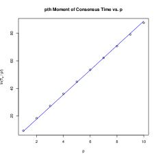
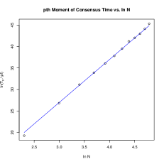
Figure 1: Monte carlo simulation results for the dependence on $p$ and $N$. In the top figure, we fix $N=120$ and take $p=1...10$. A line with slope $2\ln N-\ln 2$ corresponding to the theoretical prediction is also plotted. In the bottom figure, we fix $p=5$ and let $N=10,20,...,120$. The line is the best fit of the data that has slope $10$, which is the theoretical result we expect. These results show good correspondence between simulated and theoretical results.

This estimate is uniform over all initial distributions and considered a function of $p$ and $N$ only. This result shows that the expected time to consensus is $O(N^{2})$. We reinforce this result with two Monte Carlo simulations. In the first simulation, we fix $N=120$ and run the 3 opinion Voter model over 3000 runs. Let $T_{p}$ be the average of $\tau^{p}$ over all runs, which is the estimate of the $pth$ moment of consensus time. We predict that there is a linear relationship between $\ln(T_{p}/p!)$ and $p$, and that the slope of this line is about $2\ln N-\ln 2$. In the second simulation, we fix $p=5$ and let $N$ vary, we expect to find a linear relationship between $\ln(T_{p}/p!)$ and $\ln N$ with slope $2p=10$. Figure 1 shows the comparison between the simulated and predicted values.

4.2 Local Times

We can also apply the solution of the spectral problem to find all local times of the 3-Voter model. We define local times to be the expected time spent at each macrostate $(n_{A}=i,n_{B}=j)$ prior to consensus. We only consider macrostates that do not correspond to consensus states. Local times are stronger quantities than consensus times, because the sum of all local times will be equivalent to the expected time to consensus.

Let $M_{ij}(m)$ be the number of times steps spent at macrostate $(n_{A}=i,n_{B}=j)$ by time $m$. This is a monotonically increasing random walk, where

$$M_{ij}(m+1)=M_{ij}(m)+\Delta M_{ij}(m).$$ (17)

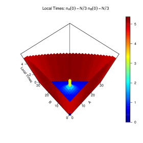
Figure 2: Local times of the 3-Voter model in the case when $n_{A}(0)=N/3$, $n_{B}(0)=N/3$ and $N=30$. The model spends most of the time at the boundary, in which the model is reduced to the 2-Voter model.

At time $m$, the randomness of the walk is exhibited in $\Delta M_{ij}(m)$, which can take values in $\{0,1\}$. If the model is in macrostate $(n_{A}=i,n_{B}=j)$ at time $m+1$, then $\Delta M_{ij}(m)=1$. This occurs with probability $a_{ij}^{(m+1)}$. So, we have that $E[\Delta M_{ij}(m)]=a_{ij}^{(m+1)}$. With this, we can find the local time for macrostate $(n_{A}=i,n_{B}=j)$:

$$E[M_{ij}(\infty)-M_{ij}(0)]=\sum_{m=0}^{\infty}a_{ij}^{(m)}$$ (18)

Utilize equation (10) to obtain the exact expression for local times:

$$E[M_{ij}(\infty)]=N(N-1)\mathop{\sum_{i^{\prime}=0}^{N}\sum_{j^{\prime}=0}^{N-i^{\prime}}}_{i^{\prime}+j^{\prime}>1}\frac{d_{i^{\prime}j^{\prime}}[\mathbf{v_{i^{\prime}j^{\prime}}}]_{ij}}{(i^{\prime}+j^{\prime})(i^{\prime}+j^{\prime}-1)}.$$ (19)

We write the sum such that $i^{\prime}+j^{\prime}>1$ because we do not consider consensus states when computing local times. The macrostates we consider are independent of the eigenvalue $\lambda=1$, which correspond to $i^{\prime}+j^{\prime}=0$ or $i^{\prime}+j^{\prime}=1$. Figure 2 shows the local time for the 3-Voter model when $n_{A}(0)=N/3$, $n_{B}(0)=N/3$ and $N=30$.

5 Conclusion

We have found concrete mathematical correlates for three different interpretations of neutral in sociology and politics. All three mathematical models belong to the generalized Listener Only NG and can therefore be systematically analyzed for key statistical quantities such as expected times to multi-consensus as in this paper.

In general, the deterministic drift in the coarse-grained or random walk models corresponding to each of these three families of NG-like models plays a key role. With increasing slow-time drift towards points of consensus, the expected times to consensus are decreased for most initial states. Meanwhile, such an increased drift against the committed minority consensus (near the consensus point of the position without committed fraction) generally predicts a relatively larger tipping fraction of committed minority agents, as a direct mathematical consequence of the saddle-node bifurcation on the slow-time manifold in phase-space.

Specifically, we have given exact solutions for expected times to multi-consensus $\tau$ in the M-models for all values of $M>2$ - $\tau\approx O(N^{2})$. Compared to the corresponding times for the original LO-NG on two opinions in scenario (c) which is $O(N\ln N)$, the strong neutrals (middle-roaders) have, as predicted in an early section, increased the expected times to multi-consensus for large networks. For a complete list of cases of the 2-Voter models solvable by this generating function approach, we refer the reader to a prior paper [6].

Another conclusion that we can draw from the drift-less nature of the $M$ models is that there are no positive (nonzero) tipping points for committed minority agents in any opinion type - even a very small number of committed agents of any type will tilt the $M$ game dynamics towards faster consensus of that opinion. This can be viewed as a disadvantage of the $M$ models for scenario (b) because bloggers in a social forum of different neutral positions are unlikely to be bowled over by extremely small numbers of committed leader-agents. In future work, we will attempt to fix this defect.

References

References

- [1] A. Baronchelli, M. Felici, V. Loreto, E. Caglioti, L. Steels, Sharp transition towards shared vocabularies in multi-agent systems.
- [2] A. Baronchelli, V. Loreto, L. Steels, In-depth analysis of the naming game dynamics: the homogeneous mixing case.
- [3] A. Baronchelli, Role of feedback and broadcasting in the naming game. 83 (2011) 046103.
- [4] J. Xie, S. Sreenivasan, G. Korniss, W. Zhang, C. Lim, B. K. Szymanski, Social consensus through the influence of committed minorities, Phys. Rev. E.
- [5] W. Zhang, C. Lim, S. Sreenivasan, J. Xie, B. Szymanski, G. Korniss, Social influencing and associated random walk models: Asymptotic consensus times on the complete graph, Chaos 21 (2011) 025115.
- [6] W. Pickering, C. Lim, Exact solution to the voter model by spectral analysis, submitted 2014.
- [7] P. Ehrenfest, T. Ehrenfest, Über zwei bekannte einwände gegen das boltzmannsche h- theorem, Physik Z. 8 (1907) 311.
- [8] M. Starnini, A. Baronchelli, R. Pastor-Sartorras, Ordering dynamics of the multi-state voter model.