Optimum reduction of the dynamo threshold by a ferromagnetic layer located in the flow

Abstract

We consider a fluid dynamo model generated by the flow on both sides of a moving layer. The magnetic permeability of the layer is larger than that of the flow. We show that there exists an optimum value of magnetic permeability for which the critical magnetic Reynolds number for dynamo onset is smaller than for a nonmagnetic material and also smaller than for a layer of infinite magnetic permeability. We present a mechanism that provides an explanation for recent experimental results. A similar effect occurs when the electrical conductivity of the layer is large.

Several properties of hydrodynamic instabilities are highly sensitive to the boundary conditions of the system. This is generically the case for the instability threshold. Changing the boundary conditions modifies the form of the unstable mode which results in a change in the efficiency of the processes responsible for the instability. This, in turn, modifies the values of the system parameters that are necessary to reach the instability threshold. In the canonical example of Rayleigh-Bénard convection in a layer of infinite horizontal extension with fixed temperature at the top and bottom boundaries, the threshold, measured by the Rayleigh number, differs by a factor close to three depending if the boundary conditions for the velocity field are no-slip or stress-free chandra .

For the dynamo instability, the boundary conditions for the magnetic field are also crucial. For astrophysical applications, the physical properties of the external or internal boundaries are sometimes so poorly constrained that models are free to investigate boundaries with completely different properties. In experiments, dynamos are difficult to observe because they are generated by turbulent flows of liquid metals driven at very large velocities. Experiments are often operated at the limit of the achievable parameters. Therefore even a small reduction of the dynamo threshold is always welcome while an increase can easily turn a successful experiment into a failure.

The Von Karman Sodium experiment (VKS) P1 consists of a swirling flow of liquid sodium that is driven by the counter-rotation of two disks fitted with blades. A strong shear is present in the mid-plane between the disks. This shear converts poloidal to toroidal magnetic field through the $\omega$-effect. Moreover, the flow is helical close to the disks, which generates an $\alpha$-effect that can convert toroidal to poloidal magnetic field gafd . A dynamo is only observed when the propellers are made of soft iron which has large magnetic permeability; thus the boundary conditions are also of great importance. The effects of boundary conditions on the VKS dynamo have been investigated in several studies. The boundaries of the container were initially considered ravelet . Experimentally, the nature of these boundaries was observed to be far less important that the nature of the disks. The first attempt to model the disks was to assume that their large magnetic permeability constrains the field to be purely normal to the propeller boundaries gafd , nore , gissinger . A second idea relies on treating the effect of the blades as an inhomogeneous magnetic permeability in the azimuthal direction. Inhomogeneities of the electrical conductivity are known to be able to generate a dynamo provided that an $\omega$-effect acts close to the boundary wicht . A similar idea was put forward to explain numerical simulations of the VKS experiment guisecke . The mechanism has been identified and calculated analytically in model geometries gallet1 , gallet2 . From these calculations, the effect of inhomogeneities appears as an additional induction mechanism that converts toroidal to poloidal field. However, the effect is not very efficient and very large magnetic Reynolds numbers are necessary to generate a dynamo. It has also been suggested that the motion of the soft iron disk leads to an increase in the $\omega$-effect and that the effect depends on the magnetic Reynolds number based on the disk properties verhille .

Assuming that a boundary can be modeled as a medium of large magnetic permeability, one can classify the possible effects into two groups. (i) The change in boundary conditions lowers the onset of a mode that would be a dynamo at higher onset with nonmagnetic material. (ii) The boundary provides a new amplification mechanism that is responsible for the dynamo action and without which a similar dynamo would not exist. In the mechanisms reported so far, the effect of the blades (inhomogenous magnetic permeability) belongs to group (ii) while the other effects are of group (i).

We present here another mechanism that belongs to group (i). We focus on a single disk and consider the structure of the magnetic field on both sides of the disk. Indeed, the symmetries of the flow constrain several properties of the induction process. For instance, shears of opposite signs are located on either side of the propeller. Then, we show that a large but finite value of the magnetic permeability of the disk results in a decrease of the dynamo threshold compared to the case of a nonmagnetic or ideal ferromagnetic material.

A simple geometrical configuration is considered to model the disk and the flow. The configuration is presented first, along with the methods used to solve the problem. Numerical results are then presented and extended to the case of a change in the electrical conductivity. We finish with an explanation of the increased efficiency of the dynamo for certain optimal values of the disk physical properties.

Presentation of the calculation

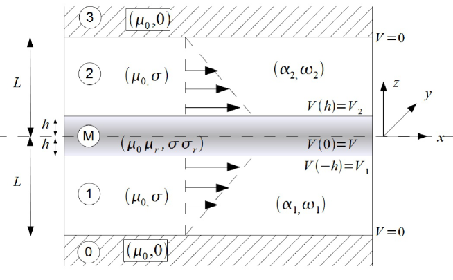
Figure 1: Sketch of the model. A layer $(M)$ moves at constant velocity $V$ and is located in-between two medium $(1)$ and $(2)$ in which $\omega$ and $\alpha$ effects are present. The outer medium $(0)$ and $(3)$ are insulating.

To simplify the problem, we consider a cartesian geometry as sketched in fig. 1. The $x,y$ and $z$ coordinates correspond to the $\theta,r$ and $z$ coordinates in cylindrical geometry. A fluid of magnetic permeability $\mu_{0}$ and electrical conductivity $\sigma$ is located between $z=-L$ and $z=-h$ and between $z=h$ and $z=L$. A third layer of magnetic permeability $\mu_{0}\mu_{r}$ and electrical conductivity $\sigma\sigma_{r}$ is located between these two layers. The outer medium $|z|\geq L$ is insulating and non-magnetic, as is a vacuum.

The induction processes in the fluid layers are modeled using the equations of mean-field magnetohydrodynamics. We thus solve

$$\frac{\partial{\bf B}}{\partial t}=\nabla\times\left({\bf v}\times{\bf B}+\alpha{\bf B}\right)+\eta\nabla^{2}{\bf B}\,,$$ (1)

where $\bf v$ is the large-scale velocity field and $\alpha$ is the tensor of the $\alpha-$effect. This tensor describes the effect of small-scale velocity structures on the large-scale magnetic field moffatt . In the first (resp. second) layer, two induction processes are considered: a shear of strength $\omega_{1}$ (resp. $\omega_{2}$) associated to a velocity $v^{(1)}_{x}=\omega_{1}(z+L)$ (resp. $v^{(2)}_{x}=\omega_{2}(z-L)$) in the $x$ direction and an $\alpha$-effect $\alpha^{(1)}$ (resp. $\alpha^{(2)}$). The shear converts magnetic field in the $z$-direction into a field in the $x$-direction. The $\alpha$-effect converts magnetic field along $x$ in a current along $x$, i.e. $\alpha^{(u)}_{i,j}=\alpha_{u}\delta_{i,x}\delta_{j,x}$. The mid-layer translates at a uniform speed $V$. We use $L$ and $L^{2}\mu_{0}\sigma$ as the units of length and time, respectively and we define the following dimensionless numbers $R_{\omega_{i}}=\mu_{0}\sigma\omega_{i}L^{2}$, $R_{\alpha_{i}}=\mu_{0}\sigma\alpha_{i}L$, for $i=1,2$ and $R_{V}=\mu_{0}\sigma VL$.

To solve equation 1, we seek for modes of the form ${\bf b}(z)\exp{i(pt+ky)}$ where $p$ is the growth rate and $k$ the wave-vector in the $y$-direction. Our restriction to solutions independent of the $x$-coordinate corresponds to axisymmetric large-scale fields in the cylindrical geometry of the VKS experiment. Using the divergence-free property of the magnetic field, we can eliminate $b_{y}$ from the problem and we have to solve the following coupled equations for the $x$ and $z$ components. In layer $j$, for $j=1,2$, equation 1 reads

$$\left(p+k^{2}\right)b_{x}^{(j)}-\partial_{zz}b_{x}^{(j)}-R_{\omega_{j}}b_{z}^{(j)}=0\,,$$ (2)

$$\left(p+k^{2}\right)b_{z}^{(j)}-\partial_{zz}b_{z}^{(j)}+R_{\alpha_{j}}ikb_{x}^{(j)}=0\,.$$ (3)

In the mid-layer $M$, we solve a diffusion equation with a relative dimensionless diffusivity $\eta_{r}=1/(\sigma_{r}\mu_{r})$,

$$\left(p/\eta_{r}+k^{2}\right)\textbf{b}^{(M)}=\partial_{zz}\textbf{b}^{(M)}$$ (4)

while in the outer insulating medium, we solve the equation $\nabla\times\bf B=0$. Using the divergence-free condition, this reduces to

$$\partial_{zz}\textbf{b}_{z}^{(j)}=k^{2}\textbf{b}_{z}^{(j)}$$ (5)

and $\partial_{y}\textbf{b}_{x}^{(j)}=\partial_{z}\textbf{b}_{x}^{(j)}=0$, for $j=0,3$. These equations must be supplemented with boundary conditions. Using continuity of the normal component of the magnetic field, of the tangential component of ${\bf b}/\mu$, and of the tangential component of the electric field, we obtain four relations at each interface between medium $i$ and $j$

$$b_{z}^{(i)}=b_{z}^{(j)},\quad\quad\frac{b_{x}^{(i)}}{\mu_{r}^{(i)}}=\frac{b_{x}^{(j)}}{\mu_{r}^{(j)}},\quad\quad\frac{\partial_{z}b_{z}^{(i)}}{\mu_{r}^{(i)}}=\frac{\partial_{z}b_{z}^{(i)}}{\mu_{r}^{(j)}},\quad\quad E_{y}^{(i)}=E_{y}^{(j)}$$ (6)

where

$$E_{y}^{(i)}=u_{x}^{(i)}b_{z}^{(i)}+\frac{1}{\mu_{r}^{(i)}\sigma_{r}^{(i)}}\partial_{z}b_{x}^{(i)}.$$ (7)

The eigenvalues $p$ of this linear problem are found by seeking solutions that decrease to zero as $|z|$ tends to infinity. The solutions in the outer medium involve two unknown constants and using the boundary conditions, these constants can be eliminated to obtain two new boundary conditions for the field in medium $1$ (resp. $2$) at $z=-1$ (resp. $z=1$). These new boundary conditions do not involve the value of the field in the outer medium.

We now have to calculate the possible values of $p$ and the associated spatial structure of the magnetic field eigenmodes. We have solved this problem with two different and standard methods. The first method is to solve analytically the equations in each layer. Each solution in layer $1$, $M$ and $2$ involves four unknown constants as the problem can be written as one fourth-order differential equation for a single function (either $b_{x}$ or $b_{z}$) in medium $1$ or $2$, and as two separated second-order equations for $b_{x}$ and $b_{z}$ in medium $M$. The twelve boundary conditions form a linear set of equations for the unknown constants. The existence of non-zero solutions requires the cancellation of the determinant of this set of equations. The problem has thus been turned into that of finding zeros of a determinant. This equation selects the possible values of $p$.

The second method consists in solving the equations numerically using a spatial discretization of $N$ gridpoints in each layer. The values of the two components of the field at these $3N$ gridpoints form a vector of size $6N$. We obtain a set of $6N$ linear equations by writing the two equations (Eq. (2) and (3) or the $x$ and $z$ component of Eq. (4)) evaluated at the $3N$ gridpoints and by taking into account the boundary conditions. Eigenvalues of the associated matrix are possible growth rates $p$.

Each of the two methods has its own advantages and drawbacks. For the first method, one must find zeros of a complicated function. This defines an implicit expression of $p$ as a function of the problem parameters. Standard methods require initial guesses for the zeros and inaccurate guesses can result in solutions that are not the most unstable. In contrast, with the second method, approximations of $6N$ eigenvalues are found but these are only approximations and one needs to check the convergence of the numerical results when $N$ is increased. For the results presented below, we have checked that both methods give the same results provided $N$ is large enough. Typically, with $N$ of order $100$, the difference between the two methods is smaller than $0.05\%$ for the onset of the first eigenmodes.

The problem involves a large number of parameters. In dimensionless form there are nine parameters, namely $k$, $h$, $\sigma$, $\mu$, $R_{\omega_{1}}$, $R\alpha_{1}$, $R_{\omega_{2}}$, $R\alpha_{2}$, $R_{V}$. Obviously one cannot consider performing a parametric study for such a general problem. What we have done is to highlight one particular effect observable in this configuration: the decrease of the dynamo threshold when the mid-layer has a large but finite magnetic permeability (or electrical conductivity). We have checked that the effect is robust by changing drastically some hypotheses, aspect ratio or symmetry of the flow.

Results

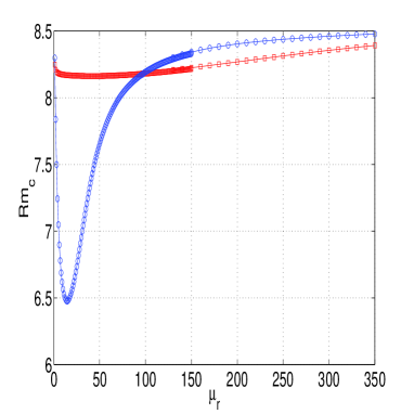
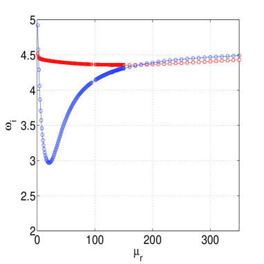
Figure 2: Left: Onset of the two eigenmodes with largest growth rates as a function of the magnetic permeability $\mu_{r}$ of the mid-layer; for a symmetric configuration $R_{\omega_{1}}=R\alpha_{1}=-R_{\omega_{2}}=-R\alpha_{2}=R_{V}=$Rm and $\sigma_{r}=1$, $h=1/20$, $k=1$. Right: Frequencies of the two eigenmodes with largest growth rate. Blue circles (resp. red squares) are the even (resp. odd) mode.

We first present a situation in which the induction mechanisms are of same intensity but have opposite signs in the two layers. We thus choose $R_{\omega_{1}}=R\alpha_{1}=-R_{\omega_{2}}=-R\alpha_{2}=$Rm. We consider that the mid-layer is moving at the same speed as the flow at $|z|=h$, thus $R_{V}=$Rm. The onsets Rm_c of the two most unstable modes are presented in fig. 2 for $k=1$ and $h=1/20$. Both curves display a minimum at a finite value of $\mu_{r}$. For one of the modes, the onset reduction compared to $\mu_{r}=1$ is of the order of $25\%$. For the other mode, the reduction is very small, of the order of $1\%$. We also note that both modes are oscillatory which amounts to propagation in the $y$-direction. This is expected since the problem is not invariant under $y\rightarrow-y$ (as the $\alpha$ coefficients are pseudo-scalars).

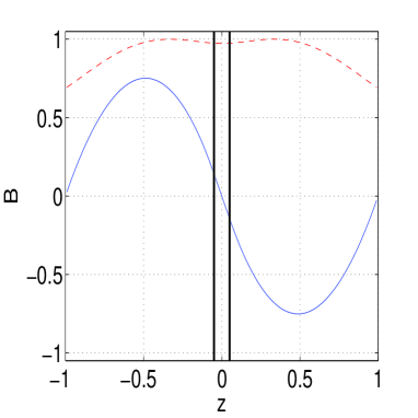
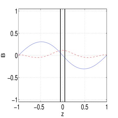
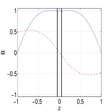
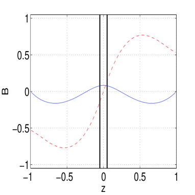
Figure 3: Eigenmodes at their onset for a symmetric configuration and $\mu_{r}=1$, $\sigma_{r}=1$, top: most unstable mode Rm$=8.25$. Bottom: second most unstable mode Rm$=8.3$. Real part (resp. imaginary part) are displayed on the left (resp. right). The $x$ (toroidal) component is the continuous (blue) curve. The $z$ (poloidal) component is the dashed (red) curve.

The shape of the eigenmodes is presented in fig. 3, 4, 5. The two modes have opposite symmetries. The continuous (blue) curve is the $x$ (toroidal) component and the dotted (red) curve is the $y$ (poloidal) component. Since the problem is invariant under $z-$reflection, the eigenmodes are either odd or even under this transformation. Consequently, the components $b_{z}$ and $b_{x}$ are of opposite parities. For $\mu_{r}=1$, the even mode is the most unstable one but both modes have comparable thresholds. This is also the case for very large $\mu_{r}$. As expected in the limit of high permeability, the field is nearly normal to the mid-layer boundary at $|z|=h$. For $\mu_{r}=14.5$, the odd mode is the most unstable and is responsible for the decrease in the value of Rm at onset. We observe that even though the $z$ (poloidal) component changes sign in the mid-layer, this is achieved over the short width of the mid-layer, so that the field is large everywhere in the fluid even close to the mid-layer.

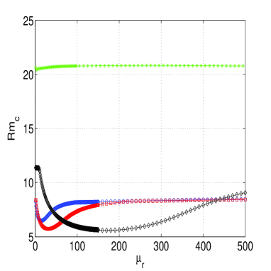
Figure 6: Onset of the most unstable eigenmode as a function of the magnetic permeability $\mu_{r}$ of the mid-layer; for a symmetric configuration $R_{\omega_{1}}=R\alpha_{1}=-R_{\omega_{2}}=-R\alpha_{2}=R_{V}=$Rm, $\sigma_{r}=1$, $h=1/20$ and (green star): $k=5$, (blue circle): $k=1$, (red square): $k=0.5$, (black diamond): $k=0.1$.

We have investigated how the transverse wavelength affects the reduction of the onset. The onset of the most unstable mode is presented as a function of $\mu_{r}$ for different values of $k$ in fig. 6. For large $k$, the reduction of onset is very small. It increases when $k$ is decreased. For instance, in the case $k=0.1$, the onset is Rm${}_{c}=11.3$ for $\mu_{r}=1$ and at very large $\mu_{r}$, is around Rm${}_{c}\simeq 11$. The onset is decreased to Rm${}_{c}=5.6$ (a reduction around $50\%$) at $\mu_{r}=170$.

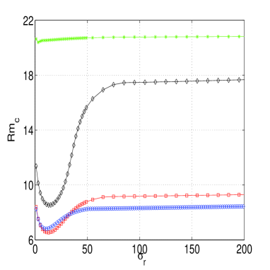
Figure 7: Onset of the most unstable eigenmode as a function of the electrical conductivity $\sigma_{r}$ of the mid-layer; for a symmetric configuration $R_{\omega_{1}}=R\alpha_{1}=-R_{\omega_{2}}=-R\alpha_{2}=R_{V}=$Rm, $\mu_{r}=1$, $h=1/20$ and (green star): $k=5$, (blue circle): $k=1$, (red square): $k=0.5$, (black diamond): $k=0.1$.

We have performed similar studies in the case $\mu_{r}=1$ and varying the electrical conductivity of the mid-layer $\sigma_{r}$. Results qualitatively similar to the case of varying $\mu_{r}$ are obtained for the onset reduction, as displayed in fig. 7. However, the values of Rm_c are quantitatively different from what is presented in fig. 2 so that there is no symmetry in exchange of magnetic permeability and electrical conductivity, i.e. Rm${}_{c}(\mu_{r},\sigma_{r})\neq$ Rm${}_{c}(\sigma_{r},\mu_{r})$, as expected from equations 6 and 7.

The shape of the eigenmodes (not presented here) displays the following properties. At large electrical conductivity, the field is nearly tangent to the mid-layer boundary, as expected. At intermediate conductivity, the smallest value of onset is achieved by a field whose $x$ (toroidal) component changes sign over a short length scale in the mid-layer so that this component is large in the fluid even close to the mid-layer. We summarize the effect of an increase of conductivity by noting that the reduction of the value of Rm_c is qualitatively similar to that obtained for an increase of the magnetic permeability, but the roles of the poloidal and toroidal components are exchanged.

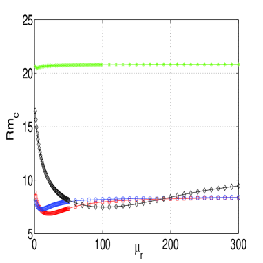
Figure 8: Onset of the most unstable eigenmode as a function of the magnetic permeability $\mu_{r}$ of the mid-layer; for an asymmetric configuration $R_{\omega_{1}}=R\alpha_{1}=-R_{\omega_{2}}=R_{V}=$Rm, $R\alpha_{2}=0$, $h=1/20$, $\sigma_{r}=1$ and (blue circle): $k=1$, (red square): $k=0.5$, (black diamond): $k=0.1$. An $\omega$ and an $\alpha$-effect are operating in layer $1$ while only $\omega$-effect is considered in layer $2$.

In the VKS experiment, the role of the mid-layer is played by the disks. These disks are fitted on one side with blades. The two sides of the disks are thus different. If shear is present close to both sides, helical vortices are expected to be more intense close to the blades. A natural question is whether the effect that we have identified in the case of a symmetric configuration (with induction effects of opposite intensities on both sides of the disks) remains efficient if the flow is modified. We thus consider the case in which an $\alpha$-effect only operates in one layer (layer $1$) and is zero in the other layer. We show the value of the threshold of the most unstable mode in fig. 8 for different values of $k$. We observe that a reduction of the threshold also takes place in the asymmetric configuration. As in the symmetric case, the effect is more intense when the wavelength in the transverse direction is increased.

For the spatial structure of the modes, the system being asymmetric, the modes are neither odd nor even functions of $z$. Nevertheless, some properties of the symmetric configuration are still verified: compared to the case $\mu_{r}=1$ or large $\mu_{r}$, the $z$ (poloidal) component of the most unstable mode displays a strong gradient in the mid-layer for intermediate $\mu_{r}$. Consequently, the field is large everywhere in layer $1$ where both induction effects are present.

It has been suggested that the disks in the VKS experiment are responsible for an increased $\omega$-effect, the intensity of which increases with the magnetic Reynolds number based on the disk magnetic permeability, electrical conductivity, speed and size, i.e. $\mu_{r}\sigma_{r}R_{V}$ verhille . To check whether a similar description could explain the onset reduction that we have identified in this work, we have varied $\mu_{r}$ keeping fixed the value $\mu_{r}\sigma_{r}=1$. A decrease in onset is observed at intermediate values of $\mu_{r}$ which rules out an effect controlled by the value of the magnetic Reynolds number of the layer.

Finally, since the disk electrical conductivity is different from that of the fluid in the liquid sodium experiment, we have changed the value of $\sigma_{r}$ and investigated how Rm_c depends on $\mu_{r}$. In the cases that we considered ($\sigma_{r}$ equals to $0.1$, $0.2$, $1$ and $5$), we always observe a decrease of the critical magnetic Reynolds number for a value of $\mu_{r}$ that slightly decreases with $\sigma_{r}$ (from $17.8$ for $\sigma_{r}=0.1$ to $12.5$ for $\sigma_{r}=5$).

Description of the mechanism and conclusion

We now describe the physical mechanism responsible for the decrease in onset. For simplicity we consider the symmetric case. The $\alpha$ and $\omega$ effects on either side of the layer have opposite signs. This implies that the poloidal and toroidal components have the same sign on one side and opposite signs on the other side. Then, even though the $\alpha$ and $\omega$ effects change sign, in both domains the induction mechanisms act to amplify the magnetic field. As a consequence, one of the components vanishes at the center of the mid-layer and changes sign. In other words, from the point of views of symmetries, the magnetic modes must be either odd or even with respect to reflection at the plane $z=0$, which is what we have just obtained from the discussion of the properties of the induction processes.

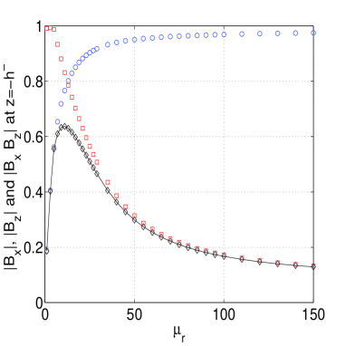
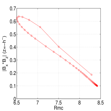
Figure 9: Left: Value of $|B_{x}|$ (red square), $|B_{z}|$ (blue circle) and their product (black diamond) as a function of $\mu_{r}$ at the onset of the odd mode at $z=-h$ in the fluid. Same parameter values as in fig. 2. The fields are normalized by the maximum of $|B_{x}|$ and $|B_{z}|$ in the fluid. Right: $|B_{x}B_{z}|$ at $z=-h$ as a function of Rm_c (same datas as left figure).

For $\mu_{r}=1$, when one of the components changes sign in the mid-layer, it is small close to the mid-layer. There, the intensity of the induction mechanisms is smaller than if the magnetic field were large. In the limit of infinite magnetic permeability, the tangential component vanishes at the mid-layer boundary and the field is purely normal. Just as for $\mu_{r}=1$, because the tangential component vanishes at the mid-layer, the efficiency of one of the induction processes (the $\alpha$ effect) is also small near the mid-layer. A large but finite magnetic permeability can favor a dynamo mode that will have a lower onset than in the $\mu_{r}=1$ or infinite $\mu_{r}$ limit. Indeed, the normal component changes sign rapidly in the mid-layer and as a consequence is large outside of the mid-layer. Thus, even though it changes sign and vanishes in the center of the mid-layer, at the fluid boundary the magnetic field is large and the induction mechanisms act efficiently. In other words, a large magnetic permeability allows the magnetic field to change the sign of its poloidal component on a short length scale (while the toroidal retains the same sign everywhere). The poloidal and toroidal components are then both large where the induction mechanisms operate. This allows for dynamo action at lower values of the magnetic Reynolds number compared to the cases $\mu_{r}=1$ and $\mu_{r}=\infty$. To give some quantitative aspects to our argument, we calculate $|B_{x}|$ and $|B_{z}|$ at $z=-h$ in the fluid for the odd mode. Results are shown in fig. 9. In line with our discussion, $|B_{z}|$ (poloidal) increases while $|B_{x}|$ (toroidal) decreases with $\mu_{r}$. Their product displays a maximum at a value of $\mu_{r}$ close to the value that minimizes Rm_c. More generally, the value of Rm_c appears to be roughly a linear decreasing function of $|B_{x}B_{z}|(z=-h)$. Even though this holds only qualitatively and is a consequence of the simple form of the eigenmode, it justifies our explanation for the effect of the mid-layer on the dynamo onset.

We have observed that the reduction of Rm_c is always larger when the wavelength in the transverse direction is large. This can be understood by considering that this wavelength sets a possible length of variation in the $z$ direction. If this length is short, then the field can change sign over a short length scale and gains a smaller benefit from an increase of $\mu_{r}$. In contrast, the lower the value of $k$, the larger the size required by the field to change direction. Then an increase in magnetic permeability is quite efficient in letting the field change sign over a shorter size.

This mechanism gives a possible explanation for the observation of the VKS dynamo when the disks are made of soft iron. In this case the spatial structure of the large scale magnetic field close to the disk should have the features presented in fig. 10. If induction effects were of equal and opposite intensities on both sides of the disk, the poloidal (resp. toroidal) field would have opposite (resp. same) signs on the two sides. The poloidal component would then change sign in the disk but would achieve a large gradient in the disk and reach large values in the fluid close to the disk. As we mentioned, the actual geometry of the disks in VKS is asymmetric: one side is not fitted with blades and has a metallic cylinder in its center used to rotate the disk. We expect that the toroidal component will be large on both sides while the poloidal component is channeled in the disk so that it remains large on one side of the disk despite its strong gradient in the disk.

We have not attempted to make quantitative comparisons between our numerical results and the VKS experiment (although the chosen characteristic lengths are reasonable). Such quantitative agreement would be fortuitous because the induction mechanisms in the experiment are different from uniform shear and $\alpha$ effects. However we have checked that the existence of a minimal value of Rm_c for a value of $\mu_{r}$ larger than unity but finite is a robust phenomenon: it persists even if the induction mechanisms are asymmetric or if $\sigma_{r}$ is varied or if the aspect ratio is changed. We expect that a more realistic model would display even larger reduction of the onset. In particular if the sources are localized instead of uniform, our mechanism suggests an enhancement of the onset reduction when the sources are close to the mid-layer. This is relevant for both an $\alpha$ effect due to swirling flows generated close to the blades gafd and for a conversion by the inhomogeneities of the magnetic permeability of the blades gallet1 , gallet2 .

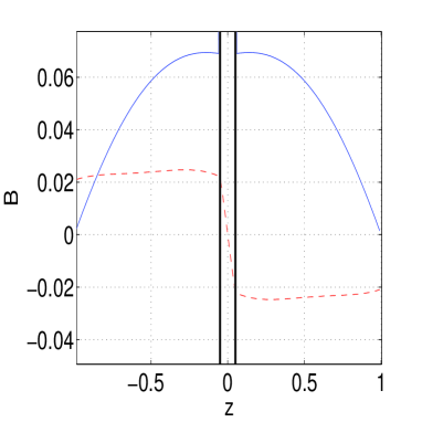
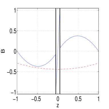
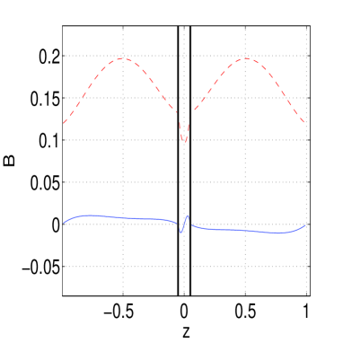
Figure 4: Eigenmodes at their onset for a symmetric configuration and $\mu_{r}=14.5$, $\sigma_{r}=1$, top: most unstable mode Rm$=6.475$. Bottom: second most unstable mode Rm$=8.17$. Real part (resp. imaginary part) are displayed on the left (resp. right). The $x$ (toroidal) component is the continuous (blue) curve. The $z$ (poloidal) component is the dashed (red) curve.

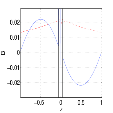
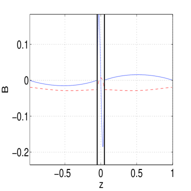
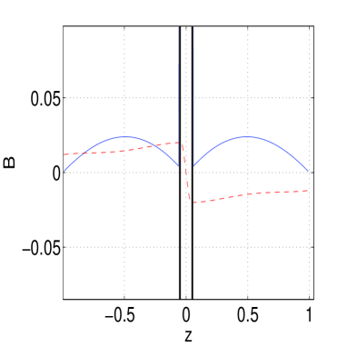
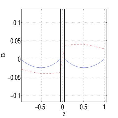
Figure 5: Eigenmodes at their onset for a symmetric configuration and $\mu_{r}=300$, $\sigma_{r}=1$, top: most unstable mode Rm$=8.36$; bottom: second most unstable mode Rm$=8.47$. Real part (resp. imaginary part) are displayed on the left (resp. right). The $x$ (toroidal) component is the continuous (blue) curve. The $z$ (poloidal) component is the dashed (red) curve.

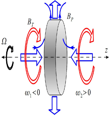
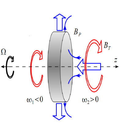
Figure 10: Sketch of the large scales of the magnetic field generated by dynamo action close to a rotating disk (angular velocity $\Omega$) of large magnetic permeability. Left: symmetric configuration, the poloidal field (blue line) changes sign from one side to the other of the disk while the toroidal field is of same sign. The disk channels the magnetic field lines so that the poloidal field changes sign on a short distance and is large even close to the disk surface. Right: asymmetric configuration, in the case where the conversion of toroidal to poloidal is small on one side of the disk, the magnetic eigenmode is expected to have a toroidal component of same sign on both sides while the poloidal is dominant on one side of the disk.

References

- (1) Chandrasekhar Hydrodynamic and hydromagnetic stability 1961, (Clarendon Press, Oxford).
- (2) Monchaux R. et al., Phys. Rev. Lett. 98, 044502 (2007).
- (3) Pétrélis F., Mordant, N. and Fauve, S. G. A. F. D. 101, 289 (2007).
- (4) Ravelet F. et al., Phys. Fluids, 17, 117104 (2005).
- (5) Moffatt H. K., Magnetic field generation in electrically conducting fluids, Cambridge University Press, Cambridge (1978).
- (6) Laguerre R. et al., Phys. Rev. Lett. 101, 104501, (2008).
- (7) Gissinger C. et al., Europhys. Lett., 82, 29001, (2008).
- (8) Busse F. H. Wicht J., G. A. F. D. 64, 135 (1972).
- (9) Giesecke A., Stefani F. Gerbeth G., Phys. Rev. Lett., 104, 044503 (2010).
- (10) Gallet B., Pétrélis F. and Fauve S., EPL 97, 69001 (2012).
- (11) Gallet B., Pétrélis F. and Fauve S., J.F.M. 27, 161-190 (2013).
- (12) Verhille G. et al., New Journal of Physics, 12 033006 (2010).