Assembly of repetitive regions using next-generation sequencing data

Abstract

High read depth can be used to assemble short sequence repeats. The existing genome assemblers fail in repetitive regions of longer than average read.

I propose a new algorithm for a DNA assembly which uses the relative frequency of reads to properly reconstruct repetitive sequences. The mathematical model shows the upper limits of accuracy of the results as a function of read coverage. For high coverage, the estimation error depends linearly on repetitive sequence length and inversely proportional to the sequencing coverage. The algorithm requires high read depth, provided by the next-generation sequencers and could use the existing data. The tests on errorless reads, generated in silico from several model genomes, pointed the properly reconstructed repetitive sequences, where existing assemblers fail.

The C++ sources, the Python scripts and the additional data are available at http://dnaasm.sourceforge.org.

1 Introduction

Next-generation sequencing (NGS) dramatically reduced the cost of producing genome sequences [1]. Therefore, we observe exponential increase of sequencing data [2]. The whole-genome shotgun method is the most popular sequencing technique, where the computer programs called genome assemblers reconstruct a DNA sequence up to chromosome length. The genome assembly is a challenging task for computer science due to a huge volume and complexity of input data produced by NGS. The huge volume of data results from both higher throughput and higher over-sampling. Computer programs use the de Bruijn graphs [3; 4] as well as greedy extensions of overlap-consensus-layout graphs [5] to process the volume of data.

Currently more than 50 genome assemblers are available [6; 7; 8; 9], but the assembly products are incomplete due to the repetitive regions, the uncovered areas and the sequencing errors. The feasibility of assembly with short reads generated from completely sequenced genomes [10] shows that there is still room for better algorithms.

The short sequence repeats (SSR) are infrequent in sequences coding proteins, therefore transcriptome analysis use genome sequences without properly restored SSR. However, SSR occur in large quantities in eukaryiotic [11] and prokaryitic cells [12], mainly in extragenic and regulatory regions and these regions are used to study genetic variations between individuals. Older techniques based on micro-array or electrophoresis have been replaced with the NGS data used to detect such variations [13; 14; 15], when the reference genome is available.

In the presented approach I propose a new algorithm to retrieve the length of an repetitive section using short reads, designed for de novo assembly of NGS data. This algorithm estimates SSR length from the coverage statistics and it is able to properly assemble consecutive repeats, as depicted in Fig. 1.

Figure 1: SSR, denoted by R, surrounded by unique sequences, denoted by A, B, C, in genome fragment. Case a and b are handled by existing sequence assemblers, case c is properly solved by the presented algorithm, case d is insolvable. Each A, B, C, R are longer than de Bruijn graph dimension.

To my knowledge, only the Euler-SR assembler[16] handles consecutive repeats of longer than average read or de Bruijn graph dimension. It constructs the assembly as a path that traverses the repeat twice, therefore underestimates the copy number. The other assemblers skip such SSR.

The paper is organized as follows: Section 2 describes the new algorithm and the mathematical model used to calculate the accuracy of SSR length estimation. Section 3 shows the numerical experiments on in silico generated data. Finally, Section 4 presents the proposals for extensions, the protocol of processing the existing data and the conclusions.

2 Approach

Algorithm

The algorithm uses a k-dimensional weighted de Bruijn multigraph $G(V,E)$, called A-Bruijn graph [17], where $V$ is a set of vertices, $E$ is a set of edges. The edge $e(u,v)$ represents the sequence $s_{0}s_{1}...s_{k-1}$, the vertex $u$, the source of edge $e$, represents the sequence $s_{0}...s_{k-2}$, the vertex $v$, the target of $e$, represents $s_{1}...s_{k-1}$. The edge weight $w$ may be understood as the number of the parallel edges between the source and the target vertices and it depicts how many times the edge should be used to produce an output path.

The algorithm is built of three steps: the graph construction from reads, the edge weight normalization and the output generation.

Alg. 1 constructs an A-Bruijn graph $G$ from a set of reads $R$. Every sub-string of length $k$ from $R$ creates an edge in $G$.

Algorithm 1 A-Bruijn graph construction algorithm

0:  $R$ collection of reads

  $G\leftarrow\emptyset$

  for all $r\in R:|r|\geq k$ do

     for all $i:0\leq i\leq|r|-k$ do

        $u\leftarrow r_{i}...r_{i+k-2}$, $v\leftarrow r_{i+1}...r_{i+k-1}$

        $G.add(edge(u,v))$ {increase edge’s weight if exists otherwise add new edge to $G$ with $w=1$}

     end for

  end for

An SSR is a sequence $S=m_{0}...m_{d-1}m_{0}...m_{(n-1)\bmod d}$, with of length $n$, $|S|=n$. $S$ is built of a repeating motif $m=m_{0}m_{1}...m_{d-1}$, $|m|=d$, $d\leq\frac{n}{2}$. Such SSR create whirls [16], when $n\geq 2(k-1)$. Some whirls are shown in Tab. 1.

	$d=1$	$d=2$	$d=3$
$\begin{array}[]{l}n-k\equiv 0\\ \pmod{d}\end{array}$
$\begin{array}[]{l}n-k\equiv 1\\ \pmod{d}\end{array}$
$\begin{array}[]{l}n-k\equiv d-1\\ \pmod{d}\end{array}$

Table 1: Examples of whirls in an A-Bruijn graph, $w$ is edge weight, $k$ is graph dimension, $d$ is motif length, $n$ is repetitive sequence length, $n\geq 2(k-1)$.

The second step of the algorithm, edge normalization, is a new approach to genome assembly. Eq. 1 converts the edge weight $w$ into $w^{\prime}$, where $c$ is sequencing coverage and $L$ is read average length. The $w^{\prime}$ may be understood as edge coverage, because the sequence with length $L$ creates $L-k+1$ fragments of length $k$ in Alg. 1.

$$w^{\prime}=\lfloor\frac{k}{c(L-k+1)}w+0.5\rfloor,\mbox{~{}where~{}}L\geq k$$ (1)

The normalization reduces errors, assuming that reads spread uniformly over the sequenced genome. The fragments that occur less frequently than $\frac{c(L-k+1)}{2k}$ are removed from A-Bruijn graph. The normalization plays a similar role to rejecting the sequences that occurs less frequently than predetermined threshold, which is used in other sequence assemblers. Moreover, it provides the relative frequency of edges, used for a proper SSR assembly.

The final step of the algorithm, output generation, depicted in Alg. 2, requires the existence of Eulerian path in A-Bruijn graph $G(V,E)$. This condition is tested by looking at all the vertices $v\in V$. If all except the initial and final vertices have an equal number of input and output edges, $\forall v\in V\setminus\{v_{0},v_{n}\}:|v.out|=|v.in|$, the initial vertex satisfies $v_{0}\in V:|v.out|-|v.in|=1$ condition, and the final vertex $v_{n}\in V:|v.out|-|v.in|=-1$, the Eulerian path exists.

Due to the presence of repetitions, graph $G$ may contain many Eulerian paths, which means ambiguity of the target sequence. Therefore, the output generation constructs a set of sub-strings of the target sequence called contigs. The contig is an Eulerian sub-path, as shown in Alg. 2.

Algorithm 2 Algorithm to construct a set of contigs from graph $G$.

0:  A-Bruijn graph $G$ with an Eulerian path, $v_{0}$ is starting vertex

  $contigs\leftarrow\emptyset$ {output of assembler}

  $v\leftarrow v_{0}$ {current vertex}

  $c\leftarrow\emptyset$ {current contig}

  loop

     if $|v.out|==0$ then

        $contigs.insert(c)$

        return  $contigs$ {end of algorithm}

     end if

     $e\leftarrow v.out[0]$ {current edge}

     if $|v.out|>1$ then

        $f\leftarrow v.out[1]$ {second current edge}

        if $|v.out|=2$ and ($isBridge(e)$ or $isBridge(f)$) then

           if $isBridge(e)$ then

              $e\leftarrow f$

           end if

        else

           $contigs.insert(c)$ {$v$ is ambiguous}

           $c\leftarrow\emptyset$

        end if

     end if

     $c.insert(e)$

     $v\leftarrow e.target$

     $G.delete(e)$ {decreases edge’s weight, if it achieves 0, remove $e$ from $G$}

  end loop

The algorithm iteratively processes all vertices $V$ starting from $v_{0}$. The current vertex $v$, if unambiguous, extends the current contig $c$, otherwise, it starts the new contig. A given vertex is unambiguous iff it has one or two output edges and, in the case when exactly two output edges exist, either is a bridge (an edge is a bridge if it has a path leading from the target vertex to the source vertex). This condition extends the test used in other existing assemblers, where ambiguity is set if the vertex has more than one output edge. Alg. 2 reduces the number of contigs in comparison with the existing assemblers, because the vertices with exactly two output edges, where one is a bridge, do not create a new contig. Time complexity of the presented algorithm is quadratic in function of the number of edges, as is the case for Fleury’s algorithm [18].

Alg. 2 uses $isBridge(e)$ procedure that checks if edge $e$ is a bridge, i.e. if it connects different strongly connected components. This procedure tries to find a path from target vertex of $e$ to source vertex of $e$ using depth first search [18].

Assembly k-spectrum

Given a string $S=s_{0}s_{1}...s_{G-1}$, $|S|=G$, let $S_{k}(i)$ be the sub-string $s_{i}...s_{i+k-1}$ of length $k\leq G$. The k-spectrum of $S$ is a set of all $S_{k}(i)$ for $0\leq i<G-k$.

The k-spectrum is idealized sequence assembler input, because all k-substrings without repetitions, errors and forward oriented are available, as depicted in Fig. 2.

Figure 2: K-spectrum construction. The reads are generated for coordinates $(0,k-1),(1,k),...,(G-k,G-1)$, where $G$ is the input sequence length.

If k-spectrum is the input of presented algorithm, the edges weights inside whirls $w$ are expressed by Eq. 2, where $n$ is SSR length, $d$ is motif length, $k$ is graph dimension. Edges inside whirls have identical value $w$ for $n-k\equiv d-1\pmod{d}$, otherwise the weight is either $w$ or $w-1$, examples are shown in Tab. 1. In further we assume, for simplicity, that $n-k\equiv d-1\pmod{d}$.

$$w=\frac{\Delta}{d},\mbox{~{}where }\Delta\equiv 0\pmod{d},\Delta=n-k+1$$ (2)

The presented algorithm is able to reconstruct SSR of any length from k-spectrum. Eq. 3 expresses repetitive sequence length from whirls parameters, Tab. 2 shows some examples.

$$n=wd+k-1,\mbox{~{}where }n-k\equiv d-1\pmod{d}$$ (3)

AAAAAAA	ATATATA	ATTATT

Table 2: Examples of whirls in 4-dimensional A-Bruijn graph and SSR reconstructed using Eq. 3

The ability of SSR reconstruction by the presented algorithm was checked on generated sequences. The k-spectrum from these sequences was used as an input for the presented computer program and the three existing genome assemblers based on de Bruijn graph, are described in Section 3. Only the presented algorithm properly reconstructs the input, as depicted in Tab. 3.

Assembly error-less uniformly distributed reads

In this section, the randomly spread fragments are regarded to be the input. All reads have the same length $L\geq k$, the distribution of the initial positions is uniform, the reads are properly oriented in the forward direction and the sequences have no errors.

This set of reads is closer to reality than k-spectrum, considered before, all consecutive sub-strings are not required, the read length is not equal to graph dimension $k$. The presented input is used to model the algorithm properties.

The reads are uniformly spread over the input genome sequence of length $G$, therefore the probability $p$ of choosing fragment of length $k$ is $\frac{1}{G-L}\approx\frac{1}{G}\mbox{~{}for~{}}G\gg L$, where $L$ is the length of read. The sequences assigned to the edges inside whirls are created from SSR, and the probability of choosing such a sequence is $p=\frac{\Delta}{dG},\Delta=n-k+1$, where $d$ is the length of motif and $n$ the length of SSR. The weight of edge inside whirls $w$ is random variable with bi-nominal distribution, because the reads are independent. For $N$ reads, graph construction algorithm (Alg. 1) creates $N^{\prime}=N(L-k+1)$ of sequences, which allows to depict weight distribution $W$ as shown in Eq. 4.

$$\begin{array}[]{l}W\sim B(N^{\prime},p)\\ \mbox{~{}where~{}}N^{\prime}=N(L-k+1),p=\frac{\Delta}{dG},\Delta=n-k+1\end{array}$$ (4)

In real cases, the random variable $W$ depicted in Eq. 4 could be estimated by Poisson distribution, with $\lambda=N^{\prime}p$, as depicted in Eq. 5, because $p\ll 1$ ($G\gg 1$) and the number of input fragments is big ($N\gg 1,L\geq k$). The $c$ is sequence redundancy $c=\frac{LN}{G}$. The parameter $c^{\prime}=\frac{c(L-k+1)}{k}$ may be understood as edge redundancy, the frequency of the sequence corresponding to the edge is in the output of Alg. 1.

$$\begin{array}[]{l}W\sim\operatorname{Poisson}\left({\lambda}\right)\\ \mbox{~{}where~{}}\lambda=\frac{c^{\prime}\Delta}{d},c^{\prime}=\frac{c(L-k+1)}{k},\Delta=n-k+1\end{array}$$ (5)

Error estimation of edge weight normalization

The edge’s weight $w$ is normalized, then rounded, as depicted in Eq. 1, to account for the reading coverage in the assembly algorithm.

The repetitive sequence length $\hat{n}$ could be estimated from A-Bruijn graph whirls parameters by using Eq. 6, where $w^{\prime}$ is normalized edge’s weight, $k$ is graph dimension, $d$ is motif length. This relation is similar to Eq. 2 defined for k-spectrum input.

$$\hat{n}=w^{\prime}d+k-1,\mbox{~{}where~{}}n-k\equiv d-1\pmod{d}$$ (6)

The probability of getting $w^{\prime}$ that allows to determine accurately the length of SSR is depicted in Eq. 7, where $\Phi_{P}(x,\lambda)$ is cumulative distribution function for Poisson distribution with parameter $\lambda$. This relation is depicted in Fig. 3.

$$\begin{array}[]{l}P(w^{\prime}=\frac{n-k+1}{d})=\Phi_{P}(\lambda+\frac{c^{\prime}}{2},\lambda)-\Phi_{P}(\lambda-\frac{c^{\prime}}{2},\lambda)\\ \mbox{~{}where~{}}\lambda,c^{\prime}\mbox{~{}are defined in Eq.~{}\ref{eqPoisson}}\end{array}$$ (7)

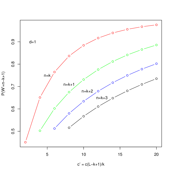
Figure 3: The probability of proper SSR length estimation in the function of coverage. The Eq. 7 was used for single symbol repetitions.

The probability mass function of a variable with Poisson distribution is asymmetrical: it is high on the left and skewed towards the right, therefore the rounding error made at the right end of the interval is larger than at the left end. It advises not to use rounding to the nearest integer (as depicted in Eq. 1).

The repetitive sequence length, estimated by Eq. 6, is inside the interval defined by Eq. 8, where $0\leq q\leq 1$ is a defined level of confidence, $\Phi^{-1}_{P}(q,\lambda)$ is an inverse cumulative distribution function for Poisson distribution with parameter $\lambda$, $\hat{n}_{max}$ is an upper boundary of repetitive sequence length, $\hat{n}_{min}$ is a lower boundary of repetitive sequence length. The intervals are depicted in Fig. 4.

$$\left.\begin{array}[]{ll}\hat{n}_{max}&=\frac{1}{c^{\prime}}\Phi^{-1}_{P}(\frac{1+q}{2},\lambda)\\ \hat{n}_{min}&=\frac{1}{c^{\prime}}\Phi^{-1}_{P}(\frac{1-q}{2},\lambda)\end{array}\right\}\mbox{~{}where~{}}\lambda,c^{\prime}\mbox{~{}are defined in Eq.~{}\ref{eqPoisson}}$$ (8)

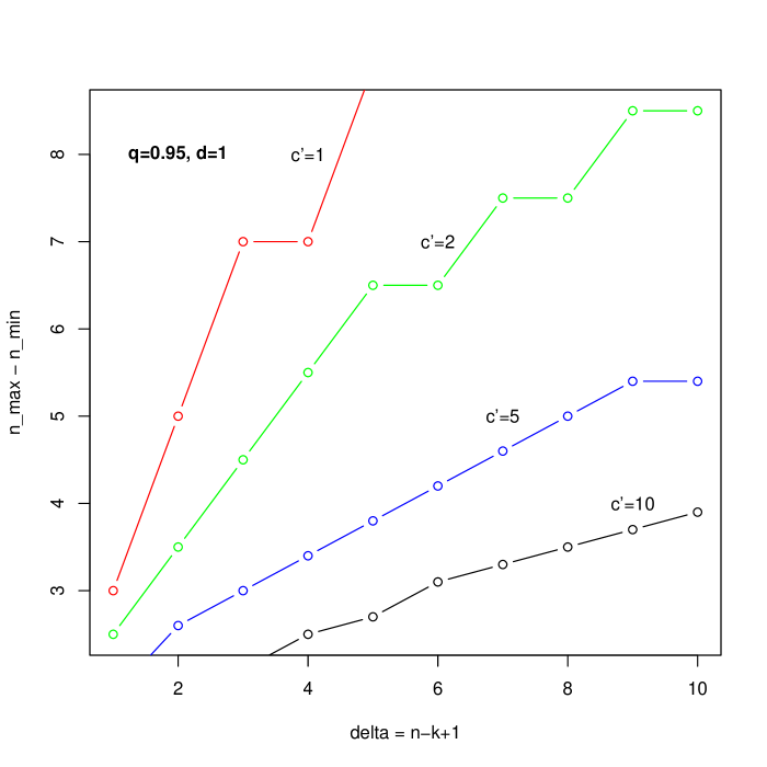
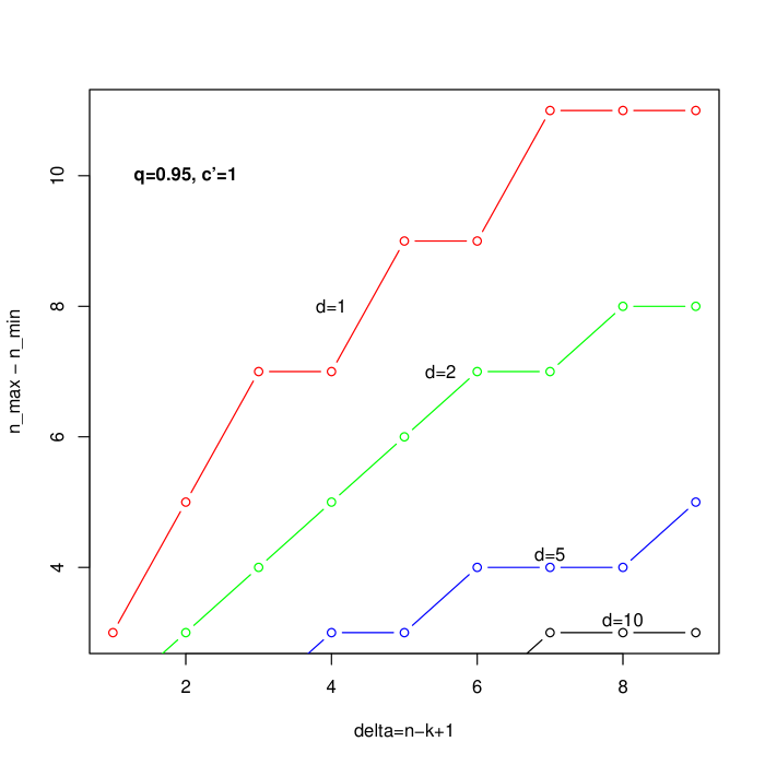
Figure 4: The interval size ($\hat{n}_{max}-\hat{n}_{min}$ from Eq. 8) of estimated SSR length for $0.95$ confidence level.

Calculating the required sequencing coverage

The SSR length estimation requires high coverage, as depicted in Fig. 3, where $P(w^{\prime}=\frac{n-k+1}{d})\geq 0.9$ for $c^{\prime}>10$. For high coverage, the Poisson distribution of edge’s weight, Eq. 5, can be approximated by Normal distribution, as depicted in Eq. 9, where $\mu$ is a mean, $\sigma$ is a standard deviation.

$$W^{\prime}\sim\mathcal{N}(\mu,\sigma)\mbox{~{}where~{}}\mu=\frac{\Delta}{d},\sigma=\sqrt{\frac{\Delta}{d}},\Delta=n-k+1$$ (9)

In this case the required coverage is linearly dependent on the repetitive sequence length $n$, as depicted in Eq. 10 and Fig. 5, where $\Phi_{N}^{-1}(q)$ is the inverse cumulative distribution function for standard normal distribution ($\mu=0$, $\sigma=1$), $q$ is required confidence level.

$$c^{\prime}=(2\Phi_{N}^{-1}(\frac{1+q}{2}))^{2}\frac{\Delta k}{d}\mbox{~{}where~{}}\Delta=n-k+1$$ (10)

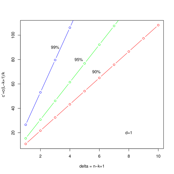
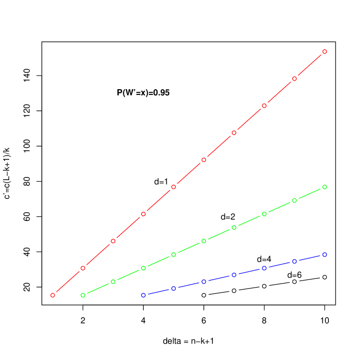
Figure 5: The required edge coverage $c^{\prime}$ for high values of confidence level in function of SSR length.

This model is useful in planning genome assembly experiments, for example, to achieve estimation of the length of the repetitive sequences of $d=5$ and $n=150$ with 95% confidence interval, when the average read length is $L=80$, the de Bruijn graph dimension $k=50$, we should use $c^{\prime}\geq 307$, therefore $c\geq 495$. If the $30\times$ coverage is used ($c=30,c^{\prime}=\frac{c(L-k+1)}{k}=31$) the length of repetitive sequence of $d=5$ and $n=150$ is in interval $\hat{n}\in(146,154)$ with 95% probability.

3 Methods

Reconstruct generated SSR

The numerical experiments prove the ability to reconstruct SSR properly by the presented algorithm. The $18$ different input sequences were generated by Python script. These sequences can be described by patterns $A$, $AR$, $ARB$, where the $A$, $B$ and $R$ are sequences of length $1000$ and $10000$, $A$ and $B$ are unique without SSR, $R$ is SSR with a motif of length $d=1,2,4,10$. The k-spectrum for each sequence mentioned above were generated and used as input for presented algorithm, ABySS [19], ver. 1.3.7 genome assembler, MIRA[20], ver. 4.0 and Velvet[21] ver. 1.2.10. Each input was performed 3 times for each assembler, to eliminate the randomness. Tab. 3 summarizes the results: the presented approach properly assembles SSR longer than graph dimension, the other assemblers are unable to assemble the repetitive sequences.

sequence	presented	ABySS	MIRA	Velvet
$A$	+	+	+	+
$AR$	+	-	-	-
$ARB$	+	-	-	-

Table 3: The successful reconstruction of generated sequence from its k-spectrum. $A,B$ are long, unique, non-repetitive sequences, $R$ is long SSR, $|A|=|B|=|R|=1000$ or $|A|=|B|=|R|=10000$, motif length is $1,2,4$ or $10$.

Assembly k-spectrum generated from model genomes

The existing genome sequences of model species: Escherichia coli (536 genome, GenBank NC_008253), Saccharomyces cerevisiae (S288c genome, version R64, GenBank NC_001133 …NC_001148, NC_001224), Arabidopsis thialina (TAIR9, The Arabidopsis Information Resource http://arabidopsis.org), and Homo sapiens (GRCh37, release 75, http://www.ensembl.org) were investigated to check the regions properly assembled by the presented algorithm.

Firstly, the k-spectrum, where $k=51$ was generated for each chromosome; secondly, the assembler was used to reconstruct the sequence. The number of places where the presented algorithm properly assembles the sequence and a typical algorithm fails was counted. The results are depicted in Tab. 4.

The presented algorithm achieves approximately 5% less contig numbers than other assemblers. Tab. 5 and Tab. 6 depicts examples of properly reconstructed SSR.

name	no. of places
e.coli, Escherichia coli	53
yeast, Saccharomyces cerevisiae	301
arabidopsis, Arabidopsis thialina	2911
human, Homo sapiens, chr. XIII – XXII	15565

Table 4: Number of places where our algorithm works properly and other sequence assemblers fail. The reads were generated from model genomes.

position (index)	motif	length
e.coli, 2066694	ACAGATAC	80
yeast, chr.II, 464020	GTT	83
yeast, chr.IV, 778759	TTA	71
yeast, chr.VII, 280054	GAGGTTGCTGTT	110
yeast, chr.XIII, 86952	TTA	118
arabid., chr.I, 17882880	ATC	125
arabid., chr.I, 18486514	TGTA	135
arabid., chr.II, 2758565	TTCTATG	130
arabid., chr.II, 5401576	TTA	145
arabid., chr.II, 16723214	CAGTCT	135
arabid., chr.III, 1818686	TAA	71
arabid., chr.III, 6375808	ATGGGG	86
arabid., chr.IV, 2488534	AAGACGAAGAAG	90
arabid., chr.V, 7614543	TACA	82
arabid., chr.V, 20395151	TAA	180
arabid., chr.V, 24022835	TCC	140

Table 5: SSR properly assembled from k-spectrum generated from e.coli (Escherichia coli), yeast (Saccharomyces cerevisiae), arabidopsis (Arabidopsis thialina) genomes, where $k=51$. The table depicts SSR longer than $70$ of motif length $d\leq 12$.

chr.	index	motif	length
XIII	29027164	TTTCC	135
XIII	49892614	GGAAAG	167
XIII	44716268	CTCGG	180
XIII	102813925	AGA	152
XV	65438307	TAAATATATATA	161
XV	69970764	CTTTC	105
XVII	5185392	CGCGCTCCCTC	109
XVII	20460059	TCCCTC	149
XVII	4365394	TCCA	533
XVII	77867600	ATC	239
XVII	78639134	TTCCT	170
XVIII	47105376	AGAGGG	233
XVIII	49836110	ATATATATTTCT	112
XVIII	62056751	CTTTC	125
XIX	53422228	CTCCCT	194
XIX	57993815	CTCTCCC	120
XXI	40955746	CCTT	254
XXII	16288601	CGGCGTGCGCGTG	102
XXII	27691662	ATGG	102

Table 6: SSR properly assembled from k-spectrum generated from human genome (Homo sapiens), chromosomes XIII – XXII, where $k=51$. The table depicts SSR longer than $100$ of motif length $d\leq 12$.

4 Discussion and conclusion

The presented algorithm uses the short read data more efficiently than other computer programs when high coverage is available. It is able to assemble properly some repetitive sequences, and achieve 5% better contig size, if used on k-spectrum generated from model genomes.

This assembler is able to use reads of different lengths, if the length is greater than graph dimension $k$. If you are using collections of readings of different lengths, e.g. from different experiments, the fragment length $L$ should be replaced by arithmetic mean $\bar{L}$ in Eq. 4, Eq. 5, Eq. 7 and Eq. 8.

The existing genome drafts, especially for plant genomes, are not fully assembled, inter alia, due to a large number of SSR. The presented algorithm could reduce gaps in the existing data. The procedure includes finding the repetitive sequences in contigs ends. If two and only two contigs have the same SSR at the end, they could be connected to create a single contig. The SSR length is estimated by Eq. 6 with accuracy expressed in Eq. 8.

To obtain the length of repetitive sequence with a big confidence level, higher than typical coverage should be applied ($c>100$). If the required coverage is beyond the project funds, it should be considered in future genome sequencing projects, as the cost decreases exponentially.

The mathematical model proposed in this paper is the upper limit of the calculation accuracy, because the distribution of read start positions deviates from uniformity and contains sequencing errors. The big coverage required by the presented approach, when normal distribution describes the edge’s weight, permit the underlying distribution different from uniform. However, the special sequences, underestimated and overestimated with the sequencing technology should be considered. We plan to review the technology to find such sequences and take this into account in the next version of software.

The sequencing errors are corrected in the presented approach by edge normalization process (Eq. 1). The other error awareness techniques are considered in future versions of presented software: incorporate sequence quality into assembly algorithm and correction of systematic errors created by next-generation sequencers. Moreover, the improper assembly output could be corrected when information of k-mer position generated from read is used [22].

The key improvement in assembly results, especially for de Bruijn graph based solutions, is the usage of the new experimental opportunity, called mate pairs. The sequencers are able to read the pairs of sequences between which the genomic distance is well estimated. The mate pairs could link contigs into scaffolds, and are used either as post-processing steps [23; 21; 24] or as internal assembler process where connections are incorporated into the graph structure [25]. Mate pairs, in theory, allow to properly assemble the sequences of length equal to the sum of lengths of known sequences on both ends and length of the distance. It significantly increases the effective length of reads, because the distance could be long. The mate pairs were successfully used to de novo assemble highly repetitive telomeric regions [26].

The presented algorithm currently does not use mate pair data; however, the integration of such data is one of the most important tasks in the next version of software.

The presented algorithm assumes forward orientation of all readings, i.e. the reads come from only one DNA strand. In real data both coding and complementary DNA strand provide reads. The further version of computer program will include the sequence and complementary in node representation, similarly to the Velvet assembler [21].

In conclusion, the proposed solution better assembles short sequence repeats than other sequence assemblers. The proposed mathematical model estimates the coverage to achieve the required level of confidence. The length of properly reconstructed SSR linearly depends on genome coverage.

References

- [1] J. Shendure, H. Ji, Next-generation dna sequencing, Nature biotechnology 26 (10) (2008) 1135–1145.
- [2] I. Pagani, K. Liolios, J. Jansson, I.-M. A. Chen, T. Smirnova, B. Nosrat, V. M. Markowitz, N. C. Kyrpides, The genomes online database (gold) v. 4: status of genomic and metagenomic projects and their associated metadata, Nucleic acids research 40 (D1) (2012) D571–D579.
- [3] P. A. Pevzner, H. Tang, M. S. Waterman, An eulerian path approach to dna fragment assembly, Proceedings of the National Academy of Sciences 98 (17) (2001) 9748–9753.
- [4] E. W. Myers, The fragment assembly string graph, Bioinformatics 21 (suppl 2) (2005) ii79–ii85.
- [5] J. R. Miller, S. Koren, G. Sutton, Assembly algorithms for next-generation sequencing data, Genomics 95 (6) (2010) 315–327.
- [6] W. Zhang, J. Chen, Y. Yang, Y. Tang, J. Shang, B. Shen, A practical comparison of de novo genome assembly software tools for next-generation sequencing technologies, PloS one 6 (3) (2011) e17915.
- [7] D. Earl, K. Bradnam, J. S. John, A. Darling, D. Lin, J. Fass, H. O. K. Yu, V. Buffalo, D. R. Zerbino, M. Diekhans, et al., Assemblathon 1: A competitive assessment of de novo short read assembly methods, Genome research 21 (12) (2011) 2224–2241.
- [8] K. R. Bradnam, J. N. Fass, A. Alexandrov, P. Baranay, M. Bechner, I. Birol, S. Boisvert, J. A. Chapman, G. Chapuis, R. Chikhi, et al., Assemblathon 2: evaluating de novo methods of genome assembly in three vertebrate species, GigaScience 2 (1) (2013) 1–31.
- [9] S. L. Salzberg, A. M. Phillippy, A. Zimin, D. Puiu, T. Magoc, S. Koren, T. J. Treangen, M. C. Schatz, A. L. Delcher, M. Roberts, et al., Gage: A critical evaluation of genome assemblies and assembly algorithms, Genome research 22 (3) (2012) 557–567.
- [10] C. Kingsford, M. C. Schatz, M. Pop, Assembly complexity of prokaryotic genomes using short reads, BMC bioinformatics 11 (1) (2010) 21.
- [11] R. Cox, S. M. Mirkin, Characteristic enrichment of dna repeats in different genomes, Proceedings of the National Academy of Sciences 94 (10) (1997) 5237–5242.
- [12] A. van Belkum, S. Scherer, L. van Alphen, H. Verbrugh, Short-sequence dna repeats in prokaryotic genomes, Microbiology and Molecular Biology Reviews 62 (2) (1998) 275–293.
- [13] M. D. Cao, E. Tasker, K. Willadsen, M. Imelfort, S. Vishwanathan, S. Sureshkumar, S. Balasubramanian, M. Bodén, Inferring short tandem repeat variation from paired-end short reads, Nucleic acids research (2013) gkt1313.
- [14] C. Xie, M. T. Tammi, Cnv-seq, a new method to detect copy number variation using high-throughput sequencing, BMC bioinformatics 10 (1) (2009) 80.
- [15] S. Yoon, Z. Xuan, V. Makarov, K. Ye, J. Sebat, Sensitive and accurate detection of copy number variants using read depth of coverage, Genome research 19 (9) (2009) 1586–1592.
- [16] M. J. Chaisson, P. A. Pevzner, Short read fragment assembly of bacterial genomes, Genome research 18 (2) (2008) 324–330.
- [17] P. Pevzner, H. Tang, G. Tesler, De novo repeat classification and fragment assembly, Genome Research 14 (9) (2004) 1786–1796.
- [18] T. Cormen, C. Leiserson, R. Rivest, C. Stein, Introduction to algorithms, The MIT press, 2001.
- [19] J. T. Simpson, K. Wong, S. D. Jackman, J. E. Schein, S. J. Jones, İ. Birol, Abyss: a parallel assembler for short read sequence data, Genome research 19 (6) (2009) 1117–1123.
- [20] B. Chevreux, T. Wetter, S. Suhai, Genome sequence assembly using trace signals and additional sequence information., in: German Conference on Bioinformatics, 1999, pp. 45–56.
- [21] D. R. Zerbino, E. Birney, Velvet: algorithms for de novo short read assembly using de bruijn graphs, Genome research 18 (5) (2008) 821–829.
- [22] R. Ronen, C. Boucher, H. Chitsaz, P. Pevzner, Sequel: improving the accuracy of genome assemblies, Bioinformatics 28 (12) (2012) i188–i196.
- [23] J. Butler, I. MacCallum, M. Kleber, I. A. Shlyakhter, M. K. Belmonte, E. S. Lander, C. Nusbaum, D. B. Jaffe, Allpaths: de novo assembly of whole-genome shotgun microreads, Genome research 18 (5) (2008) 810–820.
- [24] P. Piotrowski, R. Nowak, New tool to combine contigs by usage of paired-end tags, in: Photonics Applications in Astronomy, Communications, Industry, and High-Energy Physics Experiments 2013, International Society for Optics and Photonics, 2013, pp. 890318–890318.
- [25] P. Medvedev, S. Pham, M. Chaisson, G. Tesler, P. Pevzner, Paired de bruijn graphs: a novel approach for incorporating mate pair information into genome assemblers, Journal of Computational Biology 18 (11) (2011) 1625–1634.
- [26] M. Bresler, S. Sheehan, A. H. Chan, Y. S. Song, Telescoper: de novo assembly of highly repetitive regions, Bioinformatics 28 (18) (2012) i311–i317.