Abstract

We study randomized sketching methods for approximately solving least-squares problem with a general convex constraint. The quality of a least-squares approximation can be assessed in different ways: either in terms of the value of the quadratic objective function (cost approximation), or in terms of some distance measure between the approximate minimizer and the true minimizer (solution approximation). Focusing on the latter criterion, our first main result provides a general lower bound on any randomized method that sketches both the data matrix and vector in a least-squares problem; as a surprising consequence, the most widely used least-squares sketch is sub-optimal for solution approximation. We then present a new method known as the iterative Hessian sketch, and show that it can be used to obtain approximations to the original least-squares problem using a projection dimension proportional to the statistical complexity of the least-squares minimizer, and a logarithmic number of iterations. We illustrate our general theory with simulations for both unconstrained and constrained versions of least-squares, including $\ell_{1}$-regularization and nuclear norm constraints. We also numerically demonstrate the practicality of our approach in a real face expression classification experiment.

1 Introduction

Over the past decade, the explosion of data volume and complexity has led to a surge of interest in fast procedures for approximate forms of matrix multiplication, low-rank approximation, and convex optimization. One interesting class of problems that arise frequently in data analysis and scientific computing are constrained least-squares problems. More specifically, given a data vector $y\in\mathbb{R}^{n}$, a data matrix $A\in\mathbb{R}^{n\times d}$ and a convex constraint set $\mathcal{C}$, a constrained least-squares problem can be written as follows

$$x^{\mbox{\tiny{LS}}} :\,=\arg\min_{x\in\mathcal{C}}f(x)\qquad\mbox{where $f(x):\,=\frac{1}{2n}\|Ax-y\|_{2}^{2}$.}$$ (1)

The simplest case is the unconstrained form ($\mathcal{C}=\mathbb{R}^{d}$), but this class also includes other interesting constrained programs, including those based $\ell_{1}$-norm balls, nuclear norm balls, interval constraints $[-1,1]^{d}$ and other types of regularizers designed to enforce structure in the solution.

Randomized sketches are a well-established way of obtaining an approximate solutions to a variety of problems, and there is a long line of work on their uses (e.g., see the books and papers [38, 8, 25, 16, 21], as well as references therein). In application to problem (1), sketching methods involving using a random matrix $S\in\mathbb{R}^{m\times n}$ to project the data matrix $A$ and/or data vector $y$ to a lower dimensional space ($m\ll n$), and then solving the approximated least-squares problem. There are many choices of random sketching matrices; see Section 2.1 for discussion of a few possibilities. Given some choice of random sketching matrix $S$, the most well-studied form of sketched least-squares is based on solving the problem

$$\widetilde{x} :\,=\arg\min_{x\in\mathcal{C}}\Big{\{}\frac{1}{2n}\|SAx-Sy\|_{2}^{2}\Big{\}},$$ (2)

in which the data matrix-vector pair $(A,y)$ are approximated by their sketched versions $(SA,Sy)$. Note that the sketched program is an $m$-dimensional least-squares problem, involving the new data matrix $SA\in\mathbb{R}^{m\times d}$. Thus, in the regime $n\gg d$, this approach can lead to substantial computational savings as long as the projection dimension $m$ can be chosen substantially less than $n$. A number of authors (e.g., [8, 16, 25, 31]) have investigated the properties of this sketched solution (2), and accordingly, we refer to to it as the classical least-squares sketch.

There are various ways in which the quality of the approximate solution $\widetilde{x}$ can be assessed. One standard way is in terms of the minimizing value of the quadratic cost function $f$ defining the original problem (1), which we refer to as cost approximation. In terms of $f$-cost, the approximate solution $\widetilde{x}$ is said to be $\varepsilon$-optimal if

$$f(x^{\mbox{\tiny{LS}}})\;\leq\;f(\widetilde{x})\;\leq\;(1+\varepsilon)^{2}f(x^{\mbox{\tiny{LS}}}).$$ (3)

For example, in the case of unconstrained least-squares ($\mathcal{C}=\mathbb{R}^{d}$) with $n>d$, it is known that with Gaussian random sketches, a sketch size $m\succsim\frac{1}{\varepsilon^{2}}d$ suffices to guarantee that $\widetilde{x}$ is $\varepsilon$-optimal with high probability (for instance, see the papers by Sarlos [35] and Mahoney [25], as well as references therein). Similar guarantees can be established for sketches based on sampling according to the statistical leverage scores [15, 14]. Sketching can also be applied to problems with constraints: Boutsidis and Drineas [8] prove analogous results for the case of non-negative least-squares considering the sketch in (2), whereas our own past work [31] provides sufficient conditions for $\varepsilon$-accurate cost approximation of least-squares problems over arbitrary convex sets based also on the form in (2).

It should be noted, however, that other notions of “approximation goodness” are possible. In many applications, it is the least-squares minimizer $x^{\mbox{\tiny{LS}}}$ itself—as opposed to the cost value $f(x^{\mbox{\tiny{LS}}})$—that is of primary interest. In such settings, a more suitable measure of approximation quality would be the $\ell_{2}$-norm $\|\widetilde{x}-x^{\mbox{\tiny{LS}}}\|_{2}$, or the prediction (semi)-norm

$$\|\widetilde{x}-x^{\mbox{\tiny{LS}}}\|_{A}:\,=\frac{1}{\sqrt{n}}\|A(\widetilde{x}-x^{\mbox{\tiny{LS}}})\|_{2}.$$ (4)

We refer to these measures as solution approximation.

Now of course, a cost approximation bound (3) can be used to derive guarantees on the solution approximation error. However, it is natural to wonder whether or not, for a reasonable sketch size, the resulting guarantees are “good”. For instance, using arguments from Drineas et al. [16], for the problem of unconstrained least-squares, it can be shown that the same conditions ensuring a $\varepsilon$-accurate cost approximation also ensure that

$$\|\widetilde{x}-x^{\mbox{\tiny{LS}}}\|_{A} \leq\varepsilon\,\sqrt{f(x^{\mbox{\tiny{LS}}})}.$$ (5)

Given lower bounds on the singular values of the data matrix $A$, this bound also yields control of the $\ell_{2}$-error.

In certain ways, the bound (5) is quite satisfactory: given our normalized definition (1) of the least-squares cost $f$, the quantity $f(x^{\mbox{\tiny{LS}}})$ remains an order one quantity as the sample size $n$ grows, and the multiplicative factor $\varepsilon$ can be reduced by increasing the sketch dimension $m$. But how small should $\varepsilon$ be chosen? In many applications of least-squares, each element of the response vector $y\in\mathbb{R}^{n}$ corresponds to an observation, and so as the sample size $n$ increases, we expect that $x^{\mbox{\tiny{LS}}}$ provides a more accurate approximation to some underlying population quantity, say $x^{*}\in\mathbb{R}^{d}$. As an illustrative example, in the special case of unconstrained least-squares, the accuracy of the least-squares solution $x^{\mbox{\tiny{LS}}}$ as an estimate of $x^{*}$ scales as $\|x^{\mbox{\tiny{LS}}}-x^{*}\|_{A}\asymp\frac{\sigma^{2}d}{n}$. Consequently, in order for our sketched solution to have an accuracy of the same order as the least-square estimate, we must set $\varepsilon^{2}\asymp\frac{\sigma^{2}d}{n}$. Combined with our earlier bound on the projection dimension, this calculation suggests that a projection dimension of the order

$$m \succsim\frac{d}{\varepsilon^{2}}\;\asymp\frac{n}{\sigma^{2}}$$

is required. This scaling is undesirable in the regime $n\gg d$, where the whole point of sketching is to have the sketch dimension $m$ much lower than $n$.

Now the alert reader will have observed that the preceding argument was only rough and heuristic. However, the first result of this paper (Theorem 1) provides a rigorous confirmation of the conclusion: whenever $m\ll n$, the classical least-squares sketch (2) is sub-optimal as a method for solution approximation. Figure 1 provides an empirical demonstration of the poor behavior of the classical least-squares sketch for an unconstrained problem.

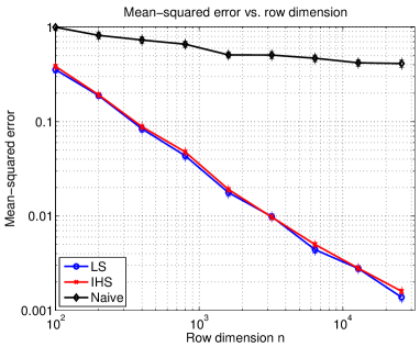
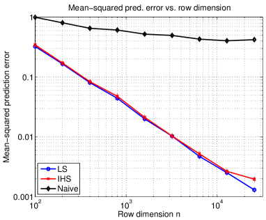
(a)	(b)

Figure 1: Plots of mean-squared error versus the row dimension $n\in\{100,200,400,\ldots,25600\}$ for unconstrained least-squares in dimension $d=10$. The blue curves correspond to the error $x^{\mbox{\tiny{LS}}}-x^{*}$ of the unsketched least-squares estimate. Red curves correspond to the IHS method applied for ${N}=1+\lceil\log(n)\rceil$ rounds using a sketch size $m=7d$. Black curves correspond to the naive sketch applied using $M={N}m$ projections in total, corresponding to the same number used in all iterations of the IHS algorithm. (a) Error $\|\widetilde{x}-x^{*}\|_{2}^{2}$. (b) Prediction error $\|\widetilde{x}-x^{*}\|_{A}^{2}=\frac{1}{n}\|A(\widetilde{x}-x^{*})\|_{2}^{2}$. Each point corresponds to the mean taken over $300$ trials with standard errors shown above and below in crosses.

This sub-optimality holds not only for unconstrained least-squares but also more generally for a broad class of constrained problems. Actually, Theorem 1 is a more general claim: any estimator based only on the pair $(SA,Sy)$—an infinite family of methods including the standard sketching algorithm as a particular case—is sub-optimal relative to the original least-squares estimator in the regime $m\ll n$. We are thus led to a natural question: can this sub-optimality be avoided by a different type of sketch that is nonetheless computationally efficient? Motivated by this question, our second main result (Theorem 2) is to propose an alternative method—known as the iterative Hessian sketch—and prove that it yields optimal approximations to the least-squares solution using a projection size that scales with the intrinsic dimension of the underlying problem, along with a logarithmic number of iterations. The main idea underlying iterative Hessian sketch is to obtain multiple sketches of the data $(S^{1}A,...,S^{N}A)$ and iteratively refine the solution where $N$ can be chosen logarithmic in $n$.

The remainder of this paper is organized as follows. In Section 2, we begin by introducing some background on classes of random sketching matrices, before turning to the statement of our lower bound (Theorem 1) on the classical least-squares sketch (2). We then introduce the Hessian sketch, and show that an iterative version of it can be used to compute $\varepsilon$-accurate solution approximations using $\log(1/\varepsilon)$-steps (Theorem 2). In Section 3, we illustrate the consequences of this general theorem for various specific classes of least-squares problems, and we conclude with a discussion in Section 4. The majority of our proofs are deferred to the appendices.

Notation:

For the convenience of the reader, we summarize some standard notation used in this paper. For sequences $\{a_{t}\}_{t=0}^{\infty}$ and $\{b_{t}\}_{t=0}^{\infty}$, we use the notation $a_{t}\preceq b_{t}$ to mean that there is a constant (independent of $t$) such that $a_{t}\leq C\,b_{t}$ for all $t$. Equivalently, we write $b_{t}\succeq a_{t}$. We write $a_{t}\asymp b_{t}$ if $a_{t}\preceq b_{t}$ and $b_{t}\preceq a_{t}$.

2 Main results

In this section, we begin with background on different classes of randomized sketches, including those based on random matrices with sub-Gaussian entries, as well as those based on randomized orthonormal systems and random sampling. In Section 2.2, we prove a general lower bound on the solution approximation accuracy of any method that attempts to approximate the least-squares problem based on observing only the pair $(SA,Sy)$. This negative result motivates the investigation of alternative sketching methods, and we begin this investigation by introducing the Hessian sketch in Section 2.3. It serves as the basic building block of the iterative Hessian sketch (IHS), which can be used to construct an iterative method that is optimal up to logarithmic factors.

2.1 Different types of randomized sketches

Various types of randomized sketches are possible, and we describe a few of them here. Given a sketching matrix $S$, we use $\{s_{i}\}_{i=1}^{m}$ to denote the collection of its $n$-dimensional rows. We restrict our attention to sketch matrices that are zero-mean, and that are normalized so that $\mathbb{E}[S^{T}S/m]=I_{n}$.

Sub-Gaussian sketches:

The most classical sketch is based on a random matrix $S\in\mathbb{R}^{m\times n}$ with i.i.d. standard Gaussian entries. A straightforward generalization is a random sketch with i.i.d. sub-Gaussian rows. In particular, a zero-mean random vector $s\in\mathbb{R}^{n}$ is $1$-sub-Gaussian if for any $u\in\mathbb{R}^{n}$, we have

$$\mathbb{P}[\langle s,\,u\rangle\geq\varepsilon\|u\|_{2}\big{]} \leq e^{-\varepsilon^{2}/2}\qquad\mbox{for all $\varepsilon\geq 0$.}$$ (6)

For instance, a vector with i.i.d. $N(0,1)$ entries is $1$-sub-Gaussian, as is a vector with i.i.d. Rademacher entries (uniformly distributed over $\{-1,+1\}$). Suppose that we generate a random matrix $S\in\mathbb{R}^{m\times n}$ with i.i.d. rows that are zero-mean, $1$-sub-Gaussian, and with $\operatorname{cov}(s)=I_{n}$; we refer to any such matrix as a sub-Gaussian sketch. As will be clear, such sketches are the most straightforward to control from the probabilistic point of view. However, from a computational perspective, a disadvantage of sub-Gaussian sketches is that they require matrix-vector multiplications with unstructured random matrices. In particular, given an data matrix $A\in\mathbb{R}^{n\times d}$, computing its sketched version $SA$ requires $\mathcal{O}(mnd)$ basic operations in general (using classical matrix multiplication).

Sketches based on randomized orthonormal systems (ROS):

The second type of randomized sketch we consider is randomized orthonormal system (ROS), for which matrix multiplication can be performed much more efficiently.

In order to define a ROS sketch, we first let $H\in\mathbb{R}^{n\times n}$ be an orthonormal matrix with entries $H_{ij}\in[-\frac{1}{\sqrt{n}},\frac{1}{\sqrt{n}}]$. Standard classes of such matrices are the Hadamard or Fourier bases, for which matrix-vector multiplication can be performed in $\mathcal{O}(n\log n)$ time via the fast Hadamard or Fourier transforms, respectively. Based on any such matrix, a sketching matrix $S\in\mathbb{R}^{m\times n}$ from a ROS ensemble is obtained by sampling i.i.d. rows of the form

$$s^{T} =\sqrt{n}e_{j}^{T}HD\qquad\mbox{with probability $1/n$ for $j=1,\ldots,n$},$$

where the random vector $e_{j}\in\mathbb{R}^{n}$ is chosen uniformly at random from the set of all $n$ canonical basis vectors, and $D=\operatorname{diag}(\nu)$ is a diagonal matrix of i.i.d. Rademacher variables $\nu\in\{-1,+1\}^{n}$. Given a fast routine for matrix-vector multiplication, the sketched data $(SA,Sy)$ can be formed in $\mathcal{O}(n\,d\log m)$ time (for instance, see the paper [1]).

Sketches based on random row sampling:

Given a probability distribution $\{p_{j}\}_{j=1}^{n}$ over $[n]=\{1,\ldots,n\}$, another choice of sketch is to randomly sample the rows of the extended data matrix $\begin{bmatrix}A&y\end{bmatrix}$ a total of $m$ times with replacement from the given probability distribution. Thus, the rows of $S$ are independent and take on the values

$$s^{T} =\frac{e_{j}}{\sqrt{p_{j}}}\qquad\mbox{with probability $p_{j}$ for $j=1,\ldots,n$}$$

where $e_{j}\in\mathbb{R}^{n}$ is the $j^{th}$ canonical basis vector. Different choices of the weights $\{p_{j}\}_{j=1}^{n}$ are possible, including those based on the leverage values of $A$—i.e., $p_{j}\propto\|u_{j}\|_{2}$ for $j=1,\ldots,n$, where $U\in\mathbb{R}^{n\times d}$ is the matrix of left singular vectors of $A$ [15]. In our analysis of lower bounds to follow, we assume that the weights are $\alpha$-balanced, meaning that

$$\max_{j=1,\ldots,n}p_{j} \leq\frac{\alpha}{n}$$ (7)

for some constant $\alpha$ independent of $n$.

In the following section, we present a lower bound that applies to all the three kinds of sketching matrices described above.

2.2 Sub-optimality of classical least-squares sketch

We begin by proving a lower bound on any estimator that is a function of the pair $(SA,Sy)$. In order to do so, we consider an ensemble of least-squares problems, namely those generated by a noisy observation model of the form

$$y =Ax^{*}+w,\qquad\mbox{where $w\sim N(0,\sigma^{2}I_{n})$,}$$ (8)

the data matrix $A\in\mathbb{R}^{n\times d}$ is fixed, and the unknown vector $x^{*}$ belongs to some compact subset $\mathcal{C}_{0}\subseteq\mathcal{C}$. In this case, the constrained least-squares estimate $x^{\mbox{\tiny{LS}}}$ from equation (1) corresponds to a constrained form of maximum-likelihood for estimating the unknown regression vector $x^{*}$. In Appendix D, we provide a general upper bound on the error $\mathbb{E}[\|x^{\mbox{\tiny{LS}}}-x^{*}\|_{A}^{2}]$ in the least-squares solution as an estimate of $x^{*}$. This result provides a baseline against which to measure the performance of a sketching method: in particular, our goal is to characterize the minimal projection dimension $m$ required in order to return an estimate $\widetilde{x}$ with an error guarantee $\|\widetilde{x}-x^{\mbox{\tiny{LS}}}\|_{A}\approx\|x^{\mbox{\tiny{LS}}}-x^{*}\|_{A}$. The result to follow shows that unless $m\geq n$, then any method based on observing only the pair $(SA,Sy)$ necessarily has a substantially larger error than the least-squares estimate. In particular, our result applies to an arbitrary measureable function $(SA,Sy)\mapsto x^{\dagger}$, which we refer to as an estimator.

More precisely, our lower bound applies to any random matrix $S\in\mathbb{R}^{m\times n}$ for which

$$|\!|\!|\mathbb{E}\Big{[}S^{T}(SS^{T})^{-1}S\Big{]}|\!|\!|_{{\mbox{\tiny{op}}}}\leq\eta\;\frac{m}{n},$$ (9)

where $\eta$ is a constant independent of $n$ and $m$, and $|\!|\!|A|\!|\!|_{{\mbox{\tiny{op}}}}$ denotes the $\ell_{2}$-operator norm (maximum eigenvalue for a symmetric matrix). In Appendix A.1, we show that these conditions hold for various standard choices, including most of those discussed in the previous section. Our lower bound also involves the complexity of the set $\mathcal{C}_{0}$, which we measure in terms of its metric entropy. In particular, for a given semi-norm $\|\cdot\|$ and tolerance $\delta>0$, the $\delta$-packing number $M_{\delta}$ of the set $\mathcal{C}_{0}$ is the largest number of vectors $\{x^{j}\}_{j=1}^{M}\subset\mathcal{C}_{0}$ such that $\|x^{j}-x^{k}\|>\delta$ for all distinct pairs $j\neq k$.

With this set-up, we have the following result:

Theorem 1 (Sub-optimality).

For any random sketching matrix $S\in\mathbb{R}^{m\times n}$ satisfying condition (9), any estimator $(SA,Sy)\mapsto x^{\dagger}$ has MSE lower bounded as

$$\sup_{x^{*}\in\mathcal{C}_{0}}\mathbb{E}_{S,w}\big{[}\|x^{\dagger}-x^{*}\|_{A}^{2}\big{]} \geq\frac{\sigma^{2}}{128\,\eta}\;\frac{\log(\frac{1}{2}M_{1/2})}{\min\{m,n\}}$$ (10)

where $M_{1/2}$ is the $1/2$-packing number of $\mathcal{C}_{0}$ in the semi-norm $\|\cdot\|_{A}$.

The proof, given in Appendix A, is based on a reduction from statistical minimax theory combined with information-theoretic bounds. The lower bound is best understood by considering some concrete examples:

Example 1 (Sub-optimality for ordinary least-squares).

We begin with the simplest case—namely, in which $\mathcal{C}=\mathbb{R}^{d}$. With this choice and for any data matrix $A$ with $\operatorname{rank}(A)=d$, it is straightforward to show that the least-squares solution $x^{\mbox{\tiny{LS}}}$ has its prediction mean-squared error at most

$$\mathbb{E}\big{[}\|x^{\mbox{\tiny{LS}}}-x^{*}\|_{A}^{2}\big{]} \precsim\>\frac{\sigma^{2}d}{n}.$$ (11a)

On the other hand, with the choice $$\mathcal{C}_{0}=\mathbb{B}_{2}(1) 1/2 M=2^{d} x^{\dagger} (SA,Sy)$$, we can construct a -packing with elements, so that Theorem 1 implies that any estimator based on has its prediction MSE lower bounded as

$$\mathbb{E}_{S,w}\big{[}\|\widehat{x}-x^{*}\|_{A}^{2}\big{]} \succsim\frac{\sigma^{2}\,d}{\min\{m,n\}}.$$ (11b)

Consequently, the sketch dimension $m$ must grow proportionally to $n$ in order for the sketched solution to have a mean-squared error comparable to the original least-squares estimate. This is highly undesirable for least-squares problems in which $n\gg d$, since it should be possible to sketch down to a dimension proportional to $\operatorname{rank}(A)=d$. Thus, Theorem 1 this reveals a surprising gap between the classical least-squares sketch (2) and the accuracy of the original least-squares estimate.

In contrast, the sketching method of this paper, known as iterative Hessian sketching (IHS), matches the optimal mean-squared error using a sketch of size $d+\log(n)$ in each round, and a total of $\log(n)$ rounds; see Corollary 2 for a precise statement. The red curves in Figure 1 show that the mean-squared errors ($\|\widehat{x}-x^{*}\|_{2}^{2}$ in panel (a), and $\|\widehat{x}-x^{*}\|_{A}^{2}$ in panel (b)) of the IHS method using this sketch dimension closely track the associated errors of the full least-squares solution (blue curves). Consistent with our previous discussion, both curves drop off at the $n^{-1}$ rate.

Since the IHS method with $\log(n)$ rounds uses a total of $T=\log(n)\big{\{}d+\log(n)\}$ sketches, a fair comparison is to implement the classical method with $T$ sketches in total. The black curves show the MSE of the resulting sketch: as predicted by our theory, these curves are relatively flat as a function of sample size $n$. Indeed, in this particular case, the lower bound (10)

$$\mathbb{E}_{S,w}\big{[}\|\widetilde{x}-x^{*}\|_{A}^{2}\big{]} \succsim\frac{\sigma^{2}d}{m}\succsim\frac{\sigma^{2}}{\log^{2}(n)},$$

showing we can expect (at best) an inverse logarithmic drop-off. $\diamondsuit$

This sub-optimality can be extended to other forms of constrained least-squares estimates as well, such as those involving sparsity constraints.

Example 2 (Sub-optimality for sparse linear models).

We now consider the sparse variant of the linear regression problem, which involves the $\ell_{0}$-“ball”

$$\mathbb{B}_{0}(s):\,=\big{\{}x\in\mathbb{R}^{d}\mid\sum_{j=1}^{d}\mathbb{I}[x_{j}\neq 0]\leq s\},$$

corresponding to the set of all vectors with at most $s$ non-zero entries. Fixing some radius $R\geq\sqrt{s}$, consider a vector $x^{*}\in\mathcal{C}_{0}:\,=\mathbb{B}_{0}(s)\cap\{\|x\|_{1}=R\}$, and suppose that we make noisy observations of the form $y=Ax^{*}+w$.

Given this set-up, one way in which to estimate $x^{*}$ is by by computing the least-squares estimate $x^{\mbox{\tiny{LS}}}$ constrained to the $\ell_{1}$-ball $\mathcal{C}=\{x\in\mathbb{R}^{n}\,\mid\,\|x\|_{1}\leq R\}$. This estimator is a form of the Lasso [37]: as shown in Appendix D.2, when the design matrix $A$ satisfies the restricted isometry property (see [10] for a definition), then it has MSE at most

$$\mathbb{E}\big{[}\|x^{\mbox{\tiny{LS}}}-x^{*}\|_{A}^{2}\big{]} \precsim\frac{\sigma^{2}s\log\big{(}\frac{ed}{s}\big{)}}{n}.$$ (12a)

On the other hand, the $\frac{1}{2}$-packing number $M$ of the set $\mathcal{C}_{0}$ can be lower bounded as $\log M\succsim s\log\big{(}\frac{ed}{s}\big{)}$; see Appendix D.2 for the details of this calculation. Consequently, in application to this particular problem, Theorem 1 implies that any estimator $x^{\dagger}$ based on the pair $(SA,Sy)$ has mean-squared error lower bounded as

$$\mathbb{E}_{w,S}\big{[}\|x^{\dagger}-x^{*}\|_{A}^{2}\big{]} \succsim\frac{\sigma^{2}s\log\big{(}\frac{ed}{s}\big{)}}{\min\{m,n\}}.$$ (12b)

Again, we see that the projection dimension $m$ must be of the order of $n$ in order to match the mean-squared error of the constrained least-squares estimate $x^{\mbox{\tiny{LS}}}$ up to constant factors. By contrast, in this special case, the sketching method developed in this paper matches the error $\|x^{\mbox{\tiny{LS}}}-x^{*}\|_{2}$ using a sketch dimension that scales only as $s\log\big{(}\frac{ed}{s}\big{)}+\log(n)$; see Corollary 3 for the details of a more general result. $\diamondsuit$

Example 3 (Sub-optimality for low-rank matrix estimation).

In the problem of multivariate regression, the goal is to estimate a matrix $X^{*}\in\mathbb{R}^{d_{1}\times d_{2}}$ model based on observations of the form

$$Y =AX^{*}+W,$$ (13)

where $Y\in\mathbb{R}^{n\times d_{1}}$ is a matrix of observed responses, $A\in\mathbb{R}^{n\times d_{1}}$ is a data matrix, and $W\in\mathbb{R}^{n\times d_{2}}$ is a matrix of noise variables. One interpretation of this model is as a collection of $d_{2}$ regression problems, each involving a $d_{1}$-dimensional regression vector, namely a particular column of $X^{*}$. In many applications, among them reduced rank regression, multi-task learning and recommender systems (e.g., [36, 43, 27, 9]), it is reasonable to model the matrix $X^{*}$ as having a low-rank. Note a rank constraint on matrix $X$ be written as an $\ell_{0}$-“norm” constraint on its singular values: in particular, we have

$$\operatorname{rank}(X)\leq r\quad\mbox{if and only if}\quad\sum_{j=1}^{\min\{d_{1},d_{2}\}}\mathbb{I}[\gamma_{j}(X)>0]\leq r,$$

where $\gamma_{j}(X)$ denotes the $j^{th}$ singular value of $X$. This observation motivates a standard relaxation of the rank constraint using the nuclear norm $|\!|\!|X|\!|\!|_{{\mbox{\tiny{nuc}}}}:\,=\sum_{j=1}^{\min\{d_{1},d_{2}\}}\gamma_{j}(X)$.

Accordingly, let us consider the constrained least-squares problem

$$X^{\mbox{\tiny{LS}}} =\arg\min_{X\in\mathbb{R}^{d_{1}\times d_{2}}}\Big{\{}\frac{1}{2}|\!|\!|Y-AX|\!|\!|_{{\mbox{\tiny{fro}}}}^{2}\Big{\}}\qquad\mbox{such that $|\!|\!|X|\!|\!|_{{\mbox{\tiny{nuc}}}}\leq R$,}$$ (14)

where $|\!|\!|\cdot|\!|\!|_{{\mbox{\tiny{fro}}}}$ denotes the Frobenius norm on matrices, or equivalently the Euclidean norm on its vectorized version. Let $\mathcal{C}_{0}$ denote the set of matrices with rank $r<\frac{1}{2}\min\{d_{1},d_{2}\}$, and Frobenius norm at most one. In this case, we show in Appendix D that the constrained least-squares solution $X^{\mbox{\tiny{LS}}}$ satisfies the bound

$$\mathbb{E}\Big{[}\|X^{\mbox{\tiny{LS}}}-X^{*}\|_{A}^{2}\Big{]} \precsim\frac{\sigma^{2}r\,(d_{1}+d_{2})}{n}.$$ (15a)

On the other hand, the $$\frac{1}{2} \mathcal{C}_{0} \log M\succsim r\big{(}d_{1}+d_{2}\big{)} X^{\dagger} (SA,SY)$$-packing number of the set is lower bounded as , so that Theorem 1 implies that any estimator based on the pair has MSE lower bounded as

$$\mathbb{E}_{w,S}\big{[}\|X^{\dagger}-X^{*}\|_{A}^{2}\big{]} \succsim\frac{\sigma^{2}r\big{(}d_{1}+d_{2}\big{)}}{\min\{m,n\}}.$$ (15b)

As with the previous examples, we see the sub-optimality of the sketched approach in the regime $m<n$. In contrast, for this class of problems, our sketching method matches the error $\|X^{\mbox{\tiny{LS}}}-X^{*}\|_{A}$ using a sketch dimension that scales only as $\{r(d_{1}+d_{2})+\log(n)\}\,\log(n$). See Corollary 4 for further details.

$\diamondsuit$

2.3 Introducing the Hessian sketch

As will be revealed during the proof of Theorem 1, the sub-optimality is in part due to sketching the response vector—i.e., observing $Sy$ instead of $y$. It is thus natural to consider instead methods that sketch only the data matrix $A$, as opposed to both the data matrix and data vector $y$. In abstract terms, such methods are based on observing the pair $\big{(}SA,A^{T}y\big{)}\in\mathbb{R}^{m\times d}\times\mathbb{R}^{d}$. One such approach is what we refer to as the Hessian sketch—namely, the sketched least-squares problem

$$\widehat{x} :\,=\arg\min_{x\in\mathcal{C}}\Big{\{}\underbrace{\frac{1}{2}\|SAx\|_{2}^{2}-\langle A^{T}y,\,x\rangle}_{g_{S}(x)}\Big{\}}.$$ (16)

As with the classical least-squares sketch (2), the quadratic form is defined by the matrix $SA\in\mathbb{R}^{m\times d}$, which leads to computational savings. Although the Hessian sketch on its own does not provide an optimal approximation to the least-squares solution, it serves as the building block for an iterative method that can obtain an $\varepsilon$-accurate solution approximation in $\log(1/\varepsilon)$ iterations.

In controlling the error with respect to the least-squares solution $x^{\mbox{\tiny{LS}}}$ the set of possible descent directions $\{x-x^{\mbox{\tiny{LS}}}\,\mid\,x\in\mathcal{C}\}$ plays an important role. In particular, we define the transformed tangent cone

$$\mathcal{K}^{\mbox{\tiny{LS}}} =\big{\{}v\in\mathbb{R}^{d}\,\mid v=t\,A(x-x^{\mbox{\tiny{LS}}})\quad\mbox{for some $t\geq 0$ and $x\in\mathcal{C}$}\big{\}}.$$ (17)

Note that the error vector $\widehat{v}:\,=A(\widehat{x}-x^{\mbox{\tiny{LS}}})$ of interest belongs to this cone. Our approximation bound is a function of the quantities

$$Z_{1}(S) :\,=\inf_{v\in\mathcal{K}^{\mbox{\tiny{LS}}}\cap\mathcal{S}^{n-1}}\frac{1}{m}\|Sv\|_{2}^{2}\quad\mbox{and}$$ (18a)

$$Z_{2}(S) :\,=\sup_{v\in\mathcal{K}^{\mbox{\tiny{LS}}}\cap\mathcal{S}^{n-1}}\Big{|}\langle u,\,(\frac{S^{T}S}{m}-I_{n})\,v\rangle\Big{|},$$ (18b)

where $u$ is a fixed unit-norm vector. These variables played an important role in our previous analysis [31] of the classical sketch (2). The following bound applies in a deterministic fashion to any sketching matrix.

Proposition 1 (Bounds on Hessian sketch).

For any convex set $\mathcal{C}$ and any sketching matrix $S\in\mathbb{R}^{m\times n}$, the Hessian sketch solution $\widehat{x}$ satisfies the bound

$$\|\widehat{x}-x^{\mbox{\tiny{LS}}}\|_{A} \leq\frac{Z_{2}}{Z_{1}}\;\|x^{\mbox{\tiny{LS}}}\|_{A}.$$ (19)

For random sketching matrices, Proposition 1 can be combined with probabilistic analysis to obtain high probability error bounds. For a given tolerance parameter $\rho\in(0,\frac{1}{2}]$, consider the “good event”

$$\mathcal{E}(\rho) :\,=\biggr{\{}Z_{1}\geq 1-\rho,\mbox{ and }Z_{2}\leq\frac{\rho}{2}\biggr{\}}.$$ (20a)

Conditioned on this event, Proposition 1 implies that

$$\|\widehat{x}-x^{\mbox{\tiny{LS}}}\|_{A} \leq\frac{\rho}{2\,(1-\rho)}\|x^{\mbox{\tiny{LS}}}\|_{A}\;\leq\;\rho\|x^{\mbox{\tiny{LS}}}\|_{A},$$ (20b)

where the final inequality holds for all $\rho\in(0,1/2]$.

Thus, for a given family of random sketch matrices, we need to choose the projection dimension $m$ so as to ensure the event $\mathcal{E}{\rho}$ holds for some $\rho$. For future reference, let us state some known results for the cases of sub-Gaussian and ROS sketching matrices. We use $(c_{0},c_{1},c_{2})$ to refer to numerical constants, and we let $D=\dim(\mathcal{C})$ denote the dimension of the space $\mathcal{C}$. In particular, we have $D=d$ for vector-valued estimation, and $D=d_{1}d_{2}$ for matrix problems.

Our bounds involve the “size” of the cone $\mathcal{K}^{\mbox{\tiny{LS}}}$ previously defined (17), as measured in terms of its Gaussian width

$$\mathcal{W}(\mathcal{K}^{\mbox{\tiny{LS}}}) :\,=\mathbb{E}_{g}\big{[}\sup_{v\in\mathcal{K}^{\mbox{\tiny{LS}}}\cap\mathbb{B}_{2}(1)}|\langle g,\,v\rangle|\big{]},$$ (21)

where $g\sim N(0,I_{n})$ is a standard Gaussian vector. With this notation, we have the following:

Lemma 1 (Sufficient conditions on sketch dimension [31]).

1. For sub-Gaussian sketch matrices, given a sketch size $m>\frac{c_{0}}{\rho^{2}}\mathcal{W}^{2}(\mathcal{K}^{\mbox{\tiny{LS}}})$, we have

   $$\mathbb{P}\big{[}\mathcal{E}(\rho)] \geq 1-c_{1}e^{-c_{2}m\delta^{2}}.$$ (22a)

2. For randomized orthogonal system (ROS) sketches over the class of self-bounding cones, given a sketch size $m>\frac{c_{0}\,\log^{4}(D)}{\rho^{2}}\mathcal{W}^{2}(\mathcal{K}^{\mbox{\tiny{LS}}})$, we have

   $$\mathbb{P}\big{[}\mathcal{E}(\rho)] \geq 1-c_{1}e^{-c_{2}\frac{m\rho^{2}}{\log^{4}(D)}}.$$ (22b)

The class of self-bounding cones is described more precisely in Lemma 8 of our earlier paper [31]. It includes among other special cases the cones generated by unconstrained least-squares (Example 1), $\ell_{1}$-constrained least squares (Example 2), and least squares with nuclear norm constraints (Example 3). For these cones, given a sketch size $m>\frac{c_{0}\,\log^{4}(D)}{\rho^{2}}\mathcal{W}^{2}(\mathcal{K}^{\mbox{\tiny{LS}}})$, the Hessian sketch applied with ROS matrices is guaranteed to return an estimate $\widehat{x}$ such that $\|\widehat{x}-x^{\mbox{\tiny{LS}}}\|_{A}\leq\rho\|x^{\mbox{\tiny{LS}}}\|_{A}$ with high probability. This bound is an analogue of our earlier bound (5) for the classical sketch with $\sqrt{f(x^{\mbox{\tiny{LS}}})}$ replaced by $\|x^{\mbox{\tiny{LS}}}\|_{A}$. For this reason, we see that the Hessian sketch alone suffers from the same deficiency as the classical sketch: namely, it will require a sketch size $m\asymp n$ in order to mimic the $\mathcal{O}(n^{-1})$ accuracy of the least-squares solution.

2.4 Iterative Hessian sketch

Despite the deficiency of the Hessian sketch itself, it serves as the building block for an novel scheme—known as the iterative Hessian sketch—that can be used to match the accuracy of the least-squares solution using a reasonable sketch dimension. Let begin by describing the underlying intuition. As summarized by the bound (20b), conditioned on the good event $\mathcal{E}(\rho)$, the Hessian sketch returns an estimate with error within a $\rho$-factor of $\|x^{\mbox{\tiny{LS}}}\|_{A}$, where $x^{\mbox{\tiny{LS}}}$ is the solution to the original unsketched problem. As show by Lemma 1, as long as the projection dimension $m$ is sufficiently large, we can ensure that $\mathcal{E}(\rho)$ holds for some $\rho\in(0,1/2)$ with high probability. Accordingly, given the current iterate $x^{t}$, suppose that we can construct a new least-squares problem for which the optimal solution is $x^{\mbox{\tiny{LS}}}-x^{t}$. Applying the Hessian sketch to this problem will then produce a new iterate $x^{t+1}$ whose distance to $x^{\mbox{\tiny{LS}}}$ has been reduced by a factor of $\rho$. Repeating this procedure ${N}$ times will reduce the initial approximation error by a factor $\rho^{N}$.

With this intuition in place, we now turn a precise formulation of the iterative Hessian sketch. Consider the optimization problem

$$\widehat{u} =\arg\min_{u\in\mathcal{C}-x^{t}}\Big{\{}\frac{1}{2}\|Au\|_{2}^{2}-\langle A^{T}(y-Ax^{t}),\,u\rangle\Big{\}},$$ (23)

where $x^{t}$ is the iterate at step $t$. By construction, the optimum to this problem is given by $\widehat{u}=x^{\mbox{\tiny{LS}}}-x^{t}$. We then apply to Hessian sketch to this optimization problem (23) in order to obtain an approximation $x^{t+1}=x^{t}+\widehat{u}$ to the original least-squares solution $x^{\mbox{\tiny{LS}}}$ that is more accurate than $x^{t}$ by a factor $\rho\in(0,1/2)$. Recursing this procedure yields a sequence of iterates whose error decays geometrically in $\rho$.

Formally, the iterative Hessian sketch algorithm takes the following form:

Iterative Hessian sketch (IHS): Given an iteration number ${N}\geq 1$: (1) Initialize at $x^{0}=0$. (2) For iterations $t=0,1,2,\ldots,{N}-1$, generate an independent sketch matrix $S^{t+1}\in\mathbb{R}^{m\times n}$, and perform the update $\displaystyle x^{t+1}$ $\displaystyle=\arg\min_{x\in\mathcal{C}}\Big{\{}\frac{1}{2m}\|S^{t+1}A(x-x^{t})\|_{2}^{2}-\langle A^{T}(y-Ax^{t}),\,x\rangle\Big{\}}.$ (24) (3) Return the estimate $\widehat{x}=x^{{N}}$.

The following theorem summarizes the key properties of this algorithm. It involves the sequence $\{Z_{1}(S^{t}),Z_{2}(S^{t})\}_{t=1}^{N}$, where the quantities $Z_{1}$ and $Z_{2}$ were previously defined in equations (18a) and (18b). In addition, as a generalization of the event (20a), we define the sequence of “good” events

$$\mathcal{E}^{t}(\rho) :\,=\biggr{\{}Z_{1}(S^{t})\geq 1-\rho,\mbox{ and }Z_{2}(S^{t})\leq\frac{\rho}{2}\biggr{\}}\qquad\mbox{for $t=1,\ldots,{N}$.}$$ (25)

With this notation, we have the following guarantee:

Theorem 2 (Guarantees for iterative Hessian sketch).

The final solution $\widehat{x}=x^{{N}}$ satisfies the bound

$$\|\widehat{x}-x^{\mbox{\tiny{LS}}}\|_{A} \leq\Big{\{}\prod_{t=1}^{{N}}\frac{Z_{2}(S^{t})}{Z_{1}(S^{t})}\Big{\}}\;\|x^{\mbox{\tiny{LS}}}\|_{A}.$$ (26a)

Consequently, conditioned on the event $$\cap_{t=1}^{N}\mathcal{E}^{t}(\rho) \rho\in(0,1/2)$$ for some , we have

$$\|\widehat{x}-x^{\mbox{\tiny{LS}}}\|_{A} \leq\rho^{N}\;\|x^{\mbox{\tiny{LS}}}\|_{A}.$$ (26b)

Note that for any $\rho\in(0,1/2)$, then event $\mathcal{E}^{t}(\rho)$ implies that $\frac{Z_{2}(S^{t})}{Z_{1}(S^{t})}\leq\rho$, so that the bound (26b) is an immediate consequence of the product bound (26a).

Lemma 1 can be combined with the union bound in order to ensure that the compound event $\cap_{t=1}^{N}\mathcal{E}^{t}(\rho)$ holds with high probability over a sequence of $N$ iterates, as long as the sketch size is lower bounded as $m\geq\frac{c_{0}}{\rho^{2}}\mathcal{W}^{2}(\mathcal{K}^{\mbox{\tiny{LS}}})\log^{4}(D)+\log{N}$. Based on the bound (26b), we then expect to observe geometric convergence of the iterates.

In order to test this prediction, we implemented the IHS algorithm using Gaussian sketch matrices, and applied it to an unconstrained least-squares problem based on a data matrix with dimensions $(d,n)=(200,6000)$ and noise variance $\sigma^{2}=1$. As shown in Appendix D.2, the Gaussian width of $\mathcal{K}^{\mbox{\tiny{LS}}}$ is proportional to $d$, so that Lemma 1 shows that it suffices to choose a projection dimension $m\succsim\gamma d$ for a sufficiently large constant $\gamma$. Panel (a) of Figure 2 illustrates the resulting convergence rate of the IHS algorithm, measured in terms of the error $\|x^{t}-x^{\mbox{\tiny{LS}}}\|_{A}$, for different values $\gamma\in\{4,6,8\}$. As predicted by Theorem 2, the convergence rate is geometric (linear on the log scale shown), with the rate increasing as the parameter $\gamma$ is increased.

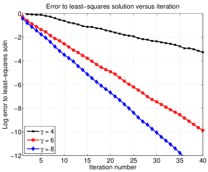
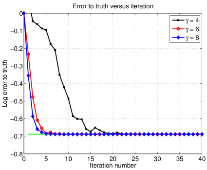
(a)	(b)

Figure 2: Simulations of the IHS algorithm for an unconstrained least-squares problem with noise variance $\sigma^{2}=1$, and of dimensions $(d,n)=(200,6000)$. Simulations based on sketch sizes $m=\gamma d$, for a parameter $\gamma>0$ to be set. (a) Plots of the log error $\|x^{t}-x^{\mbox{\tiny{LS}}}\|_{A}$ versus the iteration number $t$. Three different curves for $\gamma\in\{4,6,8\}$. Consistent with the theory, the convergence is geometric, with the rate increasing as the sampling factor $\gamma$ is increased. (b) Plots of the log error $\|x^{t}-x^{*}\|_{A}$ versus the iteration number $t$. Three different curves for $\gamma\in\{4,6,8\}$. As expected, all three curves flatten out at the level of the least-squares error $\|x^{\mbox{\tiny{LS}}}-x^{*}\|_{A}=0.20\approx\sqrt{\sigma^{2}d/n}$.

Assuming that the sketch dimension has been chosen to ensure geometric convergence, Theorem 2 allows us to specify, for a given target accuracy $\varepsilon\in(0,1)$, the number of iterations required.

Corollary 1.

Fix some $\rho\in(0,1/2)$, and choose a sketch dimension $m>\frac{c_{0}\log^{4}(D)}{\rho^{2}}\mathcal{W}^{2}(\mathcal{K}^{\mbox{\tiny{LS}}})$. If we apply the IHS algorithm for ${N}(\rho,\varepsilon):\,=1+\frac{\log(1/\varepsilon)}{\log(1/\rho)}$ steps, then the output $\widehat{x}=x^{{N}}$ satisfies the bound

$$\frac{\|\widehat{x}-x^{\mbox{\tiny{LS}}}\|_{A}}{\|x^{\mbox{\tiny{LS}}}\|_{A}} \leq\varepsilon$$ (27)

with probability at least $1-c_{1}{N}(\rho,\varepsilon)e^{-c_{2}\frac{m\rho^{2}}{\log^{4}(D)}}$.

This corollary is an immediate consequence of Theorem 2 combined with Lemma 1, and it holds for both ROS and sub-Gaussian sketches. (In the latter case, the additional $\log(D)$ terms may be omitted.) Combined with bounds on the width function $\mathcal{W}(\mathcal{K}^{\mbox{\tiny{LS}}})$, it leads to a number of concrete consequences for different statistical models, as we illustrate in the following section.

One way to understand the improvement of the IHS algorithm over the classical sketch is as follows. Fix some error tolerance $\varepsilon\in(0,1)$. Disregarding logarithmic factors, our previous results [31] on the classical sketch then imply that a sketch size $m\succsim\varepsilon^{-2}\>\mathcal{W}^{2}(\mathcal{K}^{\mbox{\tiny{LS}}})$ is sufficient to produce a $\varepsilon$-accurate solution approximation. In contrast, Corollary 1 guarantees that a sketch size $m\succsim\log(1/\varepsilon)\;\mathcal{W}^{2}(\mathcal{K}^{\mbox{\tiny{LS}}})$ is sufficient. Thus, the benefit is the reduction from $\varepsilon^{-2}$ to $\log(1/\varepsilon)$ scaling of the required sketch size.

It is worth noting that in the absence of constraints, the least-squares problem reduces to solving a linear system, so that alternative approaches are available. For instance, one can use a randomized sketch to obtain a preconditioner, which can then be used within the conjugate gradient method. As shown in past work [34, 4], two-step methods of this type can lead to same reduction of $\varepsilon^{-2}$ dependence to $\log(1/\varepsilon)$. However, a method of this type is very specific to unconstrained least-squares, whereas the procedure described in this paper is generally applicable to least-squares over any compact, convex constraint set.

2.5 Computational and space complexity

Let us now make a few comments about the computational and space complexity of implementing the IHS algorithm using ROS sketches (e.g., such as those based on the fast Hadamard transform). For a given sketch size $m$, at iteration $t$, the IHS algorithm requires $\mathcal{O}(nd\log(m))$ basic operation for computing the data sketch $S^{t+1}A$ and also $\mathcal{O}(nd)$ operations to compute $A^{T}(y-Ax^{t})$. Consequently, if we run the algorithm for ${N}$ iterations, then the overall complexity is $\mathcal{O}\big{(}(nd\log(m)+C(m,d))\,{N}\big{)}$, where $C(m,d)$ is the complexity of solving the $m\times d$ dimensional problem in the update (24). The total space used scales as $\mathcal{O}(md)$.

If we want to obtain estimates with accuracy $\varepsilon$, then we need to perform $N\asymp\log(1/\varepsilon)$ iterations in total. Moreover, for ROS sketches, we need to choose $m\succsim\mathcal{W}^{2}(\mathcal{K}^{\mbox{\tiny{LS}}})\log^{4}(d)$. Consequently, it only remains to bound the Gaussian width $\mathcal{W}$ in order to specify complexities that depend only on the pair $(n,d)$.

Unconstrained least-squares:

For an unconstrained problem with $n>d$, the Gaussian width can be bounded as $\mathcal{W}^{2}(\mathcal{K}^{\mbox{\tiny{LS}}})\precsim d$, and the complexity of the solving the sub-problem (24) can be bounded as $d^{3}$. Thus, the overall complexity of computing an $\varepsilon$-accurate solution scales as $\mathcal{O}(nd\log(d)+d^{3})\log(1/\varepsilon)$, and the space required is $\mathcal{O}(d^{2})$.

Sparse least-squares:

As will be shown in Section 3.2, in certain cases, the cone $\mathcal{K}^{\mbox{\tiny{LS}}}$ can have substantially lower complexity than the unconstrained case. For instance, if the solution is sparse, say with $s$ non-zero entries and the least-squares program involves an $\ell_{1}$-constraint, then we have $\mathcal{W}^{2}(\mathcal{K}^{\mbox{\tiny{LS}}})\precsim s\log d$. Using a standard interior point method to solve the sketched problem, the total complexity for obtaining an $\varepsilon$-accurate solution is upper bounded by $\mathcal{O}((nd\log(s)+s^{2}d\log^{2}(d))\log(1/\varepsilon))$, along with an $\mathcal{O}(sd\log(d))$ space complexity. The sparsity $s$ is not known a priori, however we note that there exists efficient bounds on $s$ which can be computed in $\mathcal{O}(nd)$ time (see e.g. [17]). Another approach is to impose some conditions on the design matrix $A$ which will guarantee support recovery, i.e., number of nonzero entries of $x^{*}$ equals $s$, (e.g., see [40]).

3 Consequences for concrete models

In this section, we derive some consequences of Corollary 1 for particular classes of least-squares problems. Our goal is to provide empirical confirmation of the sharpness of our theoretical predictions, namely the minimal sketch dimension required in order to match the accuracy of the original least-squares solution.

3.1 Unconstrained least squares

We begin with the simplest case, namely the unconstrained least-squares problem ($\mathcal{C}=\mathbb{R}^{d}$). For a given pair $(n,d)$ with $n>d$, we generated a random ensemble of least-square problems according to the following procedure:

• first, generate a random data matrix $A\in\mathbb{R}^{n\times d}$ with i.i.d. $N(0,1)$ entries

• second, choose a regression vector $x^{*}$ uniformly at random from the sphere $\mathcal{S}^{d-1}$

• third, form the response vector $y=Ax^{*}+w$, where $w\sim N(0,\sigma^{2}I_{n})$ is observation noise with $\sigma=1$.

As discussed following Lemma 1, for this class of problems, taking a sketch dimension $m\succsim\frac{d}{\rho^{2}}$ guarantees $\rho$-contractivity of the IHS iterates with high probability. Consequently, we can obtain a $\varepsilon$-accurate approximation to the original least-squares solution by running roughly $\log(1/\varepsilon)/\log(1/\rho)$ iterations.

Now how should the tolerance $\varepsilon$ be chosen? Recall that the underlying reason for solving the least-squares problem is to approximate $x^{*}$. Given this goal, it is natural to measure the approximation quality in terms of $\|x^{t}-x^{*}\|_{A}$. Panel (b) of Figure 2 shows the convergence of the iterates to $x^{*}$. As would be expected, this measure of error levels off at the ordinary least-squares error

$$\|x^{\mbox{\tiny{LS}}}-x^{*}\|_{A}^{2}\asymp\frac{\sigma^{2}d}{n}\approx 0.10.$$

Consequently, it is reasonable to set the tolerance parameter proportional to $\sigma^{2}\frac{d}{n}$, and then perform roughly $1+\frac{\log(1/\varepsilon)}{\log(1/\rho)}$ steps. The following corollary summarizes the properties of the resulting procedure:

Corollary 2.

For some given $\rho\in(0,1/2)$, suppose that we run the IHS algorithm for ${N}=1+\lceil\frac{\log\sqrt{n}\;\frac{\|x^{\mbox{\tiny{LS}}}\|_{A}}{\sigma}}{\log(1/\rho)}\rceil$ iterations using $m=\frac{c_{0}}{\rho^{2}}d$ projections per round. Then the output $\widehat{x}$ satisfies the bounds

$$\|\widehat{x}-x^{\mbox{\tiny{LS}}}\|_{A}\leq\sqrt{\frac{\sigma^{2}d}{n}},\qquad\mbox{and}\qquad\|x^{{N}}-x^{*}\|_{A}\leq\sqrt{\frac{\sigma^{2}d}{n}}+\|x^{\mbox{\tiny{LS}}}-x^{*}\|_{A}$$ (28)

with probability greater than $1-c_{1}\,{N}\,e^{-c_{2}\frac{m\rho^{2}}{\log^{4}(d)}}$.

In order to confirm the predicted bound (28) on the error $\|\widehat{x}-x^{\mbox{\tiny{LS}}}\|_{A}$, we performed a second experiment. Fixing $n=100d$, we generated $T=20$ random least squares problems from the ensemble described above with dimension $d$ ranging over $\{32,64,128,256,512\}$. By our previous choices, the least-squares estimate should have error $\|x^{\mbox{\tiny{LS}}}-x^{*}\|_{2}\approx\sqrt{\frac{\sigma^{2}d}{n}}=0.1$ with high probability, independently of the dimension $d$. This predicted behavior is confirmed by the blue bars in Figure 3; the bar height corresponds to the average over $T=20$ trials, with the standard errors also marked. On these same problem instances, we also ran the IHS algorithm using $m=6d$ samples per iteration, and for a total of

$${N} =1+\lceil\frac{\log\big{(}\sqrt{\frac{n}{d}}\big{)}}{\log 2}\rceil\;=4\qquad\mbox{iterations.}$$

Since $\|x^{\mbox{\tiny{LS}}}-x^{*}\|_{A}\asymp\sqrt{\frac{\sigma^{2}d}{n}}\approx 0.10$, Corollary 2 implies that with high probability, the sketched solution $\widehat{x}=x^{{N}}$ satisfies the error bound

$$\|\widehat{x}-x^{*}\|_{2} \leq c^{\prime}_{0}\;\sqrt{\frac{\sigma^{2}d}{n}}$$

for some constant $c^{\prime}_{0}>0$. This prediction is confirmed by the green bars in Figure 3, showing that $\|\widehat{x}-x^{*}\|_{A}\approx 0.11$ across all dimensions. Finally, the red bars show the results of running the classical sketch with a sketch dimension of $(6\times 4)d=24d$ sketches, corresponding to the total number of sketches used by the IHS algorithm. Note that the error is roughly twice as large.

Figure 3: Simulations of the IHS algorithm for unconstrained least-squares. In these experiments, we generated random least-squares problem of dimensions $d\in\{16,32,64,128,256\}$, on all occasions with a fixed sample size $n=100d$. The initial least-squares solution has error $\|x^{\mbox{\tiny{LS}}}-x^{*}\|_{A}\approx 0.10$, as shown by the blue bars. We then ran the IHS algorithm for ${N}=4$ iterations with a sketch size $m=6d$. As shown by the green bars, these sketched solutions show an error $\|\widehat{x}-x^{*}\|_{A}\approx 0.11$ independently of dimension, consistent with the predictions of Corollary 2. Finally, the red bars show the error in the classical sketch, based on a sketch size $M={N}m=24d$, corresponding to the total number of projections used in the iterative algorithm. This error is roughly twice as large.

3.2 Sparse least-squares

We now turn to a study of an $\ell_{1}$-constrained form of least-squares, referred to as the Lasso or relaxed basis pursuit [11, 37]. In particular, consider the convex program

$$x^{\mbox{\tiny{LS}}} =\arg\min_{\|x\|_{1}\leq R}\big{\{}\frac{1}{2}\|y-Ax\|_{2}^{2}\big{\}},$$ (29)

where $R>0$ is a user-defined radius. This estimator is well-suited to the problem of sparse linear regression, based on the observation model $y=Ax^{*}+w$, where $x^{*}$ has at most $s$ non-zero entries, and $A\in\mathbb{R}^{n\times d}$ has i.i.d. $N(0,1)$ entries. For the purposes of this illustration, we assume that the radius is chosen such that $R=\|x^{*}\|_{1}$.

Under these conditions, the proof of Corollary 3 shows that a sketch size $m\geq\gamma\,s\log\big{(}\frac{ed}{s}\big{)}$ suffices to guarantee geometric convergence of the IHS updates. Panel (a) of Figure 4 illustrates the accuracy of this prediction, showing the resulting convergence rate of the the IHS algorithm, measured in terms of the error $\|x^{t}-x^{\mbox{\tiny{LS}}}\|_{A}$, for different values $\gamma\in\{2,5,25\}$. As predicted by Theorem 2, the convergence rate is geometric (linear on the log scale shown), with the rate increasing as the parameter $\gamma$ is increased.

As long as $n\succsim s\log\big{(}\frac{ed}{s}\big{)}$, it also follows as a corollary of Proposition 2 that

$$\|x^{\mbox{\tiny{LS}}}-x^{*}\|_{A}^{2}\precsim\frac{\sigma^{2}s\log\big{(}\frac{ed}{s}\big{)}}{n}.$$ (30)

with high probability. This bound suggests an appropriate choice for the tolerance parameter $\varepsilon$ in Theorem 2, and leads us to the following guarantee.

Corollary 3.

For the stated random ensemble of sparse linear regression problems, suppose that we run the IHS algorithm for ${N}=1+\lceil\frac{\log\sqrt{n}\;\frac{\|x^{\mbox{\tiny{LS}}}\|_{A}}{\sigma}}{\log(1/\rho)}\rceil$ iterations using $m=\frac{c_{0}}{\rho^{2}}s\log\big{(}\frac{ed}{s}\big{)}$ projections per round. Then with probability greater than $1-c_{1}\,{N}\,e^{-c_{2}\frac{m\rho^{2}}{\log^{4}(d)}}$, the output $\widehat{x}$ satisfies the bounds

$$\|\widehat{x}-x^{\mbox{\tiny{LS}}}\|_{A}\leq\sqrt{\frac{\sigma^{2}s\log\big{(}\frac{ed}{s}\big{)}}{n}}\qquad\mbox{and}\qquad\|x^{{N}}-x^{*}\|_{A}\leq\sqrt{\frac{\sigma^{2}s\log\big{(}\frac{ed}{s}\big{)}}{n}}+\|x^{\mbox{\tiny{LS}}}-x^{*}\|_{A}.$$ (31)

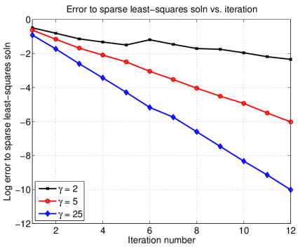
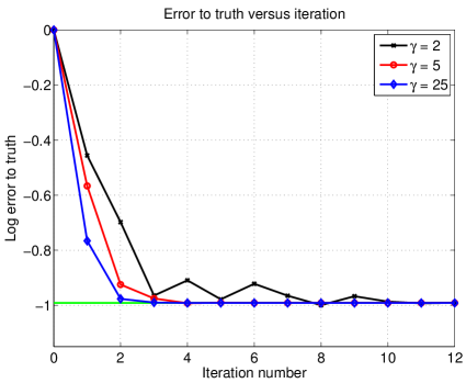
(a)	(b)

Figure 4: Simulations of the IHS algorithm for a sparse least-squares problem with noise variance $\sigma^{2}=1$, and of dimensions $(d,n,s)=(256,8872,32)$. Simulations based on sketch sizes $m=\gamma s\log d$, for a parameter $\gamma>0$ to be set. (a) Plots of the log error $\|x^{t}-x^{\mbox{\tiny{LS}}}\|_{2}$ versus the iteration number $t$. Three different curves for $\gamma\in\{2,5,25\}$. Consistent with the theory, the convergence is geometric, with the rate increasing as the sampling factor $\gamma$ is increased. (b) Plots of the log error $\|x^{t}-x^{*}\|_{2}$ versus the iteration number $t$. Three different curves for $\gamma\in\{2,5,25\}$. As expected, all three curves flatten out at the level of the least-squares error $\|x^{\mbox{\tiny{LS}}}-x^{*}\|_{2}=0.10\approx\sqrt{\frac{s\log(ed/s)}{n}}$.

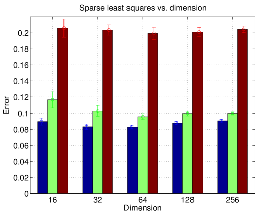
Figure 5: Simulations of the IHS algorithm for $\ell_{1}$-constrained least-squares. In these experiments, we generated random sparse least-squares problem of dimensions $d\in\{16,32,64,128,256\}$ and sparsity $s=\lceil 2\sqrt{d}\rceil$, on all occasions with a fixed sample size $n=100s\log\big{(}\frac{ed}{s}\big{)}$. The initial Lasso solution has error $\|x^{\mbox{\tiny{LS}}}-x^{*}\|_{2}\approx 0.10$, as shown by the blue bars. We then ran the IHS algorithm for ${N}=4$ iterations with a sketch size $m=4s\log\big{(}\frac{ed}{s}\big{)}$. These sketched solutions show an error $\|\widehat{x}-x^{*}\|_{A}\approx 0.11$ independently of dimension, consistent with the predictions of Corollary 3. Red bars show the error in the naive sketch estimate, using a sketch of size $M={N}m=16s\log\big{(}\frac{ed}{s}\big{)}$, equal to the total number of random projections used by the IHS algorithm. The resulting error is roughly twice as large.

In order to verify the predicted bound (31) on the error $\|\widehat{x}-x^{\mbox{\tiny{LS}}}\|_{A}$, we performed a second experiment. Fixing $n=100s\log\big{(}\frac{ed}{s}\big{)}$. we generated $T=20$ random least squares problems (as described above) with the regression dimension ranging as $d\in\{32,64,128,256\}$, and sparsity $s=\lceil 2\sqrt{d}\rceil$. Based on these choices, the least-squares estimate should have error $\|x^{\mbox{\tiny{LS}}}-x^{*}\|_{A}\approx\sqrt{\frac{\sigma^{2}s\log\big{(}\frac{ed}{s}\big{)}}{n}}=0.1$ with high probability, independently of the pair $(s,d)$. This predicted behavior is confirmed by the blue bars in Figure 5; the bar height corresponds to the average over $T=20$ trials, with the standard errors also marked.

On these same problem instances, we also ran the IHS algorithm using ${N}=4$ iterations with a sketch size $m=4s\log\big{(}\frac{ed}{s}\big{)}$. Together with our earlier calculation of $\|x^{\mbox{\tiny{LS}}}-x^{*}\|_{A}$, Corollary 2 implies that with high probability, the sketched solution $\widehat{x}=x^{{N}}$ satisfies the error bound

$$\|\widehat{x}-x^{*}\|_{A} \leq c_{0}\;\sqrt{\frac{\sigma^{2}s\log\big{(}\frac{ed}{s}\big{)}}{n}}$$

for some constant $c_{0}\in(1,2]$. This prediction is confirmed by the green bars in Figure 5, showing that $\|\widehat{x}-x^{*}\|_{A}\succsim 0.11$ across all dimensions. Finally, the green bars in Figure 5 show the error based on using the naive sketch estimate with a total of $M={N}m$ random projections in total; as with the case of ordinary least-squares, the resulting error is roughly twice as large. We also note that a similar bound also applies to problems where a parameter constrained to unit simplex is estimated, e.g., in portfolio analysis and density estimation [26, 30].

3.3 Matrix estimation with nuclear norm constraints

We now turn to the study of nuclear-norm constrained form of least-squares matrix regression. This class of problems has proven useful in many different application areas, among them matrix completion, collaborative filtering, multi-task learning and control theory (e.g., [18, 42, 5, 33, 28]). In particular, let us consider the convex program

$$X^{\mbox{\tiny{LS}}} =\arg\min_{X\in\mathbb{R}^{d_{1}\times d_{2}}}\Big{\{}\frac{1}{2}|\!|\!|Y-AX|\!|\!|_{{\mbox{\tiny{fro}}}}^{2}\Big{\}}\qquad\mbox{such that $|\!|\!|X|\!|\!|_{{\mbox{\tiny{nuc}}}}\leq R$,}$$ (32)

where $R>0$ is a user-defined radius as a regularization parameter.

3.3.1 Simulated data

Recall the linear observation model previously introduced in Example 3: we observe the pair $(Y,A)$ linked according to the linear $Y=AX^{*}+W$, where the unknown matrix $X^{*}\in\mathbb{R}^{d_{1}\times d_{2}}$ is an unknown matrix of rank $r$. The matrix $W$ is observation noise, formed with i.i.d. $N(0,\sigma^{2})$ entries. This model is a special case of the more general class of matrix regression problems [28]. As shown in Appendix D.2, if we solve the nuclear-norm constrained problem with $R=|\!|\!|X^{*}|\!|\!|_{{\mbox{\tiny{nuc}}}}$, then it produces a solution such that $\mathbb{E}\big{[}|\!|\!|X^{\mbox{\tiny{LS}}}-X^{*}|\!|\!|_{{\mbox{\tiny{fro}}}}^{2}]\precsim\sigma^{2}\frac{r\,(d_{1}+d_{2})}{n}$. The following corollary characterizes the sketch dimension and iteration number required for the IHS algorithm to match this scaling up to a constant factor.

Corollary 4 (IHS for nuclear-norm constrained least squares).

Suppose that we run the IHS algorithm for ${N}=1+\lceil\frac{\log\sqrt{n}\;\frac{\|X^{\mbox{\tiny{LS}}}\|_{A}}{\sigma}}{\log(1/\rho)}\rceil$ iterations using $m={c_{0}}{\rho^{2}}r\big{(}d_{1}+d_{2}\big{)}$ projections per round. Then with probability greater than $1-c_{1}\,{N}\,e^{-c_{2}\frac{m\rho^{2}}{\log^{4}(d_{1}d_{2})}}$, the output $X^{N}$ satisfies the bound

$$\|X^{{N}}-X^{*}\|_{A}\leq\sqrt{\frac{\sigma^{2}r\big{(}d_{1}+d_{2}\big{)}}{n}}+\|X^{\mbox{\tiny{LS}}}-X^{*}\|_{A}.$$ (33)

We have also performed simulations for low-rank matrix estimation, and observed that the IHS algorithm exhibits convergence behavior qualitatively similar to that shown in Figures 3 and 5. Similarly, panel (a) of Figure 7 compares the performance of the IHS and classical methods for sketching the optimal solution over a range of row sizes $n$. As with the unconstrained least-squares results from Figure 1, the classical sketch is very poor compared to the original solution whereas the IHS algorithm exhibits near optimal performance.

3.3.2 Application to multi-task learning

To conclude, let us illustrate the use of the IHS algorithm in speeding up the training of a classifier for facial expressions. In particular, suppose that our goal is to separate a collection of facial images into different groups, corresponding either to distinct individuals or to different facial expressions. One approach would be to learn a different linear classifier ($a\mapsto\langle a,\,x\rangle$) for each separate task, but since the classification problems are so closely related, the optimal classifiers are likely to share structure. One way of capturing this shared structure is by concatenating all the different linear classifiers into a matrix, and then estimating this matrix in conjunction with a nuclear norm penalty [2, 3].

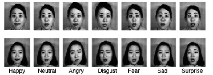
Figure 6: Japanese Female Facial Expression (JAFFE) Database: The JAFFE database consists of 213 images of 7 different emotional facial expressions (6 basic facial expressions + 1 neutral) posed by 10 Japanese female models.

In more detail, we performed a simulation study using the The Japanese Female Facial Expression (JAFFE) database [24]. It consists of $N=213$ images of $7$ facial expressions ($6$ basic facial expressions + $1$ neutral) posed by $10$ different Japanese female models; see Figure 6 for a few example images. We performed an approximately $80:20$ split of the data set into $n_{\mbox{\footnotesize{train}}}=170$ training and $n_{\mbox{\footnotesize{test}}}=43$ test images respectively. Then we consider classifying each facial expression and each female model as a separate task which gives a total of $d_{\mbox{\footnotesize{task}}}=17$ tasks. For each task $j=1,\ldots,d_{\mbox{\footnotesize{task}}}$, we construct a linear classifier of the form $a\mapsto\operatorname{sign}(\langle a,\,x_{j}\rangle)$, where $a\in\mathbb{R}^{d}$ denotes the vectorized image features given by Local Phase Quantization [29]. In our implementation, we fixed the number of features $d=32$. Given this set-up, we train the classifiers in a joint manner, by optimizing simultaneously over the matrix $X\in\mathbb{R}^{d\times d_{\mbox{\footnotesize{task}}}}$ with the classifier vector $x_{j}\in\mathbb{R}^{d}$ as its $j^{th}$ column. The image data is loaded into the matrix $A\in\mathbb{R}^{n_{\mbox{\footnotesize{train}}}\times d}$, with image feature vector $a_{i}\in\mathbb{R}^{d}$ in column $i$ for $i=1,\ldots,n_{\mbox{\footnotesize{train}}}$. Finally, the matrix $Y\in\{-1,+1\}^{n_{\mbox{\footnotesize{train}}}\times d_{\mbox{\footnotesize{task}}}}$ encodes class labels for the different classification problems. These instantiations of the pair $(Y,X)$ give us an optimization problem of the form (32), and we solve it over a range of regularization radii $R$.

More specifically, in order to verify the classification accuracy of the classifier obtained by IHT algorithm, we solved the original convex program, the classical sketch based on ROS sketches of dimension $m=100$, and also the corresponding IHS algorithm using ROS sketches of size $20$ in each of $5$ iterations. In this way, both the classical and IHS procedures use the same total number of sketches, making for a fair comparison. We repeated each of these three procedures for all choices of the radius $R\in\{1,2,3,\ldots,12\}$, and then applied the resulting classifiers to classify images in the test dataset. For each of the three procedures, we calculated the classification error rate, defined as the total number of mis-classified images divided by $n_{\mbox{\footnotesize{test}}}\times d_{\mbox{\footnotesize{task}}}$. Panel (b) of Figure 7 plots the resulting classification errors versus the regularization parameter. The error bars correspond to one standard deviation calculated over the randomness in generating sketching matrices. The plots show that the IHS algorithm yields classifiers with performance close to that given by the original solution over a range of regularizer parameters, and is superior to the classification sketch. The error bars also show that the IHS algorithm has less variability in its outputs than the classical sketch.

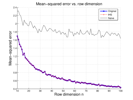
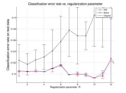
(a)	(b)

Figure 7: Simulations of the IHS algorithm for nuclear-norm constrained problems. The blue curves correspond to the solution of the original (unsketched problem), wheras red curves correspond to the IHS method applied for ${N}=1+\lceil\log(n)\rceil$ rounds using a sketch size of $m$. Black curves correpsond to the naive sketch applied using $M=Nm$ projections in total, corresponding to the same number used in all iterations of the IHS algorithm. (a) Mean-squared error versus the row dimension $n\in[10,100]$ for recovering a $20\times 20$ matrix of rank $r2$, using a sketch dimension $m=60$. Note how the accuracy of the IHS algorithm tracks the error of the unsketched solution over a wide range of $n$, whereas the classical sketch has essentially constant error. (b) Classification error rate versus regularization parameter $R\in\{1,\ldots,12\}$, with error bars corresponding to one standard deviation over the test set. Sketching algorithms were applied to the JAFFE face expression using a sketch dimension of $M=100$ for the classical sketch, and $N=5$ iterations with $m=20$ sketches per iteration for the IHS algorithm.

4 Discussion

In this paper, we focused on the problem of solution approximation (as opposed to cost approximation) for a broad class of constrained least-squares problem. We began by showing that the classical sketching methods are sub-optimal, from an information-theoretic point of view, for the purposes of solution approximation. We then proposed a novel iterative scheme, known as the iterative Hessian sketch, for deriving $\varepsilon$-accurate solution approximations. We proved a general theorem on the properties of this algorithm, showing that the sketch dimension per iteration need grow only proportionally to the statistical dimension of the optimal solution, as measured by the Gaussian width of the tangent cone at the optimum. By taking $\log(1/\varepsilon)$ iterations, the IHS algorithm is guaranteed to return an $\varepsilon$-accurate solution approximation with exponentially high probability.

In addition to these theoretical results, we also provided empirical evaluations that reveal the sub-optimality of the classical sketch, and show that the IHS algorithm produces near-optimal estimators. Finally, we applied our methods to a problem of facial expression using a multi-task learning model applied to the JAFFE face database. We showed that IHS algorithm applied to a nuclear-norm constrained program produces classifiers with considerably better classification accuracy compared to the naive sketch.

There are many directions for further research, but we only list here some of them. The idea behind iterative sketching can also be applied to problems beyond minimizing a least-squares objective function subject to convex constraints. An important class of such problems are $\ell_{p}$-norm forms of regression, based on the convex program

$$\min_{x\in\mathbb{R}^{d}}\|Ax-y\|_{p}^{p}\qquad\mbox{for some $p\in[1,\infty]$.}$$

The case of $\ell_{1}$-regression ($p=1$) is an important special case, known as robust regression; it is especially effective for data sets containing outliers [20]. Recent work [12] has proposed to find faster solutions of the $\ell_{1}$-regression problem using the classical sketch (i.e., based on $(SA,Sy)$) but with sketching matrices based on Cauchy random vectors. Based on the results of the current paper, our iterative technique might be useful in obtaining sharper bounds for solution approximation in this setting as well.

Acknowledgements

Both authors were partially supported by Office of Naval Research MURI grant N00014-11-1-0688, and National Science Foundation Grants CIF-31712-23800 and DMS-1107000. In addition, MP was supported by a Microsoft Research Fellowship.

Appendix A Proof of lower bounds

This appendix is devoted to the verification of condition (9) for different model classes, followed by the proof of Theorem 1.

A.1 Verification of condition (9)

We verify the condition for three different types of sketches.

Gaussian sketches:

First, let $S\in\mathbb{R}^{m\times n}$ be a random matrix with i.i.d. Gaussian entries. We use the singular value decomposition to write $S=U\Lambda V^{T}$ where both $U$ and $V$ are orthonormal matrices of left and right singular vectors. By rotation invariance, the columns $\{v_{i}\}_{i=1}^{m}$ are uniformly distributed over the sphere $\mathcal{S}^{n-1}$. Consquently, we have

$$\mathbb{E}_{S}\big{[}S^{T}\big{(}SS^{T})^{-1}S\big{]} =\mathbb{E}\sum_{i=1}^{m}v_{i}v_{i}^{T}=\frac{m}{n}I_{n},$$ (34)

showing that condition (9) holds with $\eta=1$.

ROS sketches:

In this case, we have $S=\sqrt{n}PHD$, where $P\in\mathbb{R}^{m\times n}$ is a random picking matrix (with each row being a standard basis vector). We then have $SS^{T}=nI_{m}$ and also $\mathbb{E}_{P}[P^{T}P]=\frac{m}{n}I_{n}$, so that

$$\mathbb{E}_{S}[S^{T}(SS^{T})^{-1}S] =\mathbb{E}_{D,P}[DH^{T}P^{T}PHD]=\mathbb{E}_{D}[DH^{T}(\frac{m}{n}I_{n})HD]=\frac{m}{n}I_{n},$$

showing that the condition holds with $\eta=1$.

Weighted row sampling:

Finally, suppose that we sample $m$ rows independently using a distribution $\{p_{j}\}_{j=1}^{n}$ on the rows of the data matrix that is $\alpha$-balanced (7). Letting $\mathcal{R}\subseteq\{1,2,\ldots,n\}$ be the subset of rows that are sampled, and let $N_{j}$ be the number of times each row is sampled. We then have

$$\mathbb{E}\Big{[}S^{T}\big{(}SS^{T})^{-1}S\Big{]} =\sum_{j\in\mathcal{R}}\mathbb{E}[e_{j}e_{j}^{T}]\;=\;D,$$

where $D\in\mathbb{R}^{n\times n}$ is a diagonal matrix with entries $D_{jj}=\mathbb{P}[j\in\mathcal{R}]$. Since the trials are independent, the $j^{th}$ row is sampled at least once in $m$ trials with probability $q_{j}=1-(1-p_{j})^{m}$, and hence

$$\mathbb{E}_{S}\big{[}S^{T}\big{(}SS^{T})^{-1}S\big{]} =\operatorname{diag}\big{(}\{1-(1-p_{i})^{m}\}_{i=1}^{m}\big{)}\;\preceq\;\big{(}1-(1-p_{\infty})^{m}\big{)}I_{n}\;\preceq mp_{\infty},$$

where $p_{\infty}=\max_{j\in[n]}p_{j}$. Consequently, as long as the row weights are $\alpha$-balanced (7) so that $p_{\infty}\leq\frac{\alpha}{n}$, we have

$$|\!|\!|\mathbb{E}_{S}\big{[}S^{T}\big{(}SS^{T})^{-1}S\big{]}|\!|\!|_{{\mbox{\tiny{op}}}} \leq\alpha\frac{m}{n}$$

showing that condition (9) holds with $\eta=\alpha$, as claimed.

A.2 Proof of Theorem 1

Let $\{z^{j}\}_{j=1}^{M}$ be a $1/2$-packing of $\mathcal{C}_{0}$ in the semi-norm $\|\cdot\|_{A}$ and for a fixed $\delta\in(0,1/4)$, define $x^{j}=4\delta z^{j}$. We thus obtain a collection of vectors in $\mathcal{C}_{0}$ such that

$$2\delta\leq\frac{1}{\sqrt{n}}\|A(x^{j}-x^{k})\|_{2}\leq 8\delta\qquad\mbox{for all $j\neq k$.}$$

Letting $J$ be a random index uniformly distributed over $\{1,\ldots,M\}$, suppose that conditionally on $J=j$, we observe the sketched observation vector $Sy=SAx^{j}+Sw$, as well as the sketched matrix $SA$. Conditioned on $J=j$, the random vector $Sy$ follows a $\mathcal{N}(SAx^{j},\sigma^{2}SS^{T})$ distribution, denoted by $\mathbb{P}_{x^{j}}$. We let $\makebox[0.0pt][l]{\hskip 2.05pt\rule[8.12498pt]{5.67886pt}{0.43057pt}}{Y}$ denote the resulting mixture variable, with distribution $\frac{1}{M}\sum_{j=1}^{M}\mathbb{P}_{x^{j}}$.

Consider the multiway testing problem of determining the index $J$ based on observing $\makebox[0.0pt][l]{\hskip 2.05pt\rule[8.12498pt]{5.67886pt}{0.43057pt}}{Y}$. With this set-up, a standard reduction in statistical minimax (e.g., [7, 41]) implies that, for any estimator $x^{\dagger}$, the worst-case mean-squared error is lower bounded as

$$\sup_{x^{*}\in\mathcal{C}}\mathbb{E}_{S,w}\|x^{\dagger}-x^{*}\|_{A}^{2} \geq\delta^{2}\inf_{\psi}\mathbb{P}[\psi(\makebox[0.0pt][l]{\hskip 2.05pt\rule[8.12498pt]{5.67886pt}{0.43057pt}}{Y})\neq J],$$ (35)

where the infimum ranges over all testing functions $\psi$. Consequently, it suffices to show that the testing error is lower bounded by $1/2$.

In order to do so, we first apply Fano’s inequality [13] conditionally on the sketching matrix $S$ to see that

$$\mathbb{P}[\psi(\makebox[0.0pt][l]{\hskip 2.05pt\rule[8.12498pt]{5.67886pt}{0.43057pt}}{Y})\neq J]\;=\;\mathbb{E}_{S}\Big{\{}\mathbb{P}[\psi(\makebox[0.0pt][l]{\hskip 2.05pt\rule[8.12498pt]{5.67886pt}{0.43057pt}}{Y})\neq J\mid S]\Big{\}} \geq 1-\frac{\mathbb{E}_{S}\big{[}I_{S}(\makebox[0.0pt][l]{\hskip 2.05pt\rule[8.12498pt]{5.67886pt}{0.43057pt}}{Y};J)\big{]}+\log 2}{\log M},$$ (36)

where $I_{S}(\makebox[0.0pt][l]{\hskip 2.05pt\rule[8.12498pt]{5.67886pt}{0.43057pt}}{Y};J)$ denotes the mutual information between $\makebox[0.0pt][l]{\hskip 2.05pt\rule[8.12498pt]{5.67886pt}{0.43057pt}}{Y}$ and $J$ with $S$ fixed. Our next step is to upper bound the expectation $\mathbb{E}_{S}[I(\makebox[0.0pt][l]{\hskip 2.05pt\rule[8.12498pt]{5.67886pt}{0.43057pt}}{Y};J)]$.

Letting $D(\mathbb{P}_{x^{j}}\;\|\;\mathbb{P}_{x^{k}})$ denote the Kullback-Leibler divergence between the distributions $\mathbb{P}_{x^{j}}$ and $\mathbb{P}_{x^{k}}$, the convexity of Kullback-Leibler divergence implies that

$$I_{S}(\makebox[0.0pt][l]{\hskip 2.05pt\rule[8.12498pt]{5.67886pt}{0.43057pt}}{Y};J) =\frac{1}{M}\sum_{j=1}^{M}D(\mathbb{P}_{x^{j}}\;\|\;\frac{1}{M}\sum_{k=1}^{M}\mathbb{P}_{x^{k}})\;\leq\;\frac{1}{M^{2}}\sum_{j,k=1}^{M}D(\mathbb{P}_{x^{j}}\;\|\;\mathbb{P}_{x^{k}}).$$

Computing the KL divergence for Gaussian vectors yields

$$I_{S}(\makebox[0.0pt][l]{\hskip 2.05pt\rule[8.12498pt]{5.67886pt}{0.43057pt}}{Y};J) \leq\frac{1}{M^{2}}\sum_{j,k=1}^{M}\frac{1}{2\sigma^{2}}(x^{j}-x^{k})^{T}A^{T}\Big{[}S^{T}(SS^{T})^{-1}S\Big{]}A(x^{j}-x^{k}).$$

Thus, using condition (9), we have

$$\mathbb{E}_{S}[I(\makebox[0.0pt][l]{\hskip 2.05pt\rule[8.12498pt]{5.67886pt}{0.43057pt}}{Y};J)] \leq\frac{1}{M^{2}}\sum_{j,k=1}^{M}\frac{m\;\eta}{2\,n\sigma^{2}}\|A(x^{j}-x^{k})\|_{2}^{2}\;\leq\frac{32\,m\,\eta}{\sigma^{2}}\,\delta^{2},$$

where the final inequality uses the fact that $\|x^{j}-x^{k}\|_{A}\leq 8\delta$ for all pairs.

Combined with our previous bounds (35) and (36), we find that

$$\sup_{x^{*}\in\mathcal{C}}\mathbb{E}\|\widehat{x}-x^{*}\|_{2}^{2} \geq\delta^{2}\Big{\{}1-\frac{32\frac{m\,\eta\,\delta^{2}}{\sigma^{2}}+\log 2}{\log M}\Big{\}}.$$

Setting $\delta=\frac{\sigma^{2}\log(M/2)}{64\,\eta\,m}$ yields the lower bound (10).

Appendix B Proof of Proposition 1

Since $\widehat{x}$ and $x^{\mbox{\tiny{LS}}}$ are optimal and feasible, respectively, for the Hessian sketch program (16), we have

$$\langle A^{T}S^{T}\big{(}SA\widehat{x}-y\big{)},\,x^{\mbox{\tiny{LS}}}-\widehat{x}\rangle \geq 0$$ (37a)

Similarly, since $$x^{\mbox{\tiny{LS}}} \widehat{x}$$ and are optimal and feasible, respectively, for the original least squares program

$$\langle A^{T}(Ax^{\mbox{\tiny{LS}}}-y),\,\widehat{x}-x^{\mbox{\tiny{LS}}}\rangle \geq 0.$$ (37b)

Adding these two inequalities and performing some algebra yields the basic inequality

$$\frac{1}{m}\|SA\Delta\|_{2}^{2} \leq\Big{|}(Ax^{\mbox{\tiny{LS}}})^{T}\big{(}I_{n}-\frac{S^{T}S}{m}\big{)}A\Delta\Big{|}.$$ (38)

Since $Ax^{\mbox{\tiny{LS}}}$ is independent of the sketching matrix and $A\Delta\in\mathcal{K}^{\mbox{\tiny{LS}}}$, we have

$$\frac{1}{m}\|SA\Delta\|_{2}^{2}\geq Z_{1}\,\|A\Delta\|_{2}^{2},\qquad\mbox{and}\quad\Big{|}(Ax^{\mbox{\tiny{LS}}})^{T}\big{(}I_{n}-S^{T}S\big{)}A\Delta\Big{|}\leq Z_{2}\|Ax^{\mbox{\tiny{LS}}}\|_{2}\,\|A\Delta\|_{2},$$

using the definitions (18a) and (18b) of the random variables $Z_{1}$ and $Z_{2}$ respectively. Combining the pieces yields the claim.

Appendix C Proof of Theorem 2

It suffices to show that, for each iteration $t=0,1,2,\ldots$, we have

$$\|x^{t+1}-x^{\mbox{\tiny{LS}}}\|_{A} \leq\frac{Z_{2}(S^{t+1})}{Z_{1}(S^{t+1})}\|x^{t}-x^{\mbox{\tiny{LS}}}\|_{A}.$$ (39)

The claimed bounds (26a) and  (26b) then follow by applying the bound (39) successively to iterates $1$ through ${N}$.

For simplicity in notation, we abbreviate $S^{t+1}$ to $S$ and $x^{t+1}$ to $\widehat{x}$. Define the error vector $\Delta=\widehat{x}-x^{\mbox{\tiny{LS}}}$. With some simple algebra, the optimization problem (24) that underlies the update $t+1$ can be re-written as

$$\widehat{x} =\arg\min_{x\in\mathcal{C}}\Big{\{}\frac{1}{2m}\|SAx\|_{2}^{2}-\langle A^{T}\widetilde{y},\,x\rangle\Big{\}},$$

where $\widetilde{y}:\,=y+\Big{[}I-\frac{S^{T}S}{m}\Big{]}Ax^{t}$. Since $\widehat{x}$ and $x^{\mbox{\tiny{LS}}}$ are optimal and feasible respectively, the usual first-order optimality conditions imply that

$$\langle A^{T}\frac{S^{T}S}{m}Ax-A^{T}\widetilde{y},\,x^{\mbox{\tiny{LS}}}-\widehat{x}\rangle \geq 0.$$

As before, since $x^{\mbox{\tiny{LS}}}$ is optimal for the original program, we have

$$\langle A^{T}(Ax^{\mbox{\tiny{LS}}}-\widetilde{y}+\Big{[}I-\frac{S^{T}S}{m}\Big{]}Ax^{t}),\,\widehat{x}-x^{\mbox{\tiny{LS}}}\rangle \geq 0.$$

Adding together these two inequalities and introducing the shorthand $\Delta=\widehat{x}-x^{\mbox{\tiny{LS}}}$ yields

$$\frac{1}{m}\|SA\Delta\|_{2}^{2} \leq\Big{|}(A(x^{\mbox{\tiny{LS}}}-x^{t})^{T}\big{[}I-\frac{S^{T}S}{m}\big{]}A\Delta\Big{|}$$ (40)

Note that the vector $A(x^{\mbox{\tiny{LS}}}-x^{t})$ is independent of the randomness in the sketch matrix $S^{t+1}$. Moreover, the vector $A\Delta$ belongs to the cone $\mathcal{K}$, so that by the definition of $Z_{2}(S^{t+1})$, we have

$$\Big{|}(A(x^{\mbox{\tiny{LS}}}-x^{t})^{T}\Big{[}I-\frac{S^{T}S}{m}\Big{]}A\Delta\Big{|} \leq\|A(x^{\mbox{\tiny{LS}}}-x^{t})\|_{2}\;\|A\Delta\|_{2}\;Z_{2}(S^{t+1}).$$ (41a)

Similarly, note the lower bound

$$\frac{1}{m}\|SA\Delta\|_{2}^{2} \geq\|A\Delta\|_{2}^{2}\;Z_{1}(S^{t+1}).$$ (41b)

Combining the two bounds (41a) and (41b) with the earlier bound (40) yields the claim (39).

Appendix D Maximum likelihood estimator and examples

In this section, we a general upper bound on the error of the constrained least-squares estimate. We then use it (and other results) to work through the calculations underlying Examples 1 through 3 from Section 2.2.

D.1 Upper bound on MLE

The accuracy of $x^{\mbox{\tiny{LS}}}$ as an estimate of $x^{*}$ depends on the “size” of the star-shaped set

$$\mathcal{K}(x^{*}) =\big{\{}v\in\mathbb{R}^{d}\,\mid v=\frac{t}{\sqrt{n}}\,A(x-x^{*})\quad\mbox{for some $t\in[0,1]$ and $x\in\mathcal{C}$}\big{\}}.$$ (42)

When the vector $x^{*}$ is clear from context, we use the shorthand notation $\mathcal{K}^{*}$ for this set. By taking a union over all possible $x^{*}\in\mathcal{C}_{0}$, we obtain the set $\makebox[0.0pt][l]{\hskip 2.05pt\rule[8.12498pt]{5.44139pt}{0.43057pt}}{\mathcal{K}}:\,=\bigcup\limits_{x^{*}\in\mathcal{C}_{0}}\mathcal{K}(x^{*})$, which plays an important role in our bounds. The complexity of these sets can be measured of their localized Gaussian widths. For any radius $\varepsilon>0$ and set $\Theta\subseteq\mathbb{R}^{n}$, the Gaussian width of the set $\Theta\cap\mathbb{B}_{2}(\varepsilon)$ is given by

$$\mathcal{W}_{\varepsilon}(\Theta) :\,=\mathbb{E}_{g}\Big{[}\sup_{\begin{subarray}{c}\theta\in\Theta\\ \|\theta\|_{2}\leq\varepsilon\end{subarray}}|\langle w,\,\theta\rangle|\Big{]},$$ (43a)

where $$g\sim N(0,I_{n\times n}) \Theta \sigma>0 \ell$$ is a standard Gaussian vector. Whenever the set is star-shaped, then it can be shown that, for any and positive integer , the inequality

$$\frac{\mathcal{W}_{\varepsilon}(\Theta)}{\varepsilon\,\sqrt{\ell}} \leq\frac{\varepsilon}{\sigma}$$ (43b)

has a smallest positive solution, which we denote by $\varepsilon_{\ell}(\Theta;\sigma)$. We refer the reader to Bartlett et al. [6] for further discussion of such localized complexity measures and their properties.

The following result bounds the mean-squared error associated with the constrained least-squares estimate:

Proposition 2.

For any set $\mathcal{C}$ containing $x^{*}$, the constrained least-squares estimate (1) has mean-squared error upper bounded as

$$\mathbb{E}_{w}\big{[}\|x^{\mbox{\tiny{LS}}}-x^{*}\|_{A}^{2}\big{]} \leq c_{1}\big{\{}\varepsilon_{n}^{2}\big{(}\mathcal{K}^{*}\big{)}+\frac{\sigma^{2}}{n}\big{\}}\;\leq\;c_{1}\big{\{}\varepsilon_{n}^{2}\big{(}\makebox[0.0pt][l]{\hskip 2.05pt\rule[8.12498pt]{5.44139pt}{0.43057pt}}{\mathcal{K}}\big{)}+\frac{\sigma^{2}}{n}\big{\}}.$$ (44)

We provide the proof of this claim in Section D.3.

D.2 Detailed calculations for illustrative examples

In this appendix, we collect together the details of calculations used in our illustrative examples from Section 2.2. In all cases, we make use tof the convenient shorthand $\widetilde{A}=A/\sqrt{n}$.

D.2.1 Unconstrained least squares: Example 1

By definition of the Gaussian width, we have

$$\mathcal{W}_{\delta}(\mathcal{K}^{*}) =\mathbb{E}_{g}\big{[}\sup_{\|\widetilde{A}\,(x-x^{*})\|_{2}\leq\delta}|\langle g,\,\widetilde{A}(x-x^{*})\rangle|\big{]}\;\leq\;\delta\,\sqrt{d}$$

since the vector $\widetilde{A}(x-x^{*})$ belongs to a subspace of dimension $\operatorname{rank}(A)=d$. The claimed upper bound (11a) thus follows as a consequence of Proposition 2.

D.2.2 Sparse vectors: Example 2

The RIP property of order $8s$ implies that

$$\frac{\|\Delta\|_{2}^{2}}{2}\;\stackrel{{\scriptstyle(i)}}{{\leq}}\|\widetilde{A}\Delta\|_{2}^{2}\;\stackrel{{\scriptstyle(ii)}}{{\leq}}\;2\|\Delta\|_{2}^{2}\qquad\mbox{for all vectors with $\|\Delta\|_{0}\leq 8s$,}$$

a fact which we use throughout the proof. By definition of the Gaussian width, we have

$$\mathcal{W}_{\delta}(\mathcal{K}^{*}) =\mathbb{E}_{g}\big{[}\sup_{\begin{subarray}{c}\|x\|_{1}\leq\|x^{*}\|_{1}\\ \|\widetilde{A}(x-x^{*})\|_{2}\leq\delta\end{subarray}}|\langle g,\,\widetilde{A}(x-x^{*})\rangle|\big{]}.$$

Since $x^{*}\in\mathbb{B}_{0}(s)$, it can be shown (e.g., see the proof of Corollary 3 in the paper [31]) that for any vector $\|x\|_{1}\leq\|x^{*}\|_{1}$, we have $\|x-x^{*}\|_{1}\leq 2\sqrt{s}\|x-x^{*}\|_{2}$. Thus, it suffices to bound the quantity

$$F(\delta;s) :\,=\mathbb{E}_{g}\big{[}\sup_{\begin{subarray}{c}\|\Delta\|_{1}\leq 2\sqrt{s}\|\Delta\|_{2}\\ \|\widetilde{A}\Delta\|_{2}\leq\delta\end{subarray}}|\langle g,\,\widetilde{A}\Delta\rangle|\big{]}.$$

By Lemma 11 in the paper [23], we have $\mathbb{B}_{1}(\sqrt{s})\cap\mathbb{B}_{2}(1)\subseteq 3\operatorname{clconv}\Big{\{}\mathbb{B}_{0}(s)\cap\mathbb{B}_{2}(1)\Big{\}}$, where $\operatorname{clconv}$ denotes the closed convex hull. Applying this lemma with $s=4s$, we have

$$F(\delta;s) \leq 3\big{[}\sup_{\begin{subarray}{c}\|\Delta\|_{0}\leq 4s\\ \|\widetilde{A}\Delta\|_{2}\leq\delta\end{subarray}}|\langle g,\,\widetilde{A}\Delta\rangle|\big{]}\;\leq\;3\mathbb{E}\big{[}\sup_{\begin{subarray}{c}\|\Delta\|_{0}\leq 4s\\ \|\Delta\|_{2}\leq 2\delta\end{subarray}}|\langle g,\,\widetilde{A}\Delta\rangle|\big{]},$$

using the lower RIP property (i). By the upper RIP property, for any pair of vectors $\Delta,\Delta^{\prime}$ with $\ell_{0}$-norms at most $4s$, we have

$$\operatorname{var}\big{(}\langle g,\,\widetilde{A}\Delta\rangle-\langle g,\,\widetilde{A}\Delta^{\prime}\rangle\big{)} \leq 2\|\Delta-\Delta^{\prime}\|_{2}^{2}\;=\;2\operatorname{var}\big{(}\langle g,\,\Delta-\Delta^{\prime}\rangle\big{)}$$

Consequently, by the Sudakov-Fernique comparison [22], we have

$$\mathbb{E}\big{[}\sup_{\begin{subarray}{c}\|\Delta\|_{0}\leq 4s\\ \|\Delta\|_{2}\leq 2\delta\end{subarray}}|\langle g,\,\widetilde{A}\Delta\rangle|\big{]} \leq 2\mathbb{E}\big{[}\sup_{\begin{subarray}{c}\|\Delta\|_{0}\leq 4s\\ \|\Delta\|_{2}\leq 2\delta\end{subarray}}|\langle g,\,\Delta\rangle|\big{]}\;\leq c\;\delta\sqrt{s\log\big{(}\frac{ed}{s}\big{)}},$$

where the final inequality standard results on Gaussian widths [19]. All together, we conclude that

$$\varepsilon_{n}^{2}(\mathcal{K}^{*};\sigma) \leq c_{1}\sigma^{2}\frac{s\log\big{(}\frac{ed}{s}\big{)}}{n}.$$

Combined with Proposition 2, the claimed upper bound (12a) follows.

In the other direction, a straightforward argument (e.g., [32]) shows that there is a universal constant $c>0$ such that $\log M_{1/2}\geq c\,s\log\big{(}\frac{ed}{s}\big{)}$, so that the stated lower bound follows from Theorem 1.

D.2.3 Low rank matrices: Example 3:

By definition of the Gaussian width, we have width, we have

$$\mathcal{W}_{\delta}(\mathcal{K}^{*}) =\mathbb{E}_{g}\Biggr{[}\sup_{\begin{subarray}{c}|\!|\!|\widetilde{A}\,(X-X^{*})|\!|\!|_{{\mbox{\tiny{fro}}}}\leq\delta\\ |\!|\!|X|\!|\!|_{{\mbox{\tiny{nuc}}}}\leq|\!|\!|X^{*}|\!|\!|_{{\mbox{\tiny{nuc}}}}\end{subarray}}|\langle\!\langle{\widetilde{A}^{T}G},\;{(X-X^{*})}\rangle\!\rangle|\Biggr{]},$$

where $G\in\mathbb{R}^{n\times d_{2}}$ is a Gaussian random matrix, and $\langle\!\langle{C},\;{D}\rangle\!\rangle$ denotes the trace inner product between matrices $C$ and $D$. Since $X^{*}$ has rank at most $r$, it can be shown that $|\!|\!|X-X^{*}|\!|\!|_{{\mbox{\tiny{nuc}}}}\leq 2\sqrt{r}|\!|\!|X-X^{*}|\!|\!|_{{\mbox{\tiny{fro}}}}$; for instance, see Lemma 1 in the paper [27]. Recalling that $\gamma_{\operatorname{\tiny{min}}}(\widetilde{A})$ denotes the minimum singular value, we have

$$|\!|\!|X-X^{*}|\!|\!|_{{\mbox{\tiny{fro}}}}\leq\frac{1}{\gamma_{\operatorname{\tiny{min}}}(\widetilde{A})}\,|\!|\!|\widetilde{A}(X-X^{*})|\!|\!|_{{\mbox{\tiny{fro}}}}\leq\frac{\delta}{\gamma_{\operatorname{\tiny{min}}}(\widetilde{A})}.$$

Thus, by duality between the nuclear and operator norms, we have

$$\mathbb{E}_{g}\Biggr{[}\sup_{\begin{subarray}{c}|\!|\!|\widetilde{A}\,(X-X^{*})|\!|\!|_{{\mbox{\tiny{fro}}}}\leq\delta\\ |\!|\!|X|\!|\!|_{{\mbox{\tiny{nuc}}}}\leq|\!|\!|X^{*}|\!|\!|_{{\mbox{\tiny{nuc}}}}\end{subarray}}|\langle\!\langle{G},\;{\widetilde{A}(X-X^{*})}\rangle\!\rangle|\Biggr{]} \leq\frac{2\,\sqrt{r}\,\delta}{\gamma_{\operatorname{\tiny{min}}}(A)}\,\mathbb{E}\big{[}|\!|\!|\widetilde{A}^{T}G|\!|\!|_{{\mbox{\tiny{op}}}}].$$

Now consider the matrix $A^{T}G\in\mathbb{R}^{d_{1}\times d_{2}}$. For any fixed pair of vectors $(u,v)\in\mathcal{S}^{d_{1}-1}\times\mathcal{S}^{d_{2}-1}$, the random variable $Z=u^{T}\widetilde{A}^{T}Gv$ is zero-mean Gaussian with variance at most $\gamma_{\operatorname{\tiny{max}}}^{2}(\widetilde{A})$. Consequently, by a standard covering argument in random matrix theory [39], we have $\mathbb{E}\big{[}|\!|\!|\widetilde{A}^{T}G|\!|\!|_{{\mbox{\tiny{op}}}}]\precsim\gamma_{\operatorname{\tiny{max}}}(\widetilde{A})\big{(}\sqrt{d_{1}+d_{2}}\big{)}$. Putting together the pieces, we conclude that

$$\varepsilon_{n}^{2} \preceq\sigma^{2}\;\frac{\gamma_{\operatorname{\tiny{max}}}^{2}(A)}{\gamma_{\operatorname{\tiny{min}}}^{2}(A)}\,r\,(d_{1}+d_{2}),$$

so that the upper bound (15a) follows from Proposition 2.

D.3 Proof of Proposition 2

Throughout this proof, we adopt the shorthand $\varepsilon_{n}=\varepsilon_{n}(\mathcal{K}^{*})$. Our strategy is to prove the following more general claim: for any $t\geq\varepsilon_{n}$, we have

$$\mathbb{P}_{S,w}\big{[}\|x^{\mbox{\tiny{LS}}}-x^{*}\|_{A}^{2}\geq 16t\varepsilon_{n}\big{]} \leq c_{1}e^{-c_{2}\frac{nt\varepsilon_{n}}{\sigma^{2}}}.$$ (45)

A simple integration argument applied to this tail bound implies the claimed bound (44) on the expected mean-squared error.

Since $x^{*}$ and $x^{\mbox{\tiny{LS}}}$ are feasible and optimal, respectively, for the optimization problem (1), we have the basic inequality

$$\frac{1}{2n}\|y-Ax^{\mbox{\tiny{LS}}}\|_{2}^{2} \leq\frac{1}{2n}\|y-Ax^{*}\|_{2}\;=\;\frac{1}{2n}\|w\|_{2}^{2}.$$

Introducing the shorthand $\Delta=x^{\mbox{\tiny{LS}}}-x^{*}$ and re-arranging terms yields

$$\frac{1}{2}\|\Delta\|_{A}^{2}\;=\;\frac{1}{2n}\|A\Delta\|_{2}^{2} \leq\frac{\sigma}{n}\big{|}\sum_{i=1}^{n}\langle g,\,A\Delta\rangle\big{|},$$ (46)

where $g\sim N(0,I_{n})$ is a standard normal vector.

For a given $u\geq\varepsilon_{n}$, define the “bad” event

$$\mathcal{B}(u) :\,=\big{\{}\exists\quad z\in\mathcal{C}-x^{*}\quad\mbox{with $\|z\|_{A}\geq u$, and $|\frac{\sigma}{n}\sum_{i=1}^{n}g_{i}(Az)_{i}|\geq 2u\,\|z\|_{A}$}\big{\}}$$

The following lemma controls the probability of this event:

Lemma 2.

For all $u\geq\varepsilon_{n}$, we have $\mathbb{P}[\mathcal{B}(u)]\leq e^{-\frac{nu^{2}}{2\sigma^{2}}}$.

Returning to prove this lemma momentarily, let us prove the bound (45). For any $t\geq\varepsilon_{n}$, we can apply Lemma 2 with $u=\sqrt{t\varepsilon_{n}}$ to find that

$$\mathbb{P}[\mathcal{B}^{c}(\sqrt{t\varepsilon_{n}})] \geq 1-e^{-\frac{nt\varepsilon_{n}}{2\sigma^{2}}}.$$

If $\|\Delta\|_{A}<\sqrt{t\,\varepsilon_{n}}$, then the claim is immediate. Otherwise, we have $\|\Delta\|_{A}\geq\sqrt{t\,\varepsilon_{n}}$. Since $\Delta\in\mathcal{C}-x^{*}$, we may condition on $\mathcal{B}^{c}(\sqrt{t\varepsilon_{n}})$ so as to obtain the bound

$$\big{|}\frac{\sigma}{n}\sum_{i=1}^{n}g_{i}(A\Delta)_{i}\big{|} \leq 2\,\|\Delta\|_{A}\>\sqrt{t\varepsilon_{n}}.$$

Combined with the basic inequality (46), we see that

$$\frac{1}{2}\|\Delta\|_{A}^{2}\leq 2\,\|\Delta\|_{A}\>\sqrt{t\varepsilon_{n}},\qquad\mbox{or equivalently $\|\Delta\|_{A}^{2}\leq 16t\varepsilon_{n}$,}$$

a bound that holds with probability greater than $1-e^{-\frac{nt\varepsilon_{n}}{2\sigma^{2}}}$ as claimed.

It remains to prove Lemma 2. Our proof involves the auxiliary random variable

$$V_{n}(u)\,:\,=\,\sup_{\begin{subarray}{c}z\in\operatorname{star}(\mathcal{C}-x^{*})\\ \|z\|_{A}\leq u\end{subarray}}|\frac{\sigma}{n}\sum_{i=1}^{n}g_{i}\>(Az)_{i}|,$$

Inclusion of events:

We first claim that $\mathcal{B}(u)\subseteq\{V_{n}(u)\geq 2u^{2}\}$. Indeed, if $\mathcal{B}(u)$ occurs, then there exists some $z\in\mathcal{C}-x^{*}$ with $\|z\|_{A}\geq u$ and

$$|\frac{\sigma}{n}\sum_{i=1}^{n}g_{i}\>(Az)_{i}| \geq 2u\;\|z\|_{A}.$$ (47)

Define the rescaled vector $\widetilde{z}=\frac{u}{\|z\|_{A}}z$. Since $z\in\mathcal{C}-x^{*}$ and $\frac{u}{\|z\|_{A}}\leq 1$, the vector $\widetilde{z}\in\operatorname{star}(\mathcal{C}-x^{*})$. Moreover, by construction, we have $\|\widetilde{z}\|_{A}=u$. When the inequality (47) holds, the vector $\widetilde{z}$ thus satisfies $|\frac{\sigma}{n}\sum_{i=1}^{n}g_{i}\>(A\widetilde{z})_{i}|\geq 2u^{2}$, which certifies that $V_{n}(u)\geq 2u^{2}$, as claimed.

Controlling the tail probability:

The final step is to control the probabability of the event $\{V_{n}(u)\geq 2u^{2}\}$. Viewed as a function of the standard Gaussian vector $(g_{1},\ldots,g_{n})$, it is easy to see that $V_{n}(u)$ is Lipschitz with constant $L=\frac{\sigma u}{\sqrt{n}}$. Consequently, by concentration of measure for Lipschitz Gaussian functions, we have

$$\mathbb{P}\big{[}V_{n}(u)\geq\mathbb{E}[V_{n}(u)]+u^{2}\big{]} \leq e^{-\frac{nu^{2}}{2\sigma^{2}}}.$$ (48)

In order to complete the proof, it suffices to show that $\mathbb{E}[V_{n}(u)]\leq u^{2}$. By definition, we have $\mathbb{E}[V_{n}(u)]=\frac{\sigma}{\sqrt{n}}\mathcal{W}_{u}(\mathcal{K}^{*})$. Since $\mathcal{K}^{*}$ is a star-shaped set, the function $v\mapsto\mathcal{W}_{v}(\mathcal{K}^{*})/v$ is non-increasing [6]. Since $u\geq\varepsilon_{n}$, we have

$$\sigma\frac{\mathcal{W}_{u}(\mathcal{K}^{*})}{u} \leq\sigma\frac{\mathcal{W}_{\varepsilon_{n}}(\mathcal{K}^{*})}{\varepsilon_{n}}\;\leq\;\varepsilon_{n}.$$

where the final step follows from the definition of $\varepsilon_{n}$. Putting together the pieces, we conclude that $\mathbb{E}[V_{n}(u)]\leq\varepsilon_{n}u\leq u^{2}$ as claimed.

References

- [1] N. Ailon and B. Chazelle. Approximate nearest neighbors and the fast johnson-lindenstrauss transform. In Proceedings of the thirty-eighth annual ACM symposium on Theory of computing, pages 557–563. ACM, 2006.
- [2] Y. Amit, M. Fink, N. Srebro, and S. Ullman. Uncovering shared structures in multiclass classification. In Proceedings of the 24th International Conference on Machine Learning, ICML ’07, pages 17–24, New York, NY, USA, 2007. ACM.
- [3] A. Argyriou, T. Evgeniou, and M. Pontil. Convex multi-task feature learning. Machine Learning, 73(3):243–272, 2008.
- [4] H. Avron, P. Maymounkov, and S. Toledo. Blendenpik: Supercharging lapack’s least-squares solver. SIAM Journal on Scientific Computing, 32(3):1217–1236, 2010.
- [5] F. Bach. Consistency of trace norm minimization. Journal of Machine Learning Research, 9:1019–1048, June 2008.
- [6] P. L. Bartlett, O. Bousquet, and S. Mendelson. Local Rademacher complexities. Annals of Statistics, 33(4):1497–1537, 2005.
- [7] L. Birgé. Estimating a density under order restrictions: Non-asymptotic minimax risk. Annals of Statistics, 15(3):995–1012, March 1987.
- [8] C. Boutsidis and P. Drineas. Random projections for the nonnegative least-squares problem. Linear Algebra and its Applications, 431(5–7):760–771, 2009.
- [9] F. Bunea, Y. She, and M. Wegkamp. Optimal selection of reduced rank estimators of high-dimensional matrices. Annals of Statistics, 39(2):1282–1309, 2011.
- [10] E. J. Candes and T. Tao. Decoding by linear programming. IEEE Trans. Info Theory, 51(12):4203–4215, December 2005.
- [11] S. Chen, D. L. Donoho, and M. A. Saunders. Atomic decomposition by basis pursuit. SIAM J. Sci. Computing, 20(1):33–61, 1998.
- [12] K. L. Clarkson, P. Drineas, M. Magdon-Ismail, M. W. Majoney, X. Meng, and D. P. Woodruff. The fast cauchy transform and faster robust linear regression. In Proceedings of the Twenty-Fourth Annual ACM-SIAM Symposium on Discrete Algorithms, pages 466–477. SIAM, 2013.
- [13] T.M. Cover and J.A. Thomas. Elements of Information Theory. John Wiley and Sons, New York, 1991.
- [14] P. Drineas, M. Magdon-Ismail, M. W. Mahoney, and D. P. Woodruff. Fast approximation of matrix coherence and statistical leverage. Journal of Machine Learning Research, 13(1):3475–3506, 2012.
- [15] P. Drineas and M. W. Mahoney. Effective resistances, statistical leverage, and applications to linear equation solving. arXiv preprint arXiv:1005.3097, 2010.
- [16] P. Drineas, M. W. Mahoney, S. Muthukrishnan, and T. Sarlos. Faster least squares approximation. Numer. Math, 117(2):219–249, 2011.
- [17] Laurent El Ghaoui, Vivian Viallon, and Tarek Rabbani. Safe feature elimination for the lasso. Submitted, April, 2011.
- [18] M. Fazel. Matrix Rank Minimization with Applications. PhD thesis, Stanford, 2002. Available online: http://faculty.washington.edu/mfazel/thesis-final.pdf.
- [19] Y. Gordon, A. E. Litvak, S. Mendelson, and A. Pajor. Gaussian averages of interpolated bodies and applications to approximate reconstruction. Journal of Approximation Theory, 149:59–73, 2007.
- [20] P. Huber. Robust regression: Asymptotics, conjectures and Monte Carlo. Annals of Statistics, 1:799–821, 2001.
- [21] D. M. Kane and J. Nelson. Sparser Johnson-Lindenstrauss transforms. Journal of the ACM, 61(1), 2014.
- [22] M. Ledoux and M. Talagrand. Probability in Banach Spaces: Isoperimetry and Processes. Springer-Verlag, New York, NY, 1991.
- [23] P. Loh and M. J. Wainwright. High-dimensional regression with noisy and missing data: Provable guarantees with non-convexity. Annals of Statistics, 40(3):1637–1664, September 2012.
- [24] M.J. Lyons, S. Akamatsu, M. Kamachi, and J. Gyoba. Coding facial expressions with gabor wavelets. In Proc. Int’l Conf. Automatic Face and Gesture Recognition, pages 200–205, 1998.
- [25] M. W. Mahoney. Randomized algorithms for matrices and data. Foundations and Trends in Machine Learning in Machine Learning, 3(2), 2011.
- [26] H. M. Markowitz. Portfolio Selection. Wiley, New York, 1959.
- [27] S. Negahban and M. J. Wainwright. Estimation of (near) low-rank matrices with noise and high-dimensional scaling. Annals of Statistics, 39(2):1069–1097, 2011.
- [28] S. Negahban and M. J. Wainwright. Restricted strong convexity and (weighted) matrix completion: Optimal bounds with noise. Journal of Machine Learning Research, 13:1665–1697, May 2012.
- [29] V. Ojansivu and J. Heikkilä. Blur insensitive texture classification using local phase quantization. In Proc. Image and Signal Processing (ICISP 2008), pages 236–243, 2008.
- [30] M. Pilanci, L. El Ghaoui, and V. Chandrasekaran. Recovery of sparse probability measures via convex programming. In Advances in Neural Information Processing Systems, pages 2420–2428, 2012.
- [31] M. Pilanci and M. J. Wainwright. Randomized sketches of convex programs with sharp guarantees. Technical report, UC Berkeley, 2014. Full length version at arXiv:1404.7203; Presented in part at ISIT 2014.
- [32] G. Raskutti, M. J. Wainwright, and B. Yu. Minimax rates of estimation for high-dimensional linear regression over -balls. IEEE Trans. Information Theory, 57(10):6976—6994, October 2011.
- [33] B. Recht, M. Fazel, and P. Parrilo. Guaranteed minimum-rank solutions of linear matrix equations via nuclear norm minimization. SIAM Review, 52(3):471–501, 2010.
- [34] V. Rokhlin and M. Tygert. A fast randomized algorithm for overdetermined linear least-squares regression. Proceedings of the National Academy of Sciences, 105(36):13212–13217, 2008.
- [35] T. Sarlos. Improved approximation algorithms for large matrices via random projections. In Foundations of Computer Science, 2006. FOCS’06. 47th Annual IEEE Symposium on, pages 143–152. IEEE, 2006.
- [36] N. Srebro, N. Alon, and T. S. Jaakkola. Generalization error bounds for collaborative prediction with low-rank matrices. In Neural Information Processing Systems (NIPS), Vancouver, Canada, December 2005.
- [37] R. Tibshirani. Regression shrinkage and selection via the Lasso. Journal of the Royal Statistical Society, Series B, 58(1):267–288, 1996.
- [38] S. Vempala. The Random Projection Method. Discrete Mathematics and Theoretical Computer Science. American Mathematical Society, Providence, RI, 2004.
- [39] R. Vershynin. Introduction to the non-asymptotic analysis of random matrices. Compressed Sensing: Theory and Applications, 2012.
- [40] M. J. Wainwright. Sharp thresholds for high-dimensional and noisy sparsity recovery using -constrained quadratic programming (Lasso). IEEE Trans. Information Theory, 55:2183–2202, May 2009.
- [41] B. Yu. Assouad, Fano and Le Cam. In Festschrift for Lucien Le Cam, pages 423–435. Springer-Verlag, Berlin, 1997.
- [42] M. Yuan, A. Ekici, Z. Lu, and R. Monteiro. Dimension reduction and coefficient estimation in multivariate linear regression. Journal Of The Royal Statistical Society Series B, 69(3):329–346, 2007.
- [43] M. Yuan and Y. Lin. Model selection and estimation in regression with grouped variables. Journal of the Royal Statistical Society B, 1(68):49, 2006.