Inter-layer Degree Correlations in Heterogeneously Growing Multiplex Networks

Abstract

The multiplex network growth literature has been confined to homogeneous growth hitherto, where the number of links that each new incoming node establishes is the same across layers. This paper focuses on heterogeneous growth in a simple two-layer setting. We first analyze the case of two preferentially growing layers and find a closed-form expression for the inter-layer degree distribution, and demonstrate that non-trivial inter-layer degree correlations emerge in the steady state. Then we focus on the case of uniform growth. We observe that inter-layer correlations arise in the random case, too. Also, we observe that the expression for the average layer-2 degree of nodes whose layer-1 degree is $k$, is identical for the uniform and preferential schemes. Throughout, theoretical predictions are corroborated using Monte Carlo simulations.

1 Introduction

Multiplex networks are tools for modeling networked systems in which units have heterogeneous types of interaction, making them members of distinct networks simultaneously. The multiplex framework envisages different layers to model different types of relationships between the same set of nodes. For example, we can take a sample of individuals and constitute a social media layer, in which links represent interaction on social media, a kinship layer, a geographical proximity layer, and so on. Examples of real systems that have been conceptualized so far using the multiplex framework include citation networks, online social media, airline networks, scientific collaboration networks, and online games [9].

Theoretical analysis of multiplex networks was initiated by the seminal papers [1, 2] that invented and introduced theoretical measures for quantifying multiplex networks. Consequently, multiplex networks were utilized for the theoretical study of phenomena such as epidemics [3], pathogen-awareness interplay [4], percolation processes [5], evolution of cooperation [6], diffusion processes [7] and social contagion [8]. For a thorough review, see [9].

In the present paper we focus on the problem of growing multiplex networks. In [13], the case where two layers are homogeneously growing (that is, the number of links that each newly-born node establishes is the same for both layers) according to preferential attachment is considered, and it is shown that $\overline{\ell}(k)$ (which is the average layer-2 degree of nodes whose layer-1 degree is $k$) is a function of $k$.

Previous results on growing multiplex networks are confined to homogeneously-growing layers [9, 11, 13]. In the present paper, we consider heterogeneously-growing layers: each incoming node establishes $\beta_{1}$ links in layer 1 and $\beta_{2}$ links in layer 2. We also solve the problem for the case where growth is uniform, rather than preferential. We demonstrate that, surprisingly, the expression for $\overline{\ell}(k)$ is identical to that of the preferential case. We verify the theoretical findings with Monte Carlo simulations.

2 Setup and Notation

The two-layer multiplex network we consider in the present paper possesses one set of nodes and two distinct sets of links. The network comprises two layers, corresponding to the two sets of links. Each node resides in both layers. The degree of node $x$ in layer 1 is denoted by $k_{x}$, and its degree in layer 2 is denoted by $\ell_{x}$. The number of nodes at time $t$ is denoted by $N(t)$ and the number of links at layer $i$ is denoted by $L_{i}(t)$, and $N_{k\ell}(t)$ is the number of nodes that have degrees $k$ and $\ell$ at time $t$. We denote the fraction of these nodes by $n_{k,\ell}(t)$. Each incoming node establishes $\beta_{1}$ links in layer 1 and $\beta_{2}$ links in layer 2.

At the inception, there are $L_{1}(0)$ links in the first layer and $L_{2}(0)$ links in the second layer. The network grows by the successive addition of new nodes. Each node establishes $m$ links in each layer. So the number of links in layer $i$ at time $t$ is $L_{i}(0)+\beta_{i}t$.

3 Model 1: Preferential Attachment

In the first model, incoming nodes choose their destinations according to the preferential attachment mechanism posited in [10]. The probability that an existing node (call it $x$) receives a layer-1 link from the newly-born node is proportional to ${k_{x}}$, and similarly, the probability for it to receive a layer-2 link is proportional to ${\ell_{x}}$. Note that to obtain the normalized link-reception probabilities at time $t$ , the former should be divided by $L_{1}(0)+2\beta_{1}t$ and the latter should be divided by $L_{2}(0)+2\beta_{2}t$—the number of links in the first and second layers, respectively.

The addition of a new node at time $t$ can alter the values of $N_{k,\ell}$. If a node with layer-1 degree $k-1$ and layer-2 degree $\ell$ receives a layer-1 link, its layer-1 degree increments to $k$, and $N_{k\ell}$ increments as a consequence. If a node with layer-1 degree $k$ and layer-2 degree $\ell-1$ receives a link, its layer-2 degree increments and consequently, $N_{k,\ell}$ increments. There are two events which would result in a decrease in $N_{k,\ell}$: if a node with layer-1 degree $k$ and layer-2 degree $\ell$ receives a link in either layer. Finally, each incoming node has an initial layer-1 degree and layer-2 degree of $\beta$, and increments $N_{\beta 1,\beta 2}$ when it is introduced. The following rate equation quantifies the evolution of the expected value of $N_{k,\ell}$ upon the introduction of a single node by addressing the aforementioned events with their corresponding probabilities of occurrence:

$$N_{k,\ell}(t+1) =N_{k,\ell}(t)+\beta_{1}\,\displaystyle\frac{(k-1)N_{k-1,\ell}(t)-kN_{k\ell}(t)}{L_{1}(0)+2\beta_{1}t}$$

$$+\beta_{2}\,\displaystyle\frac{(\ell-1)N_{t}(k,\ell-1)-\ell N_{t}(k,\ell)}{L_{2}(0)+2\beta_{2}t}+\delta_{k\beta_{1}}\delta_{\ell\beta_{2}}.$$ (1)

Alternatively, we can write the rate equation for $n_{k\ell}$. Using the substitution ${N_{k\ell}=(N(0)+t)n_{k\ell}}$, we obtain

$$\big{[}N(0)+t\big{]}\big{[}n_{k,\ell}(t+1)-n_{k,\ell}(t)\big{]}+n_{t+1}(k,\ell)=$$

$$+\beta_{1}\,\displaystyle\frac{(k-1)N_{k-1,\ell}(t)-kN_{k\ell}(t)}{L_{1}(0)+2\beta_{1}t}$$

$$+\beta_{2}\,\displaystyle\frac{(\ell-1)N_{t}(k,\ell-1)-\ell N_{t}(k,\ell)}{L_{2}(0)+2\beta_{2}t}+\delta_{k\beta_{1}}\delta_{\ell\beta_{2}}.$$ (2)

Now we focus on the limit as ${t\rightarrow\infty}$, when the values of ${n_{k\ell}}$ reach steady states, and we have

$$\begin{cases}\,\displaystyle\lim_{t\rightarrow\infty}\beta_{1}\frac{N(0)+t}{L_{1}(0)+2\beta_{1}t}=\,\displaystyle\frac{1}{2}\\ \,\displaystyle\lim_{t\rightarrow\infty}\beta_{2}\frac{N(0)+t}{L_{2}(0)+2\beta_{2}t}=\,\displaystyle\frac{1}{2}\end{cases}.$$ (3)

In this limit (2) transforms into

$$n_{k\ell}= \,\displaystyle\frac{(k-1)n_{k-1,\ell}-kn_{k\ell}}{2}+\,\displaystyle\frac{(\ell-1)n_{k,\ell-1}-\ell n_{k\ell}}{2}+\delta_{k\beta_{1}}\delta_{\ell\beta_{2}},$$ (4)

Rearranging the terms, this can be equivalently expressed as follows

$$n_{k\ell}=\,\displaystyle\frac{k-1}{k+\ell+2}n_{k-1,\ell}\,\displaystyle\frac{\ell-1}{k+\ell+2}n_{k,\ell-1}+\,\displaystyle\frac{2\delta_{k\beta_{1}}\delta_{\ell\beta_{2}}}{2+\beta_{1}+\beta_{2}}.$$ (5)

This difference equation is solved in Appendix 0.A. The solution is

$$n_{k,\ell}=\,\displaystyle\frac{2\beta_{1}(\beta_{1}+1)\beta_{2}(\beta_{2}+1)}{(2+\beta_{1}+\beta_{2})k(k+1)\ell(\ell+1)}\,\displaystyle\frac{\,\binom{\beta_{1}+\beta_{2}+2}{\beta_{1}+1}}{\,\binom{k+\ell+2}{k+1}}\,\binom{k-\beta_{1}+\ell-\beta_{2}}{k-\beta_{1}}.$$ (6)

This is depicted in Figure 1(a). As a measure of correlation between the two layers, we find the average layer-2 degree of the nodes whose layer-1 degree is $k$. Let us denote this quantity by $\bar{\ell}(k)$. To calculate $\bar{\ell}(k)$, we need to perform the following summation:

$$\bar{\ell}(k) =\,\displaystyle\sum_{\ell}\ell n_{\ell|k}=\,\displaystyle\sum_{\ell}\ell\,\displaystyle\frac{n_{k,\ell}}{n_{k}}$$

$$=\,\displaystyle\sum_{\ell}\ell\,\displaystyle\frac{\frac{2\beta_{1}(\beta_{1}+1)\beta_{2}(\beta_{2}+1)}{(2+\beta_{1}+\beta_{2})k(k+1)\ell(\ell+1)}\frac{\,\binom{\beta_{1}+\beta_{2}+2}{\beta_{1}+1}}{\,\binom{k+\ell+2}{k+1}}\,\binom{k-\beta_{1}+\ell-\beta_{2}}{k-\beta_{1}}}{\frac{2\beta_{1}(\beta_{1}+1)}{k(k+1)(k+2)}}$$

$$=\,\displaystyle\sum_{\ell}\frac{\beta_{2}(\beta_{2}+1)(k+2)}{(2+\beta_{1}+\beta_{2})(\ell+1)}\frac{\,\binom{\beta_{1}+\beta_{2}+2}{\beta_{1}+1}\,\binom{k-\beta_{1}+\ell-\beta_{2}}{k-\beta_{1}}}{\,\binom{k+\ell+2}{k+1}}$$

$$=\,\displaystyle\sum_{\ell}\frac{\beta_{2}(\beta_{2}+1)}{(2+\beta_{1}+\beta_{2})}\frac{\,\binom{\beta_{1}+\beta_{2}+2}{\beta_{1}+1}\,\binom{k-\beta_{1}+\ell-\beta_{2}}{k-\beta_{1}}}{\,\binom{k+\ell+2}{\ell}}$$ (7)

In Appendix 0.B, we perform this summation. The answer is

$$\bar{\ell}(k)=\,\displaystyle\frac{\beta_{2}}{\beta_{1}+1}(k+2).$$ (8)

In the special case of $\beta_{1}=\beta_{2}=m$, this reduces to $\frac{m(k+2)}{1+m}$, which is consistent with the previous result in the literature [13].

Note that (8) if we take the expected value of (8), we obtain

$$\,\displaystyle\sum_{k}\overline{\ell}(k)p(k)=\,\displaystyle\frac{\beta_{2}}{\beta_{1}+1}(\overline{k}+2)=\,\displaystyle\frac{\beta_{2}}{\beta_{1}+1}(2\beta_{1}+2)=2\beta_{2},$$ (9)

which coincides with the mean degree in layer 2.

Now let us analyze how adding a layer affects inequality in degrees. We ask, what is the probability that a node has higher degree in layer 2 than in layer 1 (on average)? That is, we seek $P(k<\overline{\ell}(k))$. Analyzing the inequality $k<\frac{\beta_{2}}{\beta_{1}+1}(k+2)$, we observe that if $\beta_{2}<\beta_{1}$, then for every $k$ the inequality holds, if $\beta_{2}>\beta_{1}$, then $k$ must be less than $k_{c}=\frac{2\beta_{2}}{\beta_{1}+1-\beta_{2}}$. So a node with degree below $k_{c}$ is on average more connected in layer 2 than in layer 1. Note that since the minimum degree in layer 1 is $\beta_{1}$, we should impose an additional constraint on $k_{c}$, namely, $k_{c}\geq\beta_{1}$. This leads to $\beta_{2}\leq\beta_{1}-\frac{\beta_{1}}{\beta_{1}+2}$. Since $\beta_{1}$ and $\beta_{2}$ can only take integer values, since yields $\beta_{2}<\beta_{1}$. So in order for a node with degree $k$ to have greater expected degree in layer 2 than its given degree in layer 1, first we should have $\beta_{2}<\beta_{1}$, and second, $k\leq k_{c}$. In short, there are three distinct cases to discern: (a) If $\beta_{2}>\beta_{1}$, the inequality holds for all $k$, that is, on average, every node is more connected in layer 2 than in layer 1. (b) If $\beta_{2}<\beta_{1}$, then the inequality never holds. That is, everyone is on average more connected in layer 1. (c) If $\beta_{1}=\beta_{2}=m$, then for nodes whose degree in layer 1 is smaller than $2m$ (which coincides with $\overline{k}$), the inequality holds, and for others it does not. So in the case of homogeneous growth, nodes whose degree in one layer is below the mean degree are on average more connected in the other layer, and nodes with degree higher $2m$ are on average less connected in the other layer. These three cases are depicted in Figure 1(b). The purple area pertains to case (a), where curves are $\overline{\ell}(k)$ are always below $k$, regardless of $\beta_{1}$ and $\beta_{2}$. The green area corresponds to case (c), where $k$ is always above $\overline{\ell}(k)$. The middle region is the one that $\overline{\ell}(k)$ curves for the cases of $\beta_{1}=\beta_{2}=m$ reside in. Those curves are depicted in red. It is visible that for each red curve, there is a cutoff degree above which $\overline{\ell}(k)<k$.

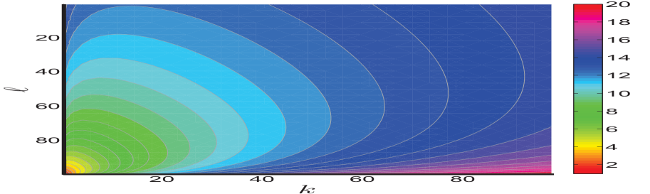
(a) The inter-layer joint degree distribution for preferential growth with $\beta_{1}=2$ and $\beta_{2}=4$, as given by Equation (6). The function decays fast in $k$ and $\ell$, so we have depicted the logarithm of the inverse of this function, for better visibility. Note the skew in the contours. Had $\beta_{1}$ and $\beta_{2}$ been equal, the distribution would be symmetric. The function attains its maximum at $k=\beta,1$ and $\ell=\beta_{2}$.

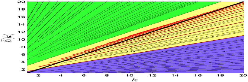
(b) $\overline{\ell}(k)$ for all combinations of $1\leq\beta_{1},\beta_{2}\leq 10$. There are three distinct regions. In the green region, $\overline{\ell}(k)>k$ regardless of $k,\beta_{1},\beta_{2}$. In the purple region, the converse is true. In the yellow region, $\overline{\ell}(k)>k$ up to some critical degree $k_{c}(\beta_{1},\beta_{2})$, and above the critical degree, $\overline{\ell}(k)<k$. The top boundary corresponds to the case of $\beta_{2}=2,\beta_{1}=1$ and the bottom one pertains to $\beta_{1}=\beta_{2}=1$.

Figure 1: Inter-layer joint degree distribution for preferential growth. The left figure also applies to the case of uniform growth. symmetric.

4 Model 2: Uniform Attachment in both Layers

In this model, we assume that each incoming node establishes links in both layers by selecting destinations from existing nodes uniformly at random. The rate equation (2) should be modified to the following:

$$\big{[}N(0)+t\big{]}\big{[}n_{k,\ell}(t+1)-n_{k,\ell}(t)\big{]}+n_{t+1}(k,\theta,\ell)=$$

$$+\beta_{1}\,\displaystyle\frac{N_{k-1,\ell}(t)-N_{k\ell}(t)}{N(0)+t}+\beta_{2}\,\displaystyle\frac{N_{t}(k,\theta,\ell-1)-N_{t}(k,\theta,\ell)}{N(0)+t}+\delta_{k\beta_{1}}\delta_{\ell\beta_{2}}.$$ (10)

Using the substitution $n_{k,\ell}(t)=\frac{N_{k\ell}(t)}{N(0)+t}$, this becomes

$$\big{[}N(0)+t\big{]}\big{[}n_{k,\ell}(t+1)-n_{k,\ell}(t)\big{]}+n_{t+1}(k,\theta,\ell)=$$

$$\beta_{1}\,\displaystyle\frac{N_{k-1,\ell}(t)-N_{k\ell}(t)}{N(0)+t}+\beta_{2}\,\displaystyle\frac{N_{t}(k,\theta,\ell-1)-N_{t}(k,\theta,\ell)}{N(0)+t}+\delta_{k\beta_{1}}\delta_{\ell\beta_{2}}.$$ (11)

In the steady state, that is, in the limit as ${t\rightarrow\infty}$, this becomes

$$n_{k\ell}=\beta_{1}\,\displaystyle\frac{n_{k-1,\ell}-n_{k,\ell}}{1}+\beta_{2}\,\displaystyle\frac{n_{k,\ell-1}-n_{k,\ell}}{1}+\delta_{k,\beta_{1}}\delta_{\ell,\beta_{2}}.$$ (12)

This can be simplified and equivalently expressed as follows

$$n_{k,\ell}=\,\displaystyle\frac{\beta_{1}}{1+\beta_{1}+\beta_{2}}n_{k-1,\ell}+\,\displaystyle\frac{\beta_{2}}{1+\beta_{1}+\beta_{2}}n_{k,\ell-1}+\,\displaystyle\frac{\delta_{k,\beta_{1}}\delta_{\ell,\beta_{2}}}{1+\beta_{1}+\beta_{2}}.$$ (13)

This difference equation is solved in Appendix 0.C. The solution is

$$n_{k,\ell}=\,\displaystyle\frac{\beta_{1}^{k-\beta_{1}}\beta_{2}^{\ell-\beta_{2}}\,\binom{k-\beta_{1}+\ell-\beta_{2}}{k-\beta_{1}}}{(1+\beta_{1}+\beta_{2})^{k-\beta_{1}+\ell-\beta_{2}+1}}$$ (14)

To find the conditional average degree, that is, $\bar{\ell}(k)$, we first need the degree distribution of single layers in order to constitute the conditional degree distribution. This is found previously for example in [13, 14]. The degree distribution in the first layer is $n_{k}=\frac{1}{\beta_{1}}\left(\frac{\beta_{1}}{\beta_{1}+1}\right)^{k-\beta_{1}+1}$. We need to compute

$$\bar{\ell}(k) =\,\displaystyle\sum_{\ell}\ell n_{\ell|k}=\,\displaystyle\sum_{\ell}\ell\,\displaystyle\frac{n_{k,\ell}}{n_{k}}=\,\displaystyle\sum_{\ell}\ell\,\displaystyle\frac{\,\displaystyle\frac{\beta_{1}^{k-\beta_{1}}\beta_{2}^{\ell-\beta_{2}}\,\binom{k-\beta_{1}+\ell-\beta_{2}}{k-\beta_{1}}}{(1+\beta_{1}+\beta_{2})^{k-\beta_{1}+\ell-\beta_{2}+1}}}{\frac{1}{\beta_{1}}\left(\frac{\beta_{1}}{\beta_{1}+1}\right)^{k-\beta_{1}+1}}$$

$$=\,\displaystyle\frac{(\beta_{1}+1)^{k-\beta_{1}+1}}{(\beta_{1}+\beta_{2}+1)^{k-\beta_{1}+1}}\,\displaystyle\sum_{\ell}\ell\frac{\beta_{2}^{\ell-\beta_{2}}\,\binom{k-\beta_{1}+\ell-\beta_{2}}{k-\beta_{1}}}{(1+\beta_{1}+\beta_{2})^{\ell-\beta_{2}}}$$ (15)

We have performed this summation in Appendix 0.D. The result is

$$\bar{\ell}(k)=\frac{\beta_{2}}{\beta_{1}+1}(k+2).$$ (16)

This is identical to (8).

5 Simulations

We performed Monte Carlo simulations to verify the results. Figure 2(a) depicts $\bar{\ell}(k)$ as a function of $k$ for both uniform and preferential attachment for $\beta_{1}=2,\beta_{2}=4$. The two curves are visibly linear and overlapping. Figure 2(b) depicts $\bar{\ell}(k)$ for both uniform and preferential attachment for $\beta_{1}=\beta_{2}=m$ for the cases $m=1,2,4,8$. It can be observed from Figure 2(b) that in all cases the curves for preferential and uniform growth overlap, and that the slope increases as $m$ increases. This is consistent with the predictions of (16) and (8), where the slope is given by $\frac{m}{m+1}$. This attains its minimum at $m=1$, and reaches unity for $m\rightarrow\infty$.

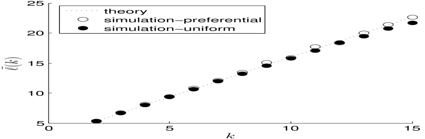
(a) $\beta_{1}=2,\beta_{2}=4$.

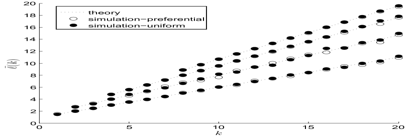
(b) $\beta_{1}=\beta_{2}=m$, for $m=1,2,4,8$.

Figure 2: $\overline{\ell}(k)$ for preferential and uniform growth. The left figure depicts $\overline{\ell}(k)$ for an example configuration of heterogeneous growth (i.e., $\beta_{1}\neq\beta_{2}$). The right figure represents results for homogeneous growth. It depicts different $\overline{\ell}(k)$ curves obtained for different values of $m$, where $\beta_{1}=\beta_{2}=m$ (the top line is for $m=8$, and the bottom-most line is for $m=1$). It can be seen that the slope of $\overline{\ell}(k)$ increases as $m$ increases. The results are averaged over 500 Monte Carlo Trials.

6 Summary and Future Work

We studied the problem of multiplex network growth, where two layers were heterogeneously growing. We considered the cases of preferential and uniform growth separately. We obtained the inter-layer joint degree distribution for both settings. We calculated $\overline{\ell}(k)$, and observed that it is identical in both scenarios. We corroborated the theoretical findings with Monte Carlo simulations.

While the average degree $\overline{\ell}(k)$ are calculated to be the same in Eqs. (8) and (16), it does not mean the two cases have entirely the same correlation properties. Note, for example, that it was obtained in [12] that the two cases have different inter-degree correlation coefficients.

Plausible extensions of the present analysis are as follows. First, there is no closed-form solution in the literature for the inter-layer joint degree distribution of growing multiplex networks with nonzero coupling, where the link reception probabilities in one layer depends on the degrees in both layers. Second, it would be informative to analyze the growth problem in arbitrary times, to grasp the finite size effects and to understand how $\overline{\ell}(k)$ evolves over time, and how the time evolution differs in the preferential and uniform settings. Third, it would plausible to endow the nodes with initial attractiveness, that is, to consider a shifted-linear kernel for the preferential growth mechanism. Fourth, a more realistic and practical model would require intrinsic fitness values for nodes, so it would be plausible to analyze the multiplex growth problem with intrinsic fitness. Finally, since most real systems are multi-layer, it would be plausible to extend the bi-layer results to arbitrary $M>2$ layers.

Appendix 0.A Solving Difference Equation (5)

We need to solve

$$n_{k\ell}=\,\displaystyle\frac{k-1}{k+\ell+2}n_{k-1,\ell}\,\displaystyle\frac{\ell-1}{k+\ell+2}n_{k,\ell-1}+\,\displaystyle\frac{2\delta_{k\beta_{1}}\delta_{\ell\beta_{2}}}{2+\beta_{1}+\beta_{2}}.$$ (17)

We define the new sequence

$$m_{k\ell}\,\stackrel{{\scriptstyle\text{def}}}{{=}}\,\displaystyle\frac{(k+\ell+2)!}{(k-1)!(\ell-1)!}n_{k\ell}.$$ (18)

The following holds

$$\begin{cases}\,\displaystyle\frac{k-1}{k+\ell+2}n_{k-1,\ell}=\,\displaystyle\frac{(k-1)!(\ell-1)!}{n}_{k\ell}{(k+\ell+2)!}m_{k-1,\ell}\\ \\ \,\displaystyle\frac{\ell-1}{k+\ell+2}n_{k,\ell-1}=\,\displaystyle\frac{(k-1)!(\ell-1)!}{n}_{k\ell}{(k+\ell+2)!}m_{k,\ell-1}.\end{cases}$$ (19)

Plugging these into (17), we can recast it as

$$m_{k\ell}=m_{k-1,\ell}+m_{k,\ell-1}+2\,\displaystyle\frac{(\beta_{1}+\beta_{2}+1)!}{(\beta_{1}-1)!(\beta_{2}-1)!}\delta_{k\beta_{1}}\delta_{\ell\beta_{2}}.$$ (20)

Now define the Z-transform of sequence $m_{k,\ell}$ as follows:

$$\begin{cases}\psi(z,y)\,\stackrel{{\scriptstyle\text{def}}}{{=}}\,\displaystyle\sum_{k}\sum_{\ell}m_{k,\ell}z^{-k}y^{-\ell}\\ m_{k,\ell}=\,\displaystyle\frac{1}{(2\pi i)^{2}}\,\displaystyle\oint\oint\psi(z,y)z^{k-1}y^{\ell-1}dzdy.\end{cases}$$ (21)

Taking the Z transform of every term in (20), we arrive at

$$\psi(z,y)= z^{-1}\psi(z,y)+y^{-1}\psi(z,y)+2\,\displaystyle\frac{(\beta_{1}+\beta_{2}+1)!}{(\beta_{1}-1)!(\beta_{2}-1)!}z^{-\beta_{1}}y^{-\beta_{2}}.$$ (22)

This can be rearranged and rewritten as follows

$$\psi(z,y)=\,\displaystyle\frac{2}{1-z^{-1}-y^{-1}}\,\displaystyle\frac{(\beta_{1}+\beta_{2}+1)!}{(\beta_{1}-1)!(\beta_{2}-1)!}z^{-\beta_{1}}y^{-\beta_{2}}$$ (23)

The inverse transform is given by

$$m_{k,\ell}=\,\displaystyle\frac{2(\beta_{1}+\beta_{2}+1)!}{(\beta_{1}-1)!(\beta_{2}-1)!}\oint\oint\,\displaystyle\frac{z^{k-\beta_{1}-1}y^{\ell-\beta_{2}-1}dzdy}{(-4\pi^{2})(1-z^{-1}-y^{-1})}$$

$$=\,\displaystyle\frac{2(\beta_{1}+\beta_{2}+1)!}{(\beta_{1}-1)!(\beta_{2}-1)!}\oint\oint\,\displaystyle\frac{z^{k-\beta_{1}}y^{\ell-\beta_{2}}dzdy}{(-4\pi^{2})(zy-z-y)}$$

$$=\,\displaystyle\frac{2(\beta_{1}+\beta_{2}+1)!}{(\beta_{1}-1)!(\beta_{2}-1)!}\oint\oint\,\displaystyle\frac{z^{k-\beta_{1}}y^{\ell-\beta_{2}}dzdy}{(-4\pi^{2})(y-1)\big{[}z-\frac{y}{y-1}\big{]}}.$$ (24)

First we integrate over $z$. We get

$$m_{k,\ell} =\,\displaystyle\frac{2(\beta_{1}+\beta_{2}+1)!}{(\beta_{1}-1)!(\beta_{2}-1)!}\oint\,\displaystyle\frac{\left(\frac{y}{y-1}\right)^{k-\beta_{1}}y^{\ell-\beta_{2}}dy}{(2\pi i)(y-1)}$$

$$=\,\displaystyle\frac{2(\beta_{1}+\beta_{2}+1)!}{(\beta_{1}-1)!(\beta_{2}-1)!}\oint\,\displaystyle\frac{y^{k-\beta_{1}+\ell-\beta_{2}}dy}{(2\pi i)(y-1)^{k-\beta_{1}+1}}.$$ (25)

Now note that the residue of $\,\displaystyle\frac{f(y)}{(y-1)^{n}}$ for positive integer equals $\,\displaystyle\frac{f^{(n-1)}(1)}{(n-1)!}$, where the numerator denotes the ${(n-1)}$th derivative of the function $f(y)$, evaluated at ${y=1}$. Also, note that the $m$-th derivative of the function $y^{n}$, for integer $n$ and $m$, equals $\,\displaystyle\frac{m!}{(n-m)!}y^{n-m}$. Combining these two facts, we obtain

$$m_{k,\ell}=\,\displaystyle\frac{2(\beta_{1}+\beta_{2}+1)!}{(\beta_{1}-1)!(\beta_{2}-1)!}\,\binom{k-\beta_{1}+\ell-\beta_{2}}{k-\beta_{1}}.$$ (26)

Using (18), we arrive at

$$n_{k,\ell}=\,\displaystyle\frac{2(\beta_{1}+\beta_{2}+1)!}{(\beta_{1}-1)!(\beta_{2}-1)!}\,\displaystyle\frac{1}{k(k+1)\ell(\ell+1)}\,\displaystyle\frac{\,\binom{k-\beta_{1}+\ell-\beta_{2}}{k-\beta_{1}}}{\,\binom{k+\ell+2}{k+1}}.$$ (27)

This can be equivalently expressed as follows:

$$n_{k,\ell}=\,\displaystyle\frac{2\beta_{1}(\beta_{1}+1)\beta_{2}(\beta_{2}+1)}{(\beta_{1}+\beta_{2}+2)k(k+1)\ell(\ell+1)}\,\displaystyle\frac{\,\binom{\beta_{1}+\beta_{2}+2}{\beta+1}}{\,\binom{k+\ell+2}{k+1}}\,\binom{k-\beta_{1}+\ell-\beta_{2}}{k-\beta_{1}}.$$ (28)

Appendix 0.B Performing the Summation in (7)

We need to calculate

$$\bar{\ell}(k)=\,\displaystyle\sum_{\ell}\frac{\beta_{2}(\beta_{2}+1)}{(2+\beta_{1}+\beta_{2})}\frac{\,\binom{\beta_{1}+\beta_{2}+2}{\beta+1}\,\binom{k-\beta_{1}+\ell-\beta_{2}}{k-\beta_{1}}}{\,\binom{k+\ell+2}{\ell}}.$$ (29)

We use the following identity: $\frac{1}{\,\binom{n}{m}}=(n+1)\int_{0}^{1}t^{n}(1-t)^{n-m}dt,$ to rewrite the binomial reciprocal of the coefficient as follows

$$\,\displaystyle\frac{1}{\,\binom{k+\ell+2}{\ell}}=(k+\ell+3)\,\displaystyle\int_{0}^{1}t^{\ell}(1-t)^{k+2}dt.$$ (30)

Also, from Taylor expansion, it is elementary to show that

$$S_{1}(x,n)\,\stackrel{{\scriptstyle\text{def}}}{{=}}\,\displaystyle\sum_{m}x^{m}\,\binom{m}{n}=\,\displaystyle\frac{x^{n}}{(1-x)^{n+1}}.$$ (31)

This identity will be used in the steps below. Plugging (30) into (33), we have

$$\bar{\ell}(k) =\,\displaystyle\sum_{\ell}\frac{\beta_{2}(\beta_{2}+1)}{(2+\beta_{1}+\beta_{2})}\frac{\,\binom{\beta_{1}+\beta_{2}+2}{\beta+1}\,\binom{k-\beta_{1}+\ell-\beta_{2}}{k-\beta_{1}}}{\,\binom{k+\ell+2}{\ell}}$$

$$\leavevmode\resizebox{411.93767pt}{}{$=\,\displaystyle\frac{\beta_{2}(\beta_{2}+1)}{(2+\beta_{1}+\beta_{2})}\,\binom{\beta_{1}+\beta_{2}+2}{\beta_{1}+1}\,\displaystyle\int_{0}^{1}(1-t)^{k+2}t^{-k-2}\,\displaystyle\frac{d}{dt}\left[t^{3+\beta_{1}+\beta_{2}}\,\displaystyle\sum_{\ell}t^{k-\beta_{1}+\ell-\beta_{2}}\,\binom{k-\beta_{1}+\ell-\beta_{2}}{k-\beta_{1}}\right]dt$}.$$ (32)

Using (31), this becomes:

$$\overline{\ell}(k) =\,\displaystyle\frac{\beta_{2}(\beta_{2}+1)}{(2+\beta_{1}+\beta_{2})}\,\binom{\beta_{1}+\beta_{2}+2}{\beta_{1}+1}\,\displaystyle\int_{0}^{1}(1-t)^{k+2}t^{-k-2}\,\displaystyle\frac{d}{dt}\left[t^{3+\beta_{1}+\beta_{2}}\,\displaystyle\frac{t^{k-\beta_{1}}}{(1-t)^{k-\beta_{1}+1}}\right]dt$$

$$=\,\displaystyle\frac{\beta_{2}(\beta_{2}+1)}{(2+\beta_{1}+\beta_{2})}\,\binom{\beta_{1}+\beta_{2}+2}{\beta_{1}+1}\,\displaystyle\int_{0}^{1}(1-t)^{k+2}t^{-k-2}\,\displaystyle\frac{d}{dt}\left[\,\displaystyle\frac{t^{k+\beta_{2}+3}}{(1-t)^{k-\beta_{1}+1}}\right]dt$$

$$=\frac{\beta_{2}(\beta_{2}+1)\beta_{1}!\beta_{2}!}{(2+\beta_{1}+\beta_{2})(1+\beta_{1}+\beta_{2})!}\,\binom{\beta_{1}+\beta_{2}+2}{\beta_{1}+1}\left[(k+\beta_{2}+3)-(\beta_{2}+1)\right]$$

$$=\,\displaystyle\frac{\beta_{2}}{\beta_{1}+1}(k+2)$$ (33)

Appendix 0.C Solving Difference Equation (13)

Let us repeat the equation we need to solve for easy reference

$$n_{k,\ell}=\,\displaystyle\frac{\beta_{1}}{1+\beta_{1}+\beta_{2}}n_{k-1,\ell}+\,\displaystyle\frac{\beta_{2}}{1+\beta_{1}+\beta_{2}}n_{k,\ell-1}+\,\displaystyle\frac{\delta_{k,\beta_{1}}\delta_{\ell,\beta_{2}}}{1+\beta_{1}+\beta_{2}}.$$ (34)

Let us define the following quantities from brevity:

$$q_{1}\,\stackrel{{\scriptstyle\text{def}}}{{=}}\,\displaystyle\frac{\beta_{1}}{1+\beta_{1}+\beta_{2}}~{}~{}~{}~{},~{}~{}~{}~{}q_{2}\,\stackrel{{\scriptstyle\text{def}}}{{=}}\,\displaystyle\frac{\beta_{2}}{1+\beta_{1}+\beta_{2}}$$ (35)

Taking the Z transform from both sides of (34), we get

$$\psi(z,y)=q_{1}z^{-1}\psi(z,y)+q_{2}y^{-1}\psi(z,y)+\,\displaystyle\frac{z^{-\beta_{1}}y^{-\beta_{2}}}{1+\beta_{1}+\beta_{2}}.$$ (36)

This can be rearranged and recast as

$$\psi(z,y)=\,\displaystyle\frac{1}{1-q_{1}z^{-1}-q_{2}y^{-1}}\,\displaystyle\frac{z^{-\beta_{1}}y^{-\beta_{2}}}{1+\beta_{1}+\beta_{2}}.$$ (37)

This can be inverted through the following steps

$$n_{k\ell} =\,\displaystyle\frac{1}{(1+\beta_{1}+\beta_{2})(2\pi i)^{2}}\,\displaystyle\oint\psi(z,y)z^{k-1}y^{\ell-1}dzdy$$

$$=\,\displaystyle\frac{1}{(1+\beta_{1}+\beta_{2})(2\pi i)^{2}}\,\displaystyle\oint\oint\,\displaystyle\frac{z^{k-\beta-1}y^{\ell-\beta-1}}{1-q_{1}z^{-1}-q_{2}y^{-1}}dzdy$$

$$=\,\displaystyle\frac{1}{(1+\beta_{1}+\beta_{2})(2\pi i)^{2}}\,\displaystyle\oint\oint\,\displaystyle\frac{z^{k-\beta_{1}}y^{\ell-\beta_{2}}}{zy-yq_{1}-zq_{2}}dzdy$$

$$=\,\displaystyle\frac{1}{(1+\beta_{1}+\beta_{2})(2\pi i)^{2}}\,\displaystyle\oint\oint\,\displaystyle\frac{z^{k-\beta_{1}}y^{\ell-\beta_{2}}}{z-\frac{yq_{1}}{y-q_{2}}}\,\displaystyle\frac{1}{y-q_{2}}dzdy.$$ (38)

There is a single simple pole at $z=\frac{yq_{1}}{y-q_{2}}$, which renders the integral trivial:

$$n_{k\ell} =\,\displaystyle\frac{\oint\frac{y^{\ell-\beta_{2}}}{y-q_{2}}\left(\frac{yq_{1}}{y-q_{2}}\right)^{k-\beta_{1}}dzdy}{(1+\beta_{1}+\beta_{2})(2\pi i)}=\,\displaystyle\frac{q_{1}^{k-\beta_{1}}\,\displaystyle\oint\,\displaystyle\frac{y^{k-\beta_{1}+\ell-\beta_{2}}}{(y-q_{2})^{k-\beta_{1}+1}}dzdy}{(1+\beta_{1}+\beta_{2})(2\pi i)}$$

(39)

After inserting the expressions for $q_{1},q_{2}$ from (35), this becomes

$$n_{k,\ell}=\,\displaystyle\frac{\beta^{k-\beta_{1}}\beta_{2}^{\ell-\beta_{2}}\,\binom{k-\beta_{1}+\ell-\beta_{2}}{k-\beta_{1}}}{(1+\beta_{1}+\beta_{2})^{k-\beta_{1}+\ell-\beta_{2}+1}}.$$ (40)

Appendix 0.D Performing the Summation in (15)

We need to perform the following summation:

$$\bar{\ell}(k) =\,\displaystyle\frac{(\beta_{1}+1)^{k-\beta_{1}+1}}{(\beta_{1}+\beta_{2}+1)^{k-\beta_{1}+1}}\,\displaystyle\sum_{\ell}\ell\frac{\beta_{2}^{\ell-\beta_{2}}\,\binom{k-\beta_{1}+\ell-\beta_{2}}{k-\beta_{1}}}{(1+\beta_{1}+\beta_{2})^{\ell-\beta_{2}}}$$ (41)

Let us denote $k-\beta_{1}$ by $k^{\prime}$ and $\ell-\beta_{2}$ by $\ell^{\prime}$. Also let us denote $\frac{\beta_{2}}{1+\beta_{1}+\beta_{2}}$ by $x$. We need to evaluate the following sum: ${\sum_{\ell^{\prime}}(\ell^{\prime}+\beta_{2})x^{\ell^{\prime}}\,\binom{k^{\prime}+\ell^{\prime}}{k^{\prime}}}$. Let us use (31) and define $S_{1}(x,n)\,\stackrel{{\scriptstyle\text{def}}}{{=}}\sum_{m}x^{m}\,\binom{m}{n}=\frac{x^{n}}{(1-x)^{n+1}}$. We have:

$$\sum_{\ell^{\prime}}(\beta_{2}+\ell^{\prime})x^{\ell^{\prime}}\,\binom{k^{\prime}+\ell^{\prime}}{k^{\prime}}=\beta_{2}x^{-k^{\prime}}S_{1}(x,k^{\prime})+x\sum_{\ell^{\prime}}\ell^{\prime}x^{\ell^{\prime}-1}\,\binom{k^{\prime}+\ell^{\prime}}{k^{\prime}}$$

$$=\,\displaystyle\frac{1}{(1-x)^{k^{\prime}+2}}\big{[}\beta_{2}+x(k^{\prime}+1-\beta_{2})\big{]}.$$ (42)

Replacing $x$ with $\frac{\beta_{2}}{1+\beta_{1}+\beta_{2}}$ and inserting this result into (41), we get

$$\,\displaystyle\frac{1}{[1-(\frac{\beta_{2}}{1+\beta_{1}+\beta_{2}})]^{k-\beta_{1}+2}}\big{[}\beta_{2}+\frac{\beta_{2}}{1+\beta_{1}+\beta_{2}}(k-\beta_{1}+1-\beta_{2})\big{]}$$

$$=\,\displaystyle\frac{(1+\beta_{1}+\beta_{2})^{k-\beta_{1}+2}}{(1+\beta_{1})^{k-\beta_{1}+2}}\big{[}\beta_{2}+2+\frac{\beta_{2}}{1+\beta_{1}+\beta_{2}}(k-\beta_{1}+1-\beta_{2})\big{]}$$

$$=\,\displaystyle\frac{(1+\beta_{1}+\beta_{2})^{k-\beta_{1}+2}}{(1+\beta_{1})^{k-\beta_{1}+2}}\big{[}\frac{\beta_{2}(k+2)}{1+\beta_{1}+\beta_{2}}\big{]}$$ (43)

Plugging this into (41), we get

$$\bar{\ell}(k) =\frac{\beta_{2}(k+2)}{1+\beta_{1}}$$ (44)

References

• [1] De Domenico, M., Sole-Ribalta, A., Cozzo, E., Kivela, M., Moreno, Y., Porter, M. A., Gomez, S., Arenas, A.: Mathematical formulation of multilayer networks, Phys. Rev. X 3, 041022 (2013).
• [2] Kivela, A., Arenas, A., Barthelemy, M., Gleeson, J., Moreno, Y., Porter, M.: Multilayer Networks, J. Complex Netw. 2, 203-271 (2014).
• [3] Son, S. W., Bizhani, G., Christensen, C., Grassberger, P., Paczuski, M.: Percolation theory on interdependent networks based on epidemic spreading, Europhysics Lett. 97, 16006 (2012).
• [4] Granell, C., Gomez, S., Arenas, A.: Dynamical interplay between awareness and epidemic spreading in multiplex networks, Phy. Rev. Lett. 111, 128701 (2013).
• [5] Cellai, D., Lopez, E., Zhou, J., Gleeson, J. P., Bianconi, G.: Percolation in multiplex networks with overlap, Phys. Rev. E, 88, 052811 (2013).
• [6] Gomez-Gardenes, J., Reinares, I., Arenas, A., Floria, L. M. : Evolution of cooperation in multiplex networks, Sci. Rep. 2, 620 (2012).
• [7] Gomez, S., Diaz-Guilera, A., Gomez-Gardenes, J., Perez-Vicente, C. J., Moreno, Y., Arenas, A.: Diffusion dynamics on multiplex networks. Phys. Rev. Lett. 110, 028701 (2013).
• [8] Cozzo, E., Banos, R. A., Meloni, S., Moreno, Y. : Contact-based social contagion in multiplex networks. Phys. Rev. E 8, 050801 (2013).
• [9] Boccaletti, S., Bianconi, G., Criado, R., Del Genio, C. I., Gómez-Gardenes, J., Romance, M., Sendina-Nadal, I, Zanin, M. : The structure and dynamics of multilayer networks, Phys. Rep. 544, 1–122. (2014).
• [10] Barabasi, A. L., Albert, R. : Emergence of scaling in random networks, Science, 286, 509–512 (1999).
• [11] Nicosia, V., Bianconi, G., Latora, V., Barthelemy, V.: Non-linear growth and condensation in multiplex networks, Phys. Rev. E 90, 042807 (2014)
• [12] Kim, Jung Yeol, and K-I. Goh. : Coevolution and correlated multiplexity in multiplex networks., Phys. Rev. Lett. 111.5 (2013): 058702.
• [13] Nicosia, V., Bianconi, G., Latora, V., Barthelemy, M.: Growing multiplex networks, Phys. Rev. Lett. 111, 058701 (2013).
• [14] Fotouhi, B., Rabbat, M., Network growth with arbitrary initial conditions: Degree dynamics for uniform and preferential attachment, Phys. Rev. E 88, 062801 (2013).