An explicit high-order single-stage single-step positivity-preserving finite difference WENO method for the compressible Euler equations

Abstract

In this work we construct a high-order, single-stage, single-step positivity-preserving method for the compressible Euler equations. Space is discretized with the finite difference weighted essentially non-oscillatory (WENO) method. Time is discretized through a Lax-Wendroff procedure that is constructed from the Picard integral formulation (PIF) of the partial differential equation. The method can be viewed as a modified flux approach, where a linear combination of a low- and high-order flux defines the numerical flux used for a single-step update. The coefficients of the linear combination are constructed by solving a simple optimization problem at each time step. The high-order flux itself is constructed through the use of Taylor series and the Cauchy-Kowalewski procedure that incorporates higher-order terms. Numerical results in one- and two-dimensions are presented.

1 Introduction

The objective of this work is to define a single-stage, single-step finite difference WENO method that is provably positivity-preserving for the compressible Euler equations. These equations describe the evolution of density $\rho$, momentum $\rho\vec{u}$ and energy $\mathcal{E}$ of an ideal gas through

$$\left(\begin{array}[]{c}\rho\\ \rho\vec{u}\\ \mathcal{E}\end{array}\right)_{,t}+\nabla_{\bf x}\cdot\left(\begin{array}[]{c}\rho\vec{u}\\ \rho\vec{u}\otimes\vec{u}+p{\bf I}\\ (\mathcal{E}+p)\vec{u}\end{array}\right)=0.$$ (1)

The energy $\mathcal{E}$ is related to the primitive variables $\rho$, $\vec{u}$ and pressure $p$ by the equation of state that we take to be $\mathcal{E}=\frac{p}{\gamma-1}+\frac{1}{2}\rho\lVert\vec{u}\rVert^{2}$. The ratio of specific heats is the constant $\gamma$. Numerical difficulties for solving this system include the following:

• Low (1st and 2nd) order methods generally suffer from an inordinate amount of numerical diffusion. However, they are oftentimes more robust, and in some cases they have provable convergence to the correct entropy solution. Historically, 2nd-order schemes LxW60 ; Sod78 ; Harten78 ; Roe81 have been called “high-resolution” methods when compared to their 1st-order counterparts VonRict50 ; CoIsRe52 ; Lax54 ; God57 .

• High-order methods HaEnOsCh87 ; ShuOsher87 ; LiuOsherChan94 provide greater accuracy and resolution for much less overall computational effort. However, they are oftentimes less robust, and do not necessarily have provable convergence to the correct entropy solution.

In this work, we define a high-order conservative finite difference method based upon the Picard integral formulation of the PDE. We make a further modification to the fluxes and define a numerical scheme that obtains the following properties:

• High-order accuracy in space ($5^{th}$-order) and time ($3^{rd}$-order). Our method can be extended to arbitrary order in space or time.

• A robust scheme that stems from provable positivity preservation of the pressure and density. Numerical results indicate that high-order accuracy is retained with our positivity-preserving limiter turned on.

Our scheme is the first single-stage, single-step numerical method that simultaneously attains high-order accuracy, with provable positivity preservation. When compared to other positivity-preserving schemes, our method has the following advantages:

• In order to retain positivity, we only solve one simple optimization problem per time step. Unlike positivity-“preserving” methods that use Runge-Kutta discretizations XiQiXu14 ; ChLiTaXu14 , positivity of our solution is guaranteed during the entire simulation because we do not have internal stages where the solution can go negative.

• Compared to other positivity-preserving schemes ZhangShu11-survey ; ZhangShu12 , the addition of the positivity preserving limiter introduces none of the additional time step restrictions that are often introduced in order to retain positivity.

In addition, our method is amenable to adaptive mesh refinement (AMR) technology. At present, we aim to lay the necessary foundation that would be required to do so. An in depth investigation of this property is the subject of a future study.

1.1 An overview of the proposed method

The Euler equations define a system of hyperbolic conservation laws. In 1D, such an equation is given by

$$q_{,t}+f(q)_{\!,\,x}=0,$$ (2)

where $q(t,x):\mathbb{R}^{+}\times\mathbb{R}\to\mathbb{R}^{m}$ is the unknown vector of $m$ conserved quantities and $f:\mathbb{R}^{m}\to\mathbb{R}^{m}$ is a prescribed flux function. The conserved variables for the 1D Euler equations are $q=\left(\rho,\rho u^{1},\mathcal{E}\right)^{T}$. A typical finite difference solver for (2) discretizes space with a uniform grid of $m_{x}$ equidistant points in $\Omega=[a,b]$,

$$x_{i}=a+\left(i-\frac{1}{2}\right)\Delta x,\qquad\Delta x=\frac{b-a}{m_{x}},\qquad i\in\{1,\dots,m_{x}\},$$ (3)

and looks for a pointwise approximation $q_{i}^{n}\approx q(t^{n},x_{i})$ solution to hold at discrete time levels $t^{n}$. In a conservative finite difference WENO method, the update of the unknowns is typically defined by

$$q^{n+1}_{i}=q^{n}_{i}-\frac{\Delta t}{\Delta x}\left({F}^{n}_{i+\frac{1}{2}}-{F}^{n}_{i-\frac{1}{2}}\right),$$ (4)

where the numerical flux ${F}^{n}_{i\pm\frac{1}{2}}$ is constructed from a linear combination of the WENO reconstruction procedure applied to stage values from a Runge-Kutta solver.

In this work, we propose the following procedure:

1. Construct a high-order approximation to the time-averaged fluxes HaEnOsCh87 ; SeGuCh14

   $${F}^{n}_{i}:=\frac{1}{\Delta t}\int_{t^{n}}^{t^{n+1}}f(q(t,x_{i}))\,dt$$ (5)

   at each grid point $x_{i}$. In this work, we consider the Taylor discretization of Eqn. (5) for conservative finite difference methods.

2. Construct a high-order in space and time numerical flux $\hat{F}^{n}_{i-\frac{1}{2}}$ based upon applying the WENO reconstruction procedure to the time-averaged fluxes SeGuCh14 .

3. Replace the flux constructed in Step 2 with

   $$\tilde{F}^{n}_{i-\frac{1}{2}}:=\theta^{n}_{i-\frac{1}{2}}(\hat{F}^{n}_{i-\frac{1}{2}}-\hat{f}^{n}_{i-\frac{1}{2}})+\hat{f}^{n}_{i-\frac{1}{2}},$$ (6)

   where $\theta^{n}_{i-\frac{1}{2}}\in[0,1]$ is found by solving a single optimization problem, and $\hat{f}^{n}_{i-\frac{1}{2}}$ is a low-order flux that guarantees positivity of the solution. This procedure is described in §4.

4. Insert the result of Step 3 into Eqn. (4), and update the solution.

Steps 1 and 2 have already been proposed in SeGuCh14 , where high-order accuracy is obtained through a flux modification that incorporates the high-order temporal discretization. A review of this procedure is presented in §3. Step 3 can be thought of as a further flux modification, where an automatic switch adjusts between the high-order non positivity-preserving scheme, and a low-order, positivity-preserving scheme. The original idea is attributed to Harten and Zwas HaZw72 , but has since been extended to high-order WENO schemes XiQiXu14 . The details of this procedure are presented in §4 and §5.

2 Background

The compressible Euler equations have been an object of study ever since the infancy of numerical methods VonRict50 ; CoIsRe52 ; Lax54 ; God57 ; LxW60 . In recent years, high-order methods have attracted considerable interest because of their ability to obtain higher accuracy on certain problems with an equivalent computational cost of a low-order method. Among many choices of high-order schemes are the classical essentially non-oscillatory (ENO) method HaEnOsCh87 , the extensions to finite difference (FD) and finite volume (FV) WENO methods LiuOsherChan94 ; JiangShu96 ; Shu09 , and the discontinuous Galerkin (DG) method colish89 . These methods all seek to simultaneously obtain two properties: retain high-order accuracy in smooth regions, and capture shocks without introducing spurious oscillations near discontinuities of the solution. One added difficulty with high-order schemes is the necessity of defining and selecting a high-order time integrator. Runge-Kutta methods applied to the method of lines (MOL) approach is the most widely used discretization for high-order schemes. These methods all treat space and time as separate entities.

Over the past decade, there has been a rejuvenation of interest in high-order single-stage, single-step methods for hyperbolic conservation laws, including the compressible Euler equations. All of these methods are typically based upon a Taylor temporal discretization that uses the Cauchy-Kowalewski procedure to exchange temporal for spatial derivatives. Lax and Wendroff performed this very procedure in 1960 LxW60 , and this technique has since been called the Lax-Wendroff procedure within the numerical analysis community. Methods for defining a second and higher-order single-step version of Godunov’s method were investigated in the 1980s Ro87 ; BeCoTr89 ; Me90 . The original high-order ENO method of Harten et. al HaEnOsCh87 used Taylor series for their temporal discretization, although most of the attention they have received is for their emphasis on the spatial discretization. In 2001, the preliminary definitions for the so-called Arbitrary DERivative (ADER) methods toro2001 ; ToroTitarev02 ; TitarevToro02-ader were put in place. Additionally, various FD WENO methods with Lax-Wendroff time discretizations have been constructed and tested on the Euler equations QiuShu03 ; JiangShuZhang13 ; SeGuCh14 . Recent ADER methods have been defined by Balsara and collaborators for hydrodynamics and magnetohydrodynamics balsara09 ; BaDiMeDuHuXu13 , and have later been extended to an adaptive mesh refinement (AMR) setting balsara13 . Other recent work in single-stage, single-step methods for Euler equations includes Lax-Wendroff time stepping coupled with DG QiuDumbserShu05 ; DuMu06 ; GaDuHiMuCl11 , and high-order Lagrangian schemes LiuChengShu09 . The present work is an extension of the Taylor discretization of the Picard integral formulation that uses finite differences for its spatial discretization SeGuCh14 , which falls into this single-stage, single-step class of methods.

Defining high-order numerical schemes that retain positivity of the solution for hydrodynamics (or magnetohydrodynamics) simulations is genuinely a non-trivial task. This has been an ongoing subject of study even for low and the so-called “high-resolution” schemes EinfMuRoeSj91 ; EstVil95 ; EsVi96 ; PeShu96 ; TangXu99 ; Dubroca99 ; TangXu00 ; Gallice03 . All methods that are second or higher order share the same disadvantage that without care, they may violate a natural weak stability condition that the density and pressure need to keep positive, which is necessary to ensure physical meaningfulness of the solution and hyperbolicity of the mathematical problem. Of some of the early positivity works, Perthame and Shu propose a general reconstruction approach to obtain a high-order positivity-preserving finite volume schemes from a low-order scheme PeShu96 . In addition, they prove that the explicit Lax-Friedrichs scheme is positivity-preserving with a CFL number up to $0.5$. Later on, a more general result extends the positivity-preserving property to CFL numbers up to $1$ for both explicit and implicit Lax-Friedrichs methods TangXu00 . With those building blocks, a positivity-preserving limiter is proposed for DG schemes ZhangShu10 ; ZhangShu11-euler ; ZhangXiaShu12 ; KoEk13 and FD and FV WENO schemes ZhangShu11-survey ; ZhangShu12 for the Euler equations. In hu2013 , a flux cut-off limiter is also applied to FD WENO schemes to retain positivity. In addition to gas dynamics, plasma physics is another area where retaining positivity of numerical solutions is critical, and therefore has seen recent attention in the literature RoSe11 ; GuChHi14 . For example, collision operators for Vlasov equations require a positive distribution function in order to avoid creating artificial singularities.

Our method is based upon a parameterized flux limiter that can be dated back to at least 1972 with the work of Harten and Zwas HaZw72 . There, the authors propose a second-order shock-capturing self adjusting hybrid scheme through a simple linear combination of low- and high-order fluxes that is identical to Eqn. (6). The original idea is to combine a “high-order” flux with a first-order flux such that it has better accuracy in smooth region and produces a smooth profile around shock regions. A similar approach called flux-corrected transport is proposed by Boris and Book Boris197338 ; Book1975248 ; Boris1976397 ; BoBoZa81 , where the purpose of limiting the high-order flux is to control overshoots and undershoots around shock regions. Sod performs an extensive review of these and other classical finite difference methods in a classical paper Sod78 . Xu and Lian recently extend this work to WENO methods that maintain the maximum-principle-preserving property for scalar hyperbolic conservation laws with the so-called “parametrized flux limiter” xu2013 ; liang2014parametrized . Later on, these limiters are applied to FD WENO schemes on rectangular meshes XiQiXu13 and FV WENO schemes on triangular meshes ChLiTaXu14 for the Euler equations. These limiters are also applied to magnetohydrodynamics with a constrained transport framework tang14 . The basic idea for all of these methods is the same: modify the high-order non positivity-preserving numerical flux by a linear combination of a low- and high-order flux in order to retain positivity of the solution. The modification is carefully designed so that the high-order accuracy remains.

The purpose of this work is to define a single-stage, single-step finite difference WENO method that is provably positivity-preserving for the compressible Euler equations. Of the various finite difference schemes constructed from the Picard integral formulation SeGuCh14 , we begin with the Taylor discretization, and then apply recently developed flux limiters XiQiXu13 ; ChLiTaXu14 in order to retain positivity of the solution. One advantage of the chosen limiter is that positivity is preserved without introducing additional time step restrictions, however, our primary contribution is that the present method is the first scheme to simultaneously be high-order, single-stage, single-step and have provable positivity preservation.

The outline of this paper is as follows. In §3, we briefly review the high-order finite difference WENO method that is based upon the Picard integral formulation of the PDE with a Taylor temporal discretization SeGuCh14 . In §4 and §5, we present the positivity-preserving limiter for PIF-WENO schemes applied to the compressible Euler system in single and multiple dimensions. Numerical examples of the positivity-preserving PIF-WENO scheme applied to the problems with low density and low pressure is provided in §6. Finally, conclusions and future work are given in §7.

3 A single-stage single-step finite difference WENO method

The numerical method that is the subject of this work is based upon the Taylor discretization of the Picard integral formulation of Euler’s equations, which is one of the many methods developed in SeGuCh14 . Our focus is on the finite difference WENO method based on a Taylor discretization of the time-averaged fluxes because it easily lends itself to the positivity-preserving limiters that are presented in §4. In this section, we review the minimal details presented in SeGuCh14 that are necessary to reproduce the present work. In addition, this section serves to set the notation that is used in upcoming sections.

In two dimensions, a hyperbolic conservation law is defined by a flux function with two components,

$$q_{t}+f(q)_{,x}+g(q)_{,y}=0,$$ (7)

where $q(t,x,y):\mathbb{R}^{+}\times\mathbb{R}^{2}\to\mathbb{R}^{m}$ is the vector of conserved variables, and $f,g:\mathbb{R}^{m}\to\mathbb{R}^{m}$ are the two components of the flux function. The Euler equations are an example of a set of equations from this class of problems.

Formal integration of (7) in time over $t\in[t^{n},t^{n+1}]$ defines the 2D Picard integral formulation SeGuCh14 as

$$q^{n+1}=q^{n}-\Delta t\left(F^{n}(x,y)\right)_{,x}-\Delta t\left(G^{n}(x,y)\right)_{,y},$$ (8a)

where the time-averaged flux is defined as

$${F}^{n}(x,y):=\frac{1}{\Delta t}\int_{t^{n}}^{t^{n+1}}f(q(t,x,y))\,dt,\quad{G}^{n}(x,y):=\frac{1}{\Delta t}\int_{t^{n}}^{t^{n+1}}g(q(t,x,y))\,dt.$$ (8b)

The basic idea of the Picard integral formulation of WENO (PIF-WENO) SeGuCh14 is to first approximate the time-averaged fluxes (5) at each grid point using some temporal discretization, and then approximate spatial derivatives in (8a) by applying WENO reconstruction to the resulting time-averaged fluxes. In this work, we approximate Eqn. (8a) with the finite difference WENO method, and we use a third-order Taylor discretization for (8b). We remark that the positivity-preserving limiter proposed in §4 can be generally applied to any form of the Picard integral formulation, including Runge-Kutta time discretizations.

Given a domain $\Omega=[a_{x},b_{x}]\times[a_{y},b_{y}]$, a finite difference approximation seeks pointwise approximations $q^{n}_{i,j}\approx q\left(t^{n},x_{i},y_{j}\right)$ to hold at each

$$x_{i} =a_{x}+\left(i-\frac{1}{2}\right)\Delta x,\qquad \Delta x=\frac{b_{x}-a_{x}}{m_{x}},\qquad i\in\{1,\dots,m_{x}\},$$ (9a)

$$y_{j} =a_{y}+\left(j-\frac{1}{2}\right)\Delta y,\qquad \Delta y=\frac{b_{y}-a_{y}}{m_{y}},\qquad j\in\{1,\dots,m_{y}\},$$ (9b)

for discrete values of $t=t^{n}$. The 2D PIF-WENO scheme SeGuCh14 solves Eqn. (7) with a conservative form

$$q^{n+1}_{i,j}=q^{n}_{i,j}-\lambda_{x}\left(\hat{F}^{n}_{i+\frac{1}{2},j}-\hat{F}^{n}_{i-\frac{1}{2},j}\right)-\lambda_{y}\left(\hat{G}^{n}_{i,j+\frac{1}{2}}-\hat{G}^{n}_{i,j-\frac{1}{2}}\right),$$ (10)

where $\lambda_{x}=\Delta t/\Delta x$, $\lambda_{y}=\Delta t/\Delta y$, and $\hat{F}^{n}_{i\pm\frac{1}{2},j}$ and $\hat{G}^{n}_{i,j\pm\frac{1}{2}}$ are high-order fluxes obtained by applying the classical WENO reconstruction to the time-averaged fluxes in place of a typical “frozen-in-time” approximation to the fluxes. This requires a total of two steps: construct a time-averaged flux, followed by performing a WENO reconstruction to the resulting modified fluxes.

We first define numerical time-averaged fluxes at each grid point $(x_{i},y_{j})$ through Taylor expansions. After taking temporal derivatives of $f$ and $g$, we integrate the resulting Taylor polynomials over $[t^{n},t^{n+1}]$ to yield

$$F_{T}^{n}(x,y):=f(q(t^{n},x,y))+\frac{\Delta t}{2!}\frac{df}{dt}(q(t^{n},x,y))+\frac{\Delta t^{2}}{3!}\frac{d^{2}f}{dt^{2}}(q(t^{n},x,y))$$ (11a)

$$G_{T}^{n}(x,y):=g(q(t^{n},x,y))+\frac{\Delta t}{2!}\frac{dg}{dt}(q(t^{n},x,y))+\frac{\Delta t^{2}}{3!}\frac{d^{2}g}{dt^{2}}(q(t^{n},x,y)).$$ (11b)

The temporal derivatives that appear can be found via the Cauchy-Kowalewski procedure. For example, the first two time derivatives of the first component of the flux function are given by

$$\frac{df}{dt}=-\frac{\partial f}{\partial q}\cdot\left(f_{\!,\,x}+g_{\!,\,y}\right),$$ (12a)

and

$$\frac{d^{2}f}{dt^{2}}={\frac{\partial^{2}f}{\partial q^{2}}}\cdot\bigl{(}f_{,x}+g_{,y}\,,f_{,x}+g_{,y}\bigr{)}+\frac{\partial f}{\partial q}\cdot\left(-f_{,x}-g_{,y}\right)_{,t}.$$ (12b)

The last time derivative can be further simplified to

$$-\left(f_{,x}+g_{,y}\right)_{,t}= {\frac{\partial^{2}f}{\partial q^{2}}}\cdot\left(q_{,x},f_{,x}+g_{,y}\right)+\frac{\partial f}{\partial q}\cdot\left(f_{,xx}+g_{,xy}\right)+$$ (13)

$${\frac{\partial^{2}g}{\partial q^{2}}}\cdot\left(q_{,y},f_{,x}+g_{,y}\right)+\frac{\partial g}{\partial q}\cdot\left(f_{,xy}+g_{,yy}\right).$$

Temporal derivatives of $g$ have a similar structure, and can be found in SeGuCh14 .

We approximate each $\partial_{x},\partial_{xx}$ and $\partial_{y},\partial_{yy}$ in (12a) and (12b) by applying the 5-point finite difference formulae

$$u_{i,\,x} :=\frac{1}{12\Delta x}\left(u_{i-2}-8u_{i-1}+8u_{i+1}-u_{i+2}\right)=u_{\,,\,x}(x_{i})+\mathcal{O}\left(\Delta x^{4}\right)$$ (14a)

$$u_{i,\,xx} :=\frac{1}{12\Delta x^{2}}\left(-u_{i-2}+16u_{i-1}-30u_{i}+16u_{i+1}-u_{i+2}\right)=u_{\,,\,xx}(x_{i})+\mathcal{O}\left(\Delta x^{4}\right)$$ (14b)

in each direction. In order to retain a compact stencil, we compute the cross derivatives $\partial_{xy}$ with a second-order approximation

$$u_{ij,\,xy}:=\frac{1}{4\Delta x\Delta y}\left(u_{i+1,\,j+1}-u_{i-1,\,j+1}-u_{i+1,\,j-1}+u_{i-1,\,j-1}\right),$$ (15)

which is sufficient to retain third-order accuracy in time. After defining these higher derivatives, we define numerical fluxes by $F^{n}_{i,j}:=F^{n}_{T}(x_{i},y_{j})$ and $G^{n}_{i,j}:=G^{n}_{T}(x_{i},y_{j})$. We then apply WENO reconstruction in a dimension by dimension fashion to each component of the flux to construct interface values $F^{n}_{i\pm\frac{1}{2},j}$ and $G^{n}_{i,j\pm\frac{1}{2}}$. The complete description of this process can be found in SeGuCh14 .

Remark 1

The Picard integral formulation sets up a discretization for the fluxes, and not the conserved variables.

The significance of this remark is that further flux modifications can be incorporated into the Picard integral formulation. Previous finite difference WENO methods with Lax-Wendroff type time discretizations (e.g. QiuShu03 ; JiangShuZhang13 ) rely on Taylor expansions of the conserved variables, and not the fluxes; the Taylor discretization of the Picard integral formulation computes Taylor expansions of the fluxes, and not the conserved variables. In QiuShu03 , conservation of mass comes from the fact that higher derivatives of the conserved variables are computed with a central stencil. In our scheme, we directly discretize the fluxes, and are automatically mass conservative because we insert the result into the WENO reconstruction procedure. Because ours is an operation on the fluxes, we have the opportunity to consider further flux modifications. In this work, we further modify the fluxes to obtain a provably positivity-preserving method for Euler equations, which we now describe.

4 The positivity-preserving method: the 1D case

We begin with the 1D formulation of the proposed positivity-preserving scheme. Recall that the update for the vector of conserved variables is given by Eqn. (4) for the 1D conservation law defined in (2). We consider a numerical flux $\hat{F}^{n}_{i-\frac{1}{2}}$ that is high order accurate in time (and space) that is constructed from the 1D Taylor discretization of the Picard integral formulation (PIF) of FD-WENO SeGuCh14 , and we consider a low-order flux $\hat{f}^{n}_{i-\frac{1}{2}}$ that is constructed from the Lax-Friedrichs scheme (that is provably positivity-preserving PeShu96 ). Both fluxes are constructed by looking at the solution $q^{n}$ at time level $t^{n}$.

We propose modifying the high-order flux by

$$\tilde{F}^{n}_{i-\frac{1}{2}}:=\theta^{n}_{i-\frac{1}{2}}(\hat{F}^{n}_{i-\frac{1}{2}}-\hat{f}^{n}_{i-\frac{1}{2}})+\hat{f}^{n}_{i-\frac{1}{2}},$$ (16)

where a simple optimization problem is solved for the limiting parameter $\theta^{n}_{i-\frac{1}{2}}\in[0,1]$ at each time step.

We observe that if $\theta^{n}_{i-\frac{1}{2}}=0$, the scheme reduces to the first-order Lax-Friedrichs scheme, which is positivity preserving, and therefore it is always possible to find a value that retains positive density and pressure. If $\theta^{n}_{i-\frac{1}{2}}=1.0$, the scheme reduces to the high-order scheme, but does not guarantee positivity of the numerical solution. In order to retain high-order accuracy, we would like to choose $\theta^{n}_{i-\frac{1}{2}}$ as close to $1.0$ as possible without violating positivity of the density and pressure.

The positivity-preserving Algorithm we outline in this section follows a two step procedure: i) guarantee positivity of the density, and then ii) guarantee positivity of the pressure. The details of this procedure are spelled out in the following subsections.

4.1 Step 1: Maintain positivity of the density

This discussion focuses on the first component of the modified flux

$$\tilde{f}^{n,\rho}_{i+\frac{1}{2}}:=\theta^{n}_{i+\frac{1}{2}}(\hat{F}^{n,\rho}_{i+\frac{1}{2}}-\hat{f}^{n,\rho}_{i+\frac{1}{2}})+\hat{f}^{n,\rho}_{i+\frac{1}{2}},$$ (17)

where $\hat{f}^{n,\rho}$ is the first component of the low-order flux $\hat{f}^{n}$, and $\hat{F}^{n,\rho}$ is the first component of the high-order flux $\hat{F}^{n}$. In this step, we must assume that the density ${\rho}^{n}_{i}>0$ is positive at the current time. We further define the low-order update for the density as

$$\hat{\rho}^{n+1}_{i}:={\rho}_{i}^{n}-\lambda\left(\hat{f}^{n,\rho}_{i+\frac{1}{2}}-\hat{f}^{n,\rho}_{i-\frac{1}{2}}\right),$$

and define a numerical lower bound of the high-order updated density $\rho^{n+1}$ as $\epsilon^{n+1}_{\rho}:=\min(\min_{i}\left(\hat{\rho}^{n+1}_{i}\right),\epsilon_{0})$. The use of $\epsilon_{0}>0$ guarantees finite wave speeds, because the sound speed $c:=\sqrt{\gamma p/\rho}$ goes to infinity as $\rho\to 0$. In our simulations, we take $\epsilon_{0}=10^{-13}$, which is consistent with recent high-order positivity-preserving work ZhangShu10 . Thanks to the positivity of the low-order flux PeShu96 , we observe that $\epsilon^{n+1}_{\rho}>0$.

After the low- and high-order fluxes have been computed, the update for the density at a single grid point $x_{i}$ only depends on two values of $\theta^{n}_{i\pm\frac{1}{2}}$ through

$${\rho}_{i}^{n+1}\left(\theta^{n}_{i-\frac{1}{2}},\,\theta^{n}_{i+\frac{1}{2}}\right)={\rho}_{i}^{n}-\lambda\left(\tilde{f}^{n,\rho}_{i+\frac{1}{2}}-\tilde{f}^{n,\rho}_{i-\frac{1}{2}}\right),\quad\lambda=\frac{\Delta t}{\Delta x},\quad i\in\left\{1,2,\dots,m_{x}\right\}.$$

This, and each of the conserved variables are linear functions with respect to the variable $\left(\theta^{n}_{i-\frac{1}{2}},\theta^{n}_{i+\frac{1}{2}}\right)\in[0,1]^{2}$. To preserve the positivity of the density $\rho^{n+1}$, we want to guarantee $\rho^{n+1}_{i}\geq\epsilon^{n+1}_{\rho}$. Therefore, we seek bounds $\Lambda^{\rho}_{\pm\frac{1}{2},I_{i}}$ such that whenever

$$\left(\theta^{n}_{i-\frac{1}{2}},\theta^{n}_{i+\frac{1}{2}}\right)\in\left[0,\,\Lambda^{\rho}_{-\frac{1}{2},I_{i}}\right]\times\left[0,\,\Lambda^{\rho}_{+\frac{1}{2},I_{i}}\right]\subseteq[0,1]^{2},$$

we have

$${\rho}_{i}^{n+1}\left(\theta^{n}_{i-\frac{1}{2}},\theta^{n}_{i+\frac{1}{2}}\right)={\rho}_{i}^{n}-\lambda\left(\tilde{f}^{n,\rho}_{i+\frac{1}{2}}-\tilde{f}^{n,\rho}_{i-\frac{1}{2}}\right)\geq\epsilon^{n+1}_{\rho}.$$ (18)

The purpose of defining such a set is that in Step 2 of §4.2, we will further limit the fluxes to maintain positivity of the pressure.

We insert the definition of $\hat{\rho}^{n+1}_{i}$ into Eqn. (18) to see

$$\hat{\rho}^{n+1}_{i}-\lambda\left[\theta^{n}_{i+\frac{1}{2}}\left(\hat{F}^{n,\rho}_{i+\frac{1}{2}}-\hat{f}^{n,\rho}_{i+\frac{1}{2}}\right)-\theta^{n}_{i-\frac{1}{2}}\left(\hat{F}^{n,\rho}_{i-\frac{1}{2}}-\hat{f}^{n,\rho}_{i-\frac{1}{2}}\right)\right]\geq\epsilon^{n+1}_{\rho},$$ (19)

which is equivalent to

$$\theta^{n}_{i-\frac{1}{2}}\Delta{f}_{i-\frac{1}{2}}-\theta^{n}_{i+\frac{1}{2}}\Delta{f}_{i+\frac{1}{2}}\geq\epsilon^{n+1}_{\rho}-\hat{\rho}^{n+1}_{i},$$ (20)

where $\Delta f_{i-\frac{1}{2}}:=\lambda(\hat{F}^{n,\rho}_{i-\frac{1}{2}}-\hat{f}^{n,\rho}_{i-\frac{1}{2}})$ is a measure of the deviation of the high- and low-order fluxes. Note that the right hand side satisfies $\epsilon^{n+1}_{\rho}-\hat{\rho}^{n+1}_{i}\leq 0$, and therefore there is at least one solution that can be found for Eqn. (20) (namely $\theta^{n}_{i-\frac{1}{2}}=\theta^{n}_{i+\frac{1}{2}}=0$).

We determine bounds on $\Lambda^{\rho}_{\pm\frac{1}{2},I_{i}}$ through a case-by-case discussion based on the signs of $\Delta f_{i-\frac{1}{2}}$ and $\Delta f_{i+\frac{1}{2}}$. This analysis has already been performed for single xu2013 and multidimensional liang2014parametrized scalar problems. There are a total of four cases of Eqn. (20) to consider:

• Case 1. If $\Delta f_{i-\frac{1}{2}}\geq 0$ and $\Delta f_{i+\frac{1}{2}}\leq 0$, then we set

  $$\left(\Lambda^{\rho}_{-\frac{1}{2},I_{i}},\Lambda^{\rho}_{+\frac{1}{2},I_{i}}\right):=(1,1).$$

• Case 2. If $\Delta f_{i-\frac{1}{2}}\geq 0$ and $\Delta f_{i+\frac{1}{2}}>0$, then we define

  $$\left(\Lambda^{\rho}_{-\frac{1}{2},I_{i}},\Lambda^{\rho}_{+\frac{1}{2},I_{i}}\right):=\left(1,\min\left(1,\frac{\epsilon^{n+1}_{\rho}-\hat{\rho}^{n+1}_{i}}{-\Delta f_{i+\frac{1}{2}}}\right)\right).$$

• Case 3. If $\Delta f_{i-\frac{1}{2}}<0$ and $\Delta f_{i+\frac{1}{2}}\leq 0$, then we set

  $$\left(\Lambda^{\rho}_{-\frac{1}{2},I_{i}},\Lambda^{\rho}_{+\frac{1}{2},I_{i}}\right):=\left(\min\left(1,\frac{\epsilon^{n+1}_{\rho}-\hat{\rho}^{n+1}_{i}}{\Delta f_{i-\frac{1}{2}}}\right),1\right).$$

• Case 4. If $\Delta f_{i-\frac{1}{2}}<0$ and $\Delta f_{i+\frac{1}{2}}>0$, there are two sub-cases to consider.

  • Case 4a. If the inequality $\eqref{inequ2}$ is satisfied with $(\theta^{n}_{i-\frac{1}{2}},\theta^{n}_{i+\frac{1}{2}})=(1,1)$ then we set

    $$\left(\Lambda^{\rho}_{-\frac{1}{2},I_{i}},\Lambda^{\rho}_{+\frac{1}{2},I_{i}}\right):=\left(1,1\right).$$

  • Case 4b. Otherwise, we choose

    $$\left(\Lambda^{\rho}_{-\frac{1}{2},I_{i}},\Lambda^{\rho}_{+\frac{1}{2},I_{i}}\right):=\left(\frac{\epsilon^{n+1}_{\rho}-\hat{\rho}^{n+1}_{i}}{\Delta f_{i-\frac{1}{2}}-\Delta f_{i+\frac{1}{2}}},\frac{\epsilon^{n+1}_{\rho}-\hat{\rho}^{n+1}_{i}}{\Delta f_{i-\frac{1}{2}}-\Delta f_{i+\frac{1}{2}}}\right).$$

After considering each of the above cases at each grid element $x_{i}$, we define the following set

$$S^{\rho}_{i}:=\left[0,\Lambda^{\rho}_{-\frac{1}{2},I_{i}}\right]\times\left[0,\Lambda^{\rho}_{+\frac{1}{2},I_{i}}\right].$$ (21)

The obtained set has the property that $\rho^{n+1}_{i}(\theta^{n}_{i-\frac{1}{2}},\theta^{n}_{i+\frac{1}{2}})\geq\epsilon_{\rho}^{n+1}$ for any $(\theta^{n}_{i-\frac{1}{2}},\theta^{n}_{i+\frac{1}{2}})\in S^{\rho}_{i}$.

4.2 Step 2: Maintain positivity of the pressure

The second step focuses on the pressure $p^{n+1}_{i}$. We begin with the following Lemma, which has already been used in the past ZhangShu10 ; XiQiXu14 .

Lemma 1

The pressure function satisfies

$$p\left(q^{n}_{i}\left(\alpha\overrightarrow{\theta}^{1}+(1-\alpha)\overrightarrow{\theta}^{2}\right)\right)\geq\alpha p\left(q^{n}_{i}\left(\overrightarrow{\theta}^{1}\right)\right)+(1-\alpha)p\left(q^{n}_{i}\left(\overrightarrow{\theta}^{2}\right)\right)$$

for any $\alpha\in[0,1]$ and $\overrightarrow{\theta}^{1},\overrightarrow{\theta}^{2}\in S^{\rho}_{i}$.

Proof

Provided $\rho>0$, the pressure function

$$p(q):=(\gamma-1)\left({\mathcal{E}}-\frac{\|\rho{\bf u}\|^{2}}{2\rho}\right)$$

is concave with respect to the conserved variables $q=(\rho,\rho{\bf u},\mathcal{E})$ TangXu99 ; ZhangShu10 ; XiQiXu14 . By definition of the limiting parameter, each of the conserved variables are linear functions of $\overrightarrow{\theta}$, which means

$$q^{n}_{i}\left(\alpha\overrightarrow{\theta}^{1}+(1-\alpha)\overrightarrow{\theta}^{2}\right)=\alpha q^{n}_{i}\left(\overrightarrow{\theta}^{1}\right)+(1-\alpha)q^{n}_{i}\left(\overrightarrow{\theta}^{2}\right).$$

Together, and as a result of the construction in Step 1, these imply

$$p\left(q^{n}_{i}\left(\alpha\overrightarrow{\theta}^{1}+(1-\alpha)\overrightarrow{\theta}^{2}\right)\right) =p\left(\alpha q^{n}_{i}\left(\overrightarrow{\theta}^{1}\right)+(1-\alpha)q^{n}_{i}\left(\overrightarrow{\theta}^{2}\right)\right),$$

$$\geq\alpha p\left(q^{n}_{i}\left(\overrightarrow{\theta}^{1}\right)\right)+(1-\alpha)p\left(q^{n}_{i}\left(\overrightarrow{\theta}^{2}\right)\right).$$

∎

We define $p_{i}\left(\overrightarrow{\theta}\right):=p\left(q^{n}_{i}\left(\overrightarrow{\theta}\right)\right)$ for any $\overrightarrow{\theta}\in[0,1]^{2}$ in order to simplify the notation for the ensuing discussion.

If we use $\hat{p}^{n+1}$ to denote the low-order pressure solved by the flux $\hat{f}^{n}$, we can similarly define a numerical lower bound for the pressure as $\epsilon_{p}^{n+1}:=\min(\min_{i}\left(\hat{p}_{i}\right),\epsilon_{0})$. Next, we consider the following subset

$$S^{p}_{i}:=\left\{(\theta^{n}_{i-\frac{1}{2}},\theta^{n}_{i+\frac{1}{2}})\in S^{\rho}_{i}:p_{i}\left(\theta^{n}_{i-\frac{1}{2}},\theta^{n}_{i+\frac{1}{2}}\right)\geq\epsilon_{p}^{n+1}\right\}\subseteq S^{\rho}_{i},$$ (22)

and we observe that $S^{p}_{i}$ is convex, thanks to the result of Lemma 1. We do not attempt to find the entire boundary of $S^{p}_{i}$ because that would be computationally intractable. Instead, we define a single rectangle $R^{\rho,p}_{i}$ inside of $S^{p}_{i}$ that define bounds on the limiting parameters.

To do this, we consider finitely many points on the boundary of $S^{p}_{i}$. To begin, consider the four vertices of $S_{i}^{\rho}$ denoted by $A^{k_{1},k_{2}}:=(k_{1}\Lambda^{\rho}_{-\frac{1}{2},i},k_{2}\Lambda^{\rho}_{+\frac{1}{2},i}),$ with $k_{1}$, $k_{2}$ being 0 or 1. For each $(k_{1},k_{2})$, we define $B^{{k_{1},k_{2}}}$ based on two cases:

• Case 1. If $p_{i}(A^{k_{1},k_{2}})\geq\epsilon_{p}^{n+1}$, we put $B^{{k_{1},k_{2}}}:=A^{k_{1},k_{2}}$. The origin always falls into this case.

• Case 2. Otherwise, we solve the quadratic equation $p_{i}(rA^{k_{1},k_{2}})=\epsilon_{p}^{n+1}$ for the unknown variable $r\in[0,1]$, and define $B^{{k_{1},k_{2}}}:=rA^{k_{1},k_{2}}$.

After checking each vertex of $S^{\rho}_{i}$, we define

$$R_{i}^{\rho,p}:=\left[0,\Lambda_{-\frac{1}{2},I_{i}}\right]\times\left[0,\Lambda_{+\frac{1}{2},I_{i}}\right]\subseteq S^{p}_{i}\subseteq S^{\rho}_{i},$$ (23)

where

$$\Lambda_{-\frac{1}{2},I_{i}}:=\min_{\begin{subarray}{c}k_{2}=0,1\end{subarray}}\left(B^{1,k_{2}}\right),\quad\Lambda_{+\frac{1}{2},I_{i}}:=\min_{\begin{subarray}{c}k_{1}=0,1\end{subarray}}\left(B^{k_{1},1}\right).$$ (24)

After performing this two step process at each grid cell $x_{i}$, the end result of this construction is the following theorem.

Theorem 4.1

The numerical flux in Eqn. (16) preserves positivity of the solution for any

$$\theta^{n}_{i-\frac{1}{2}}\in\left[0,\,\min\left(\Lambda_{+\frac{1}{2},I_{i-1}},\Lambda_{-\frac{1}{2},I_{i}}\right)\right].$$ (25)

Although we could in principle choose any value in the interval defined in Eqn. (25) (e.g. $\theta^{n}_{i-\frac{1}{2}}=0$), in order to retain high-order accuracy, we choose the largest possible value that we can prove retains positivity. That is, we define

$$\theta^{n}_{i-\frac{1}{2}}:=\min\left(\Lambda_{+\frac{1}{2},I_{i-1}},\Lambda_{-\frac{1}{2},I_{i}}\right)$$ (26)

at each cell interface.

This finishes the discussion for the 1D scheme. We reiterate that this entire process relies on flux modifications, which the Picard integral formulation was designed to accept, and is pointed out in Rmk. 1.

Remark 2

The positivity of the solution is guaranteed for the entire simulation.

One consequence of being a single-stage, single-step method is that we do not have stages where the density or pressure can become negative, whereas multistage Runge-Kutta methods typically introduce either additional computational cost or artificial sound speeds in order to retain positivity. For example, in ZhangShu10 ; ZhangShu11-survey ; ZhangShu12 the limiter is applied after each stage in the Runge-Kutta method. This introduces additional computational complexity (i.e. there are multiple applications of the limiter per time step) as well as further constraints on the time step selection because the limiter relies on positivity of the forward Euler method. The modifications made in XiQiXu14 ; ChLiTaXu14 are part of an effort to decrease the computational complexity by only applying the limiter once per time step. However, this happens at the expense of potentially introducing negative pressure and density. In order to compensate for this, in XiQiXu14 ; ChLiTaXu14 the authors indicate they artificially define the sound speed as $c=\sqrt{\gamma|p|/|\rho|}$ for each stage in the Runge-Kutta method. This is necessary to implement the characteristic decomposition required for the high-order WENO reconstruction, and although it does not affect the refinement study in XiQiXu14 ; ChLiTaXu14 , this treatment may lead to a potential numerical instability for some extreme cases. A similar issue can be found for the ideal MHD equations tang14 .

5 The positivity-preserving method: the 2D case

In this section, we apply the positivity-preserving limiter to the two-dimensional case. Extensions to a general multi-D case follow from what is provided here.

Recall that our single-stage, single-step update is given by Eqn. (10). Similar to the 1D case, we use $\hat{f}^{n}_{i-\frac{1}{2},j}$ and $\hat{g}^{n}_{i,j-\frac{1}{2}}$ to denote the low-order positivity-preserving fluxes, and our numerical method uses modified fluxes through

$$\tilde{F}^{n}_{i-\frac{1}{2},j} :=\theta^{n}_{i-\frac{1}{2},j}(\hat{F}^{n}_{i-\frac{1}{2},j}-\hat{f}^{n}_{i-\frac{1}{2},j})+\hat{f}^{n}_{i-\frac{1}{2},j},$$ (27a)

$$\tilde{G}^{n}_{i,j-\frac{1}{2}} :=\theta^{n}_{i,j-\frac{1}{2}}(\hat{G}^{n}_{i,j-\frac{1}{2}}-\hat{g}^{n}_{i,j-\frac{1}{2}})+\hat{g}^{n}_{i,j-\frac{1}{2}}.$$ (27b)

Identical to the single-dimensional case, the positivity-preserving limiting procedure consists of two steps. If we still use $\hat{\rho}^{n+1}$ and $\hat{p}^{n+1}$ to denote the low-order density and pressure solved by the flux $\hat{f}^{n}$ and $\hat{g}^{n}$, we can similarly define the 2D numerical lower bounds for density and pressure as $\epsilon_{\rho}^{n+1}:=\min\left(\min_{i,j}\left(\hat{\rho}^{n+1}_{i,j}\right),\epsilon_{0}\right)$ and $\epsilon_{p}^{n+1}:=\min\left(\min_{i,j}\left(\hat{p}^{n+1}_{i,j}\right),\epsilon_{0}\right)$.

5.1 Step 1: Maintain positivity of the density

Our fist step is to find local bounds $\Lambda^{\rho}_{L,I_{i,j}}$, $\Lambda^{\rho}_{R,I_{i,j}}$, $\Lambda^{\rho}_{U,I_{i,j}}$ and $\Lambda^{\rho}_{D,I_{i,j}}$, such that for any $(\theta^{n}_{i-\frac{1}{2},j},\theta^{n}_{i+\frac{1}{2},j},\theta^{n}_{i,j-\frac{1}{2}},\theta^{n}_{i,j+\frac{1}{2}})\in S_{i,j}^{\rho}$, we have

$$\rho^{n+1}_{i,j}=\rho^{n}_{i,j}-\lambda_{x}\left(\tilde{f}^{n,\rho}_{i+\frac{1}{2},j}-\tilde{f}^{n,\rho}_{i-\frac{1}{2},j}\right)-\lambda_{y}\left(\tilde{g}^{n,\rho}_{i,j+\frac{1}{2}}-\tilde{g}^{n,\rho}_{i,j-\frac{1}{2}}\right)\geq\epsilon^{n+1}_{\rho},$$ (28)

where

$$S_{i,j}^{\rho}:=\left[0,\Lambda^{\rho}_{L,I_{i,j}}\right]\times\left[0,\Lambda^{\rho}_{R,I_{i,j}}\right]\times\left[0,\Lambda^{\rho}_{D,I_{i,j}}\right]\times\left[0,\Lambda^{\rho}_{U,I_{i,j}}\right].$$ (29)

Again, we have used the notation $g^{\rho}$ to refer to the first component of the flux function, $g$. We define the low-order update as

$$\hat{\rho}^{n+1}_{i,j}:={\rho}_{i,j}^{n}-\lambda_{x}\left(\hat{f}^{n,\rho}_{i+\frac{1}{2},j}-\hat{f}^{n,\rho}_{i-\frac{1}{2},j}\right)-\lambda_{y}\left(\hat{g}^{n,\rho}_{i,j+\frac{1}{2}}-\hat{g}^{n,\rho}_{i,j-\frac{1}{2}}\right),$$

and observe that it satisfies $\hat{\rho}^{n+1}_{i,j}\geq\epsilon^{n+1}_{\rho}>0$ for all $i,j$, provided the density is positive at time $t^{n}$. Similar to Eqn. (20), we rewrite Eqn. (28) as

$$\theta^{n}_{i-\frac{1}{2},j}\Delta f_{i-\frac{1}{2},j}-\theta^{n}_{i+\frac{1}{2},j}\Delta f_{i+\frac{1}{2},j}+\theta^{n}_{i,j-\frac{1}{2}}\Delta g_{i,j-\frac{1}{2}}-\theta^{n}_{i,j+\frac{1}{2}}\Delta g_{i,j+\frac{1}{2}}\geq\epsilon_{\rho}^{n+1}-\hat{\rho}^{n+1}_{i,j},$$ (30)

where we have defined the deviation between the high- and low-order fluxes as

$$\begin{cases}\Delta f_{i-\frac{1}{2},j}:=\lambda_{x}(\hat{F}^{n,\rho}_{i-\frac{1}{2},j}-\hat{f}^{n,\rho}_{i-\frac{1}{2},j}),\\ \Delta f_{i+\frac{1}{2},j}:=\lambda_{x}(\hat{F}^{n,\rho}_{i+\frac{1}{2},j}-\hat{f}^{n,\rho}_{i+\frac{1}{2},j}),\\ \Delta g_{i,j-\frac{1}{2}}:=\lambda_{y}(\hat{G}^{n,\rho}_{{i,j-\frac{1}{2}}}-\hat{g}^{n,\rho}_{i,j-\frac{1}{2}}),\\ \Delta g_{i,j+\frac{1}{2}}:=\lambda_{y}(\hat{G}^{n,\rho}_{i,j-\frac{1}{2}}-\hat{g}^{n,\rho}_{i,j-\frac{1}{2}}).\end{cases}$$ (31)

Similar to the 1D case, we solve $\eqref{inequ4}$ based on the signs of $\Delta f_{i\pm\frac{1}{2},j}$ and $\Delta g_{i,j\pm\frac{1}{2}}$ at each node $(x_{i},y_{j})$. The basic idea requires a total of two steps:

1. Identify the negative values of each of the four numbers

   $$\left\{\Delta f_{i-\frac{1}{2},j},\,-\Delta f_{i+\frac{1}{2},j},\,\Delta g_{i,j-\frac{1}{2}},\,-\Delta g_{i,j+\frac{1}{2}}\right\}.$$ (32)

2. Corresponding to the collective negative values, we define upper bounds on the limiting parameters by solving Eqn. (30) for each value of $\theta$ after neglecting any positive values found. For example, if $\Delta f_{i-\frac{1}{2},j},-\Delta f_{i+\frac{1}{2},j}<0$ and $\Delta g_{i,j-\frac{1}{2}},-\Delta g_{i,j+\frac{1}{2}}\geq 0$, then we define

   $$\begin{cases}\Lambda^{\rho}_{L,I_{i,j}}:=\Lambda^{\rho}_{R,I_{i,j}}:=\min\left(\frac{\epsilon_{\rho}^{n+1}-\hat{\rho}^{n+1}_{i,j}}{\Delta f_{i-\frac{1}{2},j}-\Delta f_{i+\frac{1}{2},j}},1\right),\\ \Lambda^{\rho}_{D,I_{i,j}}:=\Lambda^{\rho}_{U,I_{i,j}}:=1.\end{cases}$$ (33)

   Likewise, if $-\Delta f_{i+\frac{1}{2},j},\Delta g_{i,j-\frac{1}{2}}<0$ and $\Delta f_{i-\frac{1}{2},j},-\Delta g_{i,j+\frac{1}{2}}\geq 0$, then we define

   $$\begin{cases}\Lambda^{\rho}_{R,I_{i,j}}:=\Lambda^{\rho}_{D,I_{i,j}}:=\min\left(\frac{\epsilon_{\rho}^{n+1}-\hat{\rho}^{n+1}_{i,j}}{-\Delta f_{i+\frac{1}{2},j}+\Delta g_{i,j-\frac{1}{2}}},1\right),\\ \Lambda^{\rho}_{L,I_{i,j}}:=\Lambda^{\rho}_{U,I_{i,j}}:=1.\end{cases}$$ (34)

   There are a total of 16 cases. Each follow similarly, and are omitted for brevity.

5.2 Step 2: Maintain positivity of the pressure

Using the same construction from §4.2, we identify a rectangle $R_{i,j}^{\rho,p}\subseteq S_{i,j}^{\rho}$ where the pressure satisfies $p_{i,j}(\theta^{n}_{i-\frac{1}{2},j},\theta^{n}_{i+\frac{1}{2},j},\theta^{n}_{i,j-\frac{1}{2}},\theta^{n}_{i,j+\frac{1}{2}})\geq\epsilon_{p}^{n+1}$. Again, we consider the vertices of the region that were computed in the first step. In 2D, we define them as

$$A^{k_{1},k_{2},k_{3},k_{4}}:=(k_{1}\Lambda^{\rho}_{L,I_{ij}},k_{2}\Lambda^{\rho}_{R,I_{ij}},k_{3}\Lambda^{\rho}_{D,I_{ij}},k_{4}\Lambda^{\rho}_{U,I_{ij}}),\quad k_{1},k_{2},k_{3},k_{4}\in\{0,1\}.$$

We rescale each vertex in an identical manner to the 1D case presented in subsection 4.2. There are two cases:

• Case 1. If $p_{i,j}(A^{k_{1},k_{2},k_{3},k_{4}})\geq\epsilon_{p}^{n+1}$, we define the vertex $B^{{k_{1},k_{2},k_{3},k_{4}}}:=A^{k_{1},k_{2},k_{3},k_{4}}$.

• Case 2. We solve the quadratic equation $p_{i,j}(rA^{k_{1},k_{2},k_{3},k_{4}})=\epsilon_{p}^{n+1}$ for the unknown $r\in[0,1]$ and put $B^{{k_{1},k_{2},k_{3},k_{4}}}:=rA^{k_{1},k_{2},k_{3},k_{4}}$.

In the final step, we identify a rectangular box inside $S_{i,j}^{p}$ through

$$R_{i,j}^{\rho,p}:=[0,\Lambda_{L,I_{i,j}}]\times[0,\Lambda_{R,I_{i,j}}]\times[0,\Lambda_{D,I_{i,j}}]\times[0,\Lambda_{U,I_{i,j}}],$$ (35)

where

$$\Lambda_{L,I_{i,j}}:=\min_{{k_{2,3,4}\in\{0,1\}}}\left(B^{1,k_{2},k_{3},k_{4}}\right),\quad\Lambda_{R,I_{i,j}}:=\min_{{k_{1,3,4}\in\{0,1\}}}\left(B^{k_{1},1,k_{3},k_{4}}\right),$$ (36)

$$\Lambda_{D,I_{i,j}}:=\min_{{k_{1,2,4}\in\{0,1\}}}\left(B^{k_{1},k_{2},1,k_{4}}\right),\quad\Lambda_{U,I_{i,j}}:=\min_{{k_{1,2,3}\in\{0,1\}}}\left(B^{k_{1},k_{2},k_{3},1}\right).$$

After repeating this procedure for each node $(x_{i},y_{j})$, we finish by defining the scaling parameter as

$$\theta^{n}_{i-\frac{1}{2},j}:=\min(\Lambda_{R,I_{i-1,j}},\Lambda_{L,I_{i,j}}),\quad\theta^{n}_{i,j-\frac{1}{2}}:=\min(\Lambda_{U,I_{i,j-1}},\Lambda_{D,I_{i,j}}),$$ (37)

and insert the result into Eqn (27) to define our modified fluxes. This finishes the discussion for the 2D scheme, and a similar positivity-preserving theorem follows as in Thm. 25.

6 Numerical results

In this section, we perform numerical simulations with our proposed positivity-preserving method on 1D and 2D compressible Euler equations.

6.0.1 Implementation details

The parameters we use for our WENO reconstructions include a power parameter $p=2$, and a regularization parameter $\varepsilon=10^{-6}$, and a gas constant of $\gamma=1.4$. In addition, we follow common practice and use a global (as opposed to a local) value for $\alpha$ in the Lax-Friedrichs flux splitting for all of our simulations. This introduces additional numerical dissipation that helps to prevent unphysical oscillations in this high-order scheme. Contrary to what typically happens with first-order finite volume schemes, the additional numerical dissipation introduced by this choice does not introduce an exorbitant amount of artificial diffusion. In every simulation save one, the CFL number is $0.35$. All of our numerical results can be found in the open source software package FINESS FINESS .

6.1 Accuracy test

To test the accuracy of our method, we use the smooth vortex problem with low density and low pressure XiQiXu14 ; ZhangShu12 . Initially, we have a mean flow

$$(\rho,u^{1},u^{2},u^{3},p)=(1,1,1,0,1),$$ (38)

with perturbations on the velocities $u^{1}$, $u^{2}$ and the temperature $T={p}/{\rho}$, given by

$$(\delta u^{1},\delta u^{2})=\frac{\epsilon}{2\pi}e^{0.5(1-r^{2})}(-{y},{x}),\quad\delta T=-\frac{(\gamma-1)\epsilon^{2}}{8\gamma\pi^{2}}e^{1-r^{2}},\quad r^{2}:={x}^{2}+{y}^{2}.$$

The initial pressure and density are determined by keeping the entropy $S=p/{\rho^{\gamma}}$ constant. The domain is $(x,y)\in[-5,5]\times[-5,5]$ with periodic boundary condition on all sides. The vortex strength $\epsilon$ is set as $10.0828$ such that the lowest density and lowest pressure in the center of the vortex are $7.8\times 10^{-15}$ and $1.7\times 10^{-20}$ respectively.

A convergence study is presented in Table 1. The $L_{1}$-errors and $L_{\infty}$-errors of the density are computed at a final time of $t=0.01$. We observe the fifth-order accuracy of the proposed scheme, which is comparable with those demonstrated in XiQiXu14 ; ZhangShu12 . In ZhangShu12 , the authors took $\Delta t=\Delta x^{\frac{5}{3}}$ in order to make the spatial error dominate the numerical error. We find this treatment is not necessary to observe high-order spatial accuracy because of the short the final time. In our table, we only present the results with a constant CFL number of $0.35$ that has been chosen for this, and all other simulations save one. Without the addition of the positivity limiter, we observe negative density and negative pressure with the Taylor formulation of the PIF-WENO scheme that appears in the center of vortex.

Table 1: Accuracy test of the 2D smooth vortex. We show the $L_{1}$-errors and $L_{\infty}$-errors at time $t=0.01$ of the density. The solutions converge at fifth-order accuracy.

Mesh	$L_{1}$-Error	Order	$L_{\infty}$-Error	Order
$80\times 80$	2.970e-06	-	2.494e-04	-
$160\times 160$	1.627e-07	4.190	2.442e-05	3.353
$320\times 320$	7.384e-09	4.462	1.390e-06	4.135
$640\times 640$	2.428e-10	4.927	4.718e-08	4.881

6.2 1D Sedov blast wave problem

The first 1D problem we considered is the 1D Sedov blast problem originally from the book by Sedov se59 . The problem describes an intense explosion in a gas where the disturbed air is separated from the undisturbed air by a shock wave. Initially, we deposit a quantity of energy $\mathcal{E}=3200000$ into the center cell of the domain with the length of $\Delta x$, and the energy in every other cell is set to $10^{-12}$. The other quantities are initialized with a constant values of $\rho=1$ and $u^{1}=0$. The numerical results are displayed in Fig. 1, where we see the shock wave is captured with the proposed limiter used. In Fig. 1, we use the exact solution given in Sedov’s book se59 as the reference solution. Our results are in agreement with other recent work ZhangShu10 ; ZhangShu12 ; XiQiXu14 .

6.3 1D double rarefaction problem

The second 1D problem we considered is the double rarefaction problem. It is a Riemann problem with an initial condition of $\rho_{L}=\rho_{R}=7$, $u^{1}_{L}=-1$, $u^{1}_{R}=1$ and $p_{L}=p_{R}=0.2$. The exact solution consists of two rarefaction waves traveling in opposite directions, which results in the creation of a vacuum in the center of the domain. Only with the proposed limiter are we are able to solve this low density and low pressure problem with the high-order finite difference WENO method. For this problem only, we find it is necessary to reduce the CFL number from $0.35$ to $0.15$ in order to avoid introducing spurious oscillations near the top of the rarefactions. The numerical results are presented in Fig. 2, where we use the same resolution of $\Delta x=1/200$ as those in reference ZhangShu10 ; ZhangShu12 ; XiQiXu14 . Our results are in agreement with the exact solution. Here, the exact solution is a highly resolved solution with $\Delta x=1/1000$. Other Riemann problems have been investigated, and our method gives similar results as those found elsewhere in the literature (e.g. EsVi96 ; TangXu99 ).

6.4 2D Sedov blast wave problem

We also consider a 2D version of the Sedov blast wave problem. In 2D case, the problem has an exact self-similar solution and we expect the numerical result has a similar structure. In the simulation, we only compute one quadrant of the whole domain, where we choose the computation domain to be $(x,y)\in[0,1.1]\times[0,1.1]$. Similar to the 1D case, we deposit a quantity of energy $\mathcal{E}=0.244816$ into the lower left corner cell, and set the energy in every other cell to be $\mathcal{E}=10^{-12}$. The other initial values are identical to the 1D case. We apply solid wall boundary conditions along the bottom ($x=0$) and left ($y=0$) boundaries so that the setup is equivalent to computing the whole domain $[-1.1,1.1]\times[-1.1,1.1]$ with $\mathcal{E}=0.979264$. The density is presented in Fig. 3, from which we can see the result has a nice self-similar structure. Additionally, we observe that the density cut at $y=0$ agrees with the exact solution.

6.5 2D Shock diffraction problem

The second 2D problem we consider is the shock diffraction problem. The computational domain is $[0,1]\times[6,11]\bigcup[1,13]\times[0,11]$. There is a shock wave of Mach number $5.09$ initially located at $\{x=0.5,6\leq y\leq 11\}$. As time evolves, the wave moves into undisturbed air with a density of $\rho=1.4$ and pressure of $p=1$. We use an inflow boundary condition at $\{x=0,6\leq y\leq 11\}$, and an outflow boundary condition at $\{x=13,0\leq y\leq 11\}$, $\{1\leq x\leq 13,y=0\}$ and $\{0\leq x\leq 13,y=11\}$. For the other parts of the boundary where $\{0\leq x\leq 1,y=6\}$ and $\{x=1,0\leq y\leq 6\}$, solid wall boundary conditions are applied. As the shock passes the corner, negative density and negative pressure is observed without the addition of the positivity limiter to the Taylor PIF-WENO scheme. This issue is resolved with the proposed modifications to the older scheme. In Fig. 4, we present results for the density and pressure at time $t=2.3$.

(a)

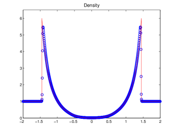
(b)

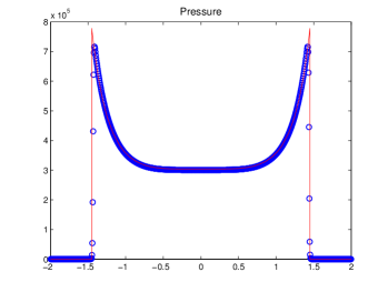
(c)

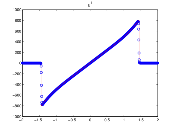
Figure 1: 1D Sedov blast wave problem. These panels show plots at time $t=0.001$ of (a) the density, (b) the pressure and (c) the velocity $u^{1}$. The solid lines are the exact solutions. The solution was obtained on a mesh with $\Delta x=1/200$ and a CFL of 0.35.

(a)

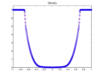
(b)

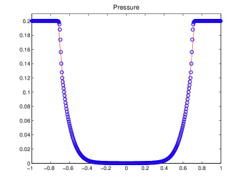
(c)

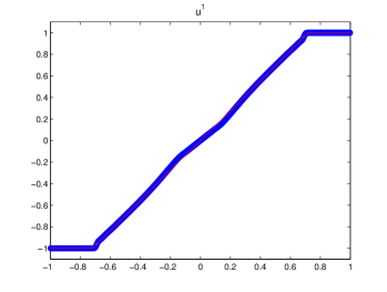
Figure 2: 1D double rarefaction problem. These panels show plots at time $t=0.6$ of (a) the density, (b) the pressure and (c) $u^{1}$. The solid lines are the exact solutions. The solution is obtained on a mesh with $\Delta x=1/200$ and a smaller CFL of $0.15$ that help to reduce unphysical oscillations.

(a)

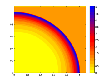
(b)

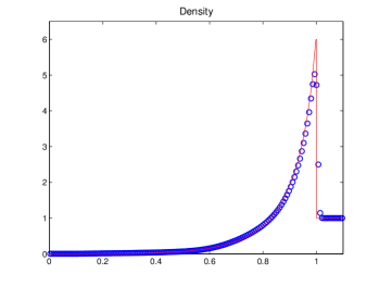
Figure 3: 2D Sedov blast wave problem. These panels show plots at time $t=1$ of (a) the density, and (b) a slice of the density along $y=0$. The solid line in (b) is the exact solution. The solution is obtained on a $160\times 160$ mesh and a CFL number of $0.35$.

(a)

(b)

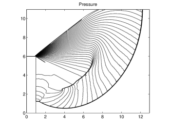
Figure 4: 2D Shock diffraction problem. These panels show plots at time $t=2.3$ of (a) the density, and (b) the pressure. A total of 20 equally spaced contour lines from $\rho=0.0662$ to $7.07$ are plotted in (a). We use 40 equally spaced contour lines from $p=0.091$ to $37$ are in (b). The solution is computed on a mesh with $\Delta x=\Delta y=1/30$ and a CFL number of $0.35$.

7 Conclusions and future work

In this paper we propose a high-order, single-stage, single-step, positivity-preserving method for the compressible Euler equations. The base scheme is the Taylor discretization of the Picard integral formulation of the PDE, where a single finite difference WENO reconstruction is applied once per time step. A positivity-preserving limiter is introduced in such a way that the positivity of the solution is preserved for the entire simulation, which adds a degree of robustness to our scheme. In addition, we have no excessive CFL restriction in order to retain positivity, which makes our new method more efficient compared to recent positivity-preserving methods. We demonstrate the effectiveness and efficiency of the positivity-preserving schemes on one- and two-dimensional problems with low density and pressure. High-order accuracy is retained after the introduction of our positivity preserving limiter on a test problem that has near zero pressure and density. Future work includes the construction of positivity-preserving multiderivative methods Seal2014 , applying the proposed method to other systems such as magnetohydrodynamics, as well as incorporating our method into an AMR framework.