Decaying dark matter: the case for a deep X-ray observation of Draco

Abstract

Recent studies of M31, the Galactic centre, and galaxy clusters have made tentative detections of an X-ray line at $\sim 3.5$ keV that could be produced by decaying dark matter. We use high resolution simulations of the Aquarius project to predict the likely amplitude of the X-ray decay flux observed in the GC relative to that observed in M31, and also of the GC relative to other parts of the Milky Way halo and to dwarf spheroidal galaxies. We show that the reported detections from M31 and the GC are compatible with each other, and with upper limits arising from high galactic latitude observations, and imply a decay time $\tau\sim 10^{28}$ seconds. We argue that this interpretation can be tested with deep observations of dwarf spheroidal galaxies: in 95 per cent of our mock observations, a 1.3 Msec pointed observation of Draco with XMM-Newton will enable us to discover or rule out at the 3$\sigma$ level an X-ray feature from dark matter decay at 3.5 keV, for decay times $\tau<0.8\times 10^{28}$ sec.

1 Introduction

One of the most pressing and interesting questions in fundamental physics and cosmology today is the identity of the dark matter (see e.g. Bertone 2010 and refs. therein). The properties of hypothetical dark matter particles remain largely unknown and there are many attempts to find phenomenological constraints on particular models from astronomical observations. For example, if dark matter particles were born relativistic, deep in the radiation-dominated epoch (so called “warm dark matter”, or WDM) they would affect the way structures were formed at small scales, leaving their imprints in the Lyman-$\alpha$ forest (e.g. Viel et al., 2005; Boyarsky et al., 2009a; Viel et al., 2013) and satellite galaxy abundances and structure (Polisensky & Ricotti, 2011; Kennedy et al., 2014; Lovell et al., 2014). Satellite structure may also provide limits on dark matter self-interactions (Vogelsberger et al., 2012; Zavala et al., 2013). One further constraint is the detection of electromagnetic radiation originating from the decay or annihilation of dark matter particles. Many studies to date have centred on attempts to detect the annihilation of weakly interacting massive particles (WIMPs) (see e.g. Bertone et al., 2005; Feng, 2010, for a review). This generic class of particles is attractive as a dark matter candidate due to their stability, their potential relation to electroweak symmetry breaking, and the possibility that they may be detected in laboratory experiments (see e.g. Cerdeño & Green, 2010, and refs. therein). WIMPs cannot decay, but are predicted to annihilate with one another in regions of high dark matter density, and could be detected via their annihilation products. Currently, the most interesting candidate WIMP signal is an excess of GeV photons from the centre of the Galaxy (Hooper & Goodenough, 2011; Daylan et al., 2014; Calore et al., 2014), but further evidence is needed to rule out a possible astrophysical origin of the signal (Boyarsky et al., 2011).

The interaction strength of weakly interacting massive particles limits their mass to the few GeV–few TeV range (in order to give the correct primordial abundance). Once the assumption about the interaction strength is relaxed, particle physics theories predict the existence of dark matter of different masses. If the particle mass is at the keV scale, and its lifetime longer than the age of the Universe, it may in principle be detectable indirectly, through the observation of X-ray photons produced by its decay (see e.g.  Dolgov & Hansen, 2002; Abazajian et al., 2001; Boyarsky et al., 2006; den Herder et al., 2009; Abazajian, 2009). An X-ray line signal consistent with such a decay has been identified at an energy of $\sim 3.5$ keV in galaxy clusters, in the Milky Way centre (or Galactic centre, GC) and in M31 by several studies (Boyarsky et al., 2014c, a; Bulbul et al., 2014a). although others have reported non-detections (Anderson et al., 2014; Malyshev et al., 2014) or reported detections but attributed them to have astrophysical origins (Jeltema & Profumo, 2014; Riemer-Sorensen, 2014 but see also Boyarsky et al., 2014b; Bulbul et al., 2014b). These two classes of systems – clusters and $L_{*}$ galaxies – are separated in mass by three orders of magnitude, therefore the correlation of the measured signal with expected projected dark matter mass is compelling evidence for dark matter decay as the origin of the signal.

These studies have based their estimates of the dark matter distribution in their targets on dark halo mass models that do not take into account fully the triaxiality of the halo, the presence of substructure, or the effects of baryons. Some of these issues have been examined in Bernal et al. (2014), who used a low resolution cosmological simulation containing $\sim 10^{5}$ Milky Way halo analogues to motivate better triaxial halo mass models. We instead make use of a series of high resolution simulations of Milky Way-analogue dark matter haloes, some of which were run with a full hydrodynamical treatment of the baryonic component, to estimate the X-ray decay signal from these targets and compare the results to the reported detections.

Targets such as the Milky Way and M31 are attractive due to their large projected mass densities, however their analysis is complicated by the presence of X-ray emission lines from the interstellar medium. Therefore, the nature of the line – dark matter or astrophysical – may be better ascertained by performing observations of objects with much cleaner backgrounds. One particularly promising class of candidates is that of the Milky Way’s dwarf spheroidal satellites (Boyarsky et al., 2006). These galaxies have very high mass-to-light ratios (Walker et al., 2009, 2010; Wolf et al., 2010), and very low gas fractions (Gallagher et al., 2003, and references therein). Their X-ray emitting gas fractions will be lower still due to their small gas fractions. Any detection from these galaxies would thus have a very low probability of an astrophysical origin and therefore dwarf spheroidal satellites have previously been targets of decaying DM searches in X-rays (Boyarsky et al., 2006, 2007; Loewenstein et al., 2009; Riemer-Sorensen & Hansen, 2009; Loewenstein & Kusenko, 2010; Mirabal, 2010; Loewenstein & Kusenko, 2012; Malyshev et al., 2014). With our set of simulations we can also set out to calculate the flux from dwarf spheroidals in their full cosmological context, including the contribution from the host halo.

In this work we use the high resolution simulations of the Aquarius project (Springel et al., 2008) to predict the likely amplitude of the X-ray decay flux observed in the GC relative to that observed in M31, and also of the GC relative to other parts of the Milky Way halo and to dwarf spheroidal galaxies. As we shall see, a sufficiently deep observation of the Draco dwarf galaxy would allow us to test the dark matter interpretation of the observed X-ray line signal in a very large region of the parameter space.

This paper is organised as follows. In Section 2 we present the simulations used in this paper. We discuss our methods for calculating the X-ray flux from the simulations in Section 3. In Section 4 we present our results for the expected fluxes of the GC, M31, and two dwarf spheroidal galaxies, and draw conclusions in Section 5. In the appendices we test the convergence of the simulations as function of resolution and number of sightlines (Appendix A), and consider the effects of cosmology, baryonic physics, and dark matter power spectrum (Appendix B). We present observational analysis and predictions for signal from Draco in Appendix C.

2 Simulations

Simulation	$m_{p}$ [$\mathrm{M_{\sun}}$]	$\epsilon$ [pc]	$M_{200}$ [$\mathrm{M_{\sun}}$]	$c$	$m_{\mathrm{WDM}}[\mathrm{keV}]$
Aq-A1	$1.712\times 10^{3}$	20.5	$1.839\times 10^{12}$	18.6	–
Aq-A2	$1.370\times 10^{4}$	65.8	$1.842\times 10^{12}$	18.5	–
Aq-A3	$4.911\times 10^{4}$	120.5	$1.836\times 10^{12}$	18.5	–
Aq-A4	$3.929\times 10^{5}$	342.5	$1.838\times 10^{12}$	18.6	–
Aq-A2(W7)	$1.545\times 10^{4}$	68.2	$1.938\times 10^{12}$	16.1	–
Aq-A2–$m_{1.5}$(W7)	$1.545\times 10^{4}$	68.2	$1.797\times 10^{12}$	15.9	1.456
Aq-A2–$m_{1.6}$(W7)	$1.545\times 10^{4}$	68.2	$1.802\times 10^{12}$	16.2	1.637
Aq-A2–$m_{2.0}$(W7)	$1.545\times 10^{4}$	68.2	$1.843\times 10^{12}$	16.0	2.001
Aq-A2–$m_{2.3}$(W7)	$1.545\times 10^{4}$	68.2	$1.875\times 10^{12}$	16.1	2.322
Aq-A4-S-NoWinds	$3.222\times 10^{5}$	342.5	$1.709\times 10^{12}$	25.1	–
Aq-A4-S-Winds	$3.222\times 10^{5}$	342.5	$1.590\times 10^{12}$	27.5	–
Aq-B2	$6.447\times 10^{3}$	65.8	$8.194\times 10^{11}$	11.7	–
Aq-C2	$1.399\times 10^{4}$	65.8	$1.774\times 10^{12}$	18.4	–
Aq-D2	$1.397\times 10^{4}$	65.8	$1.774\times 10^{12}$	12.4	–
Aq-E2	$9.593\times 10^{3}$	65.8	$1.185\times 10^{12}$	15.3	–

Table 1: Parameters of the simulations. We include the simulation dark matter particle mass $m_{p}$, the smoothing length $\epsilon$, the mass of the central halo encompassing a region of 200 times the critical density of the Universe, $M_{200}$, the halo concentration $c$, and the WDM particle mass, $m_{\mathrm{WDM}}$, where applicable. Concentration is determined by fitting NFW profiles to each halo at radii between 1 kpc and 100 kpc.

Each of the simulations used in this study is either taken directly from or derived from the Aquarius project. This is a set of Milky Way halo-analogue dark matter-only simulations run with the p-gadget3 code (Springel et al., 2008), and uses the cosmological parameters consistent with the one-year data of the Wilkinson Microwave Anisotropy Probe (WMAP1): $H_{0}=100h=73\mathrm{km/s/Mpc}$, $\Omega_{\mathrm{m}}=0.25$, $\Omega_{\Lambda}=0.75$, $\sigma_{8}=0.9$, and $n_{s}=1$ (Spergel et al., 2003). The six haloes are labelled Aq-A through to Aq-F. Aq-F was found to experience a major merger at redshift 0.4-0.5, and has been shown to be likely to host an S0 galaxy rather than a disc galaxy at redshift zero (Cooper et al., 2011): we therefore do not consider it in this study. The remaining five haloes span a range of masses and concentrations, and thus enable us to examine the effect of these parameters for different possible values of Milky Way and M31 mass and concentration.

The Aq-A halo has been rerun at five different simulation resolution levels for the purpose of checking that results are converged and not influenced by simulation resolution. These levels are labelled from 1 (highest resolution, particle mass $\sim 10^{3}\mathrm{M_{\sun}}$) to 5 (lowest resolution, particle mass $\sim 3\times 10^{6}\mathrm{M_{\sun}}$). The precise particle masses are reproduced in Table 1. Aq-A5 is very poorly resolved for the purposes of this experiment and is therefore not used here.

We determine the properties of DM structures using the subfind algorithm (Springel et al., 2001), which identifies bound overdensities as haloes and subhaloes. The largest subfind halo in each of the simulations is referred to as the ‘main halo’, and we take the Milky Way / M31 halo centre to be that of the main halo’s centre-of-potential. The positions of dwarf spheroidal candidates are likewise the centres-of-potential of dark matter subhaloes.

The original Aquarius runs are dark matter-only simulations, however it is likely that baryonic physics will have an impact on the distribution of dark matter in the Galaxy. We therefore make use of two gas physics resimulations of Aq-A4. Both have been run with the p-gadget3 code (Springel et al., 2008) and adopt the gas physics and star-formation prescriptions of Springel & Hernquist (2003). The two runs differ only in that one has the galactic winds model of Springel & Hernquist (2003) enabled whereas the other does not. The inclusion of winds inhibits further star-formation such that the stellar mass of the central galaxy is reduced from $1.45\times 10^{11}\mathrm{M_{\sun}}$ in the no-winds case to $9.19\times 10^{10}\mathrm{M_{\sun}}$ when winds are included. Both of these values are higher than the Milky Way stellar mass inferred by McMillan (2011, $6.43\pm 0.63\times 10^{10}\mathrm{M_{\sun}}$), so care should be taken when comparing these models to the Milky Way, especially the model that does not make use of the winds physics.

To check for the likely effect of our choice of cosmological parameters we have also performed a resimulation of Aq-A2 that instead uses the WMAP7 year values: $H_{0}=100h=70.4\mathrm{km/s/Mpc}$, $\Omega_{m}=0.272$, $\Omega_{\Lambda}=0.728$, $\sigma_{8}=0.81$, and $n_{s}=0.967$ (Komatsu et al., 2011). Since one candidate for producing the decay line is a 7.1keV sterile neutrino, which has the kinematic properties of WDM, we make use of four WDM simulations of Aq-A2 in the WMAP7 cosmology. These are identical to the Aq-A2-WMAP7 run except that the initial conditions wave amplitudes are rescaled with thermal relic WDM power spectra (Bode et al., 2001; Viel et al., 2005). The WDM models used have thermal relic particle masses 1.5keV, 1.6keV, 2.0keV, and 2.3keV. The 2.0keV model is a good approximation to a sterile neutrino produced in the presence of both very low and very high lepton asymmetries (Abazajian, 2014, Lovell et al. in prep.), and the other three enable us to examine the effect of larger and smaller effective particle masses. Further details about these simulations and the definition of WDM particle mass may be found in Lovell et al. (2014). Important properties for each of the simulations are given in Table 1.

3 Modelling the X-ray signal

We treat each simulation dark matter particle as a source of X-ray photons, which are emitted uniformly in all directions. It is simple to show that, for an inverse decay width $\tau$, the rate of photon production via this channel is:

$$\frac{dn}{dt}=\frac{N_{0}}{\tau}~{},$$ (1)

where $N_{0}$ is the (initial) number of dark matter particles that are represented by each simulation dark matter particle. We will adopt $\tau=10^{28}~{}\mathrm{s}$, which is close to the preferred value of Boyarsky et al. (2014c), for all of the results in this study except where indicated otherwise. In order to calculate the number of dark matter particles per simulation particle we set the particle mass to equal 7.1 keV, since this is the particle mass that would result in a two body decay for the 3.55 keV line. We also assume for our dark matter-only runs that baryons and dark matter have the same spatial distribution, and take the projected dark matter mass to be the universal dark matter mass fraction $\Omega_{\mathrm{DM}}/\Omega_{\mathrm{m}}$ multiplied by the total projected mass: we apply this fraction to all of our measurements that use dark matter-only simulations, including those for dwarf spheroidals.

We make use of two methods for calculating the flux from our chosen targets: sightlines for particular observer positions, and the spherically averaged flux for an observer at a given distance from the target. Both of these are discussed in detail below.

3.1 Sightlines

In this method we treat each simulation particle as a point source of X-ray photons. We randomly select positions on the surface of a sphere of some radius (8 kpc for the GC, 780 kpc for M31) around the centre of the largest subfind halo, and place our observers at these positions. We then define a cone with an opening angle of the XMM-Newton MOS field-of-view (FoV; $14^{\prime}$ radius) and central axis connecting the observer to the halo centre, and calculate the total flux of all simulation particles found within that cone: this is our ‘sightline’ measurement. For the measurements in which we observe the GC or M31 (‘on-centre’ measurements), the cone is directed towards the halo centre as described above; the procedures for ‘off-centre’ and dwarf spheroidal observations are described in Section 4.

All of our runs are zoom simulations, in which the halo of interest resides within a region of diameter $\sim 2$ Mpc populated with high resolution particles; the remainder of the box contains more massive, low resolution particles to provide the correct large scale forces. We use only the high resolution particles for our study. We find that our results are insensitive to any edge effects where the high resolution region ends, and we can truncate the region of particles sampled down to 50 kpc from the halo centre without affecting any of our results: we therefore do not impose any truncation. Background dark matter sources beyond the high resolution region will make a negligible contribution due to the redshifting of the emission, and are thus not included in the analysis (Boyarsky et al., 2006). In all cases we take the centre of the Milky Way (Sagittarius A*) to be at the simulated halo centre-of-potential as determined by our halo finder. We discuss briefly the number of sightlines required for our results to be robust in Section A.

3.2 Spherically averaged flux calculation

In this method we smear out each simulation particle into a spherical shell around the halo centre. We then calculate the flux from the shell surface area that intersects the line-of-sight cone as described above. This approach is equivalent to using an infinite number of sightlines. The numerical noise is reduced relative to the sightline method, with the penalty that we wash out anisotropies due to halo triaxiality and substructure.

It can be shown that the surface area of a spherical shell section contained within an observer FoV $\alpha$ situated a distance $d$ away from the shell centre is approximately:

$$A\approx 2\pi r(r\pm\alpha^{2}d-\sqrt{r^{2}-\alpha^{2}d^{2}})~{},$$ (2)

where $r$ is the sphere radius. The two solutions correspond to the surfaces intersected on either side of the shell: if the observer is located within the shell then only the solution with the plus sign is physical. We treat shells that fit entirely within the cone as point sources. The flux from the two portions is then:

$$F\approx\frac{N_{0}}{\tau}\frac{r\pm d\alpha^{2}-\sqrt{r^{2}-d^{2}\alpha^{2}}}{8\pi r(d\pm r)^{2}}~{},$$ (3)

and we can sum over all particles in the simulation to obtain the spherically-averaged flux of our target. This method is used in the appendix only, as a check for our sightline methods and to examine how the flux changes with distance to the halo centre.

4 Results

We now consider the effect of comparing different observations: on-centre vs. off-centre observations of the GC, on-centre GC vs. on-centre M31, and on-centre GC vs two dwarf spheroidal galaxies. All observers are placed at randomly selected positions around the centre of the target halo as described in subsection 3.1.

4.1 On-centre vs. off-centre observations

To begin, we generate 5000 ‘on-centre’ observations of the Aq-A1 halo as discussed in subsection 3.1, at a distance of 8kpc from the halo centre. In order to generate off-centre observations, we retain the positions used for the on-centre observers and target our sightlines in a random direction of some angular separation from the halo centre for 5000 sightlines; we do not attempt to identify or exclude sightlines that contain large substructures. We perform this procedure for a series of angular separations between 10 and 100 degrees in the Aq-A1 dataset. We take the ratio of each observer’s off-centre flux measurement and on-centre measurements and plot the results as a function of the offset angle, $\phi$, in Figure 1.

Figure 1: The ratio of off-centre flux to on-centre flux of the Aq-A1 halo as a function of angular separation from the halo centre. The crosses mark the median sightline flux for each distribution. The 95 per cent distributions are shown as solid lines and continued to 99 per cent as dashed lines. The dotted curve is fit to the median data and has the form $b^{n}[\phi+b]^{-n}$ where $b=4.3\,^{\circ}$ and $n=1.1$.

The flux ratios taper off with offset angle in a way that can be approximated by a power law. We impose a functional form of $b^{n}[\phi+b]^{-n}$ to the data, thus ensuring that the function has a value of 1 at 0 degrees. Our best fit for the median data is $b=4.3\,^{\circ}$ and $n=0.94$. We repeated the fitting procedure for the 95 per cent upper and lower bounds and found that the best fit parameters when using the same function were $b=4.5\,^{\circ},n=0.71$ and $b=4.1\,^{\circ},n=1.1$ respectively.

4.2 Blank sky observations

One particular application of off-centre measurements is the ability to obtain a blank sky dataset. Boyarsky et al. (2014c) used a stack of observations taken at several offset angles, for simplicity we use $100^{\circ}$. In the same way as for Figure 1 we calculate the ratio of the $100^{\circ}$ offset and on-centre measurements. We then bin up these ratios and plot the results in Figure 2 for Aq-A1, Aq-A2, and Aq-B2. We retrieve a broad distribution centred around 0.05 and obtain a very small probability density either below 0.02 or above 0.13. The 95 per cent lower bound of the ratio, as shown in the Figure, is 0.025. Boyarsky et al. (2014c) obtained a $2\sigma$ upper limit on the blank sky dataset flux of $0.7\times 10^{-6}\mathrm{cts/sec/cm}^{2}$; we would therefore expect the flux of the GC to be no higher than $\sim 3.6\times 10^{-5}\mathrm{cts/sec/cm}^{2}$ since it can be shown that the highest possible value of the GC flux would be the lowest value of this ratio multiplied by the $2\sigma$ error on the blank sky flux. The Aq-A2 curve differs somewhat from that of Aq-A1, which shows that we have not achieved good convergence at least for Aq-A2. We also include the result for Aq-B2, as this is the lightest halo and therefore perhaps the best GC candidate (albeit with a low concentration). When we combine the $2\sigma$ exclusion limit from Boyarsky et al. (2014c) with the reported detection in the GC ($2.9^{+0.5}_{-0.5}\times 10^{-5}\mathrm{cts/sec/cm}^{2}$; Boyarsky et al., 2014a) we obtain the shaded region shown in Figure 2. We also show the plot for observers in the plane of the inner halo minor axis, since this is the most likely orientation of the stellar disc with respect to the dark matter halo (Bailin et al., 2005; Aumer & White, 2013, see appendix subsection B.5). The distribution becomes skewed towards lower ratio values, however the lower limit to the distribution remains remarkably similar. There is some tension between the simulation result and the observational constraint. However, it should be noted that we do not attempt to identify sightlines that would be the most appropriate matches to blank sky targets such as the Lockman hole. Such sightlines may well have a lower projected mass density than that the unbiased selection offered here: actively selecting underdense light cones could well alleviate this tension.

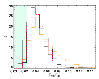
Figure 2: Histogram of the flux ratios for the $100^{\circ}$ Milky Way halo offset angle (black lines, Aq-A1 thick, Aq-A2 thin). We also plot the same result for Aq-B2 (orange), and again for Aq-A1 when observers are constrained to the plane normal to the minor axis vector (red dashed line). The vertical dotted line marks the 95 per cent lower bound on the flux distribution. The combined allowed region from the $2\sigma$ limit on the Boyarsky et al. (2014a) GC detection and the Boyarsky et al. (2014c) blank sky non-detection is given by the shaded green region.

4.3 M31 vs. GC observations

We now determine the likely ratio of the GC and M31 flux measurements. We assume initially that each of the five level 2 haloes used in our study (Aq-A to Aq-E) are all equally likely host haloes for the Milky Way and M31. We combine the lists of GC sightlines for each of the five haloes into one large catalogue, and likewise for the M31 sightlines. The simulations we use are resolution level 2; we multiply the flux of each GC sightline by a factor of 1.2 to compensate for resolution suppression as derived in Appendix A. We then extract one million randomly selected (with replacement, such that we can pick the same sightlines to be part of more than one pair) M31/GC sightline pairs in order to build a probability distribution function as the ratio of M31/GC observed flux. We plot the results for the combined list of sightlines in Figure 3.

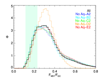
Figure 3: The probability distribution function for the M31/GC flux ratio. The result returned when all haloes are included is shown as the solid black line. The dotted lines correspond to cases where the data from one halo is omitted from the sample: Aq-A (blue), Aq-B (cyan), Aq-C (green), Aq-D (orange) and Aq-E(red). The shaded region corresponds to the $1\sigma$ uncertainty on the ratio of the detections of M31 Boyarsky et al. (2014c) and the GC Boyarsky et al. (2014a).

We find that the distribution peaks at $F_{\mathrm{M31}}/F_{\mathrm{GC}}=0.3$. The distribution as a whole is very broad: 95 per cent of the data is in the range [0.15,0.72]. To test how sensitive the result is to the properties of individual haloes, in the same Figure we also plot the same quantity whilst removing one halo at a time from the sample (as both a GC and M31 candidate). The position of the peak changes very little as a result of this procedure. However, the omission of the Aq-D halo from the sample is seen to remove much of the probability distribution at the high and low value tails: the 95 per cent bounds then tighten to [0.18,0.52]. The effect of removing any of the other four haloes is much smaller by comparison. The position of the peak varies between 0.23 and 0.33.

Boyarsky et al. (2014c, a) claim a detection from M31 of a line with flux $4.9^{+1.6}_{-1.3}\times 10^{-6}\mathrm{cts/sec/cm}^{2}$, and in the GC of $2.9^{+0.5}_{-0.5}\times 10^{-5}\mathrm{cts/sec/cm}^{2}$. Combining these two results and their associated errors, we obtain the shaded region shown in Figure 3. It is in broad agreement with all combinations of our haloes.

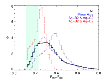
Figure 4: The probability distribution function for the M31/GC flux ratio is reproduced in black (all haloes). We also include data for observers in the plane of the minor axis (blue dotted line). The other two lines are obtained when our GC target is Aq-B2 and the M31 halo analogue is taken to be Aq-C2 (purple) and Aq-D2 (red). We reproduce the observational constraints as the shaded green region.

We now consider other variables that may affect the distribution of M31/GC flux ratios. In Figure 4 we plot three additional versions of the flux ratio histogram. The first is for GC observers constrained to reside in the inner-halo minor axis plane. The requirement that the observers reside in the minor axis plane has very little effect on the result. The second and third consider the case in which M31 is much more massive than the Milky Way (Peñarrubia et al., 2014). We take Aq-B2 – our smallest halo – to be our Milky Way candidate and Aq-C2 and Aq-D2 to be M31 halo candidates. Despite having the same mass to four significant figures, the flux histograms for the two combinations of GC and M31 (Aq-B2 – Aq-C2 vs. Aq-B2 – Aq-D2) are displaced by a factor of 1.6; the large difference in concentration (18.4 for Aq-C2, 12.4 for Aq-D2) plays an important role in the result.

4.4 Dwarf spheroidal galaxies

Additionally, one can hope to detect the signal in still more targets. Dwarf spheroidal galaxies are exceptionally good objects for further study (Boyarsky et al., 2006; Riemer-Sorensen & Hansen, 2009; Malyshev et al., 2014): they have very high mass-to-light ratios (e.g. Wolf et al., 2010), they represent a different mass regime to clusters and $L_{*}$ galaxies, and also contain very little if any interstellar gas (see Gallagher et al., 2003, and references therein). They therefore offer a set of circumstances in which the ratio of the predicted dark matter emission to the astrophysical background is very high.

The mass enclosed in the half-mass radius has been estimated by several studies (Walker et al., 2009, 2010; Wolf et al., 2010). Two of the satellites measured to have the highest central densities are Draco and Sculptor (Geringer-Sameth et al., 2014). We will select Draco and Sculptor candidates from our simulations and use these to make predictions for the likely amplitude of X-ray decay fluxes from these two satellites. We reproduce the observational data published in Wolf et al. (2010) in Table 2.

	Draco	Sculptor
$d$ (kpc)	$76\pm 5$	$86\pm 5$
$L$ ($L_{\odot,V}$)	$2.2^{+0.7}_{-0.6}\times 10^{5}$	$2.5^{+0.9}_{-0.7}\times 10^{6}$
$r_{1/2}$ (pc)	$291\pm 14$	$375\pm 54$
$M_{1/2}$ ($\mathrm{M_{\sun}}$)	$2.11^{+0.31}_{-0.31}\times 10^{7}$	$2.25^{+0.16}_{-0.15}\times 10^{7}$

Table 2: Selected parameters of the the Draco and Sculptor dwarf spheroidals as reproduced from Wolf et al. (2010): distance, $d$, luminosity, $L$, de-projected 3D half light radius, $r_{1/2}$, and half light mass, $M_{1/2}$.

We select Draco and Sculptor candidate subhaloes as follows. For each of our level 2 simulations we identify subhaloes that are between 88 and 148 kpc from the main halo centre. These values are chosen to increase our sample size beyond what is possible at the true distance of these satellites, such that the observer will be at a distance of 80-140kpc from the satellite. We then draw a sphere of radius equal to the Draco / Sculptor half-light radii around the subhalo centre. If the mass enclosed within that radius falls within the published uncertainty on the ‘half-light mass’ of the satellite galaxy in question then it is added to our sample. In this way we obtain 19 candidates for Draco and 33 for Sculptor. The shapes of the density profiles of these simulated subhaloes is quite different to that inferred for dwarf spheroidals by some studies (c.f. Springel et al., 2008; Walker & Peñarrubia, 2011 but see also Strigari et al., 2014) however our study is sensitive to the total subhalo mass within the satellite half-light radius alone, and not the density profile.

We place 5000 observers at random within the ring defined such that the observer-main halo distance is 8kpc and the observer-target subhalo distance is either 80, 90, 100, 110, 120, 130, or 140kpc from the centre as permitted by the main halo-subhalo separation. For subhalo positions such that more than one of these observer-target separations are possible we select the smallest available. We then calculate the flux from the target at the position of the observers in the same way as for the GC and M31. By this method we obtain the combined flux from the subhalo and the outskirts of the main halo. The results for both Draco and Sculptor are presented in Figure 5.

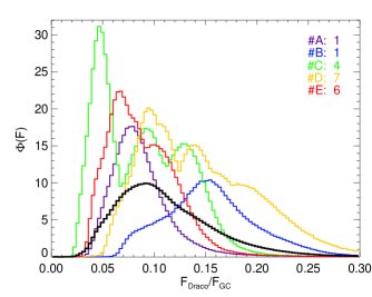
Figure 5: The probability distribution function envelopes for the flux ratios of Draco/GC (top panel) and Sculptor/GC (bottom panel). We calculate the normalised histogram for each individual satellite/GC pair and then, for each central halo, plot the curve that envelopes all of the curves associated with that central. The new histogram is not renormalised. The histograms for central haloes Aq-A2, Aq-B2, Aq-C2, Aq-D2, and Aq-E2 are shown in purple, blue, green, orange, and red respectively. The black line is the distribution obtained when all the distributions in each panel are merged.

There is a great deal of variation between different dwarf spheroidal candidates. For Draco the peak in the probability distribution may be as much as 20 per cent of the GC or as little as 5 per cent; for Sculptor the range in peaks is smaller. It it possible to see the effects of central halo concentration and mass: the Aq-D2 results are all clustered towards more modest ratios, as are those of Aq-B2.

4.5 Compatibility of X-ray line claims and limits in different targets

We now bring the results from each of these targets together to examine the likelihood that each (non-)detection is consistent with being generated by a dark matter particle of the same decay lifetime. In Figure 6 we plot the flux distributions for each of our targets as a function of projected mass for a series of different decay lifetimes $\tau_{27}=\tau/(10^{27}\mathrm{s})$. We take Aq-B2 to be our Milky Way candidate due to its low mass (Deason et al., 2012; Peñarrubia et al., 2014), and Aq-D2 to be our M31 analogue because of its relatively low concentration(Corbelli et al., 2010). We also include the $1\sigma$ allowed regions for the detections of the GC and M31, and also $2\sigma$ upper bounds for the blank sky dataset and Draco.

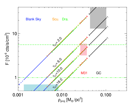
Figure 6: The distribution of fluxes from each of our targets as a function of the projected mass density for a series of four decay lifetimes ($\tau_{27}=2,6,10,18$). The GC (Aq-B2), M31 (Aq-D2), Draco (all candidates), Sculptor (all candidates) and Milky Way $100^{\circ}$ offset (Aq-B2) are denoted by the black, red, green, orange, and blue lines respectively. Lines are solid for the 95 per cent region and extended to 99 per cent with dashed lines. The grey shaded region denotes the $1\sigma$ allowed region from the GC detection of Boyarsky et al. (2014a), the red shaded region that of the M31 detection (Boyarsky et al., 2014c), and the blue shaded region the $2\sigma$ upper bound from the Boyarsky et al. (2014c) blank sky dataset. The dot-dashed green line represents the current $2\sigma$ upper bound on the flux from Draco (107.1 ks of XMM-MOS1 and XMM-MOS2 data; 40.4 ks XMM-PN data) and the triple-dot-dashed green line the $3\sigma$ limit that would be expected for $\sim 1.3$ Ms of XMM data. Good agreement between the simulation predictions and the observations is achieved when the lines overlap with their associated shaded regions for a single value of $\tau_{27}$.

We find that the best agreement between the corresponding simulation predictions and the observational constraints is approximately in the range $\tau_{27}=(6-10)$. This lifetime agrees within $1\sigma$ range with the results of Bulbul et al. (2014a); Boyarsky et al. (2014c, a) and is consistent with non-observation of the line from stacked observations of dSphs (Malyshev et al., 2014) where the limit $\tau_{27}>7.3$ ($3\sigma$ upper bound) was established. There is more tension with the limits from Anderson et al. (2014), who claim to rule out the line as found by (Bulbul et al., 2014a) at as much as $11.8\sigma$, however their applications of scaling relations and their stacking procedure may have consequences for the error estimates. These estimates are based on our haloes that are the best candidate matches for the Milky Way and GC. The projected mass will increase if the expected mass or concentration of either target were higher will cause the projected mass to change slightly. A proper implementation of baryon physics in particular will likely increases the projected mass densities (see Appendix B).

In addition to the published upper bound from the blank sky observations and also the published detections in the GC and M31, we include in Figure 6 the upper limit from the non-detection of Draco, as well as an estimate of the sensitivity of XMM-Newton with future observations. Based on archival data from the XMM-Newton observatory ($\sim 107$ks of MOS1+MOS2 instruments, and 40.4ks with PN) the $2\sigma$ upper bound is $5.6\times 10^{-6}\mathrm{cts/s/cm}^{2}$. Simulations using the Xspec’s (Arnaud, 1996) fakeit command find that a Draco flux of $\sim 1\times 10^{-6}\mathrm{cts/sec/cm}^{2}$ would be detected at $3\sigma$ with an XMM-Newton exposure of 1.34 Ms. For values of $\tau_{27}\sim 8$, 95 per cent of our realizations lead to an X-ray flux from Draco consistent with existing upper limits, and within the 3$\sigma$ reach of XMM-Newton with an exposure of 1.34 Ms.

5 Conclusions

The identity of the dark matter remains unknown. The detection of a series of unexplained lines in the X-ray spectra of a number of different astrophysical targets are suggested to be consistent with the decay of light dark matter particles. We have expanded on these studies by estimating the likely distribution of X-ray fluxes from these targets.

To this end we have used simulations of Milky Way-analogue dark matter haloes to ascertain the likely signal of the decay of dark matter into X-ray photons from the Galactic centre, M31 and two dwarf spheroidal galaxies. We placed 5000 observers at a distance of 8kpc around the simulated main halo centre and calculated the flux measured within the FoV of radius $14^{\prime}$, treating each simulation dark matter particle as a point source of X-ray photons. This procedure were also performed with observers 780kpc from the halo centre to simulate the likely M31 flux.

We then calculated the likely signal from other parts of the Milky Way halo. We performed an off-centre analysis in which we take a series of 5000 sightlines $100\,^{\circ}$ away from the main halo centre. We obtain a flux distribution that is slightly in tension with the 95 per cent exclusion limit from the Boyarsky et al. (2014c) blank sky dataset.

Pairs of GC and M31 measurements were compared to the ratio of fluxes found by Boyarsky et al. (2014c, a), and were found to be in good agreement for a wide range of sampling procedures.

Finally, we repeated the procedure for the Draco and Sculptor dwarf spheroidal satellite galaxies. We find a wide range of possible probability curves, with the central halo density as a very important parameter. Our results in this regime are consistent with a non-detection reported using $\sim 100$ks of archival XMM-Newton data, and future pointings of Draco will have the ability to rule out a dark matter decay signal from this object for values of $\tau_{27}<8$ at 95 per cent confidence.

Appendix A Resolution and Sightline Tests

We discuss here the convergence with numerical resolution of our simulations. In Figure 7 we plot surface density flux as a function of radius for a generic decaying dark matter particle of decay lifetime $\tau=10^{28}\mathrm{s}$, and are not interested in the mass of the dark matter particle. At the distance of M31, the separation between all four simulations is minimal and therefore we can consider even our level 4 simulation to resolve the system accurately. At smaller radii the curves start to diverge systematically with resolution. The flux amplitude at the GC distance is suppressed by 70 per cent in Aq-A4 relative to Aq-A1, compared to a difference in particle mass between the two runs of over two orders of magnitude. We also plot the expected flux for an Navarro-Frenk-White profile (NFW; Navarro et al., 1996, 1997) with the same $M_{200}$ and $c$ as our Aq-A1 halo ($M_{200}=1.839\times 10^{12}\mathrm{M_{\sun}}$ and $c=18.6$) for distances between 7 kpc and 500 kpc. It predicts approximately 22 per cent more flux than our Aq-A1 halo. However, Navarro et al. (2010) found that the Aquarius haloes were better described by an Einasto profile (Einasto, 1965) than by an NFW. The Einasto profile has a shallower central slope compared to the NFW, so the NFW curve may be interpreted as an upper limit on the ‘true’ flux. Therefore it is unlikely that a simulation of infinite resolution would return an GC flux more than $\sim 20$ per cent higher than that found in Aq-A1.

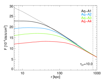
Figure 7: The expected X-ray flux from a Milky Way-analogue DM halo (Aq-A) as a function of distance from the halo centre. Each curve represents a different resolution simulation: Aq-A1 (black), Aq-A2 (blue), Aq-A3 (green), and Aq-A4 (red). The dotted line at 780 kpc marks the distance to M31, and the dashed line at 8 kpc the distance to the GC. We also include an NFW profile with the same $M_{200}$ and $c$ as the Aq-A1 halo (dotted line); it is normalised to the Aq-A1 curve at 50 kpc.

A more demanding criterion for convergence is that our sightline measurements converge. In Figure 8 we plot the distribution of fluxes for the GC and M31 for different resolution simulations of the Aq-A halo. The peak in the GC distribution moves to higher fluxes with increasing resolution, since the addition of more particles to the simulation increases the mass contained within the FoV on small scales. The distribution of the second highest resolution – Aq-A2 – is suppressed relative to that of the highest by 20 per cent, which is comparable to the suppression between these two simulations in Figure 7. Interestingly, the shape and width of the distribution changes very little between runs Aq-A2 and Aq-A1, which suggests that our derived bounds relative to the distribution peak for the fluxes will not be affected by resolution as much as the amplitude.

As was the case for the spherically-averaged method, the convergence of the M31 measurement is much better. The Aq-A1, Aq-A2, and Aq-A3 distributions all peak at the same flux and have very similar shapes. This is due to the physical radius of the FoV at the target in configuration space (740pc) being much larger than the spatial resolution of the simulation, unlike the GC case (only 8pc).

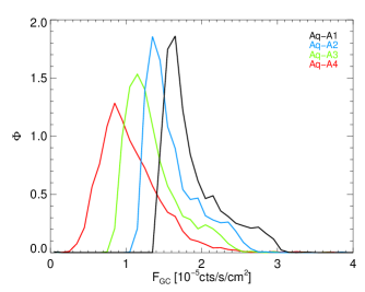
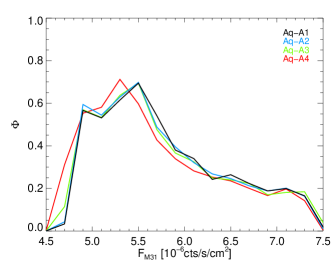
Figure 8: The flux distributions, $\Phi$, for the GC (left) and M31 (right) when different resolution simulations of the Aq-A halo are used as the target halo. Each distribution is normalised such that the area under the curve is equal to 1. The fluxes for Aq-A1, Aq-A2, Aq-A3, and Aq-A4 are shown in black, blue, green, and red respectively.

Finally, we checked that 5000 sightlines measurements are sufficient for the convergence of the flux distribution functions and adopt this number throughout.

Appendix B Influence of cosmology, baryon physics, and halo properties

In this section we examine the impact of various factors on our estimations of the fluxes from the GC and M31, including the possible effects of our choice of cosmological parameters, warm dark matter power spectra, baryons, and halo mass and concentration.

B.1 Cosmological parameters

First we consider the effect of cosmology. The halo properties will be sensitive to parameters such as the age of the Universe and at what redshift the halo centres form. In Figure 9 we plot the cumulative flux functions of the WMAP1 and WMAP7 versions of Aq-A2. In the GC and M31 regimes the WMAP7 flux distribution is suppressed relative to WMAP1 by up to 10 per cent. This occurs despite the increase in $M_{200}$ from WMAP1 to WMAP7; instead the halo becomes less concentrated. $\sigma_{8}$ has a lower value in WMAP7 compared to WMAP1 (see table 1), and this change delays the halo formation time to an epoch when the Universe is less dense (Lovell et al., 2014; Polisensky & Ricotti, 2014). Any such discrepancy may be magnified artificially by resolution issues since the WMAP7 run particle mass is slightly higher. In conclusion, it is likely that the choice of cosmological parameters will have a impact on the M31 and GC fluxes of not more than a few per cent.

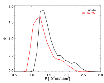
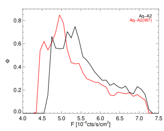
Figure 9: The flux distributions for Aq-A2 (black) and Aq-A2(W7) (red) for the GC (left) and M31 (right).

B.2 Warm dark matter

We now address the effect of changing the primordial matter power spectrum. One well-motivated candidate for decaying dark matter is a resonantly-produced sterile neutrino (Shi & Fuller, 1999; Laine & Shaposhnikov, 2008; Boyarsky et al., 2009b). A sterile neutrino with a mass of 7 keV has a non-negligible free-streaming length that erases small scale power in the early Universe. The resulting matter power spectrum therefore possesses a cutoff similar to that of warm dark matter (WDM). The position and slope of the cutoff is not uniquely determined by the sterile neutrino mass, as the sterile neutrino momentum distribution is modified in the presence of a lepton asymmetry, which is a relatively unconstrained parameter. The family of spectra for a sterile neutrino mass of 7 keV and an unconstrained lepton asymmetry has cutoffs in the range between those of a 2.0 keV and a 3.3 keV thermal WDM candidate (Abazajian, 2014, Lovell et al. in prep.). WDM models of this type have a considerable effect on the structure of dwarf galaxies (Lovell et al., 2012; Macciò et al., 2012, 2013; Shao et al., 2013; Schneider et al., 2014), and perhaps to a much smaller extent, on that of Milky Way-analogue haloes. In Figure 10 we plot the M31 sightlines measurement and the surface density flux as a function of radius for our WMAP7 version of Aq-A2 (CDM) and four WDM models (see figure caption).

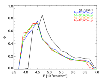
Figure 10: Impact of WDM. Left: The M31 flux distributions for Aq-A2(W7) as simulated with CDM (black) and WDM models of thermal relic particle masses 1.5kev (red), 1.6keV (orange), 2.0keV (green) and 2.3keV(blue). Right: The flux surface density as a function of radius for these five models.

The WDM flux distributions are suppressed relative to CDM for the M31 measurement by the order of a few per cent. The variation between WDM models is by comparison very small. The 1.5keV model is further suppressed than the 2.3keV, suggesting that flux correlates inversely with the free-streaming length, albeit weakly for this range of models. The discrepancy between CDM and the WDM models is reflected in the flux surface density profile, where CDM has a notably higher flux amplitude for observer distances greater than 40kpc. At the distance of M31 this again amounts to a few per cent. At the GC observer distance the separation is much smaller and no longer correlates consistently with dark matter free-streaming length. This result is reflected in the sightlines distribution for the GC (not shown). The 7keV sterile neutrinos will likely have a cooler power spectrum than that of even the 2.3keV thermal relic, therefore we do not consider further the effect of the dark matter free-streaming length on the flux distribution.

B.3 Baryonic physics

One crucial component of the cosmological model that is missing from the simulations presented so far is baryonic physics. Through the action of feedback and adiabatic contraction it is possible for baryons to alter considerably the distribution of dark matter and hence the expected X-ray flux (Blumenthal et al., 1986). We have run realisations of Aq-A4 (WMAP1) with two baryonic models. Both make use of the star-formation and gas physics prescriptions introduced in Springel & Hernquist (2003); one includes galactic winds and the other does not. With these simulations we are also able to relax the assumption that DM and baryons have the same spatial distribution. The M31 flux distribution functions for these simulations along with that of dark matter-only Aq-A4 are plotted in Figure 11.

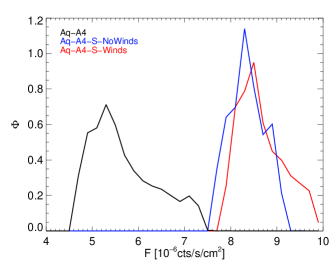
Figure 11: Impact of baryons. Left: The flux distributions from M31 for Aq-A4 as simulated with just dark matter (black), and two gas-hydro models: red includes winds and blue does not

.

The variation in flux distributions is substantial. Both baryon model simulations exhibit M31-distance flux distributions that are $\sim 50$ per cent higher than that of the DM-only run. Alternative gas/star-formation physics and subgrid recipes may produce different results (e.g. Schaller et al., 2014; Mollitor et al., 2015): here we simply state that the precise effect of gas physics is uncertain and likely to effect the outcome of our measurement for M31. Due to the poor resolution of the GC measurement in Aq-A4 we do not attempt to draw conclusions about the likely effect of baryons on the GC results. For the same reason, we also do not attempt to use the baryonic simulations for the dwarf spheroidals; the precise effect of baryonic physics on dwarf galaxy mass distribution has been highly debated in the literature (c.f. Di Cintio et al., 2012; Garrison-Kimmel et al., 2013; Brooks & Zolotov, 2014).

B.4 Halo sample variance

The measured flux will be very sensitive to the concentration of both the MW and M31 haloes, which decreases with halo mass albeit with considerable scatter (Gao et al., 2004; Neto et al., 2007). Also, individual haloes will have very stochastic formation histories, and so will likely have very different structures. We therefore use four further Aquarius haloes (B-E) to examine the scatter in flux measurements that is likely to result from these variations in halo properties. In Figure 12 we plot the GC and M31 flux distributions for Aq-A2 plus these extra four haloes, also simulated at resolution level 2.

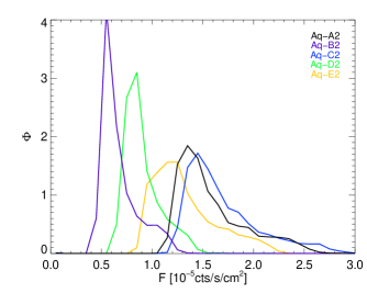
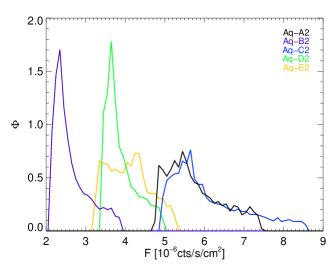
Figure 12: The flux distributions for Aq-A2 (black), Aq-B2 (purple), Aq-C2, (blue), Aq-D2 (green) and Aq-E2 (orange). The left panel is for the GC, the right for M31.

The GC flux distribution of the Aq-C2 halo is enhanced by over a factor of two relative to Aq-B2 (the least massive halo). It is also a factor of two larger than is the case for Aq-D2, which is remarkable in that the Aq-D2 and Aq-C2 haloes have the same mass to at least three significant figures. The underlying difference is halo concentration: the value of the concentration parameter $c$ is 18.4 for Aq-C2 and 12.4 for Aq-D2. The difference between haloes is even larger for the M31 case: therefore, the variation in halo concentration between our haloes will be very important for our results.

B.5 Position of observer

The final effect that we consider is that of the position of the observer within the Milky Way halo. It has been shown that the stellar disc is at its most stable when aligned with the inner dark matter halo’s minor axis (Bailin et al., 2005; Aumer & White, 2013), and that the orientation of these vectors is constant from the inner resolution limit to $0.1\times r_{200}$ (Vera-Ciro et al., 2011). We therefore calculate the inertia tensor of all the dark matter particles within the sphere of radius $0.1r_{200}$, extract the minor axis vector for the corresponding ellipsoid, and then randomly distribute observers in rings of radius 8kpc with the minor axis as the normal vector. We plot the distribution functions in Figure 13; for completeness we also include the results when the intermediate and major axes are used as the normal vector. The simulation used is Aq-A1.

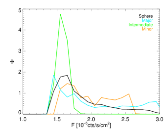
Figure 13: Flux distributions for the GC (Aq-A1) when the observer is constrained to lie in the plane normal to the minor (orange), intermediate (green) and major (cyan) axes; the spherically uniform sample is reproduced in black.

The different axes have a noticeable effect on the distribution of fluxes. The shapes of the constrained-observer curves have quite different shapes to the the spherical-sampling case. For the major axis measurement the distribution at low fluxes is remarkably similar to the spherical case, but is then skewed heavily towards higher fluxes. The minor axis has consistently higher fluxes than does spherical sampling, by up to a few tens of per cent. Given that the effect is non-negligible, we will therefore build the possiblity that our observer is biased towards the minor plane axis into our final results.

Appendix C Analysis of XMM-Newton/EPIC observations of Draco dwarf spheroidal galaxy

In this section we describe the details of our analysis of the Draco dwarf spheroidal galaxy (dSph) as observed with the European Photon Imaging Camera (EPIC) on-board the XMM-Newton space mission. Based on these observations, we fail to detect any significant line at $\sim 3.5$ keV, thus placing an upper bound on its strength. Finally, we estimated the exposure of Draco observations by XMM-Newton necessary to confirm the dark matter origin of the $\sim 3.5$ keV line. The results of this section have also been used for XMM-Newton proposal #076480, which was accepted in XMM-Newton 14th Announcement of Opportunity (AO-14); see http://xmm.esac.esa.int/external/xmm_news/otac_results/ao14_results for details.

C.1 Data reduction

In this paper we use data from the publicly available XMM-Newton observations of the Draco dSph (ObsIDs 0603190101, 0603190201, 0603190301, 0603190401 and 0603190501). Initial data files from the MOS and PN cameras of XMM-Newton/EPIC are pre-processed with the emproc and epproc procedures of the standard XMM-Newton software SAS v.13.5.0. We detect data patterns with significant spatial (bright point sources) and temporal (proton flares) variabilities using the standard SAS procedures espfilt and edetect_chain, remove these patterns from the subsequent analysis, and extract source spectra from 14’ radius circle centred on Draco dSph centre ($\mathrm{RA}={}$17:20:12.4, $\mathrm{DEC}=+$57:54:55.3) using SAS procedure evselect. Redistribution matrix files (RMF) and ancillary response files (ARF) are created with the standard SAS procedures rmfgen and arfgen, respectively. Finally, we group the obtained source spectra and response files, co-add them channel-by-channel using FTOOLS procedure addspec, and rebin the obtained spectra by 60 eV ($\sim 2-3$ times smaller than the instrument’s energy resolution) to make the energy bins roughly statistically independent. The total cleaned exposure of the obtained spectra is 107.1 ks for MOS (either MOS1 or MOS2) cameras and 40.4 ks for PN.

C.2 Spectral modelling

We model the obtained Draco spectra in the 0.8-10.0 keV range using the X-ray spectral fitting package Xspec v.12.8.1g. Because previous studies of dwarf spheroidal galaxies have not revealed the presence of any X-ray emitting gas, our model is a sum of instrumental and astrophysical background components. No signature of residual soft protons has been found according to the procedure of De Luca & Molendi (2004), so we have not added the residual soft proton component. The instrumental background (mostly caused by cosmic MeV protons penetrating inside XMM-Newton satellite) is modelled by an unfolded powerlaw model and the sum of several narrow gaussians representing bright fluorescence lines. The astrophysical background was modelled by a sum of the cosmic X-ray background (a folded powerlaw) and the Galactic X-ray background (two apec models), in full accordance with Malyshev et al. (2014). The resulting fit quality is good, with $\chi^{2}$ = 221.64 for 223 d.o.f. Then, by adding further narrow gaussian lines, we looked for line-like residuals in our region of interest near 3.5 keV. No statistically significant residuals were found. This produces a 2$\sigma$ upper bound of $5.6\times 10^{-6}$ cts/s/cm² on extra line flux in the 3.45-3.58 keV range.

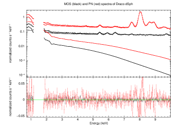
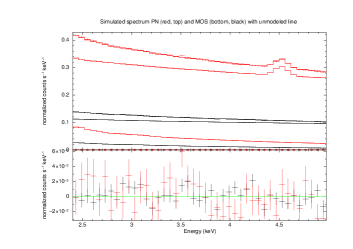
Figure 14: Left: Combined spectrum of existing Draco dSph observations modelled as a combination of folded components (absorbed thermal low energy Galactic emission), an extragalactic powerlaw (sharply falling component), and an instrumental component (unfolded powerlaw plus instrumental Gaussians). The quality of fit: $\chi^{2}=221.64$ per 223 d.o.f. Right: simulated spectrum of $1.34$ Ms of Draco dSph. The line with the flux $F_{\text{Draco,min}}$ is detected in two cameras with combined $\Delta\chi^{2}=13.0$.

C.3 Calculation of sensitivity with respect to narrow line at $\sim$3.5 keV

To determine the exposure of Draco observation necessary to check the decaying dark matter hypothesis of the $\sim$3.5 keV line, we first calculate the expected line strength. According to Figure 5, the best-fit ratio $F_{\text{Draco}}/F_{\text{GC}}=0.09$ with the scatter ranging from 0.04 to 0.2 (95 per cent range). Taking the results of Boyarsky et al. (2014a), where the line was detected from the GC with the highest significance, the best-fit line flux of $26\times 10^{-6}\,\mathrm{cts/s/cm^{2}}$ leads us to the conclusion that the range of fluxes expected from the Draco dSph is $(1.0-5.2)\times 10^{-6}\,\mathrm{cts/s/cm^{2}}$ with the most plausible value being $2.3\times 10^{-6}\,\mathrm{cts/s/cm^{2}}$. We take the value $F_{\text{Draco,min}}=1.0\times 10^{-6}\mathrm{cts/s/cm^{2}}$ as a conservative lower bound on the expected DM signal in Draco.

The existing observations of Draco (Fig. 14, left panel) allow us to determine the count rate at the energies of interest. It shows that one expects $N_{\text{bg}}=5.79\times 10^{4}$ cts (two MOS cameras combined) or $N_{\text{bg}}=8.36\times 10^{4}$ cts (PN camera) from a 1.34 Ms observation in a 180 eV energy interval (corresponding to the broadening of a narrow line due to the spectral resolution of XMM). Using the same exposure and the expected DM line flux of $1.02\times 10^{-6}\mathrm{cts/s/cm^{2}}$ we find $N_{\scriptscriptstyle\rm DM}=528$ cts for the MOS cameras (combined MOS1 and MOS2) and $N_{\scriptscriptstyle\rm DM}=600$ cts for the PN camera. Therefore the expected significance of the signal against this background is $N_{\scriptscriptstyle\rm DM}/\sqrt{N_{\text{bg}}}=(528+600)/\sqrt{(5.79+8.36)\times 10^{4}}\approx 3.0$.

To make this conclusion more robust we performed simulations of long-exposure observations. First, using the fakeit command of Xspec, we simulated realizations of the Draco dSph spectrum with the line added at the $10^{-6}\,\mathrm{cts/s/cm^{2}}$ level and with a XMM-Newton exposure 1.34 Ms: we recovered the line at a more than $3\sigma$ level. An example of the simulated spectrum with a positive line-like residual at $\sim 3.5$ keV is show in Fig. 14, right panel.

We also generate 250 realizations of spectra of a $1$ Ms observation of the Draco dSph (based on the model of the existing Draco data, see Fig. 14). The simulated spectra do not contain a line at $E\approx 3.5$ keV. We then try to detect a line at this energy and find that only in 12 simulations (i.e. in $4.8$ per cent of cases) were we able to detect a line-like residual at a level of $10^{-6}\,\mathrm{cts/s/cm^{2}}$ or above. This supports our estimate that a $1$ Ms observation will either confirm the existence of the line or will instead rule it out at least at the $95$ per cent confidence level.

In addition we have simulated 100 realizations of the Draco dSph spectrum with the line added at the $10^{-6}\,\mathrm{cts/s/cm^{2}}$ level. In 68 per cent of the realizations the line was recovered with a flux in the range $(0.71-1.45)\times 10^{-6}\,\mathrm{cts/s/cm^{2}}$, consistent with the Gaussian scatter around the simulated value.

References

- Abazajian et al. (2001) Abazajian K., Fuller G. M., Tucker W. H., 2001, Astrophys.J., 562, 593
- Abazajian (2009) Abazajian K. N., 2009, white paper submitted to the Astro 2010 Decadal Survey, Cosmology and Fundamental Physics Science
- Abazajian (2014) Abazajian K. N., 2014, Physical Review Letters, 112, 161303
- Abazajian et al. (2007) Abazajian K. N., Markevitch M., Koushiappas S. M., Hickox R. C., 2007, Phys.Rev., D75, 063511
- Anderson et al. (2014) Anderson M. E., Churazov E., Bregman J. N., 2014, ArXiv e-prints
- Arnaud (1996) Arnaud K. A., 1996, in A.S.P. Conference Serie, Vol. 101, Astronomical Data Analysis Software and Systems V, Jacoby G. H., Barnes J., eds., San Francisco, ASP, p. 17
- Aumer & White (2013) Aumer M., White S. D. M., 2013, MNRAS, 428, 1055
- Bailin et al. (2005) Bailin J. et al., 2005, ApJ, 627, L17
- Bernal et al. (2014) Bernal N., Forero-Romero J. E., Garani R., Palomares-Ruiz S., 2014, JCAP, 9, 4
- Bertone et al. (2005) Bertone G., Hooper D., Silk J., 2005, Phys.Rept., 405, 279
- Bertone (2010) Bertone G. e., 2010
- Blumenthal et al. (1986) Blumenthal G. R., Faber S. M., Flores R., Primack J. R., 1986, ApJ, 301, 27
- Bode et al. (2001) Bode P., Ostriker J. P., Turok N., 2001, ApJ, 556, 93
- Boyarsky et al. (2014a) Boyarsky A., Franse J., Iakubovskyi D., Ruchayskiy O., 2014a, ArXiv e-prints
- Boyarsky et al. (2014b) Boyarsky A., Franse J., Iakubovskyi D., Ruchayskiy O., 2014b, ArXiv e-prints
- Boyarsky et al. (2008) Boyarsky A., Iakubovskyi D., Ruchayskiy O., Savchenko V., 2008, Mon.Not.Roy.Astron.Soc., 387, 1361
- Boyarsky et al. (2009a) Boyarsky A., Lesgourgues J., Ruchayskiy O., Viel M., 2009a, JCAP, 5, 12
- Boyarsky et al. (2011) Boyarsky A., Malyshev D., Ruchayskiy O., 2011, Physics Letters B, 705, 165
- Boyarsky et al. (2006) Boyarsky A., Neronov A., Ruchayskiy O., Shaposhnikov M., Tkachev I., 2006, Physical Review Letters, 97, 261302
- Boyarsky et al. (2006) Boyarsky A., Neronov A., Ruchayskiy O., Shaposhnikov M., Tkachev I., 2006, Phys.Rev.Lett., 97, 261302
- Boyarsky et al. (2007) Boyarsky A., Nevalainen J., Ruchayskiy O., 2007, Astron.Astrophys., 471, 51
- Boyarsky et al. (2014c) Boyarsky A., Ruchayskiy O., Iakubovskyi D., Franse J., 2014c, Physical Review Letters, 113, 251301
- Boyarsky et al. (2010) Boyarsky A., Ruchayskiy O., Iakubovskyi D., Walker M. G., Riemer-Sorensen S., et al., 2010, Mon.Not.Roy.Astron.Soc., 407, 1188
- Boyarsky et al. (2009b) Boyarsky A., Ruchayskiy O., Shaposhnikov M., 2009b, Annual Review of Nuclear and Particle Science, 59, 191
- Brooks & Zolotov (2014) Brooks A. M., Zolotov A., 2014, ApJ, 786, 87
- Bulbul et al. (2014a) Bulbul E., Markevitch M., Foster A., Smith R. K., Loewenstein M., Randall S. W., 2014a, ApJ, 789, 13
- Bulbul et al. (2014b) Bulbul E., Markevitch M., Foster A. R., Smith R. K., Loewenstein M., Randall S. W., 2014b, ArXiv e-prints
- Calore et al. (2014) Calore F., Cholis I., Weniger C., 2014
- Cerdeño & Green (2010) Cerdeño D. G., Green A. M., 2010, Direct detection of WIMPs, Bertone G., ed., Cambridge University Press, p. 347
- Cooper et al. (2011) Cooper A. P. et al., 2011, ApJ, 743, L21
- Corbelli et al. (2010) Corbelli E., Lorenzoni S., Walterbos R., Braun R., Thilker D., 2010, A&A, 511, A89
- Daylan et al. (2014) Daylan T., Finkbeiner D. P., Hooper D., Linden T., Portillo S. K. N., et al., 2014
- De Luca & Molendi (2004) De Luca A., Molendi S., 2004, A&A, 419, 837
- Deason et al. (2012) Deason A. J., Belokurov V., Evans N. W., An J., 2012, MNRAS, L469
- den Herder et al. (2009) den Herder J., Boyarsky A., Ruchayskiy O., Abazajian K., Frenk C., et al., 2009, a white paper submitted in response to the Fundamental Physics Roadmap Advisory Team (FPR-AT) Call for White Papers
- Di Cintio et al. (2012) Di Cintio A., Knebe A., Libeskind N. I., Brook C., Yepes G., Gottloeber S., Hoffman Y., 2012, ArXiv e-prints
- Dolgov & Hansen (2002) Dolgov A., Hansen S., 2002, Astropart.Phys., 16, 339
- Einasto (1965) Einasto J., 1965, Trudy Astrofizicheskogo Instituta Alma-Ata, 5, 87
- Feng (2010) Feng J. L., 2010, Ann.Rev.Astron.Astrophys., 48, 495
- Gallagher et al. (2003) Gallagher J. S., Madsen G. J., Reynolds R. J., Grebel E. K., Smecker-Hane T. A., 2003, ApJ, 588, 326
- Gao et al. (2004) Gao L., White S. D. M., Jenkins A., Stoehr F., Springel V., 2004, MNRAS, 355, 819
- Garrison-Kimmel et al. (2013) Garrison-Kimmel S., Rocha M., Boylan-Kolchin M., Bullock J. S., Lally J., 2013, MNRAS, 433, 3539
- Geringer-Sameth et al. (2014) Geringer-Sameth A., Koushiappas S. M., Walker M., 2014, ArXiv e-prints
- Hooper & Goodenough (2011) Hooper D., Goodenough L., 2011, Physics Letters B, 697, 412
- Horiuchi et al. (2014) Horiuchi S., Humphrey P. J., Onorbe J., Abazajian K. N., Kaplinghat M., et al., 2014, Phys.Rev., D89, 025017
- Jeltema & Profumo (2014) Jeltema T. E., Profumo S., 2014, ArXiv e-prints
- Kennedy et al. (2014) Kennedy R., Frenk C., Cole S., Benson A., 2014, MNRAS, 442, 2487
- Komatsu et al. (2011) Komatsu E. et al., 2011, ApJS, 192, 18
- Laine & Shaposhnikov (2008) Laine M., Shaposhnikov M., 2008, JCAP, 6, 31
- Loewenstein & Kusenko (2010) Loewenstein M., Kusenko A., 2010, Astrophys.J., 714, 652
- Loewenstein & Kusenko (2012) Loewenstein M., Kusenko A., 2012, Astrophys.J., 751, 82
- Loewenstein et al. (2009) Loewenstein M., Kusenko A., Biermann P. L., 2009, Astrophys.J., 700, 426
- Lovell et al. (2012) Lovell M. R. et al., 2012, MNRAS, 420, 2318
- Lovell et al. (2014) Lovell M. R., Frenk C. S., Eke V. R., Jenkins A., Gao L., Theuns T., 2014, MNRAS, 439, 300
- Macciò et al. (2012) Macciò A. V., Paduroiu S., Anderhalden D., Schneider A., Moore B., 2012, MNRAS, 3204
- Macciò et al. (2013) Macciò A. V., Paduroiu S., Anderhalden D., Schneider A., Moore B., 2013, MNRAS, 428, 3715
- Malyshev et al. (2014) Malyshev D., Neronov A., Eckert D., 2014, Phys. Rev. D, 90, 103506
- McMillan (2011) McMillan P. J., 2011, MNRAS, 414, 2446
- Mirabal (2010) Mirabal N., 2010, MNRAS, 409, L128
- Mollitor et al. (2015) Mollitor P., Nezri E., Teyssier R., 2015, MNRAS, 447, 1353
- Navarro et al. (1996) Navarro J. F., Frenk C. S., White S. D. M., 1996, ApJ, 462, 563
- Navarro et al. (1997) Navarro J. F., Frenk C. S., White S. D. M., 1997, ApJ, 490, 493
- Navarro et al. (2010) Navarro J. F. et al., 2010, MNRAS, 402, 21
- Neto et al. (2007) Neto A. F. et al., 2007, MNRAS, 381, 1450
- Peñarrubia et al. (2014) Peñarrubia J., Ma Y.-Z., Walker M. G., McConnachie A., 2014, MNRAS, 443, 2204
- Polisensky & Ricotti (2011) Polisensky E., Ricotti M., 2011, Phys. Rev. D, 83, 043506
- Polisensky & Ricotti (2014) Polisensky E., Ricotti M., 2014, MNRAS, 437, 2922
- Riemer-Sorensen (2014) Riemer-Sorensen S., 2014, ArXiv e-prints
- Riemer-Sorensen & Hansen (2009) Riemer-Sorensen S., Hansen S. H., 2009, A&A, 500, L37
- Riemer-Sorensen et al. (2006) Riemer-Sorensen S., Hansen S. H., Pedersen K., 2006, Astrophys.J., 644, L33
- Schaller et al. (2014) Schaller M. et al., 2014, ArXiv e-prints
- Schneider et al. (2014) Schneider A., Anderhalden D., Macciò A. V., Diemand J., 2014, MNRAS, 441, L6
- Shao et al. (2013) Shao S., Gao L., Theuns T., Frenk C. S., 2013, MNRAS, 430, 2346
- Shi & Fuller (1999) Shi X., Fuller G. M., 1999, Physical Review Letters, 82, 2832
- Spergel et al. (2003) Spergel D. N. et al., 2003, ApJS, 148, 175
- Springel & Hernquist (2003) Springel V., Hernquist L., 2003, MNRAS, 339, 312
- Springel et al. (2008) Springel V. et al., 2008, MNRAS, 391, 1685
- Springel et al. (2001) Springel V., White S. D. M., Tormen G., Kauffmann G., 2001, MNRAS, 328, 726
- Strigari et al. (2014) Strigari L. E., Frenk C. S., White S. D. M., 2014, ArXiv e-prints
- Vera-Ciro et al. (2011) Vera-Ciro C. A., Sales L. V., Helmi A., Frenk C. S., Navarro J. F., Springel V., Vogelsberger M., White S. D. M., 2011, MNRAS, 416, 1377
- Viel et al. (2013) Viel M., Becker G. D., Bolton J. S., Haehnelt M. G., 2013, Phys. Rev. D, 88, 043502
- Viel et al. (2005) Viel M., Lesgourgues J., Haehnelt M. G., Matarrese S., Riotto A., 2005, Phys. Rev. D, 71, 063534
- Vogelsberger et al. (2012) Vogelsberger M., Zavala J., Loeb A., 2012, MNRAS, 3127
- Walker et al. (2009) Walker M. G., Mateo M., Olszewski E. W., Peñarrubia J., Wyn Evans N., Gilmore G., 2009, ApJ, 704, 1274
- Walker et al. (2010) Walker M. G., Mateo M., Olszewski E. W., Peñarrubia J., Wyn Evans N., Gilmore G., 2010, ApJ, 710, 886
- Walker & Peñarrubia (2011) Walker M. G., Peñarrubia J., 2011, ApJ, 742, 20
- Watson et al. (2006) Watson C. R., Beacom J. F., Yuksel H., Walker T. P., 2006, Phys.Rev., D74, 033009
- Watson et al. (2012) Watson C. R., Li Z., Polley N. K., 2012, JCAP, 3, 18
- Wolf et al. (2010) Wolf J., Martinez G. D., Bullock J. S., Kaplinghat M., Geha M., Muñoz R. R., Simon J. D., Avedo F. F., 2010, MNRAS, 406, 1220
- Zavala et al. (2013) Zavala J., Vogelsberger M., Walker M. G., 2013, MNRAS, 431, L20